Sample variance in photometric redshift calibration: cosmological biases and survey requirements
Abstract
We use N-body/photometric galaxy simulations to examine the impact of sample variance of spectroscopic redshift samples on the accuracy of photometric redshift (photo-z) determination and calibration of photo-z errors. We estimate the biases in the cosmological parameter constraints from weak lensing and derive requirements on the spectroscopic follow-up for three different photo-z algorithms chosen to broadly span the range of algorithms available. We find that sample variance is much more relevant for the photo-z error calibration than for photo-z training, implying that follow-up requirements are similar for different algorithms. We demonstrate that the spectroscopic sample can be used for training of photo-zs and error calibration without incurring additional bias in the cosmological parameters. We provide a guide for observing proposals for the spectroscopic follow-up to ensure that redshift calibration biases do not dominate the cosmological parameter error budget. For example, assuming optimistically (pessimistically) that the weak lensing shear measurements from the Dark Energy Survey could obtain constraints on the dark energy equation of state of 0.035 (0.055), implies a follow-up requirement of 150 (40) patches of sky with a telescope such as Magellan, assuming a effective field of view and 400 galaxies per patch. Assuming (optimistically) a VVDS-like spectroscopic completeness with purely random failures, this could be accomplished with about 75 (20) nights of observation. For more realistic assumptions regarding spectroscopic completeness, or with the presence of other sources of systematics not considered here, further degradations to dark energy constraints are possible. We test several approaches for making the requirements less stringent. For example, if the redshift distribution of the overall sample can be estimated by some other technique, e.g. cross-correlation, then follow-up requirements could be reduced by an order of magnitude.
1 Introduction
One of the principal systematic errors affecting surveys that utilize the large-scale structure to study dark energy is the quality of the photometric redshifts (hereafter photo-zs). Due to time and throughput constraints it is costly and impractical to obtain spectroscopic redshifts for more than a small fraction of galaxies. Upcoming surveys such as the Dark Energy Survey11 1 http://darkenergysurvey.org (DES), PanStarrs22 2 http://pan-starrs.ifa.hawaii.edu, Hyper-Suprime Cam survey33 3 http://oir.asiaa.sinica.edu.tw/hsc.php (HSC) and the Large Synoptic Survey Telescope44 4 http://lsst.org (LSST) will have to rely on the photo-zs in order to utilize the three-dimensional information from the large number of galaxies observed in these surveys. Without the redshift information, one loses the ability to perform weak lensing tomography Hu (1999), and thus degrades the ability to measure the temporal evolution of dark energy in the recent () history of the universe (Bartelmann & Schneider, 2001; Huterer, 2002; Hu, 2002; Munshi et al., 2008; Hoekstra & Jain, 2008; Amara & Refregier, 2007; Huterer, 2010, for reviews, see).
Photo-z techniques use broad-band photometry, i.e. the measured flux through a few bands, to estimate approximate galaxy redshifts. Other observable quantities (hereafter ’observables’), such as galaxy shape measures, can also be used, but they typically have limited redshift information. The intrinsic uncertainty of photo-zs can contribute significantly to the error in the inferred cosmological parameters.
There are two broad, overlapping, categories of photo-z estimators. Template-fitting algorithms (Arnouts et al., 1999; Bolzonella et al., 2000; Benitez, 2000; Budavári et al., 2000; Csabai et al., 2003; Feldmann et al., 2006, e.g.) assign photo-zs to a galaxy by finding the template and redshift that best reproduce the observed fluxes. Training set methods (Connolly et al., 1995; Firth et al., 2003; Wadadekar, 2005; Wang et al., 2007; Gerdes et al., 2010, e.g.), on the other hand, use a spectroscopic sample to characterize a relation between the photometric observables and the redshifts, which is then applied to the full photometric sample. The distinction between the two categories is muddled because template-fitting methods can also use spectroscopic redshifts to improve the fitting. Conversely, training set methods can be based on catalogs simulated using templates. For reviews and comparison of methods see, e.g. Hogg et al. (1998); Koo (1999); Hildebrandt et al. (2010); Abdalla et al. (2011).
Spectroscopic redshifts (hereafter spec-zs) play three important roles in photo-z analysis. First, as described above they improve the accuracy of photo-z estimation. Having accurate photo-zs is highly desirable for cosmology, as photo-z errors inevitably smear the radial information describing galaxy clustering. Second, spectroscopic redshifts characterize the photo-z errors (see Ref. Oyaizu et al., 2008a, for a review). With accurate error estimation, one can remove or downweight the less reliable photo-zs, decreasing their impact on the cosmological analysis. Third, spec-zs characterize the uncertainties in the photo-z error distribution (’error in the error’), which is a key quantity that needs to be accurately known. In particular, even if photo-zs are not exceptionally accurate and there are regions of badly misestimated redshift (i.e. the ’catastrophic errors’), one can still recover the cosmological information provided the bias, scatter, and ideally the full distribution in the plane, are accurately calibrated using the subset of galaxies with spectroscopic information.
The requirements on spectroscopic samples due to the three requirements mentioned are not independent, but have been treated as such in the past. For example, the amount of spectroscopic follow-up required for calibration depends on the intrinsic accuracy of the photo-zs (Ma et al., 2006; Huterer et al., 2006; Ma & Bernstein, 2008) and on the identification of regions with unreliable photo-zs (Bernstein & Huterer, 2010; Sun et al., 2009; Hearin et al., 2010), but the ability to do both of these is strongly dependent on the use of spec-zs for training and error estimation. At this point, the careful reader may wonder: can the same spectroscopic sample be used for photo-z training, error estimation and calibration without significantly biasing cosmological results? Yes, it turns out, as we will show in this paper.
Obtaining spectra for thousands of galaxies needed for photo-z studies is a very difficult task, which complicates their use in photo-z studies. Spectroscopic surveys can be far from a representative sub-sample of the photometric sample for five principal reasons:
- •
Shot noise: Spectroscopic samples to the depth required are quite small, hence Poisson fluctuations due to the finite number of galaxies are significant.
- •
Sample variance: Spectroscopic surveys designed to reach the magnitude limits of the upcoming photometric surveys typically have very small angular apertures, much smaller than fluctuations introduced by large-scale clustering of galaxies. The fluctuations due to sample variance can be an order of magnitude larger than shot-noise fluctuations for samples of around (see e.g. van Waerbeke et al., 2006, and Fig. 1).
- •
Type incompleteness: Strength of spectral features vary significantly with galaxy type. In addition, the wavelength coverage of most spectrographs is not sufficient to detect some of the main features through the full redshift range of interest.
- •
Incorrect redshifts: Line misidentification can yield incorrect redshifts. The number of incorrect spectroscopic redshifts can be reduced – by keeping only the most reliable galaxies – at the cost of increasing the incompleteness.
- •
Sample variance in observing conditions: Variations in imaging conditions (e.g. seeing and photometric quality) during a survey imprint an angular dependence to the survey depth and completeness.
Past papers on the effects of photometric redshift errors on dark energy constraints (Ma et al., 2006; Huterer et al., 2006; Amara & Refregier, 2007; Abdalla et al., 2008; Ma & Bernstein, 2008; Kitching et al., 2008; Bordoloi et al., 2010; Hearin et al., 2010) have studied in detail the distribution of photometric redshifts (more specifically, the full probability density function ). Some of these works have extended the analysis to estimate the number of spectra required in order to calibrate the photo-zs. However, in essentially all cases the requirements on the spectroscopic sample have only assumed shot noise, i.e. that the accuracy of the photo-z bias and error in some redshift bin labeled by is equal to and , where is the size of the spectroscopic follow-up sample in that bin (Ma et al., 2006, see Eq. (18) in Ref.).
Sample variance was taken into account in spectroscopic follow-up requirements in van Waerbeke et al. (2006); Ishak & Hirata (2005); however, they only considered the overall redshift distribution of the source sample and did not include photometric redshifts in the simulations (see also Bordoloi et al., 2010, for a related discussion). Requirements on spectrograph design in order to minimize spectroscopic failures were investigated in Jouvel et al. (2009), with emphasis on designing spectrographs to calibrate redshifts for space-based missions. Finally, the effects of sample variance in observing conditions was investigated by Nakajima et al. (2012) using SDSS imaging and spectroscopic redshifts from several surveys overlapping the SDSS. That paper found that atypical imaging conditions in the spectroscopic fields can lead to biases in galaxy-galaxy lensing analysis, but fortunately concluded that this type of bias can be at least partly corrected (see also Sheldon et al., 2011, for a related discussion).
The main goals of this paper are to study the impact of sample variance in spectroscopic samples to the training of photo-zs, error estimation and error calibration, and to assess implications for cosmological constraints from weak lensing tomography analyses. The paper is organized as follows. In Sec. 2 we describe the photo-z algorithms we use in our tests. In Sec. 3 we describe our construction of the different simulated samples used. We detail the procedure of estimating biases in cosmological constraints from the weak lensing tomography in Sec. 4. Results are given in Sec. 5 with a discussion of potential improvements in Sec. 6. We provide a guide for determining spectroscopic observational requirements in Sec. 7 and present our conclusions in Sec. 8. The construction of the simulations is described in Appendix A.
2 Photo-z algorithms
We consider three different photo-z algorithms that broadly span the space of possibilities. Namely, we use a basic template-fitting code without any priors, a training set fitting method, and a training set method that does not perform a fit, but uses the local density in the neighborhood of an object to derive a redshift probability distribution. We briefly describe each below.
2.1 Template-fitting redshift estimators
Template-fitting estimators derive photometric redshift estimates by comparing the observed colors of galaxies to colors predicted from a library of galaxy spectral energy distributions. We use the publicly available LePhare photo-z code55 5 http://www.cfht.hawaii.edu/~arnouts/LEPHARE/lephare.html (Arnouts et al., 1999; Ilbert et al., 2006) as our template-fitting estimator. We chose the extended CWW template library (Coleman et al., 1980) because it yielded the best photo-z’s for our simulation.
We purposefully ignore all priors for reasons that we now describe. There are essentially two classes of priors, those derived from completely different surveys, and those based on targeted follow-ups of a subsample of the survey for which photo-z’s are desired. The use of the latter makes template-fitting results quite similar to the training set methods, and would make the template-fitting code subject to a training procedure which would be affected by the sample variance. The use of the former could reduce some outliers, but would also complicate the interpretation of the results; there are several choices of external priors, and if the selection of the sample used to determine the priors is different from that of the survey at hand then redshifts could be biased (Abrahamse et al., 2011, see, e.g.). As we shall see, the photo-z quality is not a dominant factor in our analysis, and a more thorough experimentation of the template-fitting algorithms is not expected to affect conclusions.
2.2 Nearest-neighbor redshift probability estimators
2.2.1 Weights
In this subsection, we briefly review the weighting method66 6 The weights, and polynomial codes are available at http://kobayashi.physics.lsa.umich.edu/~ccunha/nearest/. The codes can also be obtained in the git repository probwts at http://github.com of Lima et al. (2008), which is required for computing redshift probabilities, henceforth . We define the weight, , of a galaxy in the spectroscopic training set as the normalized ratio of the density of galaxies in the photometric sample to the density of training-set galaxies around the given galaxy. These densities are calculated in a local neighborhood in the space of photometric observables, e.g. multi-band magnitudes. In this case, the DES griz magnitudes are our observables. The hypervolume used to estimate the density is set here to be the Euclidean distance of the galaxy to its nearest-neighbor in the training set. We set for the estimate. Smaller lead to less broad s and better reconstruction of the overall redshift distribution at the cost of increased shot-noise in individual s. If one does not care about individual s then we recommend choosing a smaller N; the optimal choice will depend on the training set size. The bias analysis is not sensitive to the choice of .
The weights can be used to estimate the redshift distribution of the photometric sample using
| (1) |
where the weighted sum is over all galaxies in the training set. Lima et al. (2008) and Cunha et al. (2009) show that this provides a nearly unbiased estimate of the redshift distribution of the photometric sample, , provided the differences in the selection of the training and photometric samples are solely done in the observable quantities used to calculate the weights.
2.2.2 Probability density
To estimate the redshift error distribution for each galaxy, , we adopt the method of Cunha et al. (2009). We use the subscript to differentiate between our particular estimator and the general concept for redshift probability distributions. The for a given object in the photometric sample is simply the redshift distribution of the (in this case 50) nearest-neighbors in the training set
| (2) |
We estimate in 20 redshift bins between and .
We can also construct a new estimator for the number of galaxies by summing the distributions for all galaxies in the photometric sample
| (3) |
This estimator becomes identical to that of Eq. (1) in the limit of very large training sets. For training sets smaller than tens of thousands of galaxies, one can improve the estimate by multiplying each by the ratio of to .
We note that several public photo-z codes exist that can output s, e.g., the template-fitting codes Le Phare (Arnouts et al., 1999; Ilbert et al., 2006), ZEBRA (Feldmann et al., 2006), BPZ (Coe et al., 2006), and the training-set based ArborZ (Gerdes et al., 2010). We do not expect qualitative differences in our conclusions from using the above methods because, as we will show, sample variance affects mostly spectroscopic properties, not photometric.
2.3 Nearest-neighbor polynomial fitting redshift estimators
For each galaxy in the photometric sample, the nearest-neighbor polynomial fitting algorithm (NNP) uses the nearest neighboring galaxies with spectra (i.e. in the training set) to fit a low-order polynomial relation between the redshift and the observable quantities (e.g. colors and magnitudes). It then applies this function to the observables of the galaxy in the photometric sample and assigns it a redshift. We use a second-order polynomial in this study and check that a first-order polynomial does not change results by more than a few percent. The NNP method was introduced by Oyaizu et al. (2008b) and produces photo-z’s that are very similar to the neural networks. We chose the NNP here because it is very fast compared to other codes for photometric samples with up to a few million objects in size. In addition, we can directly compare the results of the NNP photo-z’s with the since both are based on the same set of training-set galaxies. As with the method, the choice of which nearest-neighbors are to be used does not affect results significantly, provided there are enough galaxies to characterize the coefficients of the polynomial fit and avoid over-fitting. For a second-order polynomial with 4 observables, we find that is a good comprise between retaining locality of color information and stability of the fit. Results presented here use a slightly more agressive , but this does not affect the bias results meaningfully.
3 Simulated Data
3.1 Selection
We use a cosmological simulation, populated with galaxies and their photometric properties, fully described in Appendix A. The simulation consists of a photometric survey in the grizY DES bands with magnitude limits of . For this study, we disregard the -band since we find it does not improve the photo-z’s. We select only galaxies with which are also detected (to ) in the grz bands. The original catalog contains 13,550,386 galaxies, and after the cuts we are left with =10,780,625 galaxies. To speed up the training and calibration of the photo-z’s, we pick a random subsample of about galaxies to be our photometric sample.
3.2 Training and calibration samples
We construct our spectroscopic training and calibration samples by splitting the simulation output into several sets of patches of equal area, with each patch being nearly square in shape. When comparing the different photo-z algorithms we use three binning schemes, setting , 15, and 30, which corresponds, roughly, to patches of area 6, 1, and 0.25 respectively. Because spectroscopic surveys are far from complete, in a sense that they include spectra of only a subset of all photometrically discovered galaxies, we randomly pick a subsample from each patch. Unless stated otherwise, we simulate random completeness, that is, we use a Monte Carlo approach to downsample by drawing a random number between 0 and 1 for each galaxy and selecting the galaxies for which the number is less than 0.25. The mean number of galaxies per pixel available for training and calibration is about 74,865, 11,978, and 2,995 for the 6, 1 and 0.25 pixel sets. We refer to the sample created by splitting the data in angular patches as the large-scale structure (LSS) samples.
For each set of LSS samples, we generate what we call the random-equivalent samples. The random-equivalent samples are sets of random samples drawn from the full survey but with size similar to the LSS sample patches. For example, the random equivalent patches of the 1 LSS patches are generated as follows. There are 225 patches in the 1 case. The random equivalent patches are generated by performing random draws of galaxies from the full data set to generate a new set of 225 patches; each such (random equivalent) patch is generated by including every galaxy from the original catalog with the probability , where is the average number per patch (eg. 11,978 in the 1 case), while is the total number of galaxies in the simulation. This yields 225 samples that have the same average number of galaxies per patch as the LSS patches.
As discussed in the Introduction, in real spectroscopic surveys the incompleteness is caused not only by random sub-selection, but also the inability to get spectra for some galaxies. These spectroscopic failures can lead to biases in the training and calibration and we shall explore them in a follow-up paper. Throughout, we use the same set of patches for both training and calibration. In Sec. 5, we show that this does not add appreciable error to the cosmological constraints.
4 Weak Lensing bias
We wish to quantify how much sample variance due to the LSS contributes to errors in weak lensing shear, and thus errors in the derived cosmological parameter constraints. For simplicity, we only study the shear-shear correlations, and not the related shear-galaxy and galaxy-galaxy power spectra. The observable quantity we consider is the convergence power spectrum
| (4) |
where is the rms intrinsic ellipticity in each component, is the average number of galaxies in the th redshift bin per steradian, and is the multipole that corresponds to structures subtending the angle . For simplicity, we drop the superscripts below. For most of this work we take , which yields very stringent follow-up requirements. We discuss the impact of this choice in Sec. 5.4.1.
We closely follow the formalism of Bernstein & Huterer (2010) (hereafter BH10), where the photometric redshift errors are algebraically propagated into the biases in the shear power spectra. These biases in the shear spectra can then be straightforwardly propagated into the biases in the cosmological parameters. We now review briefly this approach.
Let us assume a survey with the (true) distribution of source galaxies in redshift , divided into bins in redshift. Let us define the following terms
- •
Leakage (or in BH10 terminology): fraction of objects from a given spectroscopic bin that are placed into an incorrect (non-corresponding) photometric bin.
- •
Contamination (or in BH10 terminology): fraction of galaxies in a given photometric bin that come from a non-corresponding spectroscopic bin.
When specified for each tomographic bin, these two quantities contain the same information. Note in particular that the two quantities satisfy the integrability conditions
| (5) | |||||
| (6) |
A fraction of galaxies in some spectroscopic-redshift bin “leak” into some photo-z bin , so that is the fractional perturbation in the spectroscopic bin, while the contamination is the fractional perturbation in the photometric bin. The two quantities can be related via
| (7) |
where and are the absolute galaxy numbers in the spectroscopic and photometric bin respectively. Then
| (8) | |||||
| (9) |
and the photometric bin normalized number density is affected (i.e. biased) by photo-z catastrophic errors. The effect on the cross power spectra is then Bernstein & Huterer (2010)
| (10) | |||||
(since the cross power spectra are symmetrical with respect to the interchange of indices, we only consider the biases in power spectra with ). Note that these equations are exact for a fixed contamination coefficient .
The bias in the observable power spectra is the rhs-lhs difference in the above equations77 7 We have checked that the quadratic terms in are unimportant, but we include them in any case.. The cumulative result due to all contaminations in the survey (or, values for each and binned value) can be obtained by the appropriate sum
| (11) | |||||
for each pair of indices , where the second and third line assume and , respectively.
The bias in cosmological parameters is given by using the standard linearized formula (Knox et al., 1998; Huterer & Turner, 2001), summing over each pair of contaminations
| (12) |
where is the Fisher matrix and is the covariance of shear power spectra (see just below for definitions). This formula is accurate when the biases are ’small’, that is, when the biases in the cosmological parameters are much smaller than statistical errors in them, or . Here and label cosmological parameters, and and each denote a pair of tomographic bins, i.e. , where recall is the number of tomographic redshift bins. To connect to the notation in Eq. (10), for example, we have .
We calculate the Fisher matrix assuming perfect redshifts, and following the procedure used in many other papers (Huterer & Linder, 2007, e.g.). The weak lensing Fisher matrix is then given by
| (13) |
where are the cosmological parameters and is the inverse of the covariance matrix between the observed power spectra whose elements are given by
| (14) | |||||
The fiducial weak lensing survey corresponds to expectations from the Dark Energy Survey, and assumes 5000 square degrees (corresponding to ) with tomographic measurements in uniformly wide redshift bins extending out to . The effective source galaxy density is 12 galaxies per square arcminute, while the maximum multipole considered in the convergence power spectrum is . The radial distribution of galaxies, required to determine tomographic normalized number densities in Eq. (4), is determined from the simulations and shown in Fig. 1.
We consider a standard set of six cosmological parameters with the following fiducial values: matter density relative to critical , equation of state parameter , physical baryon fraction , physical matter fraction (corresponding to the scaled Hubble constant ), spectral index , and amplitude of the matter power spectrum where (corresponding to ). Finally, we add the information expected from the Planck survey given by the Planck Fisher matrix (W. Hu, private communication). The total Fisher matrix we use is thus
| (15) |
The fiducial constraint on the equation of state of dark energy assuming perfect knowledge of photometric redshifts is .
Our goal is to estimate the biases in the cosmological parameters due to imperfect knowledge of the photometric redshifts. In particular, the relevant photo-z error will be the difference between the inferred distribution for the calibration (or, training) set and that for the actual survey. Therefore, we define
| (16) | |||||
| (17) |
where the second line trivially follows given that the true, underlying power spectra are the same for the training and photometric galaxies. All of the shear power spectra biases can straightforwardly be evaluated from Eq. (11) by using the contamination coefficients for the training and photometric fields, respectively. Therefore, the effective error in the power spectra is equal to the difference in the biases of the training set spectra (our estimates of the biases in the observable quantities) and the photometric set spectra (the actual biases in the observables).
5 Results
We present our results in this section. In Sec. 5.1 we compare the effects of sample variance on the spectroscopic redshifts and the photometric observables, concluding that the effects on the redshifts are dominant. We then discuss the impact of sample variance on photo-z training in Sec. 5.2, finding that the effect on the photo-z scatter statistics is negligible, but that it does introduce variability in the estimate of the overall redshift distribution. The effect is much smaller for photo-z methods that use a fitting-function, such as the NNP, but pronounced for the density-based estimators such as the . In Sec. 5.3, we look at the impact of sample variance in calibration of the photo-z error distributions, finding that it dominates shot-noise for the scenarios we simulate. Finally, in Sec. 5.4 we examine the dependence of our results on our choices of parametrizations.
5.1 Spectroscopic redshift variance vs. photo-z variance

Large-scale structure not only correlates the spatial distribution of galaxies, but also correlates the distribution of galaxy types, colors, and other properties. For example, if there is a big galaxy cluster in some patch on the sky, red galaxies will be over-represented in that patch. Since red galaxies typically have better photo-z’s than blue galaxies, an estimate of the redshift error distribution using this patch may not be representative of the error distribution of the full sample. In addition, objects in this region will have a smaller dispersion in the quality of their redshifts than predicted by Poisson statistics. Because this extra systematic is indirectly caused by the existence of large-scale structures, we refer to it as sample variance of the photo-zs, to differentiate it from sample variance purely in galaxy positions, which we hereafter refer to as the sample variance in the spec-zs.
We use the conditional probabilities and to disentangle the two sources of sample variance. The key point is that is sensitive to changes in the distribution, but not in the distribution. Conversely, is only sensitive to changes in the distribution, but not in (one can be convinced of this point by constructing simple toy examples).
We now estimate the variability of the error distributions across patches of the sky. For we define the standard deviation about the mean
| (18) |
where is the mean ’leakage’ (between the patches) of galaxies from the spectroscopic bin centered at being registered as having the photometric redshifts in the bin centered at . We also introduce the equivalently defined quantity . We are interested in the increase in variability relative to the case of a random subsample, where effects of clustering due to the LSS have been zeroed out.
In the top panel of Fig. 2 we show the ratio of calculated for the LSS patches and the corresponding random-equivalent patches. In the bottom panel of the same figure, we show the corresponding ratio for . We perform this test using the template photo-zs so as to isolate the importance of sample variance on the calibration of the error matrices. Comparing the two plots, we see that sample variance of the photo-z’s does not increase appreciably between the random and the LSS patches, i.e. the ratios in each pixel are very close to unity. The sample variance of the spec-zs, on the other hand, shows marked increase, as was already apparent from Fig. 1. In Sec. 6.1 we show that the insensitivity of to LSS can be used to reduce spectroscopic follow-up requirements.


5.2 Sample variance in photo-z training
| Photo-z scatter and training set size | |||||
|---|---|---|---|---|---|
| LSS | Random | ||||
| Area | Mean | ||||
| 0.099 | 0.104 | 0.099 | 0.104 | ||
| 0.106 | 0.129 | 0.105 | 0.129 | ||
| 0.114 | 0.162 | 0.113 | 0.163 | ||
In this section we examine the effects of sample variance in the training of photo-zs. We find that the commonly reported scatter in the photo-z estimation is affected by the shot noise but not by sample variance.
Table 1 shows the average photo-z scatter of the photometric sample for the polynomial method as well as the average width of the s. The photo-z scatter is defined as the standard deviation (around zero) of the distribution. The average mean width of the is defined as the average, over all training iterations, of the mean - width of the s of the galaxies in the photometric sample. Comparison of the corresponding ’LSS’ and ’Random’ columns in the Table shows that large-scale structure does not affect the photo-z or statistics significantly. The training set size is important, however, as larger training sets have lower shot noise. For the polynomial photo-z’s, we see a degradation in the scatter between the and cases. The s are much more sensitive, with a degradation of .
This demonstrates that one can significantly decrease the variance of the recovered redshifts by fitting the redshift-observable relation (e.g. using the polynomial method) instead of using a pure density estimator (e.g. the ) – however, this comes at the cost of biasing the recovered redshift distribution, as seen in Fig. 3. What are the options, then, for improving the latter class of methods? To reduce the width of the one can either use repeat observations to decrease the mean neighbor separation in the training set, decrease the number of nearest-neighbors used, or adopt a fit to the redshift-observable density distribution in the neighborhood of each galaxy. We leave these explorations for a future work.
The message of this section is that the intrinsic uncertainty of photo-zs is much greater than any systematic introduced by large-scale structure, so that there is no significant degradation of photo-z scatter itself by using training sets obtained from pencil beam surveys. However, the commonly reported photo-z scatter is not sufficient to gauge biases on cosmological parameters. Below we will show that sample variance introduced by the LSS does in fact lead to significant biases in cosmological parameter estimates.


5.3 Sample variance in photo-z calibration
In this Section, we describe how the sample variance in the spectroscopic parameters biases the calibration of the photo-z error distributions (i.e. the ), and how this translates into bias in cosmological parameters. The main metric we use to quantify the cosmological bias is the fractional bias in the equation of state . We define the fractional bias as the absolute bias in obtained from Eq. (12) divided by the fiducial statistical error
| (19) |
where the marginalized statistical error in the equation of state is, recall, for the DES+Planck combination (see Sec. 4).
We begin by examining a single patch in Sec. 5.3.1 and then discuss statistics of the biases for all the calibration patches in the simulation.
5.3.1 Case study: Patch 37
To understand how fluctuations in the redshift distribution of the calibration sample affect the estimation of and the resulting cosmological biases, we focus on a single calibration patch, Patch 37 (out of, recall, 225 total patches). We choose this patch (which happens to be 37th in our ordering) randomly, but check that it is fairly typical, with total fractional bias well within the - limits of the fractional bias distribution for the two methods we investigate.
Before we get to the details we review a result (covered in BH10) which we will utilize. Fig. 6 shows the ratio of biases in the dark energy equation of state divided by its statistical error induced by each individual photo-z error corresponding to a fixed contamination of 0.01 in each, bin. The points to note are that cosmological biases generally worsen with distance from the line, i.e. as the photo-z error becomes ’more catastrophic’. Conversely, contamination is relatively harmless at low or at near the survey median.
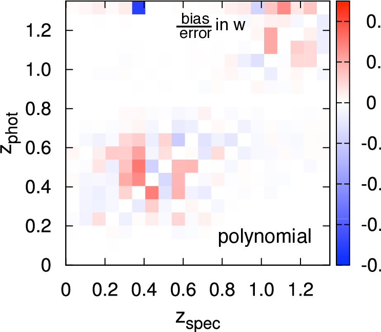
Now we are ready to examine Patch 37. The examination consists of two steps. In step 1, we look into how the differences between the overall redshift distribution and the redshift distribution of Patch 37 affect the estimation of the error distribution for the polynomial and template methods. In step 2, we look at how the errors in the estimation of in any given bin propagate to biases in the dark energy equation of state .
- •
Step 1: Patch 37 redshift biases. Fig. 6 shows the spectroscopic redshift distribution of the whole survey (i.e. of the photometric sample) in black color, as well as that of Patch 37, , in blue (gray). The deviations of the redshift distribution of Patch 37 from that of the full survey directly affect the estimation of , regardless of photo-z method. The top-row panels of Fig. 7 show the difference of for the full sample and Patch 37 (the calibration sample) for the polynomial method (top left) and template method (top right). Comparing Fig. 6 to the top-row panels of Fig. 7, we see that each downward fluctuation of relative to translates into a negative for the corresponding column regardless of photo-z method used. The converse is also true: if overestimates at a given bin, then will be biased high in that column as well.
- •
Step 2: Patch 37 biases in . The bottom-row panels of Fig. 7 show the corresponding fractional biases in the dark energy equation of state in each (,) bin. For each bin, the fractional bias in is essentially a product between the sensitivity in fractional bias to unit redshift errors (shown in Fig. 6) and the actual redshift bias (shown in the left-column panels of Fig. 7 for the two photo-z methods). Even though the sensitivities for fixed contamination are smallest near the diagonal, the actual values of are largest near the diagonal. Overall, the latter effect wins, as the right panels of Fig. 7 show, and the biases in are contributed largely – though not exclusively – by errors near the diagonal, . A noticeable exception is the bin near , , in the polynomial results (left column). Overall, the contribution of this bin lowered the overall fractional bias in , which turns out to be for the polynomial method and 0.52 for the template method. Hence, if it wasn’t for the big negative bias in that bin, the polynomial would have lost to the template method in this patch! The conclusion is that the final bias is the result of several cancellations, which reduce the importance of the choice of photo-z method. However, it is desirable that photo-zs be accurate because it implies that the will more diagonal, which, for comparably stable methods, implies smaller biases in . And perhaps most importantly, better photo-z’s imply better fiducial constraints, which our analysis is not sensitive to.




5.3.2 Statistics of the biases in
In this Section we examine statistics of the biases in when different patches are used for training and/or calibration of the photo-zs. Fig. 8 shows the distribution of the fractional biases when using the and template-fitting estimators as a function of the biases obtained when the polynomial technique is used. The top panel shows the LSS case, and the bottom plot shows the random equivalent. Clearly, biases in introduced by sample variance for the different methods are very correlated while those introduced by Poisson fluctuations alone are not. This suggests that one cannot reduce the effects of sample variance by simply combining estimates based on different photo-z methods.
In Table 2, we show the mean fractional bias in the equation of state , its statistics, and the median total shift in chi-squared (defined below) corresponding to the full-dimensional cosmological parameter space. We define as the range encompassing 68% of the area of the distribution of , where is the bias in the equation of state in any given patch and is the marginalized statistical error in the equation of state. Moreover, we define the total chi-square as
| (20) |
where is a six-dimensional vector containing cosmological parameter biases and is the (statistical-only) Fisher matrix defined in Eq. (15). We then define to be the median of the distribution of .
We find that the distribution of fractional biases are typically reasonably Gaussian, in the sense that our definition of matches the standard deviation of the fractional bias distribution (without the absolute value) to a few percent, and an equivalent definition of is quite close to twice the standard deviation. In Sec. 7, we will assume the distribution of fractional biases is Gaussian to estimate follow-up requirements for the DES survey.
Actual spectroscopic calibration samples should be comprised of several sets of patches of sky. Ideally, the patches should be separated enough so as to be statistically independent. Because of the small size of our simulation it is not possible to combine many independent patches; recall, our simulation covers only on a side. As a simple alternative, we combine several randomly selected patches to create the spectroscopic training and calibration sample. We consider two scenarios, one comprised of patches 120 of with each galaxy selected with probability of 0.03125 - with average total of galaxies. The other scenario is comprised of 180 patches of with galaxies selected with probability 0.125, and with the average total of galaxies. We repeat the procedure for generating these combined samples several times to generate the statistics shown in Table 3.
The point we want to make is that, in the more realistic scenarios with calibration samples coming from separate patches, all of the photo-z methods we tested yield very similar results. Combining patches randomly is far from ideal, hence the bias statistics presented in Table 3 are pessimistic. We consider the spectroscopic requirements with optimal patch selection in Sec. 7.
The conclusions of this Section are:
- •
The LSS and random-equivalent cases lead to very different bias statistics. Conversely, differences between the photo-z methods do not affect the bias statistics considerably. In particular, when many patches are combined, the photo-z estimators perform nearly identically.
- •
The method is the most sensitive to sample variance. This is expected because it is a purely density-based estimator, and it degrades the fastest as the area and size of the training set decrease. However, comparing the statistics of the for different areas in the random equivalent cases suggests that the estimator is not as sensitive to shot noise. Moreover, the method is the only method that yields a perfect reconstruction of the overall redshift distribution in the limit of large area of spectroscopic samples.
- •
The polynomial-fitting method appears to have slightly larger mean fractional bias than the and template-fitting in the cases shown in Table 2. However, the mean fractional bias is significantly smaller than the width in all cases. In addition, the polynomial technique outperforms the other methods in almost all scenarios, suggesting that use of a training set yields improvements superior to any bias introduced by using the same patch to train and calibrate the photo-zs. We believe that the conclusion that one can use the same sample to train and calibrate photo-zs should hold for other training-set-dependent photo-z techniques provided the method has some control for the degrees of freedom it utilizes and thereby avoid biases due to over-fitting.


| Bias in w | ||||||
|---|---|---|---|---|---|---|
| LSS | Random | |||||
| Technique | ||||||
| Template | 0.04 | 2.56 | 3.14 | 0.04 | 0.44 | 0.14 |
| Polynomial | -0.07 | 1.53 | 2.04 | -0.04 | 0.39 | 0.12 |
| 0.05 | 2.33 | 2.56 | 0.07 | 0.31 | 0.10 | |
| .addddaaaaaaa | aaaddddaaaaaa | |||||
| Template | -0.04 | 3.75 | 7.36 | 0.01 | 0.92 | 0.75 |
| Polynomial | -0.19 | 2.96 | 4.74 | 0.00 | 0.93 | 0.64 |
| -0.01 | 3.99 | 9.05 | 0.029 | 0.78 | 0.50 | |
| .addddaaaaaaa | aaaddddaaaaaa | |||||
| Template | 0.03 | 4.61 | 16.4 | -0.15 | 1.9 | 2.9 |
| Polynomial | -0.11 | 3.99 | 10.3 | -0.17 | 1.7 | 2.2 |
| 0.07 | 5.88 | 32.3 | -0.10 | 2.0 | 3.0 | |
| Bias in w (combined random patches) | |||
|---|---|---|---|
| - fraction = 0.03125 | |||
| 120 patches - | |||
| Technique | |||
| Template | 0.12 | 0.84 | 0.59 |
| Polynomial | -0.16 | 0.76 | 0.54 |
| 0.05 | 0.84 | 0.54 | |
| - fraction = 0.125 | |||
| 180 patches - | |||
| Technique | |||
| Template | 0.19 | 0.76 | 0.41 |
| Polynomial | -0.10 | 0.62 | 0.29 |
| 0.12 | 0.74 | 0.39 | |
5.4 Dependence on simulations and parametrizations
In this section we discuss some of our choices of survey parameters.
5.4.1 Dependence on intrinsic ellipticity
For most of the results shown on this paper, we have assumed the optimistic value of for the rms intrinsic ellipticity. The effective intrinsic ellipticity is somewhat difficult to estimate before the survey has started taking data, and there is a range of forecasted values in the literature; for example, (Laszlo et al., 2011; Kirk et al., 2011). We tested using rms ellipticity of 0.26 with the template photo-zs, and found that the change affects primarily the fiducial constraints, degrading e.g. marginalized error in by a factor of (from 0.035 to 0.055). The overall degradation in the of the distribution of degrades by a factor of for the LSS cases and for the random equivalent cases. Since we find that the intrinsic galaxy ellipticity primarily affects the fiducial cosmological parameter errors (i.e. , rather than the systematic bias ), we use it as a control parameter to vary our baseline cosmological parameter error assumptions88 8 Note, it would not be hard to come up with other ways to improve the fiducial constraints, such as adding other 2-pt correlations to the analysis, or including magnification. Conversely, one could add intrinsic alignments and other sources of errors to degrade the constraints.. Henceforth, we adopt as the optimistic case for the dark energy fiducial errors (which leads to more challenging follow-up requirements), and as the pessimistic error case (which leads to more relaxed requirements). Unless mentioned otherwise, results assume the former, optimistic case.
5.4.2 Dependence on redshift range
After the completion of the paper, we obtained a newer version of the DES simulations that reached . We found that the redshift range only comprised about of the sample and had little impact on the results despite the significantly worse photo-zs for galaxies in that range. Fractional biases degrade by , an effect driven primarily by the improvement in fiducial constraints - which assume perfect photo-zs.
5.4.3 Dependence on number of tomographic bins
We have adopted a rather aggressive redshift slicing as our baseline case, assuming 20 tomographic redshift bins distributed in the range. We expect that with fewer redshift slices, photo-z errors will be less pronounced while the statistical errors will increase slightly; and thus that the spectroscopic follow-up requirements derived in this paper will be somewhat relaxed. This expectation is backed up by numerical checks that we now describe.
In addition to , we also consider cases of , 10, 15, 30 and 40 tomographic bins using alternately the template and polynomial photo-z methods. We find that the dependence of biases in cosmological constraints on the number of bins is rather weak. As increases from 5 to 20, the bias in the dark energy equation of state decreases by and converges at this point, not increasing appreciably for higher (reflecting the fact that such small-redshift-scale fluctuations are not degenerate with cosmological information). Moreover, as increases from 5 to 20, the statistical errors on decrease by 10%, and drop a further as is increased to 40. Therefore the bias-to-error ratio decreases by a total of up to but then increases by for . Given these unremarkable dependencies for such a wide range of , and the fact that higher implies more stringent requirements, we conclude that 20 tomographic bins is indeed a good representative choice for the calculations in this paper.
6 Discussion: Can things be improved?
In this section, we discuss possibilities for reducing the impact of sample variance. In Sec. 6.1, we present tests we have performed and in Sec. 6.2 we discuss other possibilites that should be explored.
6.1 Performed tests
- •
Culling: We used the width of the as a criterion to identify catastrophic photo-zs. We removed all galaxies for which , which culled of the galaxies in our simulation. The impact of this selection is summarized in Table 4. The scatter in the photo-zs improved by and for the template and polynomial methods, respectively, and the mean width improved . The width of the fractional bias distribution, as described by improved by and for the polynomial and techniques, respectively, but only improved the template estimator results by the negligible .
We also tried to perform the culling using an error estimate from the template-fitting code99 9 The error estimate we use is the difference between the Z_BEST68_HIGH and Z_BEST68_LOW outputs of the LePhare code.. The results are in the entry Template*, in Table 4. We see that the template error estimation was less efficient than the width for improving the photo-z scatter. With the same fraction of objects removed, the mean scatter improved by only compared to when the width was used. In addition, the culling actually resulted in worsening of the bias in , despite an improvement in the overall cosmological parameter fit measured by the improvement in the median .
The conclusion is that culling of outliers does not seem to be a very efficient way to improve the bias due to photo-z calibration even when it works reasonably well in improving the mean photo-z scatter.
- •
: If the true redshift distribution of the photometric sample is known somehow (e.g. using cross-correlation techniques (Newman, 2008), or from theoretical priors), then one can use it to improve results. As discussed in Sec. 5.1, the quantity is much less sensitive to sample variance than . If for the photometric sample is known, we use the fact that
(21) to estimate from . Table 5 shows the improvement in the statistics of the dark energy equation of state bias. For the case, we see from the last column that the statistics from template-fitting and methods improve by a factor of relative to the fiducial results shown in Table 2; this corresponds to 25 times smaller follow-up samples needed to achieve the same calibration! Improvements for the are not as pronounced, but are still substantial. These results are idealized, because the redshift distribution is assumed to be perfectly known. How well does neeed to be known for this technique to be useful is an open question.
If one uses a estimator (from any algorithm), the s can be corrected using the improved . The ability to correct the redshift estimates is only possible for estimators but not for single-value photo-zs.
6.2 Other possible improvements
In this section we briefly describe potentially interesting techniques to reduce the spectroscopic follow-up requirements, but that go beyond the scope of this paper.
- •
Smoothing, fitting and deconvolution. With enough theoretical priors, one may use assumptions about smoothness or a functional form of the overall redshift distribution to fit the weights estimate of the redshift distribution. Alternatively, since the redshift sample variance is due to the projection along the line-of-sight of the linear power spectrum, one can perhaps use Fourier techniques to deconvolve the large-scale-structure from the redshift distribution estimates.
- •
Repeat observations. The use of repeat photometric observations would help reduce the shot-noise component of the photo-z training procedure. Unfortunately, the sample variance would not be affected. The reduction of such noise might be relevant to help stabilize deconvolution techniques.
| Bias in w (with culling) | ||||||
|---|---|---|---|---|---|---|
| Technique | ||||||
| Template | 0.01 | 2.48 | 3.20 | 0.87 | 0.97 | 1.02 |
| Template* | -0.06 | 2.90 | 2.59 | 0.92 | 1.13 | 0.82 |
| Polynomial | -0.17 | 1.44 | 1.75 | 0.85 | 0.94 | 0.86 |
| 0.03 | 2.08 | 1.94 | 0.90 | 0.89 | 0.75 | |
| Bias in w (with ) | |||||
| Technique | Mean | ||||
| Template | -0.06 | 0.52 | 0.36 | 0.20 | 0.11 |
| Polynomial | -0.13 | 0.87 | 0.43 | 0.57 | 0.21 |
| -0.14 | 0.52 | 0.34 | 0.22 | 0.13 | |
| Template | -0.17 | 1.28 | 1.39 | 0.34 | 0.19 |
| Polynomial | -0.39 | 1.31 | 1.69 | 0.44 | 0.36 |
| -0.29 | 0.98 | 1.14 | 0.25 | 0.13 | |
7 Guide for observing proposals
In this section we provide a guide for observers to determine what observing requirements are needed for photo-z calibration given a specific telescope’s effective angular aperture, number of spectroscopic fibers and collecting area. Typically, calibration requirements have been represented in terms of total number of galaxies. We argue that calibration requirements should be phrased in terms of variables more closely related to total observing time or cost. With this purpose in mind, we define the number of pointings, , to be the product of the number of patches times the number of repeat observations of each patch. For constant collecting area, the number of pointings is a direct measure of total observational time required.
The previous sections focused on calibration requirements from a single patch. If independent patches are combined, the requirements decrease with the square-root of the number of independent patches. This square-root scaling only applies exactly to the template-fitting method because it does not use a training procedure. For simplicity, and because the previous results were rather insensitive to photo-zs, we only use the template photo-zs in this section.
As an example, we consider the case of the Dark Energy Survey. To reach reasonable spectroscopic completeness at the limiting magnitudes of the DES requires very large telescopes. We thus tune our guide to two of the telescopes that will be available for the calibration: VIMOS-VLT and IMACS-Magellan. VLT is an 8-meter class telescope with angular aperture of (or about ). Magellan is a 6.5-meter class telescope with collecting area of . We assume that in each observation, VLT and Magellan can observe about 300-500 galaxies if a low-dispersion setting is used. In real observations, the need to disperse the spectra in the focal plane reduces much of the available collecting area. This is not a random reduction, however. Roughly speaking, spectra cannot be at the edges of the focal plane so that there is room left in the focal plane to disperse the spectra. The design of VLT already accounts for this, but for Magellan there is a loss of up to a half of the total area. To roughly cover the possibilities for existing telescopes of large angular aperture we perform our tests assuming , and fields-of-view.
Fig. 9 shows the number of independent patches that must be observed as function of the number of galaxies per patch so that the photo-z calibration leads to bias in that is smaller than the statistical error in with probability. One can see that, for fixed number of galaxies per patch, the larger the telescope, the smaller the number of independent patches that need to be observed. Hence, assuming equal throughput and same number of available fibers, a telescope such as Magellan is more efficient than VLT for spectroscopic calibration. For reference, we also show the results assuming the full field-of-view of Magellan is available for spectroscopy. For the case of the collecting area, if the telescope can observe 400 galaxies at once, then about 140 independent patches – or a total of galaxies – would be needed to ensure, with probability that the bias in the equation of state is less than the statistical error (i.e. bias/error ). The requirement increases to about 150 and 180 patches for effective angular apertures of and . The requirement for VLT would be about 165 patches (not shown).
The contours in Fig. 9 were constructed by varying the mean fraction of galaxies that are sampled from each patch. The right tip of each contour line corresponds to using of the galaxies in a patch. For a fixed angular aperture, the total number of galaxies required decreases with decreasing sampling fraction. By sampling less galaxies per patch one more efficiently beats down the sample variance, up to the point where shot noise dominates. The total number of galaxies required can never be smaller than the requirements from shot-noise only estimates. In our case, this is about galaxies. The upturn in the contours at low sampling fraction indicates the shot-noise domination regime, at which point reducing the number of galaxies per patch yields no benefit.
How does one use Fig. 9 to deduce more stringent requirements on dark energy parameter biases, or implement different survey assumptions? The distribution of fractional bias in is roughly Gaussian, hence to get - requirements on the bias, one can simply multiply the - requirement plotted by . For example, the requirement of keeping the bias/error less than at - roughly implies that the bias is less than at -. One can use a square-root scaling to deduce more stringent requirements; for example, if one would like the bias/error in to be less than at -, then the number of independent patches required increases by four. Because the effect of the independent number of patches is only a square-root, it is well worth investigating techniques that decrease the sensitivity to the sample variance. For example, as we saw in Sec. 6, if the redshift distribution of the phometric sample could be perfectly known, the calibration biases would decrease by factors of up to 5 which would decrease the number of patches required for photo-z calibration by more than a factor of 25!
Finally, recall that usage of a more realistic intrinsic galaxy ellipticity of 0.26 increases the fiducial error by a factor of 1.6 (from 0.035 to 0.055) and leaves the biases in largely unaffected, resulting in the decreased follow-up requirements by a factor of in the number of patches required. Nevertheless, we think that usage of the smaller value of the intrinsic rms ellipticity used throughout is preferred, given that the fractional biases could be larger than expected. This could happen in two ways: either the fiducial error could be improved by other weak lensing techniques (3-point function, other cross-correlations, etc), or additional systematics might increase the bias . We therefore erred on the side of being conservative in terms of the spectroscopic follow-up requirements, and adopted , or . Our best current understanding is that only three kinds of systematics would increase spectroscopic follow-up requirements: non-random spectroscopic failures, imperfect star-galaxy separation, and variability in observing conditions. Other systematics would likely only cause a degradation in the fiducial cosmological parameter constraints, thereby decreasing follow-up requirements.
The time required for completing observations depends on the requirements on spectroscopic completeness. If we assume that a completeness level comparable to that of the VIMOS-VLT Deep Survey1010 10 http://cesam.oamp.fr/vvdsproject/ (VVDS) is sufficient1111 11 The VVDS-DEEPS survey obtained redshifts for about of their sample with confidence above , and of these, about had confidence of (Le Fèvre et al., 2005) , then two patches of sky can be covered per night using VLT or Magellan, if a single pointing is required per patch. In the absence of spectroscopic failures, the ideal strategy is clearly to use a single pointing per patch to beat down sample variance as fast as possible. However, spectroscopic failures typically cannot be ignored, which makes it harder to determine the optimal observing strategy. The key difficulty is that spectroscopic failure rates vary strongly with galaxy type, which implies that different observing times are needed for different types of galaxies to yield reliable redshifts. In addition, for a fixed galaxy type, there is a broad distribution of intrinsic luminosities. An optimized survey would, at the very least, require a carefully weighted target selection function to ensure the final spectroscopic sample is a representative subsample of the full photometric survey. At best, the ideal survey would combine several telescopes, each optimized for a certain depth and galaxy population. For example, planned surveys such as BigBOSS1212 12 http://bigboss.lbl.gov/ and DESpec1313 13 http://eag.fnal.gov/DESpec/Home.html will have very wide fields of view and be able to obtain several thousand spectra per pointing. An interesting strategy would be to use these telescopes – perhaps with massive coaddition of images – to obtain a large sample to depths slightly brighter than , for galaxy types with more easily detectable spectra. This way, an 8-m class telescope could concentrate exclusively on the very faintest galaxies.
In a forthcoming follow-up to this paper, we incorporate a simulated spectroscopic pipeline to our analysis to determine the levels of spectroscopic completeness that are required for dark energy studies.

8 Conclusions
We used cosmological N-body simulations populated with galaxies with DES photometry to investigate the impact of shot-noise and sample variance in the spectroscopic observations necessary to train the photo-zs and calibrate their error distributions. Our conclusions are as follows:
- •
For typical spectroscopic surveys, sample variance is much larger than shot noise.
- •
Sample variance affects the spectroscopic properties more strongly than photometric properties. Consequently, the error distribution is much more sensitive to sample variance than . Unfortunately, for cosmological analysis is the error distribution that we have to use, which results in calibration requirements that are quite demanding. If the overall distribution of the photometric sample is known somehow, e.g. using cross-calibration techniques, then one can estimate from , which can reduce follow-up requirements by more than an order of magnitude. In addition, if one uses s instead of single-number photo-z estimates, the improved estimate can be used to correct and improve the s.
- •
The use of the same spectroscopic sample to train photo-zs and calibrate the photo-z error distribution does not introduce additional cosmological biases. In addition, the scatter in the photo-zs is, on average, not degraded by sample variance.
- •
For small training sets the method is the most affected by sample variance because it is a pure density estimator (cf. Fig. 3). Conversely, the estimate is the only unbiased method in the sense that, for large enough training, it recovers the true redshift distribution of the photometric sample.
- •
Biases in the dark energy equation of state obtained from the different photo-z methods are highly correlated for sample-variance-dominated calibration samples, suggesting that a simple combination of photo-z methods cannot reduce the biases. Conversely, for shot-noise dominated calibration samples, biases are largely uncorrelated.
- •
Culling of catastrophic outliers is not very effective at reducing calibration requirements, with the decrease in the bias in being comparable to degradation of the statistical errors due to the reduction of the sample size.
- •
We provide a guide to observing proposals of spectroscopic samples directed towards the calibration of photo-zs for the DES. We focus on Magellan and VLT, the two telescopes best suited for DES calibration. To reduce sample variance effects one should spread the observations to as many patches as possible, using as many spectroscopic fibers as possible in each observation. We find that VLT and Magellan would need about 165 and 150 patches respectively in order to ensure, with probability, that the photoz-calibration induced bias in does not dominate its statistical error. This estimate assumes that 400 galaxies can be observed per patch. If a VVDS-level of completeness is sufficient, these observations would require about 85 and 75 nights of observation for VLT and Magellan, respectively, assuming the optimistic fiducial uncertainty of . For a more pessimistic fiducial error , the requirements decrease by a factor of about 3.5. Nevertheless, the former number may be more useful as a guideline, since the overall requirements might be increased by including the type incompleteness and spectroscopic redshift failures, something that we will fully investigate in a forthcoming companion paper.
Acknowledgements
CC would like to thank Joerg Dietrich, Huan Lin, Anja von der Linden and Jeff Newman for discussions about spectroscopic surveys and Stephanie Jouvel for help with the Le Phare code. We thank Gary Bernstein, Joanne Cohn, Martin White, and an anonymous referee for very useful comments. We would like to thank the Kavli Institute for Theoretical Physics in Santa Barbara where some of this work was carried out. MTB and RHW would like to thank their collaborators of the LasDamas project for use of their simulation data. CC and DH are supported by the DOE OJI grant under contract DE-FG02-95ER40899. CC is also supported by a Kavli Fellowship at Stanford University. DH is additionally supported by NSF under contract AST-0807564, and NASA under contract NNX09AC89G. RHW recieved support from the U.S. Department of Energy under contract number DE-AC02-76SF00515. MTB was supported by Stanford University and the Swiss National Science Foundation under contract 2000 124835/1. This research was supported in part by the National Science Foundation under Grant No. PHY05-51164.
Appendix A The simulations
The simulated galaxy catalog used for the present work was generated using the Adding Density Determined GAlaxies to Lightcone Simulations (ADDGALS) algorithm (Wechsler et al., 2012; Busha et al., 2012). This algorithm attaches synthetic galaxies to dark matter particles in a lightcone output from a dark matter N-body simulation. The model is desgined to match the luminosities, colors, and clustering properties of galaxies.
The simulation used here was based on a single “Carmen” simulation from the LasDamas project (McBride et al., 2011). This simulation was run with the publicly available Gadget-2 code and modeled a flat cosmology with and in a 1Gpc/ box with particles. The lightcone output necessary for the ADDGALS algorithm was created by pasting together 33 snapshots in the redshift range . This results in a 220 sq degree lightcone whose orientation was selected such that there are no particle replications in the inner sq. deg. and minimal replications in the outer regions.
The ADDGALS algorithm used to create the galaxy distribution consists of two steps: galaxies based on an input luminosity function are first assigned to particles in the simulated lightcone, after which multi-band photometry is added to each galaxy using a training set of observed galaxies. For the first step, we begin by defining the relation — the probability that a galaxy with magnitude a redshift resides in a region with local density , defined as the radius of a sphere containing of dark matter. This relation can be tuned to reproduce the luminosity-dependent galaxy 2-point function by using a much higher resolution simulation combined with the technique known as subhalo abundance matching. This is an algorithm for populating very high resolution dark matter simulations with galaxies based on halo and subhalo properties that accurately reproduces properties of the observed galaxy clustering (Conroy et al., 2006; Wetzel & White, 2010; Behroozi et al., 2010; Busha et al., 2011). The relationship can be measured directly from the resulting catalog. Once this probability relation has been defined, galaxies are added to the simulation by integrating a (redshift dependent) -band luminosity function to generate a list of galaxies with magnitudes and redshifts, selecting a for each galaxy by drawing from the distribution, and attaching it to a simulated dark matter particle with the appropriate and redshift. The advantage of ADDGALS over other commonly used approaches based on the dark matter halos is the ability to produce significantly deeper catalogs using simulations of only modest size. When applied to the present simulation, we populate galaxies as dim as , compared with the completeness limit for a standard halo occupation (HOD) approach.
While the above algorithm accurately reproduces the distribution of satellite galaxies, central objects require explicit information about the mass of their host halos. Thus, for halos larger than , we assign central galaxies using the explicit mass-luminosity relation determined from our calibration catalog. We also measure for each halos, which is used to draw a galaxy from the integrated luminosity function with the appropriate magnitude and density to place at the center.
For the galaxy assignment algorithm, we choose a luminosity function that is similar to the SDSS luminosity function as measured in Blanton et al. (2003), but evolves in such a way as to reproduce the higher redshift observations of the NDWFS and DEEP2 observations. We use a Schechter Function with , , and , where is the cosmological expansion factor.
Once the galaxy positions have been assigned, photometric properties are added. We begin with a training set of spectroscopic galaxies and the simulated set of galaxies with -band magnitudes generated earlier. For each galaxy in both the training set and simulation we measure , the distance to the 5th nearest galaxy on the sky in a redshift bin. Each simulated galaxy is then assigned an SED based on drawing a random training-set galaxy with the appropriate magnitude and local density, k-correcting to the appropriate redshift, and projecting onto the desired filters. The kcorrections and projections are performed using the Kcorrect code (Blanton et al., 2003). The construction of the SEDs in Kcorrect is described in Blanton & Roweis (2007).
Differences between the training set and simulated galaxy sample complicate the process of color-assignment. In order to compile a sufficiently large training set, we use a magnitude-limited sample of SDSS spectroscopic galaxies brighter than with . The simulated sample, on the other hand, is a volume-limited sample, spanning a broader redshift range. When measuring we restrict ourselves to neighbors brighter than in the simulation sample, while using all objects in the observational catalog. To mitigate differences in luminosity and redshift, each galaxy is rank ordered according to its density in its redshift bin, and require that objects be in the same percentile bin in each sample rather than having the same the absolute value of . This is similar to the method used in Cooper et al. (2008).
The final step for producing a realistic simulated catalog is the application of photometric errors. While the photometric errors generated here are particular to DES, the algorithm can be generalized for any survey. For each galaxy, we add a noise term to the intrinsic galaxy flux, where the noise is drawn from a Gaussian of width
| (22) |
where is the exposure time, the number of pixels covered by a galaxy, the flux of the sky in a single detector pixel, and is the intrinsic flux of the galaxy. Application of the above relation to objects from the SDSS catalog shows that it is able to faithfully reproduce the reported errors of the survey.
References
- Abdalla et al. (2011) Abdalla F.B., Banerji M., Lahav O., Rashkov V., 2011, Mon. Not. R. Astron. Soc., 417, 1891
- Abdalla et al. (2008) Abdalla F.B. et al., 2008, Mon. Not. Roy. Astron. Soc., 387, 969
- Abrahamse et al. (2011) Abrahamse A., Knox L., Schmidt S., Thorman P., Tyson J.A., Zhan H., 2011, Astrophys. J., 734, 36
- Amara & Refregier (2007) Amara A., Refregier A., 2007, Mon. Not. Roy. Astron. Soc., 381, 1018
- Arnouts et al. (1999) Arnouts S., Cristiani S., Moscardini L., Matarrese S., Lucchin F., Fontana A., Giallongo E., 1999, Mon. Not. R. Astron. Soc., 310, 540
- Bartelmann & Schneider (2001) Bartelmann M., Schneider P., 2001, Phys. Rept., 340, 291
- Behroozi et al. (2010) Behroozi P.S., Conroy C., Wechsler R.H., 2010, Astrophys. J., 717, 379
- Benitez (2000) Benitez N., 2000, Astrophys. J., 536, 571
- Bernstein & Huterer (2010) Bernstein G., Huterer D., 2010, Mon. Not. R. Astron. Soc., 401, 1399
- Blanton & Roweis (2007) Blanton M.R., Roweis S., 2007, Astro. Journal, 133, 734
- Blanton et al. (2003) Blanton M.R. et al., 2003, Astrophys. J., 592, 819
- Bolzonella et al. (2000) Bolzonella M., Miralles J.M., Pelló R., 2000, A&A, 363, 476
- Bordoloi et al. (2010) Bordoloi R., Lilly S.J., Amara A., 2010, Mon. Not. R. Astron. Soc., 406, 881
- Budavári et al. (2000) Budavári T., Szalay A.S., Connolly A.J., Csabai I., Dickinson M., 2000, Astro. Journal, 120, 1588
- Busha et al. (2012) Busha M., Wechsler R. et al., 2012, in preparation
- Busha et al. (2011) Busha M.T., Wechsler R.H., Behroozi P.S., Gerke B.F., Klypin A.A., Primack J.R., 2011, ApJ, in press
- Coe et al. (2006) Coe D., Benítez N., Sánchez S.F., Jee M., Bouwens R., Ford H., 2006, Astro. Journal, 132, 926
- Coleman et al. (1980) Coleman G.D., Wu C.C., Weedman D.W., 1980, Astrophys. J. Supp., 43, 393
- Connolly et al. (1995) Connolly A.J. et al., 1995, Astro. Journal, 110, 2655
- Conroy et al. (2006) Conroy C., Wechsler R.H., Kravtsov A.V., 2006, Astrophys. J., 647, 201
- Cooper et al. (2008) Cooper M.C., Tremonti C.A., Newman J.A., Zabludoff A.I., 2008, Mon. Not. R. Astron. Soc., 390, 245
- Csabai et al. (2003) Csabai I. et al., 2003, Astro. Journal, 125, 580
- Cunha et al. (2009) Cunha C.E., Lima M., Oyaizu H., Frieman J., Lin H., 2009, Mon. Not. R. Astron. Soc., 396, 2379
- Feldmann et al. (2006) Feldmann R. et al., 2006, Mon. Not. R. Astron. Soc., 372, 565
- Firth et al. (2003) Firth A.E., Lahav O., Somerville R.S., 2003, Mon. Not. R. Astron. Soc., 339, 1195
- Gerdes et al. (2010) Gerdes D.W., Sypniewski A.J., McKay T.A., Hao J., Weis M.R., Wechsler R.H., Busha M.T., 2010, Astrophys. J., 715, 823
- Hearin et al. (2010) Hearin A.P., Zentner A.R., Ma Z., Huterer D., 2010, Astrophys. J., 720, 1351
- Hildebrandt et al. (2010) Hildebrandt H. et al., 2010, A&A, 523, A31
- Hoekstra & Jain (2008) Hoekstra H., Jain B., 2008, Annual Review of Nuclear and Particle Science, 58, 99
- Hogg et al. (1998) Hogg D.W. et al., 1998, Astro. Journal, 115, 1418
- Hu (1999) Hu W., 1999, Astrophys. J., 522, L21
- Hu (2002) Hu W., 2002, Phys. Rev., D66, 083515
- Huterer (2002) Huterer D., 2002, Phys. Rev., D65, 063001
- Huterer (2010) Huterer D., 2010, Gen. Rel. Grav., 42, 2177
- Huterer & Linder (2007) Huterer D., Linder E.V., 2007, Phys. Rev., D75, 023519
- Huterer et al. (2006) Huterer D., Takada M., Bernstein G., Jain B., 2006, Mon. Not. R. Astron. Soc., 366, 101
- Huterer & Turner (2001) Huterer D., Turner M.S., 2001, Phys. Rev., D64, 123527
- Ilbert et al. (2006) Ilbert O. et al., 2006, A&A, 457, 841
- Ishak & Hirata (2005) Ishak M., Hirata C.M., 2005, Phys. Rev. D, 71, 023002
- Jouvel et al. (2009) Jouvel S. et al., 2009, A&A, 504, 359
- Kirk et al. (2011) Kirk D., Laszlo I., Bridle S., Bean R., 2011, preprint (arXiv:1109.4536)
- Kitching et al. (2008) Kitching T.D., Taylor A.N., Heavens A.F., 2008, Mon. Not. Roy. Astron. Soc., 389
- Knox et al. (1998) Knox L., Scoccimarro R., Dodelson S., 1998, Phys. Rev. Lett., 81, 2004
- Koo (1999) Koo D.C., 1999, in Astronomical Society of the Pacific Conference Series, pp. 3–+
- Laszlo et al. (2011) Laszlo I., Bean R., Kirk D., Bridle S., 2011, preprint (arXiv:1109.4535)
- Le Fèvre et al. (2005) Le Fèvre O. et al., 2005, A&A, 439, 845
- Lima et al. (2008) Lima M., Cunha C.E., Oyaizu H., Frieman J., Lin H., Sheldon E.S., 2008, Mon. Not. R. Astron. Soc., 390, 118
- Ma & Bernstein (2008) Ma Z., Bernstein G., 2008, Astrophys. J., 682, 39
- Ma et al. (2006) Ma Z., Hu W., Huterer D., 2006, Astrophys. J., 636, 21
- McBride et al. (2011) McBride C. et al., 2011, in preparation
- Munshi et al. (2008) Munshi D., Valageas P., Van Waerbeke L., Heavens A., 2008, Phys. Rept., 462, 67
- Nakajima et al. (2012) Nakajima R., Mandelbaum R., Seljak U., Cohn J.D., Reyes R., Cool R., 2012, Mon. Not. R. Astron. Soc., 420, 3240
- Newman (2008) Newman J.A., 2008, Astrophys. J., 684, 88
- Oyaizu et al. (2008a) Oyaizu H., Lima M., Cunha C.E., Lin H., Frieman J., 2008a, Astrophys. J., 689, 709
- Oyaizu et al. (2008b) Oyaizu H., Lima M., Cunha C.E., Lin H., Frieman J., Sheldon E.S., 2008b, Astrophys. J., 674, 768
- Sheldon et al. (2011) Sheldon E.S., Cunha C., Mandelbaum R., Brinkmann J., Weaver B.A., 2011, preprint (arXiv:1109.5192)
- Sun et al. (2009) Sun L. et al., 2009, Astrophys. J., 699, 958
- van Waerbeke et al. (2006) van Waerbeke L., White M., Hoekstra H., Heymans C., 2006, Astroparticle Physics, 26, 91
- Wadadekar (2005) Wadadekar Y., 2005, Publ. Astron. Soc. Pac., 117, 79
- Wang et al. (2007) Wang D., Zhang Y.X., Liu C., Zhao Y.H., 2007, Mon. Not. R. Astron. Soc., 382, 1601
- Wechsler et al. (2012) Wechsler R.H., Busha M.T. et al., 2012, in preparation
- Wetzel & White (2010) Wetzel A.R., White M., 2010, Mon. Not. R. Astron. Soc., 403, 1072