1Introduction

YITP-11-83

TIT/HEP-614

UTHEP-632

T-functions and multi-gluon scattering amplitudes

Yasuyuki Hatsuda¹¹ 1 hatsuda@yukawa.kyoto-u.ac.jp, Katsushi Ito²² 2 ito@th.phys.titech.ac.jp and Yuji Satoh³³ 3 ysatoh@het.ph.tsukuba.ac.jp

$\rule{0.0pt}{5.16663pt}^{*}\hskip-3.99994pt$ Yukawa Institute for Theoretical Physics, Kyoto University
Kyoto, 606-8502, Japan

$\rule{0.0pt}{5.16663pt}^{†}\hskip-3.99994pt$ Department of Physics, Tokyo Institute of Technology
Tokyo, 152-8551, Japan

$\rule{0.0pt}{5.16663pt}^{‡}\hskip-3.99994pt$ Institute of Physics, University of Tsukuba
Ibaraki, 305-8571, Japan

We study gluon scattering amplitudes/Wilson loops in ${\cal N}=4$ super Yang-Mills theory at strong coupling which correspond to minimal surfaces with a light-like polygonal boundary in AdS₃. We find a concise expression of the remainder function in terms of the T-function of the associated thermodynamic Bethe ansatz (TBA) system. Continuing our previous work on the analytic expansion around the CFT/regular-polygonal limit, we derive a formula of the leading-order expansion for the general $2n$ -point remainder function. The T-system allows us to encode its momentum dependence in only one function of the TBA mass parameters, which is obtained by conformal perturbation theory. We compute its explicit form in the single mass cases. We also find that the rescaled remainder functions at strong coupling and at two loops are close to each other, and their ratio at the leading order approaches a constant near 0.9 for large $n$ .

September 2011

1 Introduction

Gluon scattering amplitudes in ${\cal N}=4$ super Yang-Mills theory are dual to light-like polygonal Wilson loops [1, 2]. The AdS-CFT correspondence enables us to study these amplitudes/Wilson loops at strong coupling by calculating the area of the minimal surfaces in AdS with the same light-like polygonal boundary [1].

The logarithm of the ratio of an amplitude to the tree-level amplitude is expressed as the sum of the Bern-Dixon-Smirnov (BDS) part [3] and the remainder function part [4]. The BDS part, which includes the IR divergent terms, is determined by the recursive structure of the amplitudes [5] and the anomalous dual conformal Ward identities [6]. Due to the dual conformal invariance, the remainder function is a function of the cross-ratios of external momenta and has been shown to exist for $n(\geq 6)$ -point amplitudes [8, 7].

It is important to determine its exact form in order to confirm the AdS-CFT correspondence and study the structure of the amplitudes. At weak coupling, it has been calculated perturbatively in some cases [10, 9, 11, 13, 14, 15, 16, 12]. In particular, Heslop and Khoze proposed the two-loop remainder function for $2n$ -point amplitudes for external momenta in ${\mathbb{R}}^{1,1}$ , whose kinematical configuration corresponds to a null polygon with $2n$ -cusps on the AdS₃ boundary [12]. At strong coupling, the remainder function can be evaluated by the minimal surfaces in AdS with the help of integrability [17, 18, 19, 20, 22, 25, 21, 23, 24]. The cross-ratios of the cusp coordinates corresponding to external momenta therein are expressed in terms of the Y-functions, which satisfy the functional relations called the Y-system [26]. The remainder function is then written by these Y-functions in addition to the free energy associated with the Y-system [19].

Under certain asymptotic conditions, the Y-functions also satisfy the Thermodynamic Bethe Ansatz (TBA) integral equations, which describe finite-size effects of two-dimensional integrable models [27]. Around the small mass parameter/high-temperature/UV limit, which corresponds to regular-polygonal Wilson loops, one can study the free energy as the ground state energy of the dual channel by using the conformal perturbation theory. For the minimal surfaces with a $2n$ -gonal boundary in AdS₃, the TBA equations are those of the homogeneous sine-Gordon (HSG) model [28] with purely imaginary resonance parameters [20]. The relevant CFT in the UV limit is the generalized parafermion theory [29] for ${\rm SU}(n-2)_{2}/{\rm U}(1)^{n-3}$ . Similarly for $m$ -cusp Wilson loops/amplitudes in AdS₄, the TBA equations are those of the HSG model associated with the coset ${\rm SU}(m-4)_{4}/{\rm U}(1)^{m-5}$ [20].

In order to obtain an analytic formula for the remainder function around the CFT point, which is the main subject of this paper, we need to find small (complex) mass expansions of the Y/T-functions. For this purpose, we note that the ratio of the $g$ -function (boundary entropy) [30] obeys the same integral equations as for the T-function [31]. Moreover, the exact $g$ -functions for real small masses are obtained by the boundary and bulk perturbation of the corresponding CFT [32, 31]. Combined with an analytic continuation to complex masses, these give the analytic expansion of the T-functions. The expansion of the Y-functions is obtained thereof, since the Y-functions are written generally as ratios of the T-functions. Together with the expansion of the free energy, the analytic expansion for the remainder function is derived.

In [25], Sakai and the present authors presented a general formalism to obtain the small-mass expansion of the $2n$ -point remainder function for the minimal surfaces in AdS₃ along the above line of argument. In particular, the complete leading-order expansion was obtained for $n=5$ by examining the single mass cases classified in [33] and by using the exact mass-coupling relations in [34, 35]. We also derived for $n=4$ an all-order expansion of the integral representation of the remainder function obtained in [17]. These expressions were compared with the 2-loop formulas. After appropriate normalization [9], the two rescaled remainder functions were found to be very close to but different from each other.

The purpose of this paper is to study analytically the remainder function for the minimal surfaces with a $2n$ -gonal boundary in AdS₃ for general $n$ . We show that the cross-ratios of the cusp coordinates appearing in the remainder function are concisely expressed in terms of the T-functions of the associated TBA system. Using this result, we derive a formula of the leading-order expansion for the general $2n$ -point remainder function at strong coupling. The T-system allows us to encode its momentum dependence in only one function of the mass parameters. We explicitly compute this function in several simplified cases where the TBA system contains only one mass scale. We also compare our strong coupling results with those at two loops. As in the case of $n=4,5$ [9, 25], the rescaled remainder functions [9] are close to each other, and their ratio at the leading order decreases to a constant near 0.9 for large $n$ .

This paper is organized as follows: In section 2, we review some basic properties of the remainder function and the T- and Y-functions related to the minimal surfaces in AdS₃. In section 3, we discuss the relation between the cross-ratios of the momenta and the T-functions. We then present a formula for the remainder function expressed in terms of the T-/Y-functions. In section 4, we discuss the expansion of the remainder function around the CFT point. In section 5, we compute the explicit mass parameter dependence of the leading expansion by using the exact mass-coupling relations in the single mass cases. In section 6, we compare the remainder function at strong coupling with the 2-loop formula. We also discuss the large- $n$ limit of the expansion of the remainder function. We conclude with a summary and discussion for future directions in section 7. Appendix A contains some details about the relation between the T-functions and the cross-ratios for even $n$ .

2 Remainder function for $2n$ -point amplitudes

In this section we introduce the remainder function for the scattering amplitudes with external momenta lying in two-dimensional subspace ${\mathbb{R}}^{1,1}$ , which correspond to minimal surfaces in AdS₃ [17, 19, 20, 23, 25]. In this case, the number of gluons should be even for momentum conservation, and thus the boundary of the minimal surfaces forms a light-like polygon with $2n$ -cusps on the AdS₃ boundary. We label its vertices in the light-cone coordinates as $x_{2k-1}=(x_{k}^{+},x_{k-1}^{-})$ , $x_{2k}=(x_{k}^{+},x_{k}^{-})$ with identification $x^{\pm}_{k+n}=x^{\pm}_{k}$ ( $k=1,\cdots,n$ ). The gluon momenta are given by

\displaystyle 2\pi p_{j}=x_{j+1}-x_{j}.

(2.1)

In conformal gauge, the equations for the minimal surfaces reduce to the generalized sinh-Gordon equation $\partial_{z}\partial_{\bar{z}}\alpha-e^{2\alpha}+|p(z)|^{2}e^{-2\alpha}=0$ for a real scalar $\alpha(z,\bar{z})$ , where $(z,\bar{z})$ are worldsheet coordinates. $p(z)$ is a polynomial of $z$ of order $n-2$ for a $2n$ -sided polygon. It is convenient to define the coordinate $w$ satisfying $dw=\sqrt{p(z)}dz$ in order to study the solution. The area of the minimal surfaces defined by $A=4\int d^{2}ze^{2\alpha}$ is decomposed as

A=A_{\rm sinh}+4\int d^{2}z\sqrt{p\bar{p}},\quad A_{\rm sinh}=4\int d^{2}z(e^{2\alpha}-\sqrt{p\bar{p}}).

(2.2)

In order to calculate the area, it is useful to consider two auxiliary linear differential equations for the left and right spinors in AdS₃, so that the coordinates of a minimal surface are constructed as products of the two spinors. Introducing the spectral parameter $\zeta$ , one can combine these equations into a single linear differential equation. Its compatibility condition turns out to be the SU(2) Hitchin system, which reduces to the above generalized sinh-Gordon equation. For a polynomial $p(z)$ of order $n-2$ , there are $n$ angular regions called the Stokes sectors, where one can define the large and small solutions. The small solution in each sector is uniquely defined up to a factor. Let $s_{j}(z,\bar{z};\zeta)$ be the small solution in the $j$ -th Stokes sector, with the normalized Wronskian

\langle s_{j},s_{j+1}\rangle\equiv{\rm det}(s_{j}\;s_{j+1})=1.

(2.3)

We can extend the index $j$ to take values in integers by analytic continuation of the solutions with respect to $z$ . Since the small solutions $s_{j}$ and $s_{j+n}$ belong to the same Stokes sector, we have $s_{j}\propto s_{j+n}$ . We note that from the ratios of the Wronskians

{\cal X}_{ijkl}(\zeta)={\langle s_{i},s_{j}\rangle\langle s_{k},s_{l}\rangle\over\langle s_{i},s_{k}\rangle\langle s_{j},s_{l}\rangle},

(2.4)

one can calculate the cross-ratios of external gluon momenta as

{\cal X}_{ijkl}(1)={x_{ij}^{+}x^{+}_{kl}\over x^{+}_{ik}x^{+}_{jl}},\quad{\cal X}_{ijkl}(i)={x_{ij}^{-}x^{-}_{kl}\over x^{-}_{ik}x^{-}_{jl}}.

(2.5)

We now define the remainder function from the area (2.2). The term $A_{\rm sinh}$ in (2.2) is finite and up to a constant turns out to be minus the free energy $A_{\rm free}=-F$ of an integrable system, which we will discuss shortly. The constant term is evaluated in the limit where the zeros of the polynomial $p(z)$ are separated far apart and each zero gives the value for the hexagon. The second term in (2.2) diverges since the surface extends to infinity, while a finite part is written in terms of the period integrals on the Riemann surface $w^{2}=p(z)$ . Introducing, e.g., the radial cut-off and subtracting the BDS part from the area, we can obtain the remainder function at strong coupling. Because of the dual conformal symmetry [1, 6, 36], it is a function of the cross-ratios of the external momenta. To find its functional form is the main problem in this subject. The formula of the remainder function at strong coupling is different for odd $n$ and even $n$ due to the monodromy around infinity.

2.1 Remainder function for odd $n$

For odd $n$ the remainder function is

R_{2n}={7\pi\over 12}(n-2)+A_{\rm free}+A_{\rm periods}+\Delta A_{\rm BDS}.

(2.6)

Here $A_{\rm free}$ denotes the free energy part. $A_{\rm periods}$ is defined by

A_{\rm periods}=i\sum_{r=1}^{(n-3)/2}\bigl(\bar{w}_{r}^{e}w^{m,r}-w_{r}^{e}\bar{w}^{m,r}\bigr),

(2.7)

where $w^{e}_{r}=\oint_{\gamma_{r}^{e}}\sqrt{p(z)}dz$ and $w^{m,r}=\oint_{\gamma^{m,r}}\sqrt{p(z)}dz$ are the periods for the electric and magnetic cycles with the canonical intersection form $\gamma_{r}^{e}\wedge\gamma^{m,s}=\delta_{r}^{s}$ . The fourth term is the difference between the BDS formula and a part of the area solving the dual conformal Ward identities:

\Delta A_{\rm BDS}=\frac{1}{4}\sum_{i,j=1}^{n}\log\frac{c_{i,j}^{+}}{c_{i,j+1}^{+}}\log\frac{c_{i-1,j}^{-}}{c_{i,j}^{-}},

(2.8)

where $c^{\pm}_{i,j}$ are the sequential cross-ratios formed by neighboring distances. To represent these, we introduce a notation,

[i_{1},i_{2},i_{3},i_{4},i_{5},\cdots,i_{2k}]^{\pm}\equiv-\frac{x^{\pm}_{i_{2}i_{3}}x^{\pm}_{i_{4}i_{5}}\cdots x^{\pm}_{i_{2k}i_{1}}}{x^{\pm}_{i_{1}i_{2}}x^{\pm}_{i_{3}i_{4}}\cdots x^{\pm}_{i_{2k-1}i_{2k}}},

(2.9)

where $x^{\pm}_{ij}\equiv x_{i}^{\pm}-x_{j}^{\pm}$ . The cross-ratios are then given by¹¹ 1 In the following, we choose the range of the indices $i,j$ so that $|j-i|\leq n$ .

c^{\pm}_{i,j}=\left\{\begin{array}[]{cl}[i,i+1,\cdots,j-1,j]^{\pm},&\mbox{$j-i>0$: odd},\\ \mbox{[}i,i-1,\cdots,j+1,j]^{\pm},&\mbox{$j-i>0$: even},\end{array}\right.

(2.10)

together with $c^{\pm}_{i,j}=c^{\pm}_{j,i}$ and $c^{\pm}_{i,i}=c^{\pm}_{i,i+1}=1$ . The path connecting the vertices runs clockwise for odd $j-i>0$ and counterclockwise for even $j-i>0$ , respectively. In Fig. 1 (a), we show an example of $c_{1,6}^{\pm}$ for $n=7$ .

Refer to caption — Figure 1: Examples of sequential cross-ratios. $c_{1,6}$ for $n=7$ is shown in (a). $c_{2,6}^{aux}$ for $n=8$ is shown in (b). In (c), the dotted and dashed line stand for $c_{1,6}^{left}$ and $c_{1,6}^{right}$ for $n=8$ , respectively. In (d), the dotted and dashed line stand for $d_{1,5}^{left}$ and $d_{1,5}^{right}$ for $n=8$ , respectively. Superscripts $\pm$ are suppressed here for simplicity.

2.2 Remainder function for even $n$

For even $n$ case, the remainder function $R_{2n}$ can be obtained from the double soft limit of the $2(n+1)$ -point amplitudes[23], which is $x^{\pm}_{n+1}\rightarrow x^{\pm}_{1}$ . In this limit, one of the branch point of $\gamma^{m,1}$ is sent to infinity, or equivalently $m_{1}\rightarrow\infty$ with $m_{2}$ kept finite in terms of the mass parameters defined later in (2.33). The remainder function in this case receives contributions from the non-trivial monodromy around infinity and becomes

R_{2n}={7\pi\over 12}(n-2)+A_{\rm free}+A_{\rm periods}+A_{\rm etxra}+\Delta A_{\rm BDS}.

(2.11)

Here $A_{\rm free}$ is the free energy again. The period term $A_{\rm periods}$ is

A_{\rm periods}=i\sum_{r=2}^{(n-2)/2}\bigl(\bar{w}_{r}^{e}w^{m,r}-w_{r}^{e}\bar{w}^{m,r}\bigr),

(2.12)

with the same definition of $w_{r}^{e}$ , $w^{m,r}$ as in the odd $n$ case. The extra term $A_{\rm extra}$ is given by

A_{\rm extra}=-\frac{1}{2}(w_{\rm s}+\bar{w}_{\rm s})\log\gamma_{1}^{R}+\frac{1}{2i}(w_{\rm s}-\bar{w}_{\rm s})\log\gamma_{1}^{L},

(2.13)

where $w_{s}$ describes the monodromy of the small solutions around infinity and is given by

e^{w_{\rm s}+\bar{w}_{\rm s}}=[1,2,...,n]^{+},\quad\quad e^{(w_{\rm s}-\bar{w}_{\rm s})/i}=[1,2,...,n]^{-}.

(2.14)

$\gamma^{L}_{1}$ , $\gamma^{R}_{1}$ are the Stokes coefficients of the associated Hitchin equations, which are given by $\langle s_{0},s_{2}\rangle(\zeta)$ at $\zeta=1,i$ , respectively. Finally, the $\Delta A_{\rm BDS}$ term is given by

\Delta A_{\rm BDS}=\frac{1}{4}\sum_{i,j=1}^{n+1}\log\frac{\hat{c}_{i,j}^{+}}{\hat{c}_{i,j+1}^{+}}\log\frac{\hat{c}_{i-1,j}^{-}}{\hat{c}_{i,j}^{-}}.

(2.15)

Here, $\hat{c}^{\pm}_{i,j}=\hat{c}^{\pm}_{j,i}$ $(i,j,=1,...,n+1;$ mod $n+1)$ are obtained from $c_{i,j}^{\pm}$ for the $2(n+1)$ -point amplitudes by the double soft limit and take the form,

\displaystyle\hat{c}^{\pm}_{i,j}=\left\{\begin{array}[]{ll}c_{i,j}^{aux\,\pm}&(i,j=2,...,n),\\ c_{1,2k}^{left\,\pm}&(i=1,\ j=2k),\\ d_{1,2k+1}^{right\,\pm}&(i=1,\ j=2k+1),\\ c_{1,2k}^{right\,\pm}&(i=n+1,\,j=2k),\\ d_{1,2k+1}^{left\,\pm}&(i=n+1,\,j=2k+1),\end{array}\right.

with $\hat{c}^{\pm}_{i,i}=\hat{c}^{\pm}_{i,i+1}=1$ . $c^{aux\,\pm}_{i,j}=c^{aux\,\pm}_{j,i}$ are the cross-ratios for auxiliary polygons made of the cusp points $\{x_{2}^{\pm},\cdots,x_{n}^{\pm}\}$ :

\displaystyle c^{aux\,\pm}_{i,j}

\displaystyle=\left\{\begin{array}[]{cl}[i,i+1,\ldots,j]^{\pm},&\mbox{$j-i>0$: odd},\\ \mbox{[}i,i-1,\ldots,2,n,\ldots,j]^{\pm},&\mbox{$j-i>0$: even},\end{array}\right.

with $c_{i,i}^{aux\,\,\pm}=c_{i,i+1}^{aux\,\pm}=1$ . $c^{left,right\,\pm}_{1,2k}=c^{left,right\,\pm}_{2k,1}$ and $d^{left,right\,\pm}_{1,2k+1}=d^{left,right\,\pm}_{2k+1,1}$ are the cross-ratios containing the vertex $x^{\pm}_{1}$ , which are given by

$\displaystyle c^{left\,\pm}_{1,2k}$	$\displaystyle=$	$\displaystyle[1,2,\ldots,2k]^{\pm},$
$\displaystyle c^{right\,\pm}_{1,2k}$	$\displaystyle=$	$\displaystyle[1,n,\ldots,2k]^{\pm},$
$\displaystyle d^{left\,\pm}_{1,2k+1}$	$\displaystyle=$	$\displaystyle-[1,n,2,3,\ldots,2k+1]^{\pm},$	(2.25)
$\displaystyle d^{right\,\pm}_{1,2k+1}$	$\displaystyle=$	$\displaystyle-[1,2,n,n-1,\ldots,2k+1]^{\pm},$

and $c_{1,2}^{left\,\pm}=c_{1,n}^{right\,\pm}=1$ . In Fig. 1 (b)-(d), we show examples of $\hat{c}_{i,j}$ for $n=8$ .

2.3 Y-functions and free energy

In order to obtain the remainder function as a function of the cross-ratios (2.5), we still need to compute $A_{\rm free}$ and $A_{\rm extra}$ , and to find the relation between $A_{\rm periods}$ and the cross-ratios. These are achieved by using the associated Y- and T-functions. In this subsection, we consider $A_{\rm free}$ and $A_{\rm periods}$ . $A_{\rm extra}$ is discussed in the next subsection. For a review on the T-/Y-system, see [37] for example.

For our purpose, we first define the T-functions $T_{s}$ ( $s=0,\cdots,n-2$ ) by

T_{2k+1}(\theta)=\langle s_{-k-1},s_{k+1}\rangle(\zeta),\quad T_{2k}(\theta)=\langle s_{-k-1},s_{k}\rangle(e^{{\pi i\over 2}}\zeta),

(2.26)

where $\zeta=e^{\theta}$ is the spectral parameter. From the Plücker relation

\langle s_{i},s_{j}\rangle\langle s_{k},s_{l}\rangle+\langle s_{i},s_{l}\rangle\langle s_{j},s_{k}\rangle+\langle s_{i},s_{k}\rangle\langle s_{l},s_{j}\rangle=0,

(2.27)

the functions $T_{s}(\theta)$ are shown to satisfy the T-system of $A_{n-3}$ -type:

T_{s}\Bigl(\theta+\frac{\pi i}{2}\Bigr)T_{s}\Bigl(\theta-\frac{\pi i}{2}\Bigr)=1+T_{s-1}(\theta)T_{s+1}(\theta),

(2.28)

where $T_{0}=1$ by definition, and one can choose the gauge $T_{n-2}=1$ for odd $n$ . We have also set $T_{-1}=T_{n-1}=0$ , which is in accord with (2.26). We note that this T-system is invariant under a (residual) gauge transformation $T_{s}\to e^{\mu_{s}\cosh\theta}T_{s}$ with $\mu_{s}$ being constants satisfying $\mu_{s+1}+\mu_{s-1}=0$ .

We then define the Y-functions $Y_{s}$ ( $s=1,\cdots,n-3$ ) by using ${\cal X}_{ijkl}$ in (2.4):

Y_{2k}(\theta)=-{\cal X}_{-k,k,-k-1,k+1}(\zeta),\quad Y_{2k+1}(\theta)=-{\cal X}_{-k-1,k,-k-2,k+1}(e^{{\pi i\over 2}}\zeta).

(2.29)

These Y-functions satisfy

Y_{s}(\theta)=T_{s-1}(\theta)T_{s+1}(\theta),

(2.30)

and obey the Y-system,

Y_{s}\Bigl(\theta+\frac{\pi i}{2}\Bigr)Y_{s}\Bigl(\theta-\frac{\pi i}{2}\Bigr)=\Bigl(1+Y_{s-1}(\theta)\Bigr)\Bigl(1+Y_{s+1}(\theta)\Bigr),

(2.31)

Here we have set $Y_{0}=Y_{n-2}=0$ , which is in accord with (2.29). The WKB analysis [38, 19] shows that the Y-functions for the minimal surfaces have the asymptotic behavior,

	$\displaystyle\log Y_{s}(\theta)$	$\displaystyle\sim$	$\displaystyle-{m_{s}\over 2\zeta}\quad\ \,(\zeta\rightarrow 0),$
	$\displaystyle\log Y_{s}(\theta)$	$\displaystyle\sim$	$\displaystyle-{\bar{m}_{s}\zeta\over 2}\quad(\zeta\rightarrow\infty).$		(2.32)

Here, we have introduced the “mass” parameters $m_{s}$ which are given by

m_{2k}=-2Z_{2k},\quad m_{2k+1}=2iZ_{2k+1},

(2.33)

through the period integrals $Z_{s}=-\int_{\gamma_{s}}\sqrt{p(z)}dz$ . The cycles $\gamma_{s}$ are related to the electric and magnetic cycles $\gamma^{e}_{r}$ , $\gamma^{m,s}$ by $\gamma_{2k}=(-1)^{k+1}(\gamma^{e}_{k}-\gamma^{e}_{k+1}),\ \gamma_{2k-1}=(-1)^{k+1}\gamma^{m,k}$ . Their intersection numbers are given by $\gamma_{2k}\wedge\gamma_{2l-1}=\delta_{k,l}+\delta_{k+1,l}$ and $\gamma_{2k}\wedge\gamma_{2l}=\gamma_{2k+1}\wedge\gamma_{2l+1}=0$ . Defining the intersection matrix $\theta_{rs}\equiv\gamma_{r}\wedge\gamma_{s}$ and its inverse $w_{rs}\equiv(\theta^{-1})_{rs}$ , which exits for odd $n$ , the period term $A_{\rm periods}$ takes the form $iw_{rs}Z_{r}\bar{Z}_{s}$ for odd $n$ . In terms of $m_{s}$ , it reads

\displaystyle A_{\rm periods}=\frac{1}{4}\sum_{k=1}^{{(n-3)}/{2}}\sum_{j=k}^{{(n-3)}/{2}}(-1)^{j+k+1}(m_{2j}\bar{m}_{2k-1}+\bar{m}_{2j}m_{2k-1}).

(2.34)

The period term for even $n$ is obtained from $A_{\rm periods}$ for odd $n^{\prime}=n+1$ by the double soft limit:

\displaystyle A_{\rm periods}=\frac{1}{4}\sum_{k=2}^{{(n-2)}/{2}}\sum_{j=k}^{{(n-2)}/{2}}(-1)^{j+k+1}(m_{2k-2}\bar{m}_{2j-1}+\bar{m}_{2k-2}m_{2j-1}).

(2.35)

To derive the integral equations obeyed by the Y-functions, we introduce

\tilde{Y}_{s}(\theta)=Y_{s}(\theta+i\varphi_{s}),

(2.36)

where $\varphi_{s}$ are the phases of the mass parameters,

m_{s}=|m_{s}|e^{i\varphi_{s}}.

(2.37)

In terms of these $\tilde{Y}_{s}$ , the asymptotic behavior (2.32) becomes

\log\tilde{Y}_{s}(\theta)\sim-|m_{s}|\cosh\theta\quad(|\theta|\to\infty).

(2.38)

From the Y-system (2.31), one can then derive the integral equations

	$\displaystyle\log\tilde{Y}_{s}(\theta)$		$\displaystyle=-\|m_{s}\|\cosh\theta+\int_{-\infty}^{\infty}d\theta^{\prime}\biggl[K(\theta-\theta^{\prime}+i\varphi_{s}-i\varphi_{s-1})\log\bigl(1+\tilde{Y}_{s-1}(\theta^{\prime})\bigr)$		(2.39)
			$\displaystyle+\,K(\theta-\theta^{\prime}+i\varphi_{s}-i\varphi_{s+1})\log\bigl(1+\tilde{Y}_{s+1}(\theta^{\prime})\bigr)\biggr],$		(2.39)

where the kernel of the integral is defined by

K(\theta)={1\over 2\pi}{1\over\cosh\theta}.

(2.40)

The integral equations are valid for $|\varphi_{s}-\varphi_{s\pm 1}|<\pi/2$ , and are identified [20] with the TBA equations of the homogeneous sine-Gordon (HSG) model with purely imaginary resonance parameters associated with the coset ${\rm SU}(n-2)_{2}/{\rm U}(1)^{n-3}$ .

Finally, we obtain $A_{\rm free}$ by using $\tilde{Y}_{s}$ :

A_{\rm free}={1\over 2\pi}\int_{-\infty}^{\infty}d\theta\sum_{s=1}^{n-3}|m_{s}|\cosh\theta\log\bigl(1+\tilde{Y}_{s}(\theta)\bigr).

(2.41)

In this formalism, the period and free energy terms are given as functions of $m_{s}$ . These are converted to functions of the cross-ratios through the Y-functions, which are also functions of $m_{s}$ . Consequently, one obtains the remainder function for odd $n$ in terms of the cross-ratios of external momenta.

2.4 T-functions and extra term

To complete the computation of the remainder function for even $n$ , we still need $A_{\rm extra}$ in terms of the cross-ratios or indirectly of the mass parameters. It turns out that this reduces to the computation of the T-functions.

In order to obtain the T-functions, we first note that the asymptotic behavior of $Y_{s}$ in (2.32) and the relation between the Y- and the T-functions (2.30) lead to the asymptotic behavior,

	$\displaystyle\log T_{s}(\theta)$	$\displaystyle\sim$	$\displaystyle-{\nu_{s}\over 2\zeta}\quad\,\,(\zeta\rightarrow 0),$
	$\displaystyle\log T_{s}(\theta)$	$\displaystyle\sim$	$\displaystyle-{\bar{\nu}_{s}\zeta\over 2}\quad(\zeta\rightarrow\infty),$		(2.42)

where $\nu_{s}$ satisfy $m_{s}=\nu_{s-1}+\nu_{s+1}$ . Since $T_{0}=1$ , one has $\nu_{0}=0$ . Similarly to the Y-functions, we then introduce

\tilde{T}_{s}(\theta)=T_{s}(\theta+i\phi_{s}),

(2.43)

where $\phi_{s}$ are the phases of $\nu_{s}$ ,

\nu_{s}=|\nu_{s}|e^{i\phi_{s}}.

(2.44)

In terms of $\tilde{T}_{s}$ , the asymptotic behavior (2.42) reads

\log\tilde{T}_{s}(\theta)\sim-|\nu_{s}|\cosh\theta.

(2.45)

From the T-system (2.28), one can then derive the integral equations

\log\tilde{T}_{s}(\theta)=-|\nu_{s}|\cosh\theta+\int_{-\infty}^{\infty}d\theta^{\prime}K(\theta-\theta^{\prime}+i\phi_{s}-i\varphi_{s})\log\bigl(1+\tilde{Y}_{s}(\theta^{\prime})\bigr).

(2.46)

By solving these equations, one obtains $T_{s}$ as functions of $\nu_{s}$ , which are in turn expressed by $m_{s}$ . For odd $n$ , the gauge $T_{n-2}=1$ implies $\nu_{n-2}=0$ . This gives

\displaystyle\nu_{2i}=\sum_{k=0}^{i-1}(-1)^{k}m_{2(i-k)-1},\quad\nu_{2i+1}=\sum_{k=0}^{(n-5)/2-i}(-1)^{k}m_{2(i+k)+2}.

(2.47)

For even $n$ , the gauge $\nu_{n-2}=0$ is not consistent generally, but $\nu_{1}=0$ is possible instead. With this gauge choice,

\displaystyle\nu_{2i}=\sum_{k=0}^{i-1}(-1)^{k}m_{2(i-k)-1},\quad\nu_{2i+1}=\sum_{k=0}^{i-1}(-1)^{k}m_{2(i-k)}.

(2.48)

In particular $\nu_{n-2}$ is given by

\nu_{n-2}=m_{n-3}-m_{n-5}+\cdots+(-1)^{\frac{n}{2}-2}m_{1}.

(2.49)

Since $Y_{n-2}=0$ , we also have

\displaystyle\log T_{n-2}(\theta)=-{1\over 2}\bigl(\nu_{n-2}e^{-\theta}+\bar{\nu}_{n-2}e^{\theta}\bigr).

(2.50)

Now let us write down the extra term $A_{\rm extra}$ for even $n$ in terms of these T-functions. First, since $T_{n-2}=\prod_{k=0}^{n/2-2}Y^{(-1)^{k}}_{n-3-2k}$ , the monodromy terms in (2.14) are given by

e^{w_{s}+\bar{w}_{s}}=\Bigl(T_{n-2}\Bigl(-{\pi\over 2}i\Bigr)\Bigr)^{(-1)^{n/2+1}},\quad e^{(w_{s}-\bar{w}_{s})/i}=\Bigl(T_{n-2}(0)\Bigr)^{(-1)^{n/2+1}}.

(2.51)

In addition, the Stokes coefficients $\gamma_{1}^{L,R}$ are given through the relations $\gamma_{1}(\zeta)=\langle s_{0},s_{2}\rangle(\zeta)=\langle s_{-1},s_{1}\rangle(e^{\pi i}\zeta)=T_{1}(\theta+\pi i)$ . Putting these together, we find

A_{\rm extra}={(-1)^{{n\over 2}}\over 2}\biggl[\log T_{n-2}\Bigl(-{\pi\over 2}i\Bigr)\log T_{1}\Bigl({3\pi\over 2}i\Bigr)-\log T_{n-2}(0)\log T_{1}(\pi i)\biggr].

(2.52)

By expressing $\nu_{s}$ and $m_{s}$ in terms of the cross-ratios through the Y-functions, one obtains the remainder function for even $n$ as a function of momenta.

2.5 ${\mathbb{Z}}_{2n}$ -symmetry and periodicity of Y-/T-functions

The remainder function is invariant under the cyclic shift of the cusp points $x_{k}\to x_{k+1}$ , or in terms of the light-cone coordinates,

\displaystyle x_{j}^{-}\to x_{j+1}^{+}\,,\quad x_{j}^{+}\to x_{j}^{-}.

(2.53)

This ${\mathbb{Z}}_{2n}$ -symmetry is concisely expressed by the Y-functions as [39],

\displaystyle Y_{s}(\theta)\to Y_{s}\Bigl(\theta+\frac{\pi}{2}i\Bigr).

(2.54)

This symmetry strongly constrains the structure of the remainder function [39, 25]. Moreover, acting with this symmetry twice induces a translation of the light-cone coordinates,

\displaystyle x_{j}^{\pm}\to x_{j+1}^{\pm}.

(2.55)

In the next section, we use this ${\mathbb{Z}}_{n}$ -transformation for representing cross-ratios by the Y-/T-functions.

Another property used in the later sections is the periodicity of the Y-/T-functions. First, from the Y-system (2.31) with the boundary condition $Y_{0}=Y_{n-2}=0$ , one finds the following half-periodicity of the Y-functions:

\displaystyle Y_{s}\Bigl(\theta+\frac{\pi i}{2}n\Bigr)=Y_{n-2-s}(\theta),

(2.56)

where $s=0,\dots,n-2$ . We note that this implies the full periodicity $Y_{s}(\theta+\pi in)=Y_{s}(\theta)$ . One can similarly find the periodicity of the T-functions. For odd $n$ , we have the half-periodicity

T_{s}\Bigl(\theta+{\pi i\over 2}n\Bigr)=T_{n-2-s}(\theta),

(2.57)

where $s=0,\dots,n-2$ . For even $n$ one has to take into account the fact that the rightmost T-function is not generally equal to unity; $T_{n-2}(\theta)\neq 1$ . Then, the T-system (2.28) with the boundary condition $T_{0}=1$ and (2.50) leads to the quasi-periodicity,

\displaystyle T_{s}\Bigl(\theta+\frac{\pi i}{2}n\Bigr)=T_{n-2-s}(\theta)T_{n-2}\Bigl(\theta+\frac{\pi i}{2}(s-2)\Bigr),

(2.58)

where $s=0,\dots,n-2$ and we have used $T_{n-2}(\theta+\pi i)=T_{n-2}^{-1}(\theta)$ . For the periodicities of the Y- and T-systems, see [40] for example.

3 Cross-ratios and T-functions

In the previous section, the remainder function was given in terms of the Y-/T-functions, the mass parameters specifying their asymptotic behavior and the sequential cross-ratios $c_{i,j}^{\pm},\hat{c}_{i,j}^{\pm}$ . In this section, we find that $c_{i,j}^{\pm},\hat{c}_{i,j}^{\pm}$ and hence $\Delta A_{\rm BDS}$ are concisely expressed by the T-functions. This shows that each term in the remainder function is directly represented in the language of the Y-/T-system. Furthermore, it turns out that such a representation enables us to derive an analytic expansion of the remainder function around the CFT limit, beyond numerical analysis or that in the small or large mass limit.

Before going into details, let us summarize our notation. In terms of the bracket introduced in (2.9), the 4-point cross-ratios in (2.5) are given by

\displaystyle[i,j,k,l]^{\pm}=-\frac{x^{\pm}_{jk}x^{\pm}_{li}}{x^{\pm}_{ij}x^{\pm}_{kl}}=-{\cal X}_{iljk}(\zeta),

(3.1)

where $\zeta=1(i)$ for plus(minus) sign.²² 2 The cross-ratio $\chi_{ijkl}\equiv x_{ij}x_{kl}/x_{ik}x_{jl}$ satisfies relations such as $\chi_{ijkl}=\chi_{jilk}=\chi_{klij}$ , $\chi_{ikjl}=1/\chi_{ijkl}$ , $\chi_{lijk}=1-\chi_{ijkl}$ , $\chi_{ijkl}/\chi_{ijkm}=\chi_{lkjm}$ . From the relation between ${\cal X}_{ijkl}$ and the Y-functions (2.29), we then find that

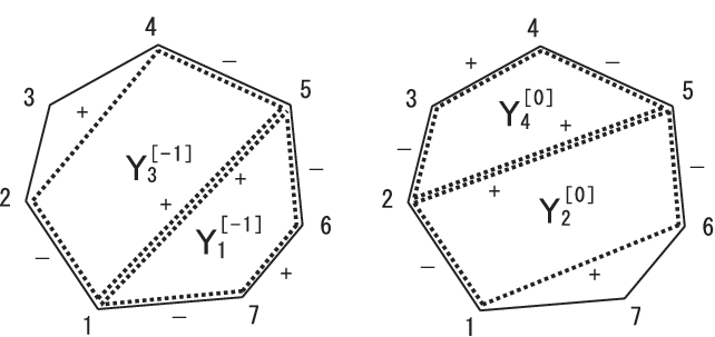
	$\displaystyle[k,k+1,-k-2,-k-1]^{+}=Y_{2k+1}^{[-1]},$		$\displaystyle[k,k+1,-k-1,-k]^{+}=Y_{2k}^{[0]},$
	$\displaystyle{}[k,k+1,-k-2,-k-1]^{-}=Y_{2k+1}^{[0]},$		$\displaystyle[k,k+1,-k-1,-k]^{-}=Y_{2k}^{[1]},$		(3.2)

where

\displaystyle Y^{[k]}_{s}\equiv Y_{s}\Bigl(\frac{\pi i}{2}k\Bigr).

(3.3)

These relations are understood graphically: in the $n$ -gons formed by $x^{\pm}_{i}$ , the Y-functions at special values of $\theta$ are identified with the tetragons which are represented by the brackets in (3.2) . In Fig. 2, we show an example for $n=7$ and $x_{i}^{+}$ .

3.1 Odd $n$ case

Now, let us discuss the relation between the sequential cross-ratios and the Y-/T-functions. We begin with the odd $n$ case, where $c^{\pm}_{i,j}$ are given in (2.10). We recall that the subscripts $i,j$ labeling the vertex are defined modulo $n$ .

To find the relation of our interest, we first derive recursion relations among $c^{\pm}_{i,j}$ . As a simple example, let us consider $c^{+}_{1,n-2}=c^{+}_{1,-2}=[1,0,-1,-2]^{+}=Y_{1}^{[-1]}$ . By adding two vertices, one has $c_{2,-3}=[2,1,0,-1,-2,-3]^{+}$ . Multiplying these two then gives $Y_{3}^{[-1]}$ :

c^{+}_{1,-2}c^{+}_{2,-3}=[1,2,-3,-2]^{+}=Y_{3}^{[-1]}.

(3.4)

This is easily understood graphically as in Fig. 3, where $c_{1,-2}^{+}$ and $Y_{3}^{[-1]}$ are represented as a tetragon whereas $c_{2,-3}$ is as a hexagon. Continuing similar procedures, we also have

c^{+}_{k,-k-1}c^{+}_{k+1,-k-2}=[k,k+1,-k-2,-k-1]^{+}=Y_{2k+1}^{[-1]},

(3.5)

where $k=0,\cdots,r-2$ and we have set $n\equiv 2r+1$ . Another simple example is given by $c^{+}_{r-1,-r+1}=Y_{n-3}^{[0]}$ . Multiplying this with $c^{+}_{r-2,-r+2}$ , we have $c^{+}_{r-2,-r+2}c^{+}_{r-1,-r+1}=Y_{n-5}^{[0]}$ . Similarly, we find

c^{+}_{k,-k}c^{+}_{k+1,-k-1}=[k,k+1,-k-1,-k]^{+}=Y_{2k}^{[0]},

(3.6)

where $k=1,\cdots,r-1$ .

Next, we invert the relations (3.5) and (3.6), to find

	$\displaystyle c^{+}_{k+1,-k-2}$	$\displaystyle\hskip-5.0pt=\hskip-5.0pt$	$\displaystyle\prod_{l=0}^{k}\bigl(Y_{2k+1-2l}^{[-1]}\bigr)^{(-1)^{l}}=T^{[-1]}_{2k+2},$
	$\displaystyle c^{+}_{k,-k}$	$\displaystyle\hskip-5.0pt=\hskip-5.0pt$	$\displaystyle\prod_{l=0}^{\frac{n-3}{2}-k}\bigl(Y_{2k+2l}^{[0]}\bigr)^{(-1)^{l}}=T_{2k-1}^{[0]}.$		(3.7)

These cover all the non-trivial sequential cross-ratios which contain the tetragonal factor $[0,1,-2,-1]^{+}=Y_{1}^{[-1]}$ or $[r-1,r,-r,-r+1]^{+}=Y_{n-3}^{[0]}$ . To obtain other cross-ratios, we use the ${\mathbb{Z}}_{n}$ -transformation $x_{j}^{\pm}\to x_{j+1}^{\pm}$ in (2.55). Since this is generated by $Y_{s}^{[k]}\to Y_{s}^{[k+2]}$ , we find from (3.7) that

	$\displaystyle c^{+}_{k+1+l,-k-2+l}$	$\displaystyle\hskip-5.0pt=\hskip-5.0pt$	$\displaystyle\prod_{l=0}^{k}\bigl(Y_{2k+1-2l}^{[2l-1]}\bigr)^{(-1)^{l}}=T^{[2l-1]}_{2k+2},$
	$\displaystyle c^{+}_{k+l,-k+l}$	$\displaystyle\hskip-5.0pt=\hskip-5.0pt$	$\displaystyle\prod_{l=0}^{\frac{n-3}{2}-k}\bigl(Y_{2k+2l}^{[2l]}\bigr)^{(-1)^{l}}=T_{2k-1}^{[2l]}.$		(3.8)

Graphically, the ${\mathbb{Z}}_{n}$ -transformation generates rotations of the polygons represented by $c_{i,j}^{\pm}$ . The cross-ratios $c_{i,j}^{-}$ are obtained from $c_{i,j}^{+}$ simply by the shift $Y_{s}^{[k]}\to Y_{s}^{[k+1]}$ . We then find that the expression for the cross-ratios are further summarized in the form,

c^{+}_{i,j}=T^{[i+j]}_{|i-j|-1},\quad c^{-}_{i,j}=T^{[i+j+1]}_{|i-j|-1}.

(3.9)

This formula gives a concise expression of $\Delta A_{\rm BDS}$ in (2.8). Furthermore, by using the quasi-periodicity (2.57), one can derive an expression in terms of $T_{s}$ with $s\leq(n-3)/2$ ,

\Delta A_{\rm BDS}=-{1\over 4}\sum_{s=1}^{\frac{n-3}{2}}\sum_{k=1}^{2n}\log\frac{T_{s}^{[k-1]}}{T_{s-1}^{[k]}}\log\frac{T_{s}^{[k]}}{T_{s-1}^{[k-1]}}-{1\over 4}\sum_{k=1}^{n}\log\frac{T_{\frac{n-3}{2}}^{[k-1]}}{T_{\frac{n-3}{2}}^{[k+n]}}\log\frac{T_{\frac{n-3}{2}}^{[k]}}{T_{\frac{n-3}{2}}^{[k+n-1]}},

(3.10)

where $T_{0}=1$ . This is used for studying the expansion of the remainder function in the next section.

3.2 Even $n$ case

Let us move on to the case of even $n$ . In this case, the sequential cross-ratios $\hat{c}^{\pm}_{i,j}$ are generally more complicated than $c^{\pm}_{i,j}$ for odd $n$ . However, it turns out that still $\hat{c}_{i,j}^{\pm}$ are concisely represented by the Y-/T-functions: choosing the range of the indices as $1\leq i,j\leq n+1$ , we find that

	$\displaystyle\hat{c}_{i,j}^{+}$	$\displaystyle\hskip-5.0pt=\hskip-5.0pt$	$\displaystyle\left\{\begin{array}[]{ll}T_{\|i-j\|-1}^{[i+j]}&(\,i-j:\,\mbox{odd}\,)\\ T_{\|i-j\|-1}^{[i+j]}(T_{1}^{[2]})^{(-1)^{j+1}}(T_{n-2}^{[-1]})^{(-1)^{j+\frac{n}{2}}}&(\,i-j:\,\mbox{even}\,)\end{array}\right.\,,$
	$\displaystyle\hat{c}_{i,j}^{-}$	$\displaystyle\hskip-5.0pt=\hskip-5.0pt$	$\displaystyle\left\{\begin{array}[]{ll}T_{\|i-j\|-1}^{[i+j+1]}&(\,i-j:\,\mbox{odd}\,)\\ T_{\|i-j\|-1}^{[i+j+1]}(T_{1}^{[3]})^{(-1)^{j+1}}(T_{n-2}^{[0]})^{(-1)^{j+\frac{n}{2}}}&(\,i-j:\,\mbox{even}\,)\end{array}\right.\,,$

for $2\leq|i-j|\leq n-1$ and $\hat{c}_{i,j}^{\pm}=1$ otherwise. For details, see the appendix. Since the quasi-periodicity (2.58) for even $n$ involves the factor of $T_{n-2}$ , the expression is modified if we choose a different range of $i,j$ . Note also that $(-1)^{j}=(-1)^{i}$ for even $|i-j|$ and the above expression is symmetric with respect to $i$ and $j$ .

This formula gives a concise expression of $\Delta A_{\rm BDS}$ for even $n$ in (2.15). Furthermore, similarly to the case of odd $n$ , one finds an expression in terms of $T_{s}$ with $s\leq(n-2)/2$ by using the quasi-periodicity (2.58) :

$\displaystyle\Delta A_{\rm BDS}$	$\displaystyle=-\frac{1}{4}\sum_{s=1}^{\frac{n}{2}-1}\sum_{k=1}^{2n}\log\frac{T_{s}^{[k-1]}}{T_{s-1}^{[k]}}\log\frac{T_{s}^{[k]}}{T_{s-1}^{[k-1]}}+\frac{1}{2}\sum_{k=0}^{n}\log T_{\frac{n}{2}-1}^{[k]}\log T_{n-2}^{[k+\frac{n}{2}+2]}$
	$\displaystyle\hskip 14.22636pt-\frac{n-1}{4}\log T_{n-2}^{[0]}\log T_{n-2}^{[-1]}+\frac{(-1)^{\frac{n}{2}+1}}{2}\log T_{n-2}^{[-1]}\log T_{1}^{[3]}$	(3.17)
	$\displaystyle\hskip 14.22636pt+\frac{(-1)^{\frac{n}{2}}}{2}\log T_{n-2}^{[0]}\log\Biggl[T_{1}^{[2]}\prod_{l=1}^{[\frac{n}{4}]}(T_{2l-1}^{[0]})^{2(-1)^{l}}\Biggr]$

where $T_{0}=1$ , and $[n/4]$ in the product stands for the greatest integer less than or equal to $n/4$ (Gauss symbol). Since $T_{n-2}(\theta)=e^{-\nu_{n-2}\cosh\theta}$ for real masses, $\log T_{n-2}^{[-1]}$ and hence the middle line in (3.17) vanish in this case.

3.3 Remainder function

Given the expression of $\Delta A_{\rm BDS}$ in terms of the T-functions, the remainder function for the $2n$ -point amplitudes at strong coupling is summarized as follows: For odd $n$ ,

$\displaystyle R_{2n}$	$\displaystyle\hskip-5.0pt=\hskip-5.0pt$	$\displaystyle{7\pi\over 12}(n-2)+{1\over 2\pi}\int_{-\infty}^{\infty}d\theta\sum_{s=1}^{n-3}\|m_{s}\|\cosh\theta\log\bigl(1+\tilde{Y}_{s}(\theta)\bigr)$	(3.18)
		$\displaystyle-{1\over 4}\sum_{k=1}^{(n-3)/2}\sum_{j=k}^{(n-3)/2}(-1)^{j+k}(m_{2j}\bar{m}_{2k-1}+\bar{m}_{2j}m_{2k-1})$
		$\displaystyle-{1\over 4}\sum_{s=1}^{(n-3)/2}\sum_{k=1}^{2n}\log\frac{T_{s}^{[k-1]}}{T_{s-1}^{[k]}}\log\frac{T_{s}^{[k]}}{T_{s-1}^{[k-1]}}-{1\over 4}\sum_{k=1}^{n}\log\frac{T_{(n-3)/2}^{[k-1]}}{T_{(n-3)/2}^{[k+n]}}\log\frac{T_{(n-3)/2}^{[k]}}{T_{(n-3)/2}^{[k+n-1]}},$

For even $n$ , $A_{\rm extra}$ and $\Delta A_{\rm BDS}$ add up to be simplified, and give

$\displaystyle R_{2n}$	$\displaystyle\hskip-5.0pt=\hskip-5.0pt$	$\displaystyle{7\pi\over 12}(n-2)+{1\over 2\pi}\int_{-\infty}^{\infty}d\theta\sum_{s=1}^{n-3}\|m_{s}\|\cosh\theta\log\bigl(1+\tilde{Y}_{s}(\theta)\bigr)$	(3.19)
		$\displaystyle-{1\over 4}\sum_{k=2}^{(n-2)/2}\sum_{j=k}^{(n-2)/2}(-1)^{j+k}(m_{2k-2}\bar{m}_{2j-1}+\bar{m}_{2k-2}m_{2j-1})$
		$\displaystyle-\frac{1}{4}\sum_{s=1}^{\frac{n}{2}-1}\sum_{k=1}^{2n}\log\frac{T_{s}^{[k-1]}}{T_{s-1}^{[k]}}\log\frac{T_{s}^{[k]}}{T_{s-1}^{[k-1]}}+\frac{1}{2}\sum_{k=0}^{n}\log T_{\frac{n}{2}-1}^{[k]}\log T_{n-2}^{[k+\frac{n}{2}+2]}$
		$\displaystyle-\frac{n-1}{4}\log T_{n-2}^{[0]}\log T_{n-2}^{[-1]}+\frac{(-1)^{\frac{n}{2}}}{2}\log T_{n-2}^{[0]}\log\Biggl[\prod_{l=1}^{[\frac{n}{4}]}(T_{2l-1}^{[0]})^{2(-1)^{l}}\Biggr].$

Now the remainder function is written completely in term of the T-/Y-functions. By using these expressions and the conformal perturbation theory of the underlying integrable models, we discuss analytic expansions of the remainder function around the CFT/small-mass limit in the next section .

4 High-temperature expansion

As noted in section 2, the TBA equations (2.39) are identical to those of the homogeneous sine-Gordon model associated with SU( $n-2$ ) ${}_{2}/$ U( $1$ )^n-3. This HSG model is obtained as an integrable perturbation of the coset SU( $n-2$ ) ${}_{2}/$ U( $1$ )^n-3 CFT,

\displaystyle S=S_{\rm CFT}+\lambda\int\!d^{2}x\,\Phi_{\boldsymbol{\lambda},\bar{\boldsymbol{\lambda}}},

(4.1)

where $\Phi_{\boldsymbol{\lambda},\bar{\boldsymbol{\lambda}}}$ is the perturbing operator, which is given by a linear combination of the weight 0 adjoint operators in the coset CFT. The coupling constant $\lambda$ is related to the overall mass scale $M$ as

\displaystyle\lambda=-\kappa_{n}M^{2-(\Delta+\bar{\Delta})},

(4.2)

where $\Delta=\bar{\Delta}=(n-2)/n$ are the conformal dimensions of $\Phi_{\boldsymbol{\lambda},\bar{\boldsymbol{\lambda}}}$ and $\kappa_{n}$ is the dimensionless coupling. In the small-mass limit, one can perturbatively expand the physical quantities around the CFT point ( $\lambda=0$ ) by using the conformal perturbation theory. Since the mass scale is proportional to the inverse temperature, we call it the high-temperature/small-mass expansion. In [25], we discussed the high-temperature expansion in the HSG model. In particular, the Y-/T-functions are expanded by using the relation to the $g$ -function (boundary entropy) [30]. Together with the expansion of the free energy, we obtained the high-temperature expansion of the remainder function at strong coupling for the octagon and for the decagon explicitly.

Here we consider the high-temperature expansion of the remainder function for the general $2n$ -gon at strong coupling. Below we mainly focus on the case that all the masses are real. The results in the general case of complex masses are obtained by complexifying the masses in the final expression [25]. The way of the complexification is specified by consideration based on the ${\mathbb{Z}}_{2n}$ -symmetry (2.54), which is equivalent to $m_{s}\to m_{s}/i$ in the high-temperature expansion.

4.1 Expansion of T-functions

First, let us consider the expansion of the T-function. From the periodicity, the Y- and T-functions have the Laurent expansion for $|\theta|<\infty$ . Each coefficient of the Laurent expansion is further expanded by the scale parameter $l=ML$ near the high-temperature limit, where $L$ is the size of the system. See [25] for detail. In our notation, the mass $M_{j}$ of the $j$ -th particle is related to $m_{j}$ in the TBA equations (2.39) as follows,

\displaystyle|m_{j}|=M_{j}L=\tilde{M}_{j}l,

(4.3)

where $\tilde{M}_{j}\equiv M_{j}/M$ is the relative mass.

For odd $n$ case, since the T-functions satisfy the half-periodicity (2.57), the T-functions are expanded as

\displaystyle T_{s}(\theta)=\sum_{p,q=0}^{\infty}t_{s}^{(p,2q)}l^{(1-\Delta)(p+2q)}\cosh\left(\frac{2p\theta}{n}\right),

(4.4)

with $t_{n-2-s}^{(p,2q)}=(-1)^{p}t_{s}^{(p,2q)}$ . Some of the coefficients $t_{s}^{(p,2q)}$ are fixed by the T-system. For example, one can check that

\displaystyle t_{s}^{(0,0)}=\frac{\sin(\frac{(s+1)\pi}{n})}{\sin(\frac{\pi}{n})},

(4.5)

and

\displaystyle t_{s}^{(1,0)}=t_{s}^{(0,2)}=t_{s}^{(1,2)}=0.

(4.6)

Note that $t_{s}^{(0,0)}$ is equal to the quantum dimensions (ratios of the modular S-matrices) because the T-system reduces to the Q-system at this order. One can also check that (4.5) and (4.6) are consistent with the results from the CFT perturbation. In [25], we determined the first non-trivial coefficient $t_{s}^{(2,0)}$ as

\displaystyle\frac{t_{s}^{(2,0)}}{t_{s}^{(0,0)}}=-\frac{\kappa_{n}G(\tilde{M}_{j})B(1-2\Delta,\Delta)}{2(2\pi)^{1-2\Delta}}\left(\frac{\sin(\frac{3(s+1)\pi}{n})}{\sin(\frac{(s+1)\pi}{n})}\sqrt{\frac{\sin(\frac{\pi}{n})}{\sin(\frac{3\pi}{n})}}-\sqrt{\frac{\sin(\frac{3\pi}{n})}{\sin(\frac{\pi}{n})}}\right),

(4.7)

where $B(x,y)\equiv\Gamma(x)\Gamma(y)/\Gamma(x+y)$ is the beta function, and $G(\tilde{M}_{j})$ is the normalization factor of the two-point function of the perturbing operator $\Phi_{\boldsymbol{\lambda},\bar{\boldsymbol{\lambda}}}$ ,

\displaystyle\Bigl\langle\Phi_{\boldsymbol{\lambda},\bar{\boldsymbol{\lambda}}}(z)\Phi_{\boldsymbol{\lambda},\bar{\boldsymbol{\lambda}}}(0)\Bigr\rangle=\frac{G^{2}}{|z|^{4\Delta}},\qquad G(\tilde{M}_{j})=\sum_{i,j=1}^{n-3}\tilde{M}_{i}^{\frac{2}{n}}F_{ij}\tilde{M}_{j}^{\frac{2}{n}}.

(4.8)

Classically, the coefficients $F_{ij}$ are given by the inverse of the Cartan matrix. At the quantum level, however, these coefficients receive corrections due to the renormalization.

For even $n$ case, the expansion is slightly complicated due to the extra factor in the quasi-periodicity (2.58). From the quasi-periodicity, we find that the T-functions should have the following forms,³³ 3 The quasi-periodicity constrains the form of the exponent up to $(\theta-c_{k})\sinh\theta$ , where $c_{k}$ is a constant. For real masses, the reality condition $\overline{T(\theta)}=T(-\bar{\theta})$ requires $c_{k}=0$ . For $n=4$ with complex masses, this constant is precisely the phase of the mass parameter. One can also check for lower $n$ that $c_{k}$ is independent of $k$ to satisfy the T-system.

	$\displaystyle T_{2k+1}(\theta)$	$\displaystyle=\hat{T}_{2k+1}(\theta)\;e^{(-1)^{k+\frac{n}{2}}\frac{2}{n\pi}\nu_{n-2}\theta\sinh\theta}$		$\displaystyle\left(k=0,\dots,\frac{n}{2}-2\right),$
	$\displaystyle T_{2k}(\theta)$	$\displaystyle=\hat{T}_{2k}(\theta)\;e^{(-1)^{k+\frac{n}{2}}\frac{1}{2}\nu_{n-2}\cosh\theta}$		$\displaystyle\left(k=1,\dots,\frac{n}{2}-2\right).$		(4.9)

Here, $\hat{T}_{s}(\theta)$ satisfy the half-periodicity $\hat{T}_{s}(\theta+\pi in/2)=\hat{T}_{n-2-s}(\theta)$ , and are expanded near the high-temperature limit as

\displaystyle\hat{T}_{s}(\theta)=\sum_{p,q=0}^{\infty}\hat{t}_{s}^{(p,2q)}l^{(1-\Delta)(p+2q)}\cosh\left(\frac{2p\theta}{n}\right).

(4.10)

Since the exponential factors in (4.9) start to be non-trivial at ${\cal O}(l)$ , the coefficients $\hat{t}_{s}^{(p,2q)}$ for lower $p$ and $q$ are the same as $t_{s}^{(p,2q)}$ . Consequently, we have the same formulae (4.5) and (4.6) as in the odd $n$ case, and $\hat{t}_{s}^{(2,0)}=t_{s}^{(2,0)}$ are given by (4.7) for $n\geq 6$ .⁴⁴ 4 For $n=4$ , $\hat{t}_{1}^{(2,0)}$ differs from $t_{1}^{(2,0)}$ due to the factor in (4.9), and (4.7) does not make sense because $\Delta=1/2$ . The relation between the T-function and the $g$ -function, from which (4.7) is derived, is based on the integral equations obeyed by them and not on the particular form of the expansion. One can numerically check (4.7) for even $n$ , as was done for odd $n$ [25]. We also note that $T_{2k+1}(\theta)$ for even $n$ contain the non-analytic term $\log l$ in the high-temperature expansion. This follows from the integral equations (2.46) and the above expansions (4.9). The non-analytic terms are cancelled in $Y_{s}$ and $T_{2k}$ , which are given by the ratios of $Y_{s}$ . We will come to this point later again.

4.2 Expansion of remainder function at strong coupling

Now let us consider the high-temperature expansion of the remainder function at strong coupling. As seen in the previous sections, the remainder function is given by (2.6) or (3.18) for odd $n$ and by (2.11) or (3.19) for even $n$ .

4.2.1 Odd $n$ case

Let us first consider the odd $n$ case. In this case, the period term is given by (2.34). As seen in [25], the CFT perturbation allows us to expand the free energy part as

\displaystyle A_{\rm free}=\frac{\pi}{6}c_{n}+f_{n}^{\rm bulk}+\sum_{k=2}^{\infty}f_{n}^{(k)}l^{\frac{4k}{n}},

(4.11)

where $c_{n}$ is the central charge of the coset CFT for SU( $n-2$ ) ${}_{2}/$ U( $1$ )^n-3, and $f_{n}^{\rm bulk}$ is the bulk contribution. They are given respectively by

\displaystyle c_{n}=\frac{(n-2)(n-3)}{n},\quad f_{n}^{\rm bulk}=\frac{1}{4}\sum_{j,k=1}^{n-3}m_{j}(I^{-1})_{jk}m_{k},

(4.12)

with $I_{jk}$ being the incidence matrix for $A_{n-3}$ . One can check that the bulk term $f_{n}^{\rm bulk}$ just cancels with the period part $A_{\rm periods}$ .⁵⁵ 5 Useful relations to see this are $Z_{j}=-\frac{1}{2}\eta_{jk}m_{k}$ and the one between the incidence matrix and the intersection matrix $I=i\eta\theta\eta^{-1}$ where $\eta=$ diag $(i,1,i,\cdots)$ . The corrections $f_{n}^{(k)}$ in (4.11) are given by the worldsheet integral of the connected $k$ -point function of the perturbing operator. For $k=2$ , we have

\displaystyle f_{n}^{(2)}=\frac{\pi}{6}C_{n}^{(2)}\kappa_{n}^{2}G^{2}(\tilde{M}_{j}),

(4.13)

where

\displaystyle C_{n}^{(2)}=3(2\pi)^{\frac{2(n-4)}{n}}\gamma^{2}\left(\frac{n-2}{n}\right)\gamma\left(\frac{4-n}{n}\right),

(4.14)

and $\gamma(x)\equiv\Gamma(x)/\Gamma(1-x)$ .

Since $\Delta A_{\rm BDS}$ is expressed in terms of the T-functions as in (3.10), we find the high-temperature expansion of $\Delta A_{\rm BDS}$ after substituting (4.4) into (3.10),

\displaystyle\Delta A_{\rm BDS}=-\frac{n}{2}\sum_{s=1}^{(n-3)/2}\log^{2}\left(\frac{t_{s}^{(0,0)}}{t_{s-1}^{(0,0)}}\right)-l^{\frac{8}{n}}\frac{n}{4}\left[\sum_{s=1}^{(n-3)/2}A_{n,s}-2\left(\frac{t_{\frac{n-3}{2}}^{(2,0)}}{t_{\frac{n-3}{2}}^{(0,0)}}\right)^{2}\sin^{2}\left(\frac{\pi}{n}\right)\right],

(4.15)

where

	$\displaystyle A_{n,s}$	$\displaystyle\equiv\left[\left(\frac{t_{s-1}^{(2,0)}}{t_{s-1}^{(0,0)}}\right)^{2}+\left(\frac{t_{s}^{(2,0)}}{t_{s}^{(0,0)}}\right)^{2}\right]\cos\left(\frac{2\pi}{n}\right)-\frac{2t_{s-1}^{(2,0)}t_{s}^{(2,0)}}{t_{s-1}^{(0,0)}t_{s}^{(0,0)}}$
		$\displaystyle\hskip 14.22636pt+\left[\left(\frac{t_{s-1}^{(2,0)}}{t_{s-1}^{(0,0)}}\right)^{2}-\left(\frac{t_{s}^{(2,0)}}{t_{s}^{(0,0)}}\right)^{2}-4\left(\frac{t_{s-1}^{(0,4)}}{t_{s-1}^{(0,0)}}-\frac{t_{s}^{(0,4)}}{t_{s}^{(0,0)}}\right)\right]\log\left(\frac{t_{s}^{(0,0)}}{t_{s-1}^{(0,0)}}\right),$		(4.16)

and we have used (4.6). The coefficients $t_{s}^{(0,0)}$ and $t_{s}^{(2,0)}$ are given by (4.5) and (4.7), respectively. For $t_{s}^{(0,4)}$ , we have the equations which follow from the T-system,

\displaystyle 2t_{s}^{(0,0)}t_{s}^{(0,4)}+\frac{1}{2}(t_{s}^{(2,0)})^{2}\cos\left(\frac{4\pi}{n}\right)=t_{s-1}^{(0,0)}t_{s+1}^{(0,4)}+t_{s+1}^{(0,0)}t_{s-1}^{(0,4)}+\frac{1}{2}t_{s-1}^{(2,0)}t_{s+1}^{(2,0)},

(4.17)

for $s=1,\dots,n-3$ . By solving these equations with the boundary condition $T_{0}=T_{n-2}=1$ , the coefficients $t_{s}^{(0,4)}$ are expressed in terms of $t_{s}^{(0,0)}$ and $t_{s}^{(2,0)}$ .

We note that $t_{s}^{(3,0)},t_{s}^{(2,2)}$ and $t_{s}^{(4,0)}$ do not appear in the expansion. This is understood as a consequence of the ${\mathbb{Z}}_{2n}$ -symmetry: For general complex $m_{s}$ , the terms in the expansion (4.4) are modified [25] as $t_{s}^{(p,2q)}\cosh(2p\theta/n)\to\frac{1}{2}(t_{s}^{(p,2q)}e^{2p\theta/n}+\bar{t}_{s}^{(p,2q)}e^{-2p\theta/n})$ . Under the ${\mathbb{Z}}_{2n}$ -transformation (2.54), these coefficients transform as $(t_{s}^{(p,2q)},\bar{t}_{s}^{(p,2q)})\to(t_{s}^{(p,2q)}e^{p\pi i/n},\bar{t}_{s}^{(p,2q)}e^{-p\pi i/n})$ . Given the vanishing coefficients (4.6) at lower orders, the non-constant combinations invariant under the ${\mathbb{Z}}_{2n}$ -symmetry are only $t_{s}^{{(2,0)}}\bar{t}_{s}^{{(2,0)}}$ and $t_{s}^{(0,4)}$ up to ${\cal O}(l^{\frac{8}{n}})$ .

Combining all of the above results, we then find that the remainder function at strong coupling has the following high-temperature expansion,

\displaystyle R_{2n}=R_{2n}^{(0)}+l^{\frac{8}{n}}R_{2n}^{(4)}+{\cal O}(l^{\frac{12}{n}}),

(4.18)

where

	$\displaystyle R_{2n}^{(0)}$	$\displaystyle=\frac{\pi}{4n}(n-2)(3n-2)-\frac{n}{2}\sum_{s=1}^{(n-3)/2}\log^{2}\left(\frac{\sin(\frac{(s+1)\pi}{n})}{\sin(\frac{s\pi}{n})}\right),$		(4.19)
	$\displaystyle R_{2n}^{(4)}$	$\displaystyle=\frac{\pi}{6}C_{n}^{(2)}\kappa_{n}^{2}G^{2}(\tilde{M}_{j})-\frac{n}{4}\left[\sum_{s=1}^{(n-3)/2}A_{n,s}-2\left(\frac{t_{\frac{n-3}{2}}^{(2,0)}}{t_{\frac{n-3}{2}}^{(0,0)}}\right)^{2}\sin^{2}\left(\frac{\pi}{n}\right)\right].$		(4.20)

Note that the leading term $R_{2n}^{(0)}$ gives the remainder function for the regular $2n$ -gon.

By further using (4.7) and (4.17), the results are expressed by $t_{s}^{(0,0)}$ and, e.g., $t_{1}^{(2,0)}$ . All the mass parameter dependence is encoded in the latter. The results for complex masses are given by replacing $(t_{1}^{(2,0)})^{2}$ in the resultant expression by $t_{1}^{(2,0)}\bar{t}_{1}^{(2,0)}$ . One can also express the result in terms of the expansion coefficients of the Y-function $y_{s}^{(2,0)}$ , which are defined similarly to $t_{s}^{(2,0)}$ , by using the relation,

\displaystyle y_{s}^{(2,0)}=2\cos\Bigl(\frac{2\pi}{n}\Bigr)t_{s}^{(0,0)}t_{s}^{(2,0)}\quad\ (n\geq 5).

(4.21)

4.2.2 Even $n$ case

Let us next consider the even $n$ case. In this case, the period term is given by (2.35). The free energy part is expanded as in (4.11), but the bulk term is now given by [25]

\displaystyle f_{n}^{\rm bulk}=\frac{1}{n\pi}\nu_{n-2}^{2}\log l.

(4.22)

As in (2.52), $A_{\rm extra}$ is expressed by $T_{1}$ and $T_{n-2}$ . It contains the non-analytic term $\log l$ coming from $T_{1}$ , and this is canceled by $f_{n}^{\rm bulk}$ . To see this, let us recall that $L_{1}\equiv\log(1+Y_{1})$ has the following order $l$ term [41]

\displaystyle L_{1}\sim-\frac{2}{n}\nu_{n-2}\cosh\left(\theta+\frac{in\pi}{2}\right)=(-1)^{\frac{n}{2}+1}\frac{2}{n}\nu_{n-2}\cosh\theta.

(4.23)

This term leads to the $\log l$ term in $\log T_{1}$ as

\displaystyle\log T_{1}(\theta_{0})\sim\int_{-\log(1/l)}^{\log(1/l)}\frac{d\theta}{2\pi}\frac{L_{1}(\theta)}{\cosh(\theta_{0}-\theta)}\sim(-1)^{\frac{n}{2}}\frac{2}{n\pi}\nu_{n-2}\cosh\theta_{0}\log l,

(4.24)

where $\theta_{0}$ is a constant. Since $A_{\rm extra}$ reduces to

\displaystyle A_{\rm extra}=\frac{(-1)^{\frac{n}{2}+1}}{2}\log T_{n-2}(0)\log T_{1}(\pi i),

(4.25)

for real masses, we have

\displaystyle A_{\rm extra}\sim-\frac{1}{n\pi}\nu_{n-2}^{2}\log l+{\cal O}(l),

(4.26)

which indeed cancels $f_{n}^{\rm bulk}$ . We also note that the analytic term of $A_{\rm extra}$ starts from order $l$ , because $\log T_{n-2}(0)=-\nu_{n-2}$ is of order $l$ .

For the expansion of $\Delta A_{\rm BDS}$ , we first note that

\displaystyle\log T_{s}(\theta)=\log\hat{T}_{s}(\theta)+{\cal O}(l),

(4.27)

and the exponential factors in (4.9) and $T_{n-2}$ are irrelevant up to ${\cal O}(l^{\frac{8}{n}})$ for $n\geq 10$ . Thus, similarly to the odd $n$ case, $\Delta A_{\rm BDS}$ for $n\geq 10$ is expanded as⁶⁶ 6 As we have mentioned, $\log T_{2k+1}$ contain the non-analytic terms. Such terms, however, do not appear in $\Delta A_{\rm BDS}$ , because $\Delta A_{\rm BDS}$ is originally expressed by the cross-ratios $\hat{c}_{i,j}^{\pm}$ and these cross-ratios can be expressed by the Y-functions only, which do not have the non-analytic terms.

\displaystyle\Delta A_{\rm BDS}=-\frac{n}{2}\sum_{s=1}^{n/2-1}\log^{2}\left(\frac{t_{s}^{(0,0)}}{t_{s-1}^{(0,0)}}\right)-l^{\frac{8}{n}}\frac{n}{4}\sum_{s=1}^{n/2-1}\hat{A}_{n,s}+{\cal O}(l^{\frac{12}{n}}),

(4.28)

where $\hat{A}_{n,s}$ is given by replacing $t_{s}^{(p,2q)}$ in (4.16) by $\hat{t}_{s}^{(p,2q)}$ . These are, however, given by (4.5), (4.7) and (4.17) as in the case of odd $n$ , since $t_{s}^{(p,2q)}=\hat{t}_{s}^{(p,2q)}$ for $p+2q<n/2$ . Combining the relevant terms from $A_{\rm free}$ and $\Delta A_{\rm BDS}$ , we find for $n\geq 10$ that

\displaystyle R_{2n}=R_{2n}^{(0)}+l^{\frac{8}{n}}R_{2n}^{(4)}+{\cal O}(l^{\frac{12}{n}}),

(4.29)

where

	$\displaystyle R_{2n}^{(0)}$	$\displaystyle=\frac{\pi}{4n}(n-2)(3n-2)-\frac{n}{2}\sum_{s=1}^{n/2-1}\log^{2}\left(\frac{\sin(\frac{(s+1)\pi}{n})}{\sin(\frac{s\pi}{n})}\right),$		(4.30)
	$\displaystyle R_{2n}^{(4)}$	$\displaystyle=\frac{\pi}{6}C_{n}^{(2)}\kappa_{n}^{2}G^{2}(\tilde{M}_{j})-\frac{n}{4}\sum_{s=1}^{n/2-1}\hat{A}_{n,s}.$		(4.31)

For $n=4$ , we can obtain the all order expansion in $l$ . The logarithmic terms there are canceled out, and the remainder function is expanded in $l^{2}$ . See [25] for detail. We have also checked that the final results (4.29)-(4.31) are valid for $n=6,8$ : the contributions from the extra factors in the T-functions in (4.9) exactly cancel with those from $A_{\rm extra}$ , so that the final result becomes ${\mathbb{Z}}_{2n}$ -symmetric. The relations (4.5), (4.6), (4.7) and (4.17) also hold.

As in the case of odd $n$ , the results for complex masses are given by expressing $t_{s}^{(2,0)}$ and $\kappa_{n}G$ , e.g., by $t_{1}^{(2,0)}$ and replacing $(t_{1}^{(2,0)})^{2}$ by $t_{1}^{(2,0)}\bar{t}_{1}^{(2,0)}$ (for $n\geq 6$ ). In Table 1 of section 6, we list the numerical values of $R_{2n}^{(0)}$ and $R_{2n}^{(4)}/t_{1}^{(2,0)}\bar{t}_{1}^{(2,0)}$ for both odd and even $n$ . Since the mass-parameter dependence is encoded in $t_{1}^{(2,0)}\bar{t}_{1}^{(2,0)}$ , they are independent of $m_{s}$ and $\kappa_{n}G$ .

4.3 Relation between cross-ratios and mass parameters

In summary, the leading correction to the remainder function around the CFT limit is expressed by the coefficients $t_{s}^{(0,0)}$ , $t^{(2,0)}_{s}$ and $\kappa_{n}G$ , where $\kappa_{n}$ is the dimensionless coupling defined in (4.2) and $G$ is the normalization factor of the two-point function in (4.8). From (4.7), $t_{s}^{(2,0)}$ are also regarded as functions of $\kappa_{n}G$ , and vice versa. Thus, the result is given in terms of (one of) $t_{s}^{(2,0)}$ or $\kappa_{n}G$ , which are functions of the mass parameters.

The momentum dependence of the remainder function is read off through their relation to the Y-functions. Indeed, similarly to $T_{s}$ the Y-functions for general complex masses are expanded near the CFT limit as

\displaystyle Y_{s}(\theta)=y_{s}^{(0,0)}+\frac{1}{2}\Bigl(y_{s}^{(2,0)}e^{{4\over n}\theta}+\bar{y}_{s}^{(0,0)}e^{-{4\over n}\theta}\Bigr)l^{\frac{4}{n}}+{\cal O}(l^{\frac{6}{n}}).

(4.32)

Here, $y_{s}^{(0,0)}$ are the solution to the constant Y-system, $y_{s}^{(0,0)}=\sin\bigl(\frac{s\pi}{n}\bigr)\bigl(\frac{(s+2)\pi}{n}\bigr)/\sin^{2}\bigl(\frac{\pi}{n}\bigr)$ . For real $m_{s}$ , one has $y_{s}^{(2,0)}=\bar{y}_{s}^{(2,0)}$ . From (4.21), we then find that

\displaystyle Y_{s}^{[k]}=y_{s}^{(0,0)}+\cos\Bigl(\frac{2\pi}{n}\Bigr)t_{s}^{(0,0)}\Bigl(t_{s}^{(2,0)}e^{{2\pi\over n}ki}+\bar{t}_{s}^{(2,0)}e^{-{2\pi\over n}ki}\Bigr)l^{\frac{4}{n}}+{\cal O}(l^{\frac{6}{n}}).

(4.33)

By inverting these relations, the remainder function is expressed in terms of the cross-ratios of momenta (which depend on each other at this order through (4.33)). To be concrete, one finds that

	$\displaystyle\|t_{s}^{(2,0)}\|l^{\frac{4}{n}}$	$\displaystyle\hskip-5.0pt=\hskip-5.0pt$	$\displaystyle\frac{\delta Y_{s}^{[0]}}{2t_{s}^{(0,0)}\cos\frac{2\pi}{n}\cos\varphi_{s}}\,,$
	$\displaystyle\frac{2\pi}{n}\varphi_{s}$	$\displaystyle\hskip-5.0pt=\hskip-5.0pt$	$\displaystyle\arctan\biggl(\cot\Bigl(\frac{2\pi}{n}\Bigr)\frac{\delta Y_{s}^{[-1]}-\delta Y_{s}^{[1]}}{\delta Y_{s}^{[-1]}+\delta Y_{s}^{[1]}}\biggr)\,,$		(4.34)

at this order. Here, we have set $t_{s}^{(2,0)}=|t_{s}^{(2,0)}|e^{i\varphi_{s}}$ , and $\delta Y_{s}^{[k]}$ are the deviations of the cross-ratios from the regular-polygonal/small-mass limit, $\delta Y_{s}^{[k]}\equiv Y_{s}^{[k]}-y_{s}^{(0,0)}$ . The cross-ratios are given by (3.1), (3.2) and the ${\mathbb{Z}}_{n}$ symmetry (2.55) or $Y_{s}^{[k]}\to Y_{s}^{[k+2]}$ . From (4.20) and (4.31), it then follows that the remainder function depends on these cross-ratios through $\kappa_{n}^{2}G\bar{G}\ \propto\ |t_{s}^{(2,0)}|^{2}$ given via (4.34). Once $t_{s}^{(2,0)}$ are expressed by $m_{s}$ , one can also find the momentum dependence along the trajectories parametrized by them. The relation between the sequential cross-ratios $c^{\pm}_{i,j},\hat{c}_{i,j}^{\pm}$ and $t_{s}^{(2,0)}$ or $\kappa_{n}G$ is similarly found from the expansion of $T_{s}$ .

5 Mass-coupling relations in single mass cases

As mentioned at the end of the last section, the momentum dependence of the leading expansion of the remainder function is traced through $t_{s}^{(2,0)}$ or $\kappa_{n}G$ by expressing them as functions of the $n-3$ mass parameters $m_{s}$ . In this section, we find the exact form of $\kappa_{n}G$ and hence of $t_{s}^{(2,0)}$ in simple cases where the TBA system has only one mass scale. Such TBA systems associated with various Dynkin diagrams are classified in [33], and our TBA system with a single mass scale reduces to the known ones in the classification [25]. We read off $\kappa_{n}G$ thereof.

The single mass cases discussed below fix $(n-1)/2$ parameters for odd $n$ and $(n-2)/2$ for even $n$ among the $(n-1)(n-3)/4$ independent parameters in $\kappa_{n}G$ for odd $n$ and $(n-2)^{2}/4$ for even $n$ .⁷⁷ 7 There are two symmetries for $F_{ij}$ , $F_{ij}=F_{ji}$ and $F_{ij}=F_{n-2-i,n-2-j}$ , and one can absorb the over all scale into $l$ . For $n=5$ , these single mass cases completely fix the form of $\kappa_{n}G$ [25].

5.1 Case of perturbed unitary minimal model

Let us first consider the case that only the leftmost mass parameter is non-zero:

\displaystyle M_{1}=M,\quad M_{2}=\dots=M_{n-3}=0.

(5.1)

In this case, the TBA equations for the homogeneous sine-Gordon theory reduces to those for the (RSOS)_n-2 scattering theory [42, 43], which is regarded as the massive perturbation of the unitary minimal model ${\cal M}_{n-1,n}$ by the primary field $\Phi_{1,3}$ . Taking into account an appropriate normalization of the overall scale, we then find

\displaystyle\kappa_{n}G(\tilde{M}_{j})=\kappa_{n}F_{11}=\kappa_{n}^{\rm RSOS},

(5.2)

where the constant $\kappa_{n}^{\rm RSOS}$ is given by [42]

\displaystyle\kappa_{n}^{\rm RSOS}=\frac{1}{\pi}\frac{n^{2}}{(n-2)(2n-3)}\biggl[\gamma\Bigl(\frac{3(n-1)}{n}\Bigr)\gamma\Bigl(\frac{n-1}{n}\Bigr)\biggr]^{\frac{1}{2}}\biggl[\frac{\sqrt{\pi}\Gamma(\frac{n}{2})}{2\Gamma(\frac{n-1}{2})}\biggr]^{\frac{4}{n}}.

(5.3)

Although (5.2) and (5.3) have already been given in [25], we have included them for completeness. Given this coupling, we also find that the first non-trivial coefficient (4.13) becomes,

\displaystyle f_{n}^{(2)}=2\pi\left(\frac{n-3}{n-2}\right)^{2}\biggl[\frac{1}{4\sqrt{\pi}}\frac{\Gamma(\frac{n}{2})}{\Gamma(\frac{n-1}{2})}\biggr]^{\frac{8}{n}}\gamma\left(\frac{4}{n}-1\right)\gamma\left(1-\frac{3}{n}\right)\gamma^{2}\left(1-\frac{2}{n}\right)\gamma\left(1-\frac{1}{n}\right).

(5.4)

5.2 Case of perturbed unitary SU(2) diagonal coset model

Let us next consider the case that only the $k$ -th mass parameter is non-zero:⁸⁸ 8 The result in this subsection is based on discussions with Kazuhiro Sakai.

\displaystyle M_{j}=\delta_{jk}M\;\;{\rm for}\;\;j=1,\dots,n-3.

(5.5)

In the following, we take the normalization,

\displaystyle\kappa_{n}G(\tilde{M}_{j})=\kappa_{n}^{\rm RSOS}\sum_{i,j=1}^{n-3}\tilde{M}_{i}^{\frac{2}{n}}\frac{F_{ij}}{F_{11}}\tilde{M}_{j}^{\frac{2}{n}},

(5.6)

which reduces to (5.2) in the previous case, and

\displaystyle\kappa_{n}G(\tilde{M}_{j})=\kappa_{n}^{\rm RSOS}\frac{F_{kk}}{F_{11}},

(5.7)

in the more general present case.

The TBA equations (2.39) with the real masses (5.5) describe the system obtained as the integrable perturbation of the ${\rm SU}(2)_{k}\times{\rm SU}(2)_{n-2-k}/{\rm SU}(2)_{n-2}$ coset CFT by the operator $\Phi_{(\mathbf{1},\mathbf{1};\textbf{adj})}$ [44]. In [35], the exact mass-coupling relation and the high-temperature expansion of the free energy in the perturbed coset $G_{k}\times G_{l}/G_{k+l}$ theories have been given. Applying this result to our case of $G={\rm SU}(2)$ , one obtains

	$\displaystyle f_{n}^{(2)}$	$\displaystyle=2\pi\frac{k^{2}(n-k-2)^{2}}{(n-2)^{2}}\left[\frac{1}{8}\frac{\Gamma(\frac{n}{2})}{\Gamma(\frac{k}{2}+1)\Gamma(\frac{n-k}{2})}\right]^{\frac{8}{n}}$
		$\displaystyle\qquad\quad\times\ \gamma\left(\frac{4}{n}-1\right)\gamma\left(1-\frac{3}{n}\right)\gamma^{2}\left(1-\frac{2}{n}\right)\gamma\left(1-\frac{1}{n}\right).$		(5.8)

On the other hand, from (5.7), we find

\displaystyle f_{n}^{(2)}=\frac{\pi}{6}C_{n}^{(2)}(\kappa_{n}^{\rm RSOS})^{2}\left(\frac{F_{kk}}{F_{11}}\right)^{2}.

(5.9)

Comparing these two expressions, we can fix the unknown ratio $F_{kk}/F_{11}$ in $\kappa_{n}G$ as

\displaystyle\frac{F_{kk}}{F_{11}}=\frac{k(n-k-2)}{n-3}\left[\frac{\sqrt{\pi}}{2}\frac{\Gamma(\frac{n-1}{2})}{\Gamma(\frac{k}{2}+1)\Gamma(\frac{n-k}{2})}\right]^{\frac{4}{n}}.

(5.10)

5.3 Case of perturbed non-unitary minimal model

When $n$ is odd, we can further consider the case where

\displaystyle M_{1}=M_{n-3}=M,\quad M_{2}=\dots=M_{n-4}=0.

(5.11)

In this case, with the normalization (5.6) we have

\displaystyle\kappa_{n}G(\tilde{M}_{j})=2\kappa_{n}^{\rm RSOS}\left(1+\frac{F_{1,n-3}}{F_{11}}\right),

(5.12)

where we have used the symmetries, $F_{11}=F_{n-3,n-3}$ , $F_{1,n-3}=F_{n-3,1}$ . Since the Y-functions satisfy the additional relation $Y_{s}(\theta)=Y_{n-2-s}(\theta)$ , the number of independent Y-functions reduces to half. One then finds that the resultant reduced TBA system is equivalent to that for the $T_{(n-3)/2}=A_{n-2}/\mathbb{Z}_{2}$ scattering theory, which is described by the perturbation of the non-unitary coset ${\rm SU}(2)_{n/2-3}\times{\rm SU}(2)_{1}/{\rm SU}(2)_{n/2-2}$ model by $\Phi_{(\mathbf{1},\mathbf{1};\textbf{adj})}$ , or equivalently of the non-unitary minimal model ${\cal M}_{n-2,n}$ by $\Phi_{1,3}$ [33]. Due to the above $\mathbb{Z}_{2}$ -symmetry, the free energy for the TBA system (2.39) with (5.11) is twice larger than that in the perturbed minimal model ${\cal M}_{n-2,n}$ up to the constant part corresponding to the central charge. $\kappa_{n}G$ in (5.12) is then determined as below.

First, for the $T_{(n-3)/2}$ scattering theory, the perturbing operator $\hat{\Phi}=\Phi_{1,3}$ has the dimension $\hat{\Delta}=(n-4)/n$ , and the exact mass-coupling relation [35] is given by

\displaystyle\hat{\lambda}=\hat{\kappa}M^{8/n},

(5.13)

where

\displaystyle\hat{\kappa}^{2}=\frac{1}{\pi^{2}}\left(\frac{n-6}{n-4}\right)^{2}\gamma\left(1-\frac{2}{n}\right)\gamma\left(1-\frac{6}{n}\right)\left[\frac{\sqrt{\pi}}{2}\frac{\Gamma(\frac{n}{4})}{\Gamma(\frac{n}{4}-\frac{1}{2})}\right]^{\frac{16}{n}}.

(5.14)

The free energy is expanded for the small mass scale as

\displaystyle\hat{F}(l)=\frac{\pi}{6}\hat{c}+\hat{B}l^{2}+\sum_{k=1}^{\infty}\hat{f}^{(k)}l^{8k/n},

(5.15)

where $\hat{c}$ is the effective central charge, and $\hat{B}$ is the bulk term. Since the one-point function of the perturbing operator does not vanish in the non-unitary CFT, the first non-trivial coefficient in (5.15) is the term with $k=1$ . In our case, this is given by (see [27, 45] for example)

\displaystyle\hat{f}^{(1)}=\frac{\pi}{6}\hat{\kappa}\hat{C}^{(1)},

(5.16)

where

\displaystyle\hat{C}^{(1)}=-12(2\pi)^{\frac{n-8}{n}}C_{\hat{\Phi}_{0}\hat{\Phi}\hat{\Phi}_{0}},

(5.17)

with $\hat{\Phi}_{0}=\Phi_{\frac{n-3}{2},\frac{n-1}{2}}$ being the vacuum operator. $C_{\hat{\Phi}_{0}\hat{\Phi}\hat{\Phi}_{0}}$ is the structure constant, which is given by [46]

\displaystyle(C_{\hat{\Phi}_{0}\hat{\Phi}\hat{\Phi}_{0}})^{2}=\gamma\left(-\frac{n-4}{n}\right)\gamma\left(-\frac{n-6}{n}\right)\gamma\left(\frac{4}{n}\right)\gamma^{2}\left(\frac{n-3}{n}\right)\gamma^{3}\left(\frac{n-2}{n}\right)\gamma^{2}\left(\frac{n-1}{n}\right).

(5.18)

Substituting this into (5.17), we find

\displaystyle\hat{f}^{(1)}=4\pi\left[\frac{1}{4\sqrt{\pi}}\frac{\Gamma(\frac{n}{4})}{\Gamma(\frac{n}{4}-\frac{1}{2})}\right]^{\frac{8}{n}}\gamma\left(\frac{4}{n}-1\right)\gamma\left(1-\frac{3}{n}\right)\gamma^{2}\left(1-\frac{2}{n}\right)\gamma\left(1-\frac{1}{n}\right).

(5.19)

Next, taking into account the ${\mathbb{Z}}_{2}$ -symmetry remarked above and comparing the high-temperature expansions order by order, we obtain

\displaystyle f_{n}^{(2k)}=2\hat{f}^{(k)},\qquad f_{n}^{(2k+1)}=0\qquad(k=1,2,\dots).

(5.20)

From (5.12), we also find

\displaystyle f_{n}^{(2)}=\frac{\pi}{6}C_{n}^{(2)}(\kappa_{n}^{\rm RSOS})^{2}\cdot 4\left(1+\frac{F_{1,n-3}}{F_{11}}\right)^{2}.

(5.21)

Combining (5.19), (5.20) and (5.21), we can fix the ratio $F_{1,n-3}/F_{11}$ in $\kappa_{n}G$ as,

\displaystyle 1+\frac{F_{1,n-3}}{F_{11}}=\frac{n-2}{n-3}\left[\frac{\Gamma(\frac{n}{4})\Gamma(\frac{n-1}{2})}{\Gamma(\frac{n}{4}-\frac{1}{2})\Gamma(\frac{n}{2})}\right]^{\frac{4}{n}}.

(5.22)

For $n=5$ , this reproduces the result for the decagon considered in [25]. Once this ratio is fixed, we can obtain $\kappa_{n}G$ for general $M_{1}$ and $M_{n-3}$ with $M_{2}=\cdots=M_{n-4}=0$ .

6 Comparison with two-loop results

In this section, we compare the remainder function at strong coupling in the previous sections with the two-loop results in [12, 39]. By numerically studying the remainder function for $n=4$ , it was noticed in [9] that appropriately shifted and rescaled remainder functions at strong coupling and at two loops are close to each other. Such similarity was observed also analytically in [25] for $n=4$ and $n=5$ . Whether the similarity continues to hold for general $n$ would be a curious question, which should provide useful insights into the structure of the amplitudes. We thus discuss the case of the multi-point amplitudes below.

6.1 Two-loop remainder function

The analytic expression of the $2n$ -point amplitudes has been given for the external momenta lying in a (1+1)-dimensional subspace of Minkowski space-time [12], which correspond to the case of the minimal surfaces in AdS₃. To write down the formula, we introduce the cross-ratios,

\displaystyle v_{ij}\equiv\frac{x_{ij+1}^{2}x_{i+1j}^{2}}{x_{ij}^{2}x_{i+1j+1}^{2}}\,.

(6.1)

Denoting the cusp coordinates of the $2n$ -gon as $x_{2i}=(x_{i}^{-},x_{i}^{+})$ , $x_{2i+1}=(x_{i}^{-},x_{i+1}^{+})$ , $v_{ij}$ are reduced to $v_{ij}=1$ when $i-j$ is odd, and to

\displaystyle v_{2i+1,2j+1}=u^{-}_{ij}\,,\qquad v_{2i,2j}=u^{+}_{ij}\,,

(6.2)

when $i-j$ is even, where $2\leq|i-j|\ (\mbox{mod}\ n)\leq n-2$ and

\displaystyle u_{ij}^{\pm}\equiv\frac{x^{\pm}_{ij+1}x^{\pm}_{i+1j}}{x^{\pm}_{ij}x^{\pm}_{i+1j+1}}\,.

(6.3)

The remainder function then reads

\displaystyle R_{2n}^{\rm 2\mbox{-}loop}=-\frac{1}{2}\sum_{\cal S}\log(v_{i_{1}i_{5}})\log(v_{i_{2}i_{6}})\log(v_{i_{3}i_{7}})\log(v_{i_{4}i_{8}})-\frac{\pi^{4}}{36}(n-2)\,.

(6.4)

The sum runs over

\displaystyle{\cal S}=\Bigl\{i_{1},...,i_{8}\bigm|1\leq i_{1}<\cdots<i_{8}\leq 2n,\ \ i_{k}-i_{k-1}:{\rm odd}\Bigr\}\,.

(6.5)

As on the strong-coupling side, the above formula of the two-loop remainder function preserves the ${\mathbb{Z}}_{2n}$ -symmetry (2.53) or (2.54).

In order to compute the remainder function from the Y-/T-functions, we need to express $u^{\pm}_{ij}$ by $Y_{s}$ / $T_{s}$ . First, form (2.29) and (2.5) one finds that

\displaystyle u^{+}_{k,-k-2}=\frac{Y_{2k+1}^{[-1]}}{1+Y_{2k+1}^{[-1]}}\,,\qquad u^{+}_{k,-k-1}=\frac{Y_{2k}^{{[0]}}}{1+Y_{2k}^{{[0]}}}\,.

(6.6)

Furthermore, the general $u^{+}_{ij}$ are obtained with the help of the ${\mathbb{Z}}_{n}$ -transformation (2.55) induced by $Y_{s}^{[k]}\to Y_{s}^{[k+2]}$ . Namely, $u_{ij}^{+}=Y_{2k+1}^{[2(i-k)-1]}/(1+Y_{2k+1}^{[2(i-k)-1]})$ for $j-i=n-2k-2$ , and $u_{ij}^{+}=Y_{2k}^{[2(i-k)]}/(1+Y_{2k}^{[2(i-k)]})$ for $j-i=n-2k-1$ . $u_{ij}^{-}$ are also obtained from $u_{ij}^{+}$ by the shifts $Y_{s}^{[k]}\to Y_{s}^{[k+1]}$ . Eliminating $k$ , we then arrive at the formulas,

	$\displaystyle u_{ij}^{+}$	$\displaystyle\hskip-5.0pt=\hskip-5.0pt$	$\displaystyle\frac{Y_{\|i-j\|-1}^{[i+j+1]}}{1+Y_{\|i-j\|-1}^{[i+j+1]}}=\frac{T_{\|i-j\|}^{[i+j+1]}T_{\|i-j\|-2}^{[i+j+1]}}{T_{\|i-j\|-1}^{[i+j+2]}T_{\|i-j\|-1}^{[i+j]}}\,,$
	$\displaystyle u_{ij}^{-}$	$\displaystyle\hskip-5.0pt=\hskip-5.0pt$	$\displaystyle\frac{Y_{\|i-j\|-1}^{[i+j+2]}}{1+Y_{\|i-j\|-1}^{[i+j+2]}}=\frac{T_{\|i-j\|}^{[i+j+2]}T_{\|i-j\|-2}^{[i+j+2]}}{T_{\|i-j\|-1}^{[i+j+3]}T_{\|i-j\|-1}^{[i+j+1]}}\,,$		(6.7)

where $2\leq|i-j|\leq n-2$ . In the above, we have used the symmetry $u_{ij}^{\pm}=u_{ji}^{\pm}$ , the half-periodicity (2.56) and the relations among $Y_{s}$ and $T_{s}$ in (2.28), (2.30).

Using the expansions of $T_{s}$ in (4.4), (4.9) and (4.10), or similar ones for $Y_{s}$ , and the above expression of $u_{ij}^{\pm}$ , one can compute the expansion of the two-loop remainder function near the CFT limit. As in the case at strong coupling, one then finds that the remainder function takes the form,

\displaystyle R_{2n}^{\rm 2\mbox{-}loop}=R_{2n}^{\rm 2\mbox{-}loop\,(0)}+l^{4(1-\Delta)}R_{2n}^{\rm 2\mbox{-}loop\,(4)}+{\cal O}(l^{6(1-\Delta)})\,,

(6.8)

where $\Delta=(n-2)/n$ . By further using the T-system (2.28) or the Y-system (2.31), $R_{2n}^{\rm 2\mbox{-}loop\,(4)}$ can be given again by $t_{1}^{(2,0)}\bar{t}_{1}^{(2,0)}$ or $y_{1}^{(2,0)}\bar{y}_{1}^{(2,0)}$ , where all the dependence of the mass parameters or the cross-ratios is included up to this order.

Since the remainder function in (6.4) contains an octuple sum, the number of the terms in the sum rapidly increases. We have computed the expansions up to $n=40$ for both odd and even $n$ . In Table 1, we list the numerical values of $R_{2n}^{\rm 2\mbox{-}loop\,(0)}$ and $R_{2n}^{\rm 2\mbox{-}loop\,(4)}/t_{1}^{(2,0)}\bar{t}_{1}^{(2,0)}$ .

	strong coupling			2 loops			ratio
$2n$	$\ \ R_{2n}^{(0)}$	$\quad\ r_{2n}^{(4)}$	$\quad\,\bar{r}_{2n}^{(4)}$	$\ \ \,R_{2n}^{(0)}$	$\quad r_{2n}^{(4)}$	$\quad\,\bar{r}_{2n}^{(4)}$	$\ \displaystyle\frac{\bar{R}^{\rm strong}_{2n}}{\bar{R}^{\rm 2\mbox{-}loop}_{2n}}$
$8$	$3.687$	$-0.003533$	$-0.1638$	$-5.527$	$0.01843$	$-0.1597$	$1.026$
$10$	$5.547$	$-0.002183$	$-0.04419$	$-8.386$	$0.01204$	$-0.04490$	$0.9841$
$12$	$7.410$	$-0.006482$	$-0.08111$	$-11.26$	$0.03692$	$-0.08441$	$0.9609$
$14$	$9.275$	$-0.01259$	$-0.1126$	$-14.14$	$0.07320$	$-0.1190$	$0.9463$
$16$	$11.14$	$-0.02078$	$-0.1437$	$-17.03$	$0.1226$	$-0.1535$	$0.9366$
$18$	$13.01$	$-0.03137$	$-0.1764$	$-19.93$	$0.1869$	$-0.1897$	$0.9297$
$20$	$14.87$	$-0.04466$	$-0.2112$	$-22.82$	$0.2682$	$-0.2284$	$0.9247$
$22$	$16.74$	$-0.06098$	$-0.2486$	$-25.72$	$0.3683$	$-0.2699$	$0.9209$
$24$	$18.61$	$-0.08063$	$-0.2886$	$-28.61$	$0.4892$	$-0.3143$	$0.9180$
$30$	$24.21$	$-0.1626$	$-0.4253$	$-37.31$	$0.9955$	$-0.4661$	$0.9124$
$50$	$42.88$	$-0.7781$	$-1.067$	$-66.32$	$4.817$	$-1.177$	$0.9062$
$80$	$70.89$	$-3.220$	$-2.571$	$-109.9$	$20.02$	$-2.843$	$0.9044$
$200$	$182.9$	$-50.60$	$-15.10$	–	–	–	–
$500$	$463.1$	$-791.2$	$-92.00$	–	–	–	–
$1000$	$930.0$	$-6331$	$-364.8$	–	–	–	–

Table 1: Expansion coefficients and ratios of the remainder functions at strong coupling and at two loops. In the table,

r_{2n}^{(4)}\equiv R_{2n}^{(4)}/t_{s}^{(2,0)}\bar{t}_{s}^{(2,0)}

\bar{r}_{2n}^{(4)}\equiv\bar{R}_{2n}^{(4)}/t_{s}^{(2,0)}\bar{t}_{s}^{(2,0)}

for

2n\neq 8

, and

r_{2n}^{(4)}\equiv R_{2n}^{(4)}

\bar{r}_{2n}^{(4)}\equiv\bar{R}_{2n}^{(4)}

for

2n=8

. For large

n

, one finds that

R_{2n}^{\rm strong\,(0)}\approx 1.868n

r_{2n}^{\rm strong\,(4)}\approx-5.065\times 10^{-5}n^{3}

and

\bar{r}_{2n}^{\rm strong\,(4)}\approx-1.447\times 10^{-3}n^{2}

. The values of

R_{2n}^{\rm 2\mbox{-}loop\,(0)}

for

2n\leq 30

are found in [9, 12], whereas the results for

n=

4 and 5 are read off from [25]. (The case of

2n=8

is special in that

t_{1}^{(2,0)}

receives contributions due to the non-trivial

T_{n-2}

6.2 Rescaled remainder function

Now, let us consider the rescaled remainder function. For the $2n$ -point amplitudes, it is defined by

\displaystyle\bar{R}_{2n}=\frac{R_{2n}-R_{2n,{\rm reg}}}{R_{2n,{\rm reg}}-(n-2)R_{6,{\rm reg}}}\,,

(6.9)

where $R_{2k,\rm{reg}}$ are the remainder functions in the CFT limit corresponding to the regular $2k$ -gons. For the hexagon, they are

\displaystyle R_{6,{\rm reg}}^{\rm strong}=\frac{7\pi}{12}\,,\qquad R_{6,{\rm reg}}^{\rm 2\mbox{-}loop}=-\frac{\pi^{4}}{36}\,,

(6.10)

at strong coupling and at two loops, respectively. $\bar{R}_{2n}$ is calibrated so that it vanishes in the CFT limit and approaches $-1$ in the large $l$ limit when all the mass parameters are non-zero. More generally, if $k$ among $n-3$ mass parameters are zero, $R_{2n}\to(n-3-k)R_{6,{\rm reg}}+R_{2(k+3),{\rm reg}}$ for large $l$ . This is understood by tracing the location of the poles of the polynomial $p(z)$ appearing in (2.2), and can be checked numerically. In this case, $R_{2n}$ approaches a constant different from $-1$ . In addition, when the mass parameters have a hierarchical structure, e.g., $m_{1},m_{2}\gg m_{3}\gg\cdots$ , the remainder function shows a plateau at each scale where $m_{s}$ much smaller than that scale are regarded as effectively vanishing. The corresponding behavior of the Y-/T-functions have been studied in [47, 48, 49].

One can then compute $\bar{R}_{2n}$ from the results at strong coupling in section 4 and 5, and those at two loops in the previous subsection. They are expanded as in the unrescaled case. Up to ${\cal O}(l^{4(1-\Delta)})$ , they are proportional to $t_{1}^{(2,0)}\bar{t}_{1}^{(2,0)}$ , and the ratio ${\bar{R}_{2n}^{\rm strong}}/{\bar{R}_{2n}^{\rm 2\mbox{-}loop}}$ becomes a numerical number. In Table 1, we list the numerical values for $\bar{R}_{2n}^{\rm strong}$ and $\bar{R}_{2n}^{\rm 2\mbox{-}loop}$ at ${\cal O}(l^{4(1-\Delta)})$ divided by $t_{1}^{(2,0)}\bar{t}_{1}^{(2,0)}$ , and their ratios up to $2n=80$ . We find that the remainder functions at strong coupling and at two loops continue to be close to each other for higher point amplitudes. Furthermore, numerical plots for $2n=12$ and $14$ show that the rescaled remainder functions are close at any scale (Fig. 4), as observed for $2n=8$ and $10$ [9, 25] . We expect that this holds also for general $2n$ -point amplitudes.

6.3 Large $n$ limit

Table 1 suggests that the ratio approaches a constant for large $n$ . Let us consider this large $n$ behavior in more detail.⁹⁹ 9 In the large $n$ limit, the amplitudes are approximated by smooth Wilson loops after subtracting divergent terms [4, 17]. In the following, we fix $\kappa_{n}G$ corresponding to the coupling in the CFT perturbation. From (4.7), this implies $t_{1}^{(2,0)}\sim\kappa_{n}G/n^{2}$ for large $n$ .

On the strong coupling side, the large $n$ behavior of the remainder function is extracted from our formulas (4.18)-(4.20) and (4.29)-(4.31). At ${\cal O}(l^{0})$ , the summand $\log^{2}(t_{s}^{(0,0)}/t_{s-1}^{(0,0)})$ in $\Delta A_{\rm BDS}$ scales as $\frac{1}{n^{2}}h_{1}(x)$ , where $x=s/n$ and $h_{1}(x)$ is a certain function. Taking into account the fact that $h_{1}(1/n)$ grows as $(n\log 2)^{2}$ , one finds that $\Delta A_{\rm BDS}$ at this order scales as $a_{1}n+a_{0}+\cdots$ . The other term at this order from $A_{\rm free}$ , i.e., $c_{n}$ , has the same scaling. At ${\cal O}(l^{\frac{8}{n}})$ , the terms in $A_{n,s}$ or $\hat{A}_{n,s}$ without $t_{s}^{(0,4)}$ scale as $\frac{1}{n^{2}}h_{2}(x)$ , where $h_{2}(x)$ is a certain smooth function. In addition, by numerically solving the equations for $t_{s}^{(0,4)}$ in terms of $t_{s}^{(2,0)}$ , one finds that the terms with $t_{s}^{(0,4)}$ also have the same scaling in $n$ . Adding these terms, $\Delta A_{\rm BDS}$ at this order scales as $\frac{b_{-1}}{n}+\frac{b_{-2}}{n^{2}}+\cdots$ . The other term $f_{n}^{(2)}$ from $A_{\rm free}$ also has the same scaling.

Thus, the remainder function scales as $(a^{\prime}_{1}n+a^{\prime}_{0}+\cdots)+l^{\frac{8}{n}}(\frac{b^{\prime}_{-1}}{n}+\frac{b^{\prime}_{-2}}{n^{2}}+\cdots)$ . The linear behavior at ${\cal O}(l^{0})$ has been observed in [17]. Indeed, by a fit of the data for $n=$ 100 to 500 which includes terms up to ${\cal O}(n^{-3})$ at ${\cal O}(l^{0})$ and up to ${\cal O}(n^{-5})$ at ${\cal O}(l^{\frac{8}{n}})$ , we find the large $n$ behavior at strong coupling,

	$\displaystyle R^{\rm strong}_{2n}$	$\displaystyle\hskip-5.0pt\approx\hskip-5.0pt$	$\displaystyle 1.868n\Bigl(1-\frac{2.043}{n}+\frac{0.06340}{n^{2}}+\frac{1.303\times 10^{-7}}{n^{3}}+\frac{0.08598}{n^{4}}\Bigr)$		(6.11)
			$\displaystyle\quad-\ l^{\frac{8}{n}}(\kappa_{n}G)^{2}\cdot\frac{2.337}{n}\Bigr(1-\frac{6.703}{n}+\frac{24.90}{n^{2}}-\frac{62.32}{n^{3}}+\frac{113.1}{n^{4}}\Bigr)\,.$		(6.11)

The accuracy of the fit is of ${\cal O}(10^{-13})$ at ${\cal O}(l^{0})$ and of ${\cal O}(10^{-11})$ at ${\cal O}(l^{\frac{8}{n}})$ .

On the two-loop side, we do not have a closed expression of the expansion of the remainder function. However, one can expect the same scaling as at strong coupling. Indeed, the linear behavior at ${\cal O}(l^{0})$ has been observed from numerical data up to $n=15$ [9]. Furthermore, by performing a fit of the data for $n=25$ to 40 which includes terms up to ${\cal O}(n^{-3})$ at ${\cal O}(l^{0})$ and up to ${\cal O}(n^{-5})$ at ${\cal O}(l^{\frac{8}{n}})$ , we find the large $n$ behavior at two loops,

	$\displaystyle R_{2n}^{\rm 2\mbox{-}loop}$	$\displaystyle\hskip-5.0pt\approx\hskip-5.0pt$	$\displaystyle-2.903n\Bigl(1-\frac{2.166}{n}+\frac{0.2544}{n^{2}}-\frac{0.001335}{n^{3}}+\frac{0.4473}{n^{4}}\Bigr)$		(6.12)
			$\displaystyle\quad+\ l^{\frac{8}{n}}(\kappa_{n}G)^{2}\cdot\frac{14.57}{n}\Bigl(1-\frac{6.707}{n}+\frac{19.99}{n^{2}}-\frac{16.19}{n^{3}}-\frac{66.06}{n^{4}}\Bigr)\,.$		(6.12)

The accuracy of the fit is of ${\cal O}(10^{-8})$ at ${\cal O}(l^{0})$ and of ${\cal O}(10^{-10})$ at ${\cal O}(l^{\frac{8}{n}})$ . The behavior at ${\cal O}(l^{0})$ is consistent with the result in [9].

In the fits, the coefficient at ${\cal O}(n^{-2})$ in $R^{\rm strong}_{2n}$ is of ${\cal O}(10^{-7})$ , which suggests that it is vanishing. In addition, the term of ${\cal O}(n^{0})$ in $R_{2n}^{\rm 2\mbox{-}loop}$ is 6.288 and close to $2\pi$ , as noted in [9]. We also observe that at each order in $l$ the expansions in the parentheses in (6.11) and (6.12) are similar to each other. It is expected that they become closer with data for larger $n$ at two loops.

From the results (6.11) and (6.12), we also find the ratio of the rescaled remainder functions for large $n$ ,

\displaystyle\frac{\bar{R}_{2n\gg 1}^{\rm strong}}{\bar{R}_{2n\gg 1}^{\rm 2\mbox{-}loop}}\approx 0.9049-\frac{0.1178}{n}+\cdots+{\cal O}(l^{\frac{4}{n}})\,.

(6.13)

Reflecting the similarity of the large $n$ expansion noted above, the ratio is close to 1, and the leading term is consistent with the expected value from Table 1. We note that a similar closeness has been observed between minimal surfaces in AdS and the amplitudes/Wilson loops at weak coupling [50].

7 Conclusions

In this paper, we have studied the gluon scattering amplitudes of ${\cal N}=4$ super Yang-Mills theory at strong coupling by using the associated Y-/T-system, focusing on the case where external momenta lie in a two-dimensional subspace ${\mathbb{R}}^{1,1}$ . In particular, by continuing the work [25], we have considered the analytic expansion of the $2n$ -point amplitudes around the momentum configurations corresponding to the regular polygonal minimal surfaces, or the high-temperature limit of the TBA system.

We found that the cross-ratios $c_{i,j}^{\pm},\hat{c}_{i,j}^{\pm}$ , which appear in the remainder function, are concisely expressed in terms of the T-function. This led to the simple expressions of $\Delta A_{\rm BDS}$ (3.10) and (3.17). From these expressions, we derived the formulas (4.18)-(4.20) and (4.29)-(4.31) for the leading-order expansion of the $2n$ -point remainder function. The Y-/T-system enabled us to encode its momentum/mass-parameter dependence into only one function, e.g., $t_{1}^{(2,0)}$ in (4.7). As shown in [25], this function is computed by boundary CFT perturbation based on the relation between the $g$ -function (boundary entropy) and the T-function [51, 32]. In addition to the result for $2n=10$ and those for general $n$ corresponding to the RSOS scattering theory [25], we explicitly computed this function in the case where the TBA systems reduce to those associated with the unitary and non-unitary diagonal coset CFTs.

We also compared our results at strong coupling with those at two loops [12, 39]. As in the case of $2n=8,10$ [9, 25], the appropriately shifted and rescaled remainder functions [9] continue to be close to each other for general $n$ . Their ratio at the leading order tends to be a constant for large $n$ . Moreover, the original remainder functions at the leading order have similar $1/n$ expansions.

The observed closeness suggests that the remainder function at general coupling is constrained by some mechanism which is yet to be understood. This would be an interesting issue for clarifying the full structure of the amplitudes.

It would also be interesting to extend our analysis to various directions. One is to find out the full mass-parameter dependence as in the case of $2n=10$ [25]. Another is to derive the expansion in the case corresponding to the minimal surfaces in AdS₄ and AdS₅. For these purposes, one needs to better understand multi-parameter integrable deformations of the CFTs associated with the relevant homogeneous sine-Gordon models. In the general case of AdS₅, the underlying integrable model and the CFT are not identified yet, in spite that its Y-system has been known[19]. This would be an important future problem. One may also consider computation of higher order terms in the expansion by extending the boundary CFT perturbation in [32, 31] or by developing a formalism along the line of [51, 52, 53].

Acknowledgments

We would like to thank J. Balog, A. Hegedus, K. Sakai, J. Suzuki and R. Tateo for useful discussions, and G. Korchemsky and S. Rey for useful comments. Y. S. would also like to thank KFKI Research Institute for Particle and Nuclear Physics, where part of this work was done, for its warm hospitality. The work of K. I. and Y. S. is supported in part by Grant-in-Aid for Scientific Research from the Japan Ministry of Education, Culture, Sports, Science and Technology.

Appendix A Cross-ratios and T-functions for even $n$

In this appendix, we briefly summarize a procedure to relate the cross-ratios $\hat{c}^{\pm}_{i,j}$ and the T-functions for even $n$ . As in the case of odd $n$ , the relation is well understood graphically.

Let us first consider the cross-ratios consisting of $x_{k}^{+}$ . For $\hat{c}^{+}_{i,j}$ with odd $i-j$ , namely, for $c_{i,j}^{aux\,+}$ with odd $i-j$ , $c_{1,2k}^{right\,+}$ and $c_{1,2k}^{left\,+}$ , discussion is similar to that in section 3.1. We then find that

\displaystyle c_{k+l,-k-1+l}^{aux\,+}

\displaystyle\hskip-5.0pt=\hskip-5.0pt

\displaystyle\prod_{p=0}^{n/2-k-2}\bigl(Y_{2k+1+2p}^{[2l-1]}\bigr)^{(-1)^{p}}=T_{2k}^{[2l-1]}T_{n-2}^{[n+2(k+l)-1]}\,,

(A.1)

where $k=1,...,n/2-2$ ; $k+1\geq l\geq 2-k$ , and

	$\displaystyle c_{1,-2k-2}^{right\,+}$	$\displaystyle\hskip-5.0pt=\hskip-5.0pt$	$\displaystyle\prod_{l=0}^{k}\bigl(Y_{2k+1-2l}^{[-2k-1]}\bigr)^{(-1)^{l}}=T_{2k+2}^{[-2k-1]}\,,$
	$\displaystyle c_{1,-2k}^{left\,+}$	$\displaystyle\hskip-5.0pt=\hskip-5.0pt$	$\displaystyle\prod_{l=0}^{n/2-k-2}\bigl(Y_{2k+1+2l}^{[1-2k]}\bigr)^{(-1)^{l}}=T_{2k}^{[1-2k]}T_{n-2}^{[n+1]}\,,$		(A.2)

where $k=0,...,n/2-2$ .

The cross-ratios $\hat{c}_{i,j}^{+}$ with even $i-j$ , namely, $c_{i,j}^{aux\,+}$ with even $i-j$ , $d_{1,2k+1}^{right\,+}$ and $d_{1,2k+1}^{left\,+}$ , are a little more complicated than those for odd $i-j$ : the first vertex is dropped off or the edges stemming from the first or the $n$ -th vertex are crossed (see Fig. 1 (b)-(d)). This traces back to the fact that $Y_{1}$ for the $2(n+1)$ -point amplitudes is factored out non-trivially in the double soft limit to the $2n$ -point amplitudes [23]. To write down the relation in this case, it is helpful to use “fan-shaped” cross-ratios,

	$\displaystyle[-k+1,k+2p-1,k+2p,k+2p+1]^{+}$	$\displaystyle\hskip-5.0pt=\hskip-5.0pt$	$\displaystyle\frac{1+Y_{2(k+p)-1}^{[1+2p]}}{Y_{2(k+p)-2}^{[2p]}}=\frac{T_{2(k+p)-1}^{[2+2p]}}{T_{2(k+p)-3}^{[2p]}}\,,$
	$\displaystyle{}[k+1,-k-2p+3,-k-2p+2,-k-2p+1]^{+}$	$\displaystyle\hskip-5.0pt=\hskip-5.0pt$	$\displaystyle\frac{1+Y_{2(k+p)-1}^{[3-2p]}}{Y_{2(k+p)-2}^{[4-2p]}}=\frac{T_{2(k+p)-1}^{[2-2p]}}{T_{2(k+p)-3}^{[4-2p]}}\,.$

Combining these with $c_{k+1,-k+1}^{aux\,+}=\prod_{l=0}^{k-2}\bigl(Y_{2k-2-2l}^{[2]}\bigr)^{(-1)^{l}}=T_{2k-1}^{[2]}\bigl(T_{1}^{[2]}\bigr)^{(-1)^{k}}$ , which are obtained similarly to (A.1), we find that

	$\displaystyle c_{k+1+2l,-k+1}^{aux\,+}$	$\displaystyle\hskip-5.0pt=\hskip-5.0pt$	$\displaystyle c_{k+1,-k+1}^{aux\,+}\prod_{p=1}^{l}\frac{T_{2(k+p)-1}^{[2+2p]}}{T_{2(k+p)-3}^{[2p]}}=T_{2(k+l)-1}^{[2+2l]}\bigl(T_{1}^{[2]}\bigr)^{(-1)^{k}}\,,$
	$\displaystyle c_{k+1,-k+1-2l}^{aux\,+}$	$\displaystyle\hskip-5.0pt=\hskip-5.0pt$	$\displaystyle c_{k+1,-k+1}^{aux\,+}\prod_{p=1}^{l}\frac{T_{2(k+p)-1}^{[2-2p]}}{T_{2(k+p)-3}^{[4-2p]}}=T_{2(k+l)-1}^{[2-2l]}\bigl(T_{1}^{[2]}\bigr)^{(-1)^{k}}\,,$		(A.4)

where $k=1,...,n/2-1$ ; $l=0,...,n/2-k-1$ . In Fig. 5, we show a graphical representation of $c^{aux\,+}_{7,9}=c_{7,-1}^{aux\,+}$ for $n=10$ , which corresponds to the case of $k=l=2$ in the first equation in (A.4).

To find the expressions of $d_{1,2k+1}^{right\,+}$ and $d_{1,2k+1}^{left\,+}$ , we note that $d_{1,-2k+1}^{right\,+}=Y_{2k}^{[-2k+2]}/c_{2,-2k}^{aux\,+}$ and $d_{1,2k+1}^{left\,+}=Y_{2k}^{[2k+2]}/c_{2(k+1),0}^{aux\,+}$ . It then follows that

\displaystyle d_{1,-2k+1}^{right\,+}=T_{2k-1}^{[2-2k]}T_{1}^{[2]}\,,\qquad d_{1,2k+1}^{left\,+}=T_{2k-1}^{[2+2k]}T_{1}^{[2]}\,,

(A.5)

where $k=1,...,n/2-1$ . For $k=n/2-1$ , the intermediate relations to $Y_{2k}$ do not make sense. However, the above expressions hold also for $d_{1,3}^{right\,+}$ and $d_{1,-1}^{left\,+}$ , which are obtained through

\displaystyle\frac{d_{1,2k+1}^{left\,+}}{d_{1,2k+1}^{right\,+}}=\frac{c_{1,2k}^{right\,+}}{c_{1,2k}^{left\,+}}=c_{12}^{right\,+}=T_{n-2}^{[n-1]}\,.

(A.6)

The results in (A.1)-(A.5) cover all the non-trivial elements of $\hat{c}_{i,j}^{+}$ . The corresponding expression for $\hat{c}_{i,j}^{-}$ are obtained by the shift $T_{s}^{[k]}\to T_{s}^{[k+1]}$ . Furthermore, choosing the range of the indices as $1\leq i,j\leq n+1$ , they are summarized in the form given in the main text (3.2). As in the course of the derivation, it is also possible to express $\hat{c}_{i,j}^{\pm}$ by $Y_{s}$ .

References

[1] L. F. Alday and J. M. Maldacena, JHEP 0706 (2007) 064 [arXiv:0705.0303 [hep-th]].
[2] J.M. Drummond, G.P. Korchemsky and E. Sokatchev, Nucl. Phys. B 795 (2008) 385 [arXiv:0707.0243 [hep-th]];
A. Brandhuber, P. Heslop and G. Travaglini, Nucl. Phys. B 794 (2008) 231 [arXiv:0707.1153 [hep-th]];
J.M. Drummond, J. Henn, G.P. Korchemsky and E. Sokatchev, Nucl. Phys. B 795 (2008) 52 [arXiv:0709.2368 [hep-th]]; Nucl. Phys. B 826 (2010) 337 [arXiv:0712.1223 [hep-th]].
[3] Z. Bern, L. J. Dixon and V. A. Smirnov, Phys. Rev. D 72 (2005) 085001 [arXiv:hep-th/0505205].
[4] L. F. Alday and J. Maldacena, JHEP 0711 (2007) 068 [arXiv:0710.1060 [hep-th]].
[5] C. Anastasiou, Z. Bern, L. J. Dixon and D. A. Kosower, Phys. Rev. Lett. 91 (2003) 251602 [arXiv:hep-th/0309040].
[6] J. M. Drummond, J. Henn, G. P. Korchemsky and E. Sokatchev, Nucl. Phys. B 826 (2010) 337 [arXiv:0712.1223 [hep-th]].
[7] Z. Bern, L. J. Dixon, D. A. Kosower, R. Roiban, M. Spradlin, C. Vergu and A. Volovich, Phys. Rev. D 78 (2008) 045007 [arXiv:0803.1465 [hep-th]].
[8] J. M. Drummond, J. Henn, G. P. Korchemsky and E. Sokatchev, Nucl. Phys. B 815 (2009) 142 [arXiv:0803.1466 [hep-th]].
[9] A. Brandhuber, P. Heslop, V. V. Khoze and G. Travaglini, JHEP 1001 (2010) 050 [arXiv:0910.4898 [hep-th]].
[10] C. Anastasiou, A. Brandhuber, P. Heslop, V. V. Khoze, B. Spence and G. Travaglini, JHEP 0905 (2009) 115 [arXiv:0902.2245 [hep-th]].
[11] P. Heslop and V. V. Khoze, JHEP 1006 (2010) 037 [arXiv:1003.4405 [hep-th]].
[12] P. Heslop and V. V. Khoze, JHEP 1011 (2010) 035 [arXiv:1007.1805 [hep-th]].
[13] V. Del Duca, C. Duhr and V. A. Smirnov, JHEP 1003 (2010) 099 [arXiv:0911.5332 [hep-ph]].
[14] V. Del Duca, C. Duhr and V. A. Smirnov, JHEP 1005 (2010) 084 [arXiv:1003.1702 [hep-th]].
[15] V. Del Duca, C. Duhr and V. A. Smirnov, JHEP 1009 (2010) 015 [arXiv:1006.4127 [hep-th]].
[16] A. B. Goncharov, M. Spradlin, C. Vergu and A. Volovich, Phys. Rev. Lett. 105 (2010) 151605 [arXiv:1006.5703 [hep-th]].
[17] L. F. Alday and J. Maldacena, JHEP 0911 (2009) 082 [arXiv:0904.0663 [hep-th]].
[18] L. F. Alday, D. Gaiotto, J. Maldacena, “Thermodynamic Bubble Ansatz,” [arXiv:0911.4708 [hep-th]].
[19] L. F. Alday, J. Maldacena, A. Sever and P. Vieira, J. Phys. A 43 (2010) 485401 [arXiv:1002.2459 [hep-th]].
[20] Y. Hatsuda, K. Ito, K. Sakai and Y. Satoh, JHEP 1004 (2010) 108 [arXiv:1002.2941 [hep-th]].
[21] G. Yang, JHEP 1012 (2010) 082 [arXiv:1004.3983 [hep-th]].
[22] Y. Hatsuda, K. Ito, K. Sakai, Y. Satoh, JHEP 1009 (2010) 064 [arXiv:1005.4487 [hep-th]].
[23] J. Maldacena and A. Zhiboedov, JHEP 1011 (2010) 104 [arXiv:1009.1139 [hep-th]].
[24] J. Bartels, J. Kotanski and V. Schomerus, JHEP 1101 (2011) 096 [arXiv:1009.3938 [hep-th]].
[25] Y. Hatsuda, K. Ito, K. Sakai and Y. Satoh, JHEP 1104 (2011) 100 [arXiv:1102.2477 [hep-th]].
[26] Al. B. Zamolodchikov, Phys. Lett. B 253 (1991) 391.
[27] Al. B. Zamolodchikov, Nucl. Phys. B 342 (1990) 695.
[28] C. R. Fernandez-Pousa, M. V. Gallas, T. J. Hollowood, J. L. Miramontes, Nucl. Phys. B 484 (1997) 609 [arXiv:hep-th/9606032].
[29] D. Gepner, Nucl. Phys. B 290 (1987) 10.
[30] I. Affleck, A. W. W. Ludwig, Phys. Rev. Lett. 67 (1991) 161.
[31] P. Dorey, A. Lishman, C. Rim and R. Tateo, Nucl. Phys. B 744 (2006) 239 [arXiv:hep-th/0512337].
[32] P. Dorey, I. Runkel, R. Tateo and G. Watts, Nucl. Phys. B 578 (2000) 85 [arXiv:hep-th/9909216].
[33] F. Ravanini, R. Tateo, A. Valleriani, Int. J. Mod. Phys. A 8 (1993) 1707 [arXiv:hep-th/9207040].
[34] Al. B. Zamolodchikov, Int. J. Mod. Phys. A 10 (1995) 1125.
[35] V. A. Fateev, Phys. Lett. B 324 (1994) 45.
[36] J. M. Drummond, J. Henn, V. A. Smirnov and E. Sokatchev, JHEP 0701 (2007) 064 [arXiv:hep-th/0607160].
[37] A. Kuniba, T. Nakanishi, J. Suzuki, J. Phys. A 44 (2011) 103001 [arXiv:1010.1344 [hep-th]].
[38] D. Gaiotto, G. W. Moore, A. Neitzke, “Wall-crossing, Hitchin Systems, and the WKB Approximation,” [arXiv:0907.3987 [hep-th]].
[39] D. Gaiotto, J. Maldacena, A. Sever and P. Vieira, JHEP 1103 (2011) 092 [arXiv:1010.5009 [hep-th]].
[40] R. Inoue, O. Iyama, A. Kuniba, T. Nakanishi and J. Suzuki, Nagoya Math. J. 197 (2010) 59 [arXiv:0812.0667 [math.QA] ]
[41] Al. B. Zamolodchikov, Nucl. Phys. B 358 (1991) 524.
[42] Al. B. Zamolodchikov, Nucl. Phys. B 358 (1991) 497.
[43] H. Itoyama, P. Moxhay, Phys. Rev. Lett. 65 (1990) 2102.
[44] Al. B. Zamolodchikov, Nucl. Phys. B 366 (1991) 122.
[45] T. R. Klassen and E. Melzer, Nucl. Phys. B350 (1991) 635.
[46] V. S. Dotsenko and V. A. Fateev, Phys. Lett. B 154 (1985) 291.
[47] O. A. Castro-Alvaredo, A. Fring, C. Korff and J. L. Miramontes, Nucl. Phys. B 575 (2000) 535 [arXiv:hep-th/9912196].
[48] O. A. Castro-Alvaredo and A. Fring, Phys. Rev. D 64 (2001) 085007 [arXiv:hep-th/0010262].
[49] P. Dorey and J. L. Miramontes, Nucl. Phys. B 697 (2004) 405 [arXiv:hep-th/0405275].
[50] D. Galakhov, H. Itoyama, A. Mironov and A. Morozov, Nucl. Phys. B 823 (2009) 289 [arXiv:0812.4702 [hep-th]].
[51] V. V. Bazhanov, S. L. Lukyanov and A. B. Zamolodchikov, Commun. Math. Phys. 177 (1996) 381 [arXiv:hep-th/9412229].
[52] V. V. Bazhanov, S. L. Lukyanov and A. B. Zamolodchikov, Commun. Math. Phys. 190 (1997) 247 [arXiv:hep-th/9604044]; Nucl. Phys. B 489 (1997) 487 [arXiv:hep-th/9607099].
[53] D. Fioravanti and M. Rossi, JHEP 0308 (2003) 042 [arXiv:hep-th/0302220].

1 Introduction

2 Remainder function for 2​n2n-point amplitudes

2.1 Remainder function for odd nn

2.2 Remainder function for even nn

2.3 Y-functions and free energy

2.4 T-functions and extra term

2.5 ℤ2​n{\mathbb{Z}}_{2n}-symmetry and periodicity of Y-/T-functions

3 Cross-ratios and T-functions

3.1 Odd nn case

3.2 Even nn case

3.3 Remainder function

4 High-temperature expansion

4.1 Expansion of T-functions

4.2 Expansion of remainder function at strong coupling

4.2.1 Odd nn case

4.2.2 Even nn case

4.3 Relation between cross-ratios and mass parameters

5 Mass-coupling relations in single mass cases

5.1 Case of perturbed unitary minimal model

5.2 Case of perturbed unitary SU(2) diagonal coset model

5.3 Case of perturbed non-unitary minimal model

6 Comparison with two-loop results

6.1 Two-loop remainder function

6.2 Rescaled remainder function

6.3 Large nn limit

7 Conclusions

Appendix A Cross-ratios and T-functions for even nn

References

2 Remainder function for $2n$ -point amplitudes

2.1 Remainder function for odd $n$

2.2 Remainder function for even $n$

2.5 ${\mathbb{Z}}_{2n}$ -symmetry and periodicity of Y-/T-functions

3.1 Odd $n$ case

3.2 Even $n$ case

4.2.1 Odd $n$ case

4.2.2 Even $n$ case

6.3 Large $n$ limit

Appendix A Cross-ratios and T-functions for even $n$