Constraining large scale HI bias using redshifted 21-cm signal from the post-reionization epoch
Abstract
In the absence of complex astrophysical processes that characterize the reionization era, the 21-cm emission from neutral hydrogen (HI) in the post-reionization epoch is believed to be an excellent tracer of the underlying dark matter distribution. Assuming a background cosmology, it is modelled through (i) a bias function , which relates HI to the dark matter distribution and (ii) a mean neutral fraction () which sets its amplitude. In this paper, we investigate the nature of large scale bias. The post-reionization HI is modelled using gravity only N-Body simulations and a suitable prescription for assigning gas to the dark matter halos. Using the simulated bias as the fiducial model for distribution at , we have generated a hypothetical data set for the 21-cm angular power spectrum () using a noise model based on parameters of an extended version of the GMRT. The binned is assumed to be measured with SNR in the range at a fiducial redshift . We explore the possibility of constraining using the Principal Component Analysis (PCA) on this simulated data. Our analysis shows that in the range , the simulated data set cannot distinguish between models exhibiting different dependences, provided which sets the 2- limits. This justifies the use of linear bias model on large scales. The largely uncertain is treated as a free parameter resulting in degradation of the bias reconstruction. The given simulated data is found to constrain the fiducial with an accuracy of (2- error). The method outlined here, could be successfully implemented on future observational data sets to constrain and and thereby enhance our understanding of the low redshift Universe.
Keywords:
cosmology: theory – large-scale structure of Universe - cosmology: diffuse radiationAugust 24, 2026
1 Introduction
Following the epoch of reionization (), the low density gas gets completely ionized ([Becker, Fan & White (2001, Fan, Carilli & Keating (2006]). However, a small fraction of neutral hydrogen (HI) survives, and is confined to the over-dense regions of the IGM. At this redshifts the bulk of the neutral gas is contained in clouds with column density greater than atoms/. Observations indicate that these regions can be identified as Damped Ly- (DLA) systems [Wolfe, Gawiser & Prochaska (2005], which are self-shielded from further ionization and house of the HI at . In this redshift range the neutral fraction remains constant with ([Lanzetta, Wolfe & Turnshek (1995, Storrie-Lombardi, McMahon & Irwin (1996, Rao & Turnshek (2000, Péroux et al. (2003]).
The distribution and clustering properties of DLAs suggest that they are associated with galaxies, which represent highly non-linear matter over densities [Haehnelt, Steinmetz & Rauch (2000]. These clumped HI regions saturate the Gunn-Peterson optical depth [Gunn & Peterson (1965] and hence cannot be probed using Ly- absorption. They are, however the dominant source for the 21-cm radiation. In the post reionization epoch, Ly- scattering and the Wouthuysen-Field coupling ([Wouthuysen (1952, Purcell & Field (1956, Furlanetto, Oh & Briggs (2006]) increases the population of the hyperfine triplet state of HI. This makes the spin temperature much greater than the CMB temperature , whereby the 21-cm radiation is seen in emission ([Madau, Meiksin & Rees (1997, Bharadwaj & Ali (2004, Loeb & Zaldarriaga (2004]). The 21-cm flux from individual HI clouds is too weak () for detection in radio observations with existing facilities, unless the effect of gravitational lensing by intervening matter enhances the image of the clouds significantly [Saini, Bharadwaj & Sethi (2001]. The redshifted 21-cm signal however forms a diffuse background in all radio observations at (frequencies MHz). Several radio telescopes, like the presently functioning GMRT11 1 http://www.gmrt.ncra.tifr.res.in/, and future instruments MWA22 2 http://www.mwatelescope.org/ and SKA33 3 http://www.skatelescope.org/ aim to detect this weak cosmological signal submerged in large astrophysical foregrounds ([Santos, Cooray & Knox (2005, McQuinn et al. (2006, Ali, Bharadwaj & Chengalur (2008]).
The study of large scale structures in redshift surveys and numerical simulations reveal that the galaxies (for that matter any non linear structure) trace the underlying dark matter distribution with a possible bias ([Mo & White (1996, Dekel & Lahav (1999]). Associating the post-reionization HI with dark matter halos implies that the gas traces the underlying dark matter distribution with a possible bias function , where and denote the power spectra of HI and dark matter density fluctuations respectively. This function is believed to quantify the clustering property of the neutral gas. It is believed that on small scales (below the Jean’s length), the bias is a scale dependent function. However, it is reasonably scale-independent on large scales [Fang et al. (1993]. Further, the bias depends on the redshift. The use of the post-reionization 21-cm signal ([Bharadwaj & Sethi (2001, Bharadwaj, Nath & Sethi (2001, Wyithe & Loeb (2007, Loeb & Wyithe (2008, Wyithe & Loeb (2008, Visbal, Loeb & Wyithe (2009]) as a tracer of dark matter opens up new avenues towards various cosmological investigations ([Wyithe, Loeb & Geil (2007, Chang et al. (2008, Bharadwaj, Sethi & Saini (2009, Mao et al. (2008]) and cross-correlation studies ([Guha Sarkar, Datta & Bharadwaj (2009, Guha Sarkar (2010, Guha Sarkar et al. (2011]). The underlying bias model is crucial while forecasting or interpreting some of these results.
In this paper we have investigated the nature of HI bias in the post-reionization epoch. The HI fluctuations are simulated at redshifts and HI bias is obtained at various redshifts from the simulated dark matter and HI power spectra. This is similar to the earlier work by ?) and ?). The simulated bias function is assumed to be our fiducial model for HI distribution at low redshifts. We have studied the feasibility of constraining this fiducial model with observed data. Here we have focused on the multi frequency angular power spectrum (MAPS) [Datta, Choudhury & Bharadwaj (2007]– measurable directly from observed radio data and dependent on the bias model. Assuming a standard cosmological model and a known dark matter power spectrum we have used the Principal Component Analysis (PCA) on simulated MAPS data for a hypothetical radio-interferometric experiment to put constraints on the bias model. The method is similar to the one used for power spectrum estimation using the CMB data ([Efstathiou & Bond (1999, Hu & Holder (2003, Leach (2006]) and constraining reionization ([Mitra, Choudhury & Ferrara (2011, Mitra, Choudhury & Ferrara (2012]). Stringent constraints on the bias function with future data sets would be crucial in modelling the distribution of neutral gas at low redshifts and justify the use of HI as a tracer of the underlying dark matter field. This would be useful for both analytical and numerical work involving the post-reionization HI distribution.
The paper is organized as follows – in the next section we discuss the simulation of HI distribution and the general features of the bias function. Following that, we discuss the HI multi-frequency angular power spectrum (MAPS), a statistical quantifier directly measurable from radio-interferometric experiments. Finally we use the principal component analysis to investigate the possibility of constraining the bias model with simulated MAPS [Datta, Choudhury & Bharadwaj (2007] data.
2 Simulation Results - The Bias Model
We have obtained the dark matter distribution using the PM N-body code developed by ?), assuming a fiducial cosmological model (used throughout the paper) , , , , , (all parameters from WMAP 7 year data ([Komatsu & et al. (2011, Jarosik & et al. (2011])). We simulate particles in grids with grid spacing in a box. The mass assigned to each dark matter particle is . The initial particle distribution and velocity field generated using Zel’dovich approximation (at ) are evolved only under gravity. The particle position and velocities are then obtained as output at different redshifts at intervals of . We have used the Friends-of-Friends algorithm [Davis et al. (1985] to identify dark matter over-densities as halos, taking linking length (in units of mean inter-particle distance). This gives a reasonably good match with the theoretical halo mass function ([Jenkins et al. (2001, Sheth & Tormen (2002]) for masses as small as . The halo mass function obtained from simulation is found to be in excellent agreement with the Sheth-Tormen mass function in the mass range .
We follow the prescription of ?), to populate the halos with neutral hydrogen and thereby identify them as DLAs. Equation (3) of ?) relates the virial mass of halos, with its circular velocity . The neutral gas in halos can self shield itself from ionizing radiation only if the circular velocity is above a threshold of at . This sets a lower cutoff for the halo mass . Further, halos are populated with gas in a way, such that the very massive halos do not contain any HI. An upper cut-off scale to halo mass is chosen using , above which we do not assign any HI to halos. This is consistent with the observation that very massive halos do not contain any gas in neutral form [Pontzen et al. (2008]. The total neutral gas is then distributed such that the mass of the gas assigned is proportional to the mass of the halo between these two cut-off limits. We note that there is nothing canonical about this scheme. However, with the basic physical picture in the background this is the simplest model. Results obtained using alternative HI assignment schemes are not expected to be drastically different [Bagla, Khandai & Datta (2010].
Figure 1 shows the simulated power spectra of dark matter and HI distribution at a fiducial redshift . The dark matter power spectrum is seen to be consistent with the transfer function given by ?) and the scale invariant primordial power spectrum ([Harrison (1970, Zeldovich (1972]). The HI power spectrum has a greater amplitude than its dark matter counterpart in the entire -range allowed by the simulation parameters. Figure 2 shows the behaviour of the bias function . We have obtained the scale dependence of the HI bias for various redshifts in the range . At these redshifts, the bias is seen to be greater than unity, a feature that is observed in the clustering of high redshift galaxies ([Mo & White (1996, Wyithe & Brown (2009]). On large cosmological scales the bias remains constant and grows monotonically at small scales, where non-linear effects are at play. This is a generic feature seen at all redshifts. The -range over which the bias function remains scale independent is larger at the lower redshifts. The linear bias model is hence seen to hold reasonably well on large scales. The scale dependence of bias for a given redshift is fitted using a cubic polynomial with parameters summarized in Table 1. The inset in Figure 2 shows the redshift dependence of the linear bias which indicates a monotonic increase. This is also consistent with the expected -dependence of high redshift galaxy bias. The behaviour of the linear bias for small -values as a function of redshift is non-linear and can be fitted by an approximate power law of the form . This scaling relationship of bias with is found to be sensitive to the mass resolution of the simulation. The similar dependence of HI bias with and has been observed earlier by ?) with a computationally robust Tree N-body code. Here we show that, the same generic features and similar scaling relations for bias can be obtained by using a simpler and computationally less expensive PM N-body code. Our aim is to use this scale and redshift dependence of bias, obtained from our simulation as the fiducial model for the post reionization HI distribution. We shall subsequently investigate the feasibility of constraining this model using Principal Component Analysis (PCA) on simulated MAPS data.


| 1.5 | 0.0029 | 0.0365 | -0.1561 | 1.1402 |
| 2.0 | 0.0052 | 0.0177 | 0.0176 | 1.5837 |
| 2.5 | 0.0101 | -0.0245 | 0.3951 | 2.1672 |
| 3.0 | 0.0160 | -0.0884 | 1.0835 | 2.9287 |
| 3.5 | 0.0234 | -0.1537 | 2.1854 | 3.8050 |
| 4.0 | 0.0248 | -0.1655 | 3.6684 | 4.9061 |
3 HI 21-cm angular power spectrum - Simulated data
Redshifted 21-cm observations have an unique advantage over other cosmological probes since it maps the 3D density field and gives a tomographic image of the Universe. In this paper we have quantified the statistical properties of the fluctuations in the redshifted 21-cm brightness temperature on the sky is quantified through the multi frequency angular power spectrum MAPS, defined as , where . This measures the correlation of the spherical harmonic components of the temperature field at two redshift slices separated by . In the flat-sky approximation and incorporating the redshift space distortion effect we have [Datta, Choudhury & Bharadwaj (2007]
| (1) |
for correlation between HI at comoving distances and , , and denotes the redshift space HI power spectrum given by
| (2) |
where the mean neutral fraction is assumed to have a fiducial value , , where, represents the growing mode of density perturbations, is the cosmological scale factor and denotes the present day matter power spectrum.
We use MAPS as an alternative to the more commonly used 3D power spectrum since it has a few features that makes its measurement more convenient. Firstly we note that as a function of (angular scales) and (radial separations) the MAPS encapsulate the entire three dimensional information regarding the HI distribution. In this approach, the fluctuations in the transverse direction are Fourier transformed, while the radial direction is kept unchanged in the real frequency space. No cosmological information is however lost. Secondly, 21-cm signal is deeply submerged in astrophysical foregrounds. These foregrounds are known to have a smooth and slow variation with frequency, whereas the signal is more localized along the frequency axis. The distinct spectral ( ) behaviour has been proposed to be an useful method to separate the cosmological signal from foreground contaminants. Infact it has been shown that foregrounds can be completely removed by subtracting out a suitable polynomial in from ([Ghosh et al. (2011]). It is hence advantageous to use MAPS which maintains the difference between the frequency and angular information in an observation. The 3D power spectrum on the contrary mixes up frequency and transverse information through the full 3D Fourier transform. Further, for a large band width radio observation, covering large radial separations light cone effect is expected to affect the signal. This can also be easily incorporated into MAPS unlike the 3D power spectrum which mixes up the information from different time slices. The key advantage, however, in using the angular power spectrum is that it can be obtained directly from radio data. The quantity of interest in radio-interferometric experiments is the complex Visibility measured for a pair of antennas separated by a distance as a function of baseline and frequency . The method of Visibility correlation to estimate the angular power spectrum has been well established ([Bharadwaj & Sethi (2001, Bharadwaj & Ali (2005]). This follows from the fact that . Here the angular multipole is identified with the baseline as and one has assumed that the antenna primary beam is either de-convolved or is sufficiently peaked so that it maybe treated as a Dirac delta function. Further the constant of proportionality takes care of the units and depends on the various telescope parameters.
The angular power spectrum at a multipole is obtained by projecting the 3D power spectrum. The integral in Equation 1, sums over the modes whose projection on the plane of the sky is . Hence, has contributions from matter power spectrum only for . The shape of is dictated by the matter power spectrum and the bias . The amplitude depends on quantities dependent on the background cosmological model as well as the astrophysical properties of the IGM. We emphasize here that, the mean neutral fraction and the HI bias are the only two non-cosmological parameters in our model for the HI distribution at low redshifts. Predicting the nature of in a given cosmological paradigm is then crucially dependent on the underlying bias model and the value of the neutral fraction.
The dependance of the MAPS measures the correlation between the various 2D modes as a function of radial separation (). The signal is seen to decorrelate for large radial separations, the decorrelation being faster for larger values. For a given , one gets independent estimates of for radial separations greater than the correlation length. Projection of the 3D power spectrum leads the availability of fewer Fourier modes. However, for a given band width , one may combine the signals emanating from epechs separated by the correlation length in the radial direction. Noting that the amplitude of the signal does not change significantly over the radial separation corresponding to the band width, one has independent measurements of . We have adopted the simplified picture where the noise in gets reduced owing to the combination of these realizations. A more complete analysis would incorporate the correlation for . We plan to take this up in a future work.
Figure 3 shows the 3D HI power spectrum at the fiducial redshift obtained using the dark matter power spectrum of ?). We have used the WMAP 7 year cosmological model throughout. Figure 4 shows the corresponding HI angular power spectrum. The shape of is dictated by the shape of the matter power spectrum, the bias function, and the background cosmological model. The amplitude is set by various quantities that depend on the cosmological model and the growth of linear perturbations. The global mean neutral fraction also appears in the amplitude and plays a crucial role in determining the mean level for 21-cm emission. Hence, for a fixed cosmological model, the bias and the neutral fraction, solely determine the fluctuations of the post-reionization HI density field. We have used the bias model obtained from numerical simulations in the last section to evaluate the . We assume that the binned angular power spectrum is measured at seven bins the data being generated using Equation 1 using the fiducial bias model.
The noise estimates are presented using the formalism used by ?) for the 3D power spectrum and ?) and ?) for the angular power spectrum. We have used hypothetical telescope parameters for these estimates. We consider radio telescope with 60 GMRT like antennae (diameter 45 m) distributed randomly over a region . We assume . We consider a a radio-observation at frequency with a bandwidth for an observation time of hrs.
In order to attain desired sensitivities we have assumed that the data is binned whereby several nearby modes are combined to incresase the SNR. Furthur, in the radial direction, the signal is assumed to decorrelate for , so that we have independent measurements of for the given band width of . The - bins chosen here allows the binned power spectrum to be measured at a SNR in the entire range . One would ideally expect to measure the power spectrum at a large number of values which would necessarily compromise the obtained sensitivities. With the given set of observational parameters, one may, in principle choose a finer binning. It shall however degrade the SNR below the level of detectability. Choosing arbitrarily fine bins and simulataneously maintaining the same SNR would require improved observational parameters which may be unreasonable if not impossible. The same reasoning applies to noise estimation for the 3D power spectrum where for a given set of observational parameters, the choice of bins is dictated by the requirement of sensitivity. In the figure 3, showing the 3D power spectrum a detection of in the central bin requires the full range to be divided into equal logarithmic bins for the same observational parameters.
The noise in and is dominated by cosmic variance at small (large scales), whereas, instrumental noise dominates at large values (small scales). We point out that the error estimates predicted for a hypothetical observation are based on reasonable telescope parameters and future observations are expected to reflect similar sensitivities.
We note here that several crucial observational difficulties hinder to be measured at a high SNR. Separating the astrophysical foregrounds, which are several order larger in magnitude than the signal is a major challenge ([Santos, Cooray & Knox (2005, McQuinn et al. (2006, Ali, Bharadwaj & Chengalur (2008, Ghosh et al. (2010, Ghosh et al. (2011]). Several methods have been suggested for the removal of foregrounds most of which uses the distinct spectral property of the 21 cm signal as against that of the foreground contaminants. The multi frequency angular power spectrum (MAPS) is itself useful for this purpose ([Ghosh et al. (2010, Ghosh et al. (2011]). Whereas this signal decorrelates over large , the foregrounds remain correlated a feature that maybe used to separate the two. In our subsequent discussions we assume that the foregrounds have been removed. As mentioned earlier, the angular power spectrum can directly be measured from raw visibility data. One requires to incorporate the primary beam of the antenna in establishing this connection [Bharadwaj & Ali (2005]. In this paper we assume that such difficulties are overcome and the angular power spectrum is measured with sufficiently high SNR.


In the next section we use the data generated with these assumptions to perform the PCA. If the 3D HI power spectrum is measured at some it would be possible to determine the bias directly from a knowledge of the dark matter power spectrum. The bias would be measured at the values where the data is available. The results for the 3D analysis is summarized in section 5.
4 Principal Component Analysis

In this section, we discuss the principal component method towards constraining the bias function using data. We consider a set of observational data points labeled by where runs over the different values for which is obtained (Fig. 4).
In our attempt to reconstruct in the range , we assume that the bias which is an unknown function of , can be represented by a set of discrete free parameters where the entire k-range is binned such that corresponds to the bin of width given by
| (3) |
We have chosen and a range . Our choice is dictated by the fact that for , the corresponding to the smallest is insensitive to and for there is no data probing those scales. This truncation is also justified as the Fisher information matrix, we shall see, tends to zero beyond this range.
The Fisher matrix is constructed as
| (4) |
where is the theoretical (Eq.1) evaluated at using the fiducial bias model and is the corresponding observational error. The data is assumed to be such that the covariance matrix is diagonal whereby only the variance suffices.
The fiducial model for bias is, in principle, expected to be close to the underlying “true” model. In this work we have taken to be the fitted polynomial obtained in the earlier section which matches the simulated bias up to an acceptable accuracy.
In the model for HI distribution at low redshifts, the mean neutral fraction crucially sets the amplitude for the power spectrum. However, a lack of precise knowledge about this quantity makes the overall amplitude of largely uncertain. To incorporate this we have treated the quantity as an additional free parameter over which the Fisher matrix is marginalized. The corresponding degraded Fisher matrix is given by
| (5) |
where is the original Fisher matrix corresponding to the parameters , is a Fisher matrix for the additional parameter , and is a -dimensional matrix containing the cross-terms. We shall henceforth refer to as the Fisher matrix and implicitly assume that the marginalization has been performed.
The Fisher matrix obtained using Eq.4 and Eq.5 is illustrated in Figure 5 as a shaded plot in the plane. The matrix shows a band diagonal structure with most of the information accumulated in discrete regions especially corresponding to the modes for which the data is available. In the region and , the value of is relatively small, implying that one cannot constrain in those bins from the data set we have considered in this work.
A suitable choice of basis ensures that the parameters are not correlated. This amounts to writing the Fisher matrix in its eigen basis. Once the Fisher matrix is constructed, we determine its eigenvalues and corresponding eigenvectors. The orthonormality and completeness of the eigenfunctions, allows us to expand the deviation of from its fiducial model, , as
| (6) |
where are the principal components of and are the suitable expansion coefficients. The advantage is that, unlike , the coefficients are uncorrelated.
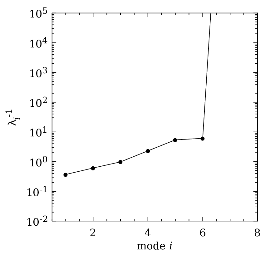
Figure 6 shows the inverse of the largest eigenvalues. Beyond the first six, all the eigenvalues are seen to be negligibly small. It is known that the largest eigenvalue corresponds to minimum variance set by the Cramer-Rao bound and vice versa. This implies that the errors in would increase drastically if modes are included. Hence, most of the relevant information is essentially contained in the first six modes with larger eigenvalues. These normalized eigenmodes are shown in the Figure 7. One can see that, all these modes almost tend to vanish for and , as the Fisher matrix is vanishingly small in these regions. The positions of the spikes and troughs in these modes are related to the presence of data points and their amplitudes depend on the corresponding error-bars (smaller the error, larger the amplitude).
The fiducial model adopted in our analysis may be different from the true model which dictates the data. Clearly, the reconstruction would be poor for wide discrepancies between the two. In our analysis, the simulated bias serves as the input. In the absence of many alternative models for large scale HI bias, this serves as a reasonable fiducial model.
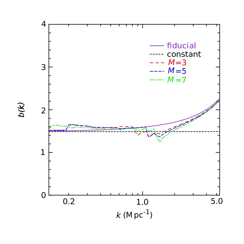
We assume that one can then reconstruct the function using only the first modes (see Eq. 6). Considering all the modes ensures that no information is thrown away. However this is achieved at the cost that errors in the recovered quantities would be very large owing to the presence of the negligibly small eigenvalues. On the contrary, lowering the number of modes can reduce the error but may introduce large biases in the recovered quantities. An important step in this analysis is therefore, to decide on the number of modes to be used. In order to test this we consider a constant bias model to represent the true model as against the fiducial model. For a given data, figure 8 shows how the true model is reconstructed through the inclusion of more and more PCA modes. The reconstruction is directly related to the quality of the data. In the -range where data is not available, the reconstruction is poor and the fiducial model is followed. The reconstruction is also poor for large departures of the true model from the fiducial model. We see that a resonable reconstruction is obtained using the first modes for where the data is available.

In order to fix the value of , we have used the Akaike information criterion [Liddle (2007] , whose smaller values are assumed to imply a more favored model. Following the strategy used by ?) and ?), we have used different values of (2 to 6) for which the AIC is close to its minimum and amalgamated them equally at the Monte Carlo stage when we compute the errors. In this way, we ensure that the inherent bias which exists in any particular choice of is reduced.
We next perform the Monte-Carlo Markov Chain (MCMC) analysis over the parameter space of the optimum number of PCA amplitudes and . Other cosmological parameters are held fixed to the WMAP7 best-fit values (see Section 2). We carry out the analysis by taking to for which the AIC criterion is satisfied. By equal choice of weights for and folding the corresponding errors together we reconstruct and thereby along with their effective errors. We have developed a code based on the publicly available COSMOMC [Lewis & Bridle (2002] for this purpose. A number of distinct chains are run until the Gelman and Rubin convergence statistics satisfies . We have also used the convergence diagnostic of Raftery & Lewis to choose suitable thinning conditions for each chain to obtain statistically independent samples.
5 Results and Discussion


The reconstructed bias function obtained using the analysis described in the last section is shown in Figure 9. The solid line represents the mean model while the shaded region corresponds to 95% confidence limits (2-). We have also shown the fiducial model (short-dashed) as well as the popularly used constant bias, model (long-dashed) for comparison. We find that the fiducial model is within the 95% confidence limits for the entire range considered, while the constant bias is within the same confidence limits only up to . We note that the errors decrease drastically for and . This is expected from the nature of the Fisher matrix which shows that there is practically no information in the PCA modes from these regions. Therefore, all models show a tendency to converge towards the fiducial one. This is a direct manifestation of lack of data points probing these scales. Thus, most of the information is concentrated in the range within which reconstruction of the bias function is relevant with the given data set.
The mean reconstructed bias simply follows the fiducial model for . This is expected as the simulated data is generated using the fiducial bias model itself (Section 3). In the case of analysis using real observed data this matching would have statistical significance, whereas here this just serves as an internal consistency check. The shaded region depicting the errors around the mean is however meaningful and tells us how well the given data can constrain the bias. The outline of the 2- confidence limits shows a jagged feature which is directly related to the presence of the data points. We observe that apart from the fiducial model, a constant bias model is also consistent with the data within the 2- limits. In fact, other than imposing rough bounds , the present data can hardly constrain the scale-dependence of bias. It is also not possible for the data with its error-bars to statistically distinguish between the fiducial and the constant bias model in . Figure 10 illustrates the recovered angular power spectrum with its 95% confidence limits. Superposed on it are the original data points with error-bars. We also show the angular power spectrum calculated for the fiducial and the constant bias models. The 2- contour follows the pattern of the error-bars on the data points. It is evident that the data is largely insensitive (within its error-bars) to the different bias models. Hence the dependence of bias on these scales does not affect the observable quantity within the bounds of statistical precision.
| Parameters | 2- errors |
|---|---|
While constructing the Fisher matrix, we had marginalized over the largely unknown parameter . Treating it as an independent free parameter, we have investigated the possibility of constraining the neutral fraction using the simulated data. The 2- error in this parameter obtained from our analysis is shown in Table 2. We had used the fiducial value in calculating . It is not surprising that our analysis gives a mean which is in excellent agreement with the fiducial value. It is however more important to note that the given data actually constrains reasonable well at .
Noting that, on large scales ( ), one cannot distinguish between the mean, fiducial and the constant bias models, we use to denote the bias value on these scales. The 2- error on is evaluated at (shown in Table 2).
In the range of our interest, the fiducial model does not reflect significant departure from the constant bias. Further, the confidence interval obtained from the data also reflects that the observed is insensitive to the form of bias function in this range - provided that it is bound between approximate cut-offs (). Moreover, the bias largely affects the amplitude of the angular power spectrum and has only a weak contribution towards determining its shape. A scale independent large-scale bias seems to be sufficient in modelling the data. The mean neutral fraction which globally sets the amplitude of the power spectrum is hence weakly degenerate with the bias. This is manifested in the fact that though is rather well constrained, the bias reconstruction which uses the degraded Fisher information (after marginalizing over ) is only weakly constrained from the same data. A prior independent knowledge about the post reionization neutral fraction would clearly ensure a more statistically significant bias reconstruction with smaller errors.
Figure 11 shows the reconstructed 3D HI power spectrum. The direct algebraic relationship between the observable and the bias makes the 3D analysis relatively straightforward. This is specifically evident since the Fisher matrix elements in this case are non-zero only along the diagonal at specific values corresponding to the data points. The entire routine repeated here yields similar generic features. However, the key difference is that we have a larger number of bins with high sensitivity leading to an improved constraining of bias in the range .
In the absence of real observed data, our proposed method applied on a simulated data set, reflects the possibility of constraining large-scale bias. The method is expected to yield better results if one has precise knowledge about the neutral content of the IGM and the underlying cosmological paradigm. We note that the problem of constraining an unknown function given a known data dealt in this work is fairly general and several alternative methods maybe used. The chief advantage of the method adopted here, apart from its effective data reduction, is its model independence. The non-parametric nature of the analysis is specially useful in the absence of any specific prior information. A straightforward fitting of a polynomial and estimating the coeffecients may turn out to be effective but there is no a priori reason to believe that it would work. It is logically more reasonable not to impose a model (with its parameters) upon the data, and instead, let the data reconstruct the model.
With the anticipation of upcoming radio observations towards measurement of power spectrum, our method holds the promise for pinning down the nature of bias thereby throwing valuable light on our understanding of the distribution in the diffuse IGM.
Acknowledgements
Computational work for this study was carried out at the Centre for Theoretical Studies, IIT, Kharagpur and the cluster computing facility of Harish-Chandra Research Institute44 4 http://cluster.hri.res.in/index.html. Suman Majumdar would like acknowledge Council of Scientific and Industrial Research (CSIR), India for providing financial assistance through a Senior Research Fellowship (File No. 9/81(1099)/10-EMR-I). The authors would like to thank Prof. Somnath Bharadwaj for useful discussions and help.
References
- Ali, Bharadwaj & Chengalur (2008 Ali S. S., Bharadwaj S., Chengalur J. N., 2008, MNRAS, 385, 2166
- Bagla, Khandai & Datta (2010 Bagla J. S., Khandai N., Datta K. K., 2010, MNRAS, 407, 567
- Becker, Fan & White (2001 Becker R. H., Fan X., White R. L. e. a., 2001, ApJ, 122, 2850
- Bharadwaj & Ali (2004 Bharadwaj S., Ali S. S., 2004, MNRAS, 352, 142
- Bharadwaj & Ali (2005 Bharadwaj S., Ali S. S., 2005, MNRAS, 356, 1519
- Bharadwaj, Nath & Sethi (2001 Bharadwaj S., Nath B. B., Sethi S. K., 2001, Journal of Astrophysics and Astronomy, 22, 21
- Bharadwaj & Sethi (2001 Bharadwaj S., Sethi S. K., 2001, Journal of Astrophysics and Astronomy, 22, 293
- Bharadwaj, Sethi & Saini (2009 Bharadwaj S., Sethi S. K., Saini T. D., 2009, PRD, 79, 083538
- Bharadwaj & Srikant (2004 Bharadwaj S., Srikant P. S., 2004, Journal of Astrophysics and Astronomy, 25, 67
- Chang et al. (2008 Chang T., Pen U., Peterson J. B., McDonald P., 2008, Physical Review Letters, 100, 091303
- Clarkson & Zunckel (2010 Clarkson C., Zunckel C., 2010, Physical Review Letters, 104, 211301
- Datta, Choudhury & Bharadwaj (2007 Datta K. K., Choudhury T. R., Bharadwaj S., 2007, MNRAS, 378, 119
- Davis et al. (1985 Davis M., Efstathiou G., Frenk C. S., White S. D. M., 1985, ApJ, 292, 371
- Dekel & Lahav (1999 Dekel A., Lahav O., 1999, ApJ, 520, 24
- Efstathiou & Bond (1999 Efstathiou G., Bond J. R., 1999, MNRAS, 304, 75
- Eisenstein & Hu (1998 Eisenstein D. J., Hu W., 1998, ApJ, 496, 605
- Fan, Carilli & Keating (2006 Fan X., Carilli C. L., Keating B., 2006, Annual Review of Astronomy & Astrophysics, 44, 415
- Fang et al. (1993 Fang L., Bi H., Xiang S., Boerner G., 1993, ApJ, 413, 477
- Furlanetto, Oh & Briggs (2006 Furlanetto S. R., Oh S. P., Briggs F. H., 2006, Physics Report, 433, 181
- Ghosh et al. (2010 Ghosh A., Bharadwaj S., Ali S. S., Chengalur J. N., 2010, ArXiv e-prints
- Ghosh et al. (2011 Ghosh A., Bharadwaj S., Saiyad Ali S., Chengalur J. N., 2011, ArXiv e-prints
- Guha Sarkar (2010 Guha Sarkar T., 2010, Journal of Cosmology and Astro-Particle Physics, 2, 2
- Guha Sarkar et al. (2011 Guha Sarkar T., Bharadwaj S., Choudhury T. R., Datta K. K., 2011, MNRAS, 410, 1130
- Guha Sarkar, Datta & Bharadwaj (2009 Guha Sarkar T., Datta K. K., Bharadwaj S., 2009, Journal of Cosmology and Astro-Particle Physics, 8, 19
- Gunn & Peterson (1965 Gunn J. E., Peterson B. A., 1965, ApJ, 142, 1633
- Haehnelt, Steinmetz & Rauch (2000 Haehnelt M. G., Steinmetz M., Rauch M., 2000, ApJ, 534, 594
- Harrison (1970 Harrison E. R., 1970, PRD, 1, 2726
- Hu & Holder (2003 Hu W., Holder G. P., 2003, PRD, 68, 023001
- Jarosik & et al. (2011 Jarosik N., et al. 2011, The Astrophysical Journal Supplement, 192, 14
- Jenkins et al. (2001 Jenkins A., Frenk C. S., White S. D. M., Colberg J. M., Cole S., Evrard A. E., Couchman H. M. P., Yoshida N., 2001, MNRAS, 321, 372
- Komatsu & et al. (2011 Komatsu E., et al. 2011, The Astrophysical Journal Supplement, 192, 18
- Lanzetta, Wolfe & Turnshek (1995 Lanzetta K. M., Wolfe A. M., Turnshek D. A., 1995, ApJ, 440, 435
- Leach (2006 Leach S., 2006, MNRAS, 372, 646
- Lewis & Bridle (2002 Lewis A., Bridle S., 2002, PRD, 66, 103511
- Liddle (2007 Liddle A. R., 2007, MNRAS, 377, L74
- Loeb & Wyithe (2008 Loeb A., Wyithe J. S. B., 2008, Physical Review Letters, 100, 161301
- Loeb & Zaldarriaga (2004 Loeb A., Zaldarriaga M., 2004, Physical Review Letters, 92, 2
- Madau, Meiksin & Rees (1997 Madau P., Meiksin A., Rees M. J., 1997, ApJ, 475, 429
- Mao et al. (2008 Mao Y., Tegmark M., McQuinn M., Zaldarriaga M., Zahn O., 2008, PRD, 78, 023529
- Marín et al. (2010 Marín F. A., Gnedin N. Y., Seo H.-J., Vallinotto A., 2010, ApJ, 718, 972
- McQuinn et al. (2006 McQuinn M., Zahn O., Zaldarriaga M., Hernquist L., Furlanetto S. R., 2006, ApJ, 653, 815
- Mitra, Choudhury & Ferrara (2012 Mitra S., Choudhury T. R., Ferrara A., 2012, MNRAS, 419, 1480
- Mitra, Choudhury & Ferrara (2011 Mitra S., Choudhury T. R., Ferrara A., 2011, MNRAS, 413, 1569
- Mo & White (1996 Mo H. J., White S. D. M., 1996, MNRAS, 282, 347
- Péroux et al. (2003 Péroux C., McMahon R. G., Storrie-Lombardi L. J., Irwin M. J., 2003, MNRAS, 346, 1103
- Pontzen et al. (2008 Pontzen A., Governato F., Pettini M., Booth C. M., Stinson G., Wadsley J., Brooks A., Quinn T., Haehnelt M., 2008, MNRAS, 390, 1349
- Purcell & Field (1956 Purcell E. M., Field G. B., 1956, ApJ, 124, 542
- Rao & Turnshek (2000 Rao S. M., Turnshek D. A., 2000, The Astrophysical Journal Supplement, 130, 1
- Saini, Bharadwaj & Sethi (2001 Saini T. D., Bharadwaj S., Sethi S. K., 2001, ApJ, 557, 421
- Santos, Cooray & Knox (2005 Santos M. G., Cooray A., Knox L., 2005, ApJ, 625, 575
- Sheth & Tormen (2002 Sheth R. K., Tormen G., 2002, MNRAS, 329, 61
- Storrie-Lombardi, McMahon & Irwin (1996 Storrie-Lombardi L. J., McMahon R. G., Irwin M. J., 1996, MNRAS, 283, L79
- Visbal, Loeb & Wyithe (2009 Visbal E., Loeb A., Wyithe S., 2009, Journal of Cosmology and Astro-Particle Physics, 10, 30
- Wolfe, Gawiser & Prochaska (2005 Wolfe A. M., Gawiser E., Prochaska J. X., 2005, Annual Review of Astronomy & Astrophysics, 43, 861
- Wouthuysen (1952 Wouthuysen S. A., 1952, ApJ, 57, 31
- Wyithe & Brown (2009 Wyithe S., Brown M. J. I., 2009, ArXiv e-prints
- Wyithe & Loeb (2007 Wyithe S., Loeb A., 2007, ArXiv e-prints
- Wyithe & Loeb (2008 Wyithe S., Loeb A., 2008, ArXiv e-prints
- Wyithe, Loeb & Geil (2007 Wyithe S., Loeb A., Geil P., 2007, ArXiv e-prints
- Zeldovich (1972 Zeldovich Y. B., 1972, MNRAS, 160, 1P