Detecting Spurious Counterexamples Efficiently in Abstract Model Checking Note: This research is supported by the NSFC Grant No. 61003078, 91018010, 61133001 and 60910004, 973 Program Grant No. 2010CB328102, SRFDP Grant No. 200807010012 and ISN Lab Grant No. ISN1102001.
Abstract
Abstraction is one of the most important strategies for dealing with the state space explosion problem in model checking. In the abstract model, the state space is largely reduced, however, a counterexample found in such a model may not be a real counterexample in the concrete model. Accordingly, the abstract model needs to be further refined. How to check whether or not a reported counterexample is spurious is a key problem in the abstraction-refinement loop. In this paper, a formal definition for spurious path is given. Based on it, efficient algorithms for detecting spurious counterexamples are proposed.
Keywords:
model checking, formal verification, abstraction, refinement, algorithm.1 Introduction
Model checking is an important approach for the verification of hardware, software, multi-agent systems, communication protocols, embedded systems and so forth. The term model checking was coined by Clarke and Emerson [1], as well as Sifakis and Queille [2], independently. The earlier model checking algorithms explicitly enumerated the reachable states of the system in order to check the correctness of a given specification. This restricted the capacity of model checkers to systems with a few million states. Since the number of states can grow exponentially in the number of variables, early implementations were only able to handle small designs and did not scale to examples with industrial complexity. To combat this, kinds of methods, such as abstraction, partial order reduction, OBDD, symmetry and bound technique are applied to model checking to reduce the state space for efficient verification. Thanks to these efforts, model checking has been one of the most successful verification approaches which is widely adopted in industrial community.
Among the techniques for reducing the state space, abstraction is certainly the most important one. Abstraction technique preserves all the behaviors of the concrete system but may introduce behaviors that are not present originally. Thus, if a property (i.e. a temporal logic formula) is satisfied in the abstract model, it will still be satisfied in the concrete model. However, if a property is unsatisfiable in the abstract model, it may still be satisfied in the concrete model, and none of the behaviors that violate the property in the abstract model can be reproduced in the concrete model. In this case, the counterexample is said to be spurious. Thus, when a spurious counterexample is found, the abstraction should be refined in order to eliminate the spurious behaviors. This process is repeated until either a real counterexample is found or the abstract model satisfies the property.
In the abstraction-refinement loop, how to check whether or not a reported counterexample is spurious is a key problem. In [3], algorithm SplitPath is presented for checking whether or not a counterexample is spurious, and a SAT solver is employed to implement it [4, 10]. In SplitPath, whether or not a counterexample is spurious can be checked by detecting the first failure state in the counterexample. If a failure state is found, the counterexample is spurious, otherwise, the counterexample is a real one. However, whether or not a state, say , is a failure state relies on the prefix of the counterexample . This brings in a polynomial number of unwinding of the loop in an infinite counterexample [3, 15].
In this paper, based on a formal definition of failure states, spurious paths are re-analyzed, and a new approach for checking spurious counterexamples is proposed. Within this approach, whether or not a counterexample is spurious still depends on the existence of failure states in the counterexample. Instead of the prefix, to checking whether or not a state is a failure state is only up to ’s pre- and post- states in the counterexample. Based on this, for an infinite counterexample, the polynomial number of unwinding of the loop can be avoided. Further, the algorithm can be easily improved by detecting the heaviest failure state such that a number of model checking iterations can be saved in the whole abstract-refinement loop. In addition, the algorithm can be naturally parallelled.
The rest parts of the paper are organized as follows. The next section briefly presents the preliminaries in abstraction-refinement. In section 3, why spurious counterexamples occur is analyzed intuitively and algorithm SplitPath is briefly presented. In section 4, a formal definition of spurious counterexamples is given with respect to the formal definition of failure states. Further, in section 5, efficient algorithms for checking whether or not a counterexample in the abstract model is spurious are presented. Finally, conclusions are drawn in section 6.
2 Abstraction and Refinement
There are many techniques for obtaining the abstract models [6, 8, 12]. We follow the counterexample guided abstraction and refinement method proposed by Clarke, etc, where abstraction is performed by selecting a set of variables which are insensitive to the desired property to be invisible [4]. We use to denote an abstract function, where is the set of all states in the original model, and the set of all states in the abstract model. For clearance, , , , … are usually used to denote the states in the original model, and , , , … indicate the states in the abstract model. Further, for a state in the abstract model, is used to denote the set of origins of in the original model.
The abstraction-refinement loop is depicted in Fig.1.

Initially, the abstract model is obtained by the abstract function . Then a model checker is employed to check whether or not the abstract model satisfies the desired property. If no errors are found, the model is correct. Otherwise, a counterexample is reported and rechecked by a checker which is used to check whether or not a counterexample is spurious. If the counterexample is not spurious, it will be a real counterexample that violates the system; otherwise, the counterexample is spurious, and a refining tool is used to refine the abstract model [3, 4, 5, 7, 9, 13]. Subsequently, the refined abstract model is checked with the model checker again until either a real counterexample is found or the model is checked to be correct. In this paper, we concentrate on the how to check whether or not a counterexample is spurious.
3 Spurious Paths
To check a spurious counterexample efficiently, we first show why spurious paths occur intuitively with an example. Then we briefly present the basic idea of algorithm SplitPath which is used in [3, 15] for checking whether or not a counterexample is spurious.
3.1 Why Spurious Paths?
Abstraction technique preserves all the behaviors of the concrete system but may introduce behaviors that are not present originally. Therefore, when implementing the model checker with the abstract model, some reported counterexamples will not be real counterexamples that violate the desired property. This is intuitively illustrated by the traffic lights controller example [3].
Example 1
For the traffic light controller in Fig. 2 (1), by making variable color invisible, an abstract model can be obtained as shown in Fig. 2 (2). We want to prove (any time, the state of the light will be sometimes in the future). By implementing model checking with the abstract model,

a counterexample, will be reported. However, in the concrete model, such a behavior cannot be found. So, this is not a real counterexample.
3.2 Detecting Spurious Counterexample with SplitPath
In [3], algorithms SplitPath is presented for checking whether or not a finite counterexample is spurious. In SplitPath, as illustrated in Fig.3, initially, the set, , of starting states falling into ,
is computed. Then for the image of the states in , i.e. , the set of states falling into ,
is computed. Generally, for any ,
is computed recursively. For some state , , if , is a failure state. Note that if , is a failure state. To check whether or not a finite counterexample is spurious, , , , … are computed in turn until the first state where is found, or the last state in the counterexample is reached.
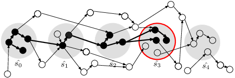
For infinite counterexamples, it is more complicated to be dealt with since the last state in the counterexample can never be reached. Thus, a polynomial number of unwinding of the loop in the counterexample is needed [3]. That is an infinite counterexample can be reduced to a finite counterexample by unwinding the loop for a polynomial number of times. Accordingly, SplitPath can be used again to check whether or not this infinite counterexample is spurious.
4 Failure States and Spurious Counterexamples
In [4, 5], a spurious counterexample is informally defined by: a counterexample in the abstract model which does not exist in the concrete model. In this section, we give a formal definition for spurious counterexamples based on the the formal definition of failure states.
To this end, , , …, and are defined first:
Clearly, denotes the set of states in with inputting edges from the states in , and stands for the set of states in with inputting edges from the states in , and means the set of states in with inputting edges from the states in , and so on. Thus, denotes the set of states in that are reachable from some state in as illustrated in the lower gray part in Fig. 4. Note that there must exist a natural number , such that since is finite. Note that for state ,
That is only is defined differently since there are no pre states.

Similarly, , , …, and can also be defined.
Where denotes the set of states in with outputting edges to the states in , and stands for the set of states in with outputting edges to the states in , and means the set of states in with outputting edges to the states in , and so on. Thus, denotes the set of states in from which some state in are reachable as depicted in the higher gray part in Fig. 4. Similar to , there must exist a natural number , such that . Note that for the last state in a finite counterexample,
where is the set of states without any successors in the original model.
Accordingly, a failure state can be defined as follows.
Definition 1
(Failure States) A state in a counterexample is a failure state if, and only if .
Further, given a failure state in a counterexample , the set of the origins of , , is separated into three sets, (the set of dead states), (the set of bad states) and (the set of the isolated states).
Definition 2
(Spurious Counterexamples) A counterexample in an abstract model is spurious if there exists at least one failure state in
Example 2
Fig. 5 shows a spurious counterexample where state is a failure state.
In the set, , of the origins of state , is a dead state, is a bad state, and is an isolated state.

5 Algorithms for Detecting Spurious Counterexamples
Based on the formal definition of spurious counterexample, new algorithms for checking whether or not a counterexample is spurious are presented in this section.
5.1 Algorithm by Detecting the First Failure State
Algorithm CheckSpurious-I takes a counterexample as input and outputs the first failure state in the counterexample. Note that a counterexample may be a finite path , , or an infinite path , , with a loop suffix (a suffix produced by a loop). For the finite one, it can be checked directly; while for an infinite one, we need only to check its Complete Finite Prefix (CFP) since whether or not a state is a failure state only relies on its pre and post states. It is pointed out that in the CFP of an infinite counterexample,
since the post state of is .
Input: a counterexample in the abstract model , and the original model
Output: a failure state
Algorithm Analyzing
In algorithm CheckSpurious-I, to check whether or not a state is a failure state only relies on ’s pre and post states, and ; while in algorithm SplitPath, to check state is up to the prefix, , of . Based on this, to check a periodic infinite counterexample, several repetitions of the periodic parts are needed in SplitPath. In contrast, this can be easily done by checking the complete finite prefix in algorithm CheckSpurious-I. Thus, the polynomial number of unwinding of the loop can be avoided. That is for infinite counterexamples, the finite prefix to be checked will be polynomial shorter than the one in algorithm SplitPath.
5.2 Algorithm by Detecting the Heaviest Failure State
In algorithm SplitPath and CheckSpurious-I, always, the first failure state is detected. Then further refinement will be done based on the analysis of this failure state.
Input: a counterexample in the abstract model , and the original model
Output: the heaviest failure state
Possibly, several failure states may occur in one counterexample, so which one is chosen to be refined is not considered in SplitPath. Obviously, if a failure state shared by more paths is refined, a number of model checking iterations will be saved in the whole abstract-refinement loop. With this consideration, we will check the states which is shared by more paths first. To do so, for an abstract state as illustrated in Fig.6,

and are defined. equals to the number of edges connecting to the states in from the states outside of ; and is the number of edges connecting to the states out of from the states in . Accordingly, is the number of the paths where occurs. For convenience, we call the weight of the abstract state . Based on this, algorithm CheckSpurious-II is given for detecting the heaviest failure state in a counterexample. In CheckSpurious-II, an array w[i] is used to store the indexes of the states in the counterexample by the heavier the earlier.
5.3 Parallel Algorithms
Considering whether or not a state is a failure state only relies on the pre- and post- states, and , of , the algorithm can be naturally paralleled as presented in algorithm CheckSpurious-III and CheckSpurious-IV.
In CheckSpurious-III, anytime, if a failure state is detected by a processor, all the processors will be stop and the failure state is returned. Otherwise, if no failure states are reported, the counterexample is a real one. That is the algorithm always reports the first detected failure state obtained by the processors. Note that a boolean array is used to indicate whether or not a state in the counterexample is a failure one. Initially, for all , is undefined (). means state is not a failure state.
Input: a counterexample in the abstract model , and the original model in shared memory
: the number of processors
: processor id
Output: a failure state
In CheckSpurious-IV, the weight of the states are considered, and always the heaviest failure state is found.
Input: a counterexample in the abstract model , and the original model in shared memory
: the number of processors
: processor id
Output: a failure state
6 Conclusion
Based on a formal definition of spurious paths, a novel approach for detecting spurious counterexamples are presented in this paper. In the new approach, whether or not a state is a failure state only relies on ’s pre- and post- states in the counterexample. So, for infinite counterexample, the polynomial number of unwinding of the loop can be avoided. Further, the algorithm can be easily improved by detecting the heaviest failure state such that a number of model checking iterations can be saved in the whole abstract-refinement loop. Also, the algorithm can be naturally parallelled.
The presented algorithms are useful in improving the abstract based model checking, especially the counterexample guided abstraction refinement model checking. In the near future, the proposed algorithm will be implemented and integrated into the tool CEGAR. Further, some case studies will be conducted to evaluate the algorithms.
References
- [1] E.M.Clarke and E.A.Emerson. Desigh and syntesis of of synchronization skeletons using branching time temporal logic. In Logic of Programs: Workshop, Yorktown Heights, NY, May 1981, LNCS 131, Springer, 1981.
- [2] J.P.Quielle and J.Sifakis. Specification and verification of concurrent systems in CESAR. In Proceedings of the 5th international symposium on programming, pp.337-350, 1981.
- [3] E.Clarke, O.Grumberg, S.Jha, Y.Lu, and H.Veith. Counterexample guided abstraction refinement, in Proc. 12th Int. Conf. Computer-Aided Verification (CAV¡¯00), vol. 1855, E. Emerson and A. Sistla, Eds. New York, 2000.
- [4] Clarke, E.M., Gupta, A., Strichman, O. SAT Based Counterexample-Guided Abstraction-Refinement. IEEE Trans. Computer Aided Design, vol.23, no. 7, pp. 1113-1123, July 2004.
- [5] Fei He, Xiaoyu Song, William N. N. Hung, Ming Gu, Jiaguang Sun. Integrating Evolutionary Computation with Abstraction Refinement for Model Checking. IEEE Trans. Computers 59(1): 116-126 (2010)
- [6] J. Rushby. Integrated formal verification: Using model checking with automated abstraction, invariant generation, and theorem proving. presented at Theoretical and Practical Aspects of SPIN Model Checking: Proc. 5th and 6th Int. SPIN Workshops. [Online]. Available: citeseer.nj.nec.com/rushby99integrated.html
- [7] Fei He, Xiaoyu Song, William N. N. Hung, Ming Gu, Jiaguang Sun. Integrating Evolutionary Computation with Abstraction Refinement for Model Checking. IEEE Trans. Computers 59(1): 116-126 (2010)
- [8] R.P.Kurshan. Computer Aided Verificaton of Coordinating Processes. Princeton Univ. Press, 1994.
- [9] C. Wang, B. Li, H. Jin, G.D. Hachtel, F. Somenzi. Improving Ariadne’s Bundle by Following Multiple Threads in Abstraction Refinement. IEEE Trans. Computer Aided Design, vol. 25, no. 11, pp. 2297-2316, Nov. 2006.
- [10] E.M. Clarke, A. Gupta, J.H. Kukula, and O. Strichman. SAT Based Abstraction-Refinement Using ILP and Machine Learning Techniques. Proc. Computer-Aided Verification (CAV), E. Brinksma and K.G. Larsen, eds., pp. 265-279, 2002.
- [11] P. Chauhan, E.M. Clarke, J. Kukula, S. Sapra, H. Veith, and D. Wang. Automated Abstraction Refinement for Model Checking Large State Spaces Using SAT Based Conflict Analysis. Proc. Formal Methods in Computer-Aided Design (FMCAD), 2002.
- [12] T.A. Henzinger, R. Jhala, R. Majumdar, and G. Sutre. Lazy Abstraction. Proc. Symp. Principles of Programming Languages, pp. 58-70, 2002.
- [13] M. Glusman, G. Kamhi, S. Mador-Haim, R. Fraer, M.Y. Vardi. Multiple-Counterexample Guided Iterative Abstraction Refinement: An Industrial Evaluation. Proc. Tools and Algorithms for the Construction and Analysis of Systems (TACAS), pp. 176-191, 2003.
- [14] S.G. Govindaraju, D.L. Dill. Counterexample-Guided Choice of Projections in Approximate Symbolic Model Checking. Proc. Int¡¯l Conf. Computer-Aided Design (ICCAD), pp. 115-119, 2000.
- [15] E. Clarke, O. Grumberg, S. Jha, Y. Lu, and H. Veith. Counterexample-guided abstraction refinement. Technical Report CMU-CS-00-103, Computer Science, Carnegie Mellon University, 2000.