Shannon Meets Nyquist:
Capacity of Sampled Gaussian Channels

Yuxin Chen Yonina C. Eldar Andrea J. Goldsmith ^†^†thanks: Y. Chen is with the Department of Electrical Engineering and the Department of Statistics, Stanford University, Stanford, CA 94305, USA (email: yxchen@stanford.edu). Y. C. Eldar is with the Department of Electrical Engineering, Technion, Israel Institute of Technology Haifa, Israel 32000, and has been a visiting professor at Stanford University (email: yonina@ee.technion.ac.il). A. J. Goldsmith is with the Department of Electrical Engineering, Stanford University, Stanford, CA 94305, USA (email: andrea@wsl.stanford.edu). The contact author is Y. Chen. This work was supported in part by the NSF Center for Science of Information, the Interconnect Focus Center of the Semiconductor Research Corporation, and BSF Transformative Science Grant 2010505. It was presented in part at the IEEE International Conference on Acoustics, Speech and Signal Processing (ICASSP) 2011, the 49 Annual Allerton Conference on Communication, Control, and Computing, and IEEE Information Theory Workshop 2011. Copyright (c) 2012 IEEE. Personal use of this material is permitted. However, permission to use this material for any other purposes must be obtained from the IEEE by sending a request to pubs-permissions@ieee.org.

Abstract

We explore two fundamental questions at the intersection of sampling theory and information theory: how channel capacity is affected by sampling below the channel’s Nyquist rate, and what sub-Nyquist sampling strategy should be employed to maximize capacity. In particular, we derive the capacity of sampled analog channels for three prevalent sampling strategies: sampling with filtering, sampling with filter banks, and sampling with modulation and filter banks. These sampling mechanisms subsume most nonuniform sampling techniques applied in practice. Our analyses illuminate interesting connections between under-sampled channels and multiple-input multiple-output channels. The optimal sampling structures are shown to extract out the frequencies with the highest SNR from each aliased frequency set, while suppressing aliasing and out-of-band noise. We also highlight connections between undersampled channel capacity and minimum mean-squared error (MSE) estimation from sampled data. In particular, we show that the filters maximizing capacity and the ones minimizing MSE are equivalent under both filtering and filter-bank sampling strategies. These results demonstrate the effect upon channel capacity of sub-Nyquist sampling techniques, and characterize the tradeoff between information rate and sampling rate.

Index Terms:

sampling rate, channel capacity, sampled analog channels, sub-Nyquist sampling

I Introduction

The capacity of continuous-time Gaussian channels and the corresponding capacity-achieving water-filling power allocation strategy over frequency are well-known [1], and provide much insight and performance targets for practical communication system design. These results implicitly assume sampling above the Nyquist rate at the receiver end. However, channels that are not bandlimited have an infinite Nyquist rate and hence cannot be sampled at that rate. Moreover, hardware and power limitations often preclude sampling at the Nyquist rate associated with the channel bandwidth, especially for wideband communication systems. This gives rise to several natural questions at the intersection of sampling theory and information theory, which we will explore in this paper: (1) how much information, in the Shannon sense, can be conveyed through undersampled analog channels; (2) under a sub-Nyquist sampling-rate constraint, which sampling structures should be chosen in order to maximize information rate.

I-A Related Work

The derivation of the capacity of linear time-invariant (LTI) channels was pioneered by Shannon [2]. Making use of the asymptotic spectral properties of Toeplitz operators [3], this capacity result established the optimality of a water-filling power allocation based on signal-to-noise ratio (SNR) across the frequency domain [1]. Similar results for discrete-time Gaussian channels have also been derived using Fourier analysis [4]. On the other hand, the Shannon-Nyquist sampling theorem, which dictates that channel capacity is preserved when the received signal is sampled at or above the Nyquist rate, has frequently been used to transform analog channels into their discrete counterparts (e.g.[5, 6]). For instance, this paradigm of discretization was employed by Medard to bound the maximum mutual information in time-varying channels [7]. However, all of these works focus on analog channel capacity sampled at or above the Nyquist rate, and do not account for the effect upon capacity of reduced-rate sampling.

The Nyquist rate is the sampling rate required for perfect reconstruction of bandlimited analog signals or, more generally, the class of signals lying in shift-invariant subspaces. Various sampling methods at this sampling rate for bandlimited functions have been proposed. One example is recurrent non-uniform sampling proposed by Yen [8], which samples the signal in such a way that all sample points are divided into blocks where each block contains $N$ points and has a recurrent period. Another example is generalized multi-branch sampling first analyzed by Papoulis [9], in which the input is sampled through $M$ linear systems. For perfect recovery, these methods require sampling at an aggregate rate above the Nyquist rate.

In practice, however, the Nyquist rate may be excessive for perfect reconstruction of signals that possess certain structures. For example, consider multiband signals, whose spectral content resides continuously within several subbands over a wide spectrum, as might occur in a cognitive radio system. If the spectral support is known a priori, then the sampling rate requirement for perfect recovery is the sum of the subband bandwidths, termed the Landau rate [10]. One type of sampling mechanism that can reconstruct multiband signals sampled at the Landau rate is a filter bank followed by sampling, studied in [11, 12]. The basic sampling paradigm of these works is to apply a bank of prefilters to the input, each followed by a uniform sampler.

When the channel or signal structure is unknown, sub-Nyquist sampling approaches have been recently developed to exploit the structure of various classes of input signals, such as multiband signals [13]. In particular, sampling with modulation and filter banks is very effective for signal reconstruction, where the key step is to scramble spectral contents from different subbands through the modulation operation. Examples includes the modulated wideband converter proposed by Mishali et al. [13, 14]. In fact, modulation and filter-bank sampling represents a very general class of realizable nonuniform sampling techniques applied in practice.

Most of the above sampling theoretic work aims at finding optimal sampling methods that admit perfect recovery of a class of analog signals from noiseless samples. There has also been work on minimum reconstruction error from noisy samples based on certain statistical measures (e.g. mean squared error (MSE)). Another line of work pioneered by Berger et. al. [15, 16, 17, 18] investigated joint optimization of the transmitted pulse shape and receiver prefiltering in pulse amplitude modulation over a sub-sampled analog channel. In this work the optimal receiver prefilter that minimizes the MSE between the original signal and the reconstructed signal is shown to prevent aliasing. However, this work does not consider optimal sampling techniques based on capacity as a metric. The optimal filters derived in [15, 16] are used to determine an SNR metric which in turn is used to approximate sampled channel capacity based on the formula for capacity of bandlimited AWGN channels. However, this approximation does not correspond to the precise channel capacity we derive herein, nor is the capacity of more general undersampled analog channels considered.

The tradeoff between capacity and hardware complexity has been studied in another line of work on sampling precision [19, 20]. These works demonstrate that, due to quantization, oversampling can be beneficial in increasing achievable data rates. The focus of these works is on the effect of oversampling upon capacity loss due to quantization error, rather than the effect of quantization-free subsampling upon channel capacity.

I-B Contribution

In this paper, we explore sampled Gaussian channels with the following three classes of sampling mechanisms: (1) a filter followed by sampling: the analog channel output is prefiltered by an LTI filter followed by an ideal uniform sampler (see Fig. 2); (2) filter banks followed by sampling: the analog channel output is passed through a bank of LTI filters, each followed by an ideal uniform sampler (see Fig. 3); (3) modulation and filter banks followed by sampling: the channel output is passed through $M$ branches, where each branch is prefiltered by an LTI filter, modulated by different modulation sequences, passed through another LTI filter and then sampled uniformly. Our main contributions are summarized as follows.

•

Filtering followed by sampling. We derive the sampled channel capacity in the presence of both white and colored noise. Due to aliasing, the sampled channel can be represented as a multiple-input single output (MISO) Gaussian channel in the spectral domain, while the optimal input effectively performs maximum ratio combining. The optimal prefilter is derived and shown to extract out the frequency with the highest SNR while suppressing signals from all other frequencies and hence preventing aliasing. This prefilter also minimizes the MSE between the original signal and the reconstructed signal, illuminating a connection between capacity and MMSE estimation.
•

Filter banks followed by sampling. A closed-form expression for sampled channel capacity is derived, along with analysis that relates it to a multiple-input multiple-output (MIMO) Gaussian channel. We also derive optimal filter banks that maximize capacity. The $M$ filters select the $M$ frequencies with highest SNRs and zero out signals from all other frequencies. This alias-suppressing strategy is also shown to minimize the MSE between the original and reconstructed signals. This mechanism often achieves larger sampled channel capacity than a single filter followed by sampling if the channel is non-monotonic, and it achieves the analog capacity of multiband channels at the Landau rate if the number of branches is appropriately chosen.
•

Modulation and filter banks followed by sampling. For modulation sequences that are periodic with period $T_{q}$ , we derive the sampled channel capacity and show its connection to a general MIMO Gaussian channel in the frequency domain. For sampling following a single branch of modulation and filtering, we provide an algorithm to identify the optimal modulation sequence for piece-wise flat channels when $T_{q}$ is an integer multiple of the sampling period. We also show that the optimal single-branch mechanism is equivalent to an optimal filter bank with each branch sampled at a period $T_{q}$ .

One interesting fact we discover for all these techniques is the non-monotonicity of capacity with sampling rate, which indicates that at certain sampling rates, channel degrees of freedom are lost. Thus, more sophisticated sampling techniques are needed to maximize achievable data rates at sub-Nyquist sampling rates in order to preserve all channel degrees of freedom.

Table I: Summary of Notation and Parameters

$\mathcal{L}_{1}$	set of measurable functions $f$ such that $\int\left\|f\right\|\mathrm{d}\mu<\infty$
$\mathbb{S}_{+}$	set of positive semidefinite matrices
$h(t)$ , $H(f)$	impulse response, and frequency response of the analog channel
$s_{i}(t)$ , $S_{i}(f)$	impulse response, and frequency response of the $i$ th post-modulation filter
$p_{i}(t)$ , $P_{i}(f)$	impulse response, and frequency response of the $i$ th pre-modulation filter
$\mathcal{S}_{\eta}(f)$ , $\mathcal{S}_{x}(f)$	power spectral density of the noise $\eta(t)$ and the stationary input signal $x(t)$
$M$	number of prefilters
$f_{s}$ , $T_{s}$	aggregate sampling rate, and the corresponding sampling interval ( $T_{s}=1/f_{s}$ )
$q_{i}(t)$	modulating sequence in the $i$ th channel
$T_{q}$	period of the modulating sequence $q_{i}(t)$
$\left\\|\cdot\right\\|_{\text{F}}$ , $\left\\|\cdot\right\\|_{2}$	Frobenius norm, $\ell_{2}$ norm
$\left[x\right]^{+}$ , $\log^{+}x$	$\max\left\{x,0\right\}$ , $\max\left\{\log x,0\right\}$

I-C Organization

The remainder of this paper is organized as follows. In Section II, we describe the problem formulation of sampled analog channels. The capacity results for three classes of sampling strategies are presented in Sections III–V. In each section, we analyze and interpret the main theorems based on Fourier analysis and MIMO channel capacity, and identify sampling structures that maximize capacity. The connection between the capacity-maximizing samplers and the MMSE samplers is provided in Section VI. Proofs of the main theorems are provided in the appendices, and the notation is summarized in Table I.

II Preliminaries: Capacity of undersampled channels

II-A Capacity Definition

We consider the continuous-time additive Gaussian channel (see [1, Chapter 8]), where the channel is modeled as an LTI filter with impulse response $h(t)$ and frequency response $H(f)=\int_{-\infty}^{\infty}h(t)\exp(-j2\pi ft)\text{d}t$ . The transmit signal $x(t)$ is time-constrained to the interval $(0,T]$ . The analog channel output is given as

r(t)=h(t)*x(t)+\eta(t),

(1)

and is observed over¹¹ 1 We impose the assumption that both the transmit signal and the observed signal are constrained to finite time intervals to allow for a rigorous definition of channel capacity. In particular, as per Gallager’s analysis [1, Chapter 8], we first calculate the capacity for finite time intervals and then take the limit of the interval to infinity. $\left(0,T\right]$ , where $\eta(t)$ is stationary zero-mean Gaussian noise. We assume throughout the paper that perfect channel state information, i.e. perfect knowledge of $h(t)$ , is known at both the transmitter and the receiver. The analog channel capacity is defined as [1, Section 8.1]

C=\lim_{T\rightarrow\infty}\frac{1}{T}\sup I\left(\left\{x(t)\right\}_{t=0}^{T};\left\{r(t)\right\}_{t=0}^{T}\right),

where the supremum is over all input distributions subject to an average power constraint $\mathbb{E}(\frac{1}{T}\int_{0}^{T}\left|x(\tau)\right|^{2}\mathrm{d}\tau)\leq P$ . Since any given analog channel can be converted to a countable number of independent parallel discrete channels by a Karhunen-Loeve decomposition, the capacity metric quantifies the maximum mutual information between the input and output of these discrete channels. If we denote $[x]^{+}=\max\{x,0\}$ and $\log^{+}x=\max\left\{0,\log x\right\}$ , then the analog channel capacity is given as follows.

Theorem 1.

[1, Theorem 8.5.1] Consider an analog channel with power constraint $P$ and noise power spectral density $\mathcal{S}_{\eta}(f)$ . Assume that $\left|H(f)\right|^{2}/\mathcal{S}_{\eta}(f)$ is bounded and integrable, and that either $\int_{-\infty}^{\infty}\mathcal{S}_{\eta}(f)\mathrm{d}f<\infty$ or that $\mathcal{S}_{\eta}(f)$ is white. Then the analog channel capacity is given by

\displaystyle C

\displaystyle=\frac{1}{2}{\displaystyle\int}_{-\infty}^{\infty}\log^{+}\left(\nu\frac{\left|H\left(f\right)\right|^{2}}{\mathcal{S}_{\eta}(f)}\right)\mathrm{d}f,

(2)

where $\nu$ satisfies

{\displaystyle\int}_{-\infty}^{\infty}\left[\nu-\frac{\mathcal{S}_{\eta}(f)}{\left|H\left(f\right)\right|^{2}}\right]^{+}\mathrm{d}f=P.

(3)

For a channel whose bandwidth lies in $[-B,B]$ , if we remove the noise outside the channel bandwidth via prefiltering and sample the output at a rate $f\geq 2B$ , then we can perfectly recover all information conveyed within the channel bandwidth, which allows (2) to be achieved without sampling loss. For this reason, we will use the terminology Nyquist-rate channel capacity for the analog channel capacity (2), which is commensurate with sampling at or above the Nyquist rate of the received signal after optimized prefiltering.

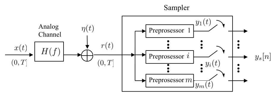
Under sub-Nyquist sampling, the capacity depends on the sampling mechanism and its sampling rate. Specifically, the channel output $r(t)$ is now passed through the receiver’s analog front end, which may include a filter, a bank of $M$ filters, or a bank of preprocessors consisting of filters and modulation modules, yielding a collection of analog outputs $\left\{y_{i}(t):\text{ }1\leq i\leq M\right\}$ . We assume that the analog outputs are observed over the time interval $\left(0,T\right]$ and then passed through ideal uniform samplers, yielding a set of digital sequences $\left\{y_{i}[n]:\text{ }n\in\mathbb{Z},\text{ }1\leq i\leq M\right\}$ , as illustrated in Fig. 1. Here, each branch is uniformly sampled at a sampling rate of $f_{s}/M$ samples per second.

Refer to caption — Figure 1: Sampled Gaussian channel. The input $x(t)$ , constrained to $(0,T]$ , is passed through $M$ branches of the receiver analog front end to yield analog outputs $\left\{y_{i}(t):\text{ }1\leq i\leq M\right\}$ ; each $y_{i}(t)$ is observed over $\left(0,T\right]$ and uniformly sampled at a rate $f_{s}/M$ to yield the sampled sequence $y_{i}[n]$ . The preprocessor can be a filter, or combination of a filter and a modulator.

Define ${\bf y}[n]=\left[y_{1}[n],\cdots,y_{M}[n]\right]$ , and denote by $I(\left\{x(t)\right\}_{t=0}^{T};\left\{{\bf y}[n]\right\}_{t=0}^{T})$ the mutual information between the input $x(t)$ on the interval $0<t\leq T$ and the samples $\left\{y[n]\right\}$ observed on the interval $0<t\leq T$ . We pose the problem of finding the capacity $C(f_{s})$ of sampled channels as quantifying the maximum mutual information in the limit as $T\rightarrow\infty$ . The sampled channel capacity can then be expressed as

C(f_{s})=\lim_{T\rightarrow\infty}\frac{1}{T}\sup I\left(\left\{x(t)\right\}_{t=0}^{T};\left\{{\bf y}[n]\right\}_{t=0}^{T}\right),

where the supremum is over all possible input distributions subject to an average power constraint $\mathbb{E}(\frac{1}{T}\int_{0}^{T}\left|x(\tau)\right|^{2}\mathrm{d}\tau)\leq P$ . We restrict the transmit signal $x(t)$ to be continuous with bounded variance (i.e. $\sup_{t}\mathbb{E}\left|x(t)\right|^{2}<\infty$ ), and restrict the probability measure of $x(t)$ to be uniformly continuous. This restriction simplifies some mathematical analysis, while still encompassing most practical signals of interests ²² 2 Note that this condition is not necessary for our main theorems. An alternative proof based on correlation functions is provided in [21], which does not require this condition..

II-B Sampling Mechanisms

In this subsection, we describe three classes of sampling strategies with increasing complexity. In particular, we start from sampling following a single filter, and extend our results to incorporate filter banks and modulation banks.

II-B1 Filtering followed by sampling

Ideal uniform sampling is performed by sampling the analog signal uniformly at a rate $f_{s}=T_{s}^{-1}$ , where $T_{s}$ denotes the sampling interval. In order to avoid aliasing, suppress out-of-band noise, and compensate for linear distortion of practical sampling devices, a prefilter is often added prior to the ideal uniform sampler [22]. Our sampling process thus includes a general analog prefilter, as illustrated in Fig. 2. Specifically, before sampling, we prefilter the received signal with an LTI filter that has impulse response $s(t)$ and frequency response $S\left(f\right)$ , where we assume that $h(t)$ and $s(t)$ are both bounded and continuous. The filtered output is observed over $(0,T]$ and can be written as

y(t)=s(t)*\left(h(t)*x(t)+\eta(t)\right),\quad t\in\left(0,T\right].

(4)

We then sample $y(t)$ using an ideal uniform sampler, leading to the sampled sequence

y[n]=y(nT_{s}).

Figure 3: A filter bank followed by sampling: the received analog signal

r(t)

is passed through

M

branches. In the

i

th branch, the signal

r(t)

is passed through an LTI prefilter with impulse response

s_{i}(f)

, and then sampled uniformly at a rate

f_{s}/M

II-B2 Sampling following Filter Banks

Sampling following a single filter often falls short of exploiting channel structure. In particular, although Nyquist-rate uniform sampling preserves information for bandlimited signals, for multiband signals it does not ensure perfect reconstruction at the Landau rate (i.e. the total widths of spectral support). That is because uniform sampling at sub-Nyquist rates may suppress information by collapsing subbands, resulting in fewer degrees of freedom. This motivates us to investigate certain nonuniform sampling mechanisms. We begin by considering a popular class of non-uniform sampling mechanisms, where the received signal is preprocessed by a bank of filters. Most practical nonuniform sampling techniques [9, 11, 12] fall under filter-bank sampling and modulation-bank sampling (as described in Section II-B3). Note that the filters may introduce delays, so that this approach subsumes that of a filter bank with different sampling times at each branch.

In this sampling strategy, we replace the single prefilter in Fig. 2 by a bank of $M$ analog filters each followed by ideal sampling at rate $f_{s}/M$ , as illustrated in Fig. 3. We denote by $s_{i}(t)$ and $S_{i}\left(f\right)$ the impulse response and frequency response of the $i$ th LTI filter, respectively. The filtered analog output in the $i$ th branch prior to sampling is then given as

y_{i}(t)=\left(h(t)*s_{i}(t)\right)*x(t)+s_{i}(t)*\eta(t),\quad t\in\left(0,T\right].

(5)

These filtered signals are then sampled uniformly to yield

y_{i}[n]\overset{\Delta}{=}y_{i}(nMT_{s})\quad\text{and}\quad{\bf y}[n]\overset{\Delta}{=}\left[y_{1}[n],y_{2}[n],\cdots,y_{M}[n]\right],

where $T_{s}=f_{s}^{-1}$ .

II-B3 Modulation and Filter Banks Followed by Sampling

We generalize the filter-bank sampling strategy by adding an additional filter bank and a modulation bank, which includes as special cases a broad class of nonuniform sampling methods that are applied in both theory and practice. Specifically, the sampling system with sampling rate $f_{s}$ comprises $M$ branches. In the $i$ th branch, the received signal $r(t)$ is prefiltered by an LTI filter with impulse response $p_{i}(t)$ and frequency response $P_{i}(f)$ , modulated by a periodic waveform $q_{i}(t)$ of period $T_{q}$ , filtered by another LTI filter with impulse response $s_{i}(t)$ and frequency response $S_{i}(f)$ , and then sampled uniformly at a rate $f_{s}/M=\left(MT_{s}\right)^{-1}$ , as illustrated in Fig. 4. The first prefilter $P_{i}(f)$ will be useful in removing out-of-band noise, while the periodic waveforms scramble spectral contents from different aliased sets, thus bringing in more design flexibility that may potentially lead to better exploitation of channel structure. By taking advantage of random modulation sequences to achieve incoherence among different branches, this sampling mechanism has proven useful for sub-sampling multiband signals [13].

Figure 4: Modulation and filter banks followed by sampling: in each branch, the received signal is prefiltered by an LTI filter with impulse response

p_{i}(t)

, modulated by a periodic waveform

q_{i}(t)

, filtered by another LTI filter with impulse response

s_{i}(t)

, and then sampled at a rate

f_{s}/M

In the $i$ th branch, the analog signal after post-modulation filtering prior to sampling can be written as

y_{i}(t)=s_{i}(t)*\left(q_{i}(t)\cdot\left[p_{i}(t)*\left(h(t)*x(t)+\eta(t)\right)\right]\right),

(6)

resulting in the digital sequence of samples

y_{i}[n]=y_{i}(nMT_{s})\quad\text{and}\quad{\bf y}\left[n\right]=\left[y_{1}\left[n\right],\cdots,y_{M}\left[n\right]\right]^{T}.

III A Filter Followed by Sampling

III-A Main Results

The sampled channel capacity under sampling with filtering is stated in the following theorem.

Theorem 2.

Consider the system shown Fig. 2, where $\eta(t)$ is Gaussian noise with power spectral density $\mathcal{S}_{\eta}(f)$ . Assume that $h(t)$ , $s(t)$ , $S\left(f\right)\sqrt{\mathcal{S}_{\eta}\left(f\right)}$ are all continuous, bounded and absolutely Riemann integrable. Additionally, suppose that $h_{\eta}(t):=\mathcal{F}^{-1}\left(\frac{H\left(f\right)}{\sqrt{\mathcal{S}_{\eta}\left(f\right)}}\right)$ satisfies $h_{\eta}(t)=o\left(t^{-\epsilon}\right)$ for some constant ³³ 3 This condition is used in Appendix A as a sufficient condition to guarantee asymptotic properties of Toeplitz matrices. A similar condition will be used in Theorems 4 and 6. $\epsilon>1$ . The capacity $C(f_{s})$ of the sampled channel with a power constraint $P$ is then given parametrically as

\displaystyle C\left(f_{s}\right)

\displaystyle={\displaystyle\int}_{-\frac{f_{s}}{2}}^{\frac{f_{s}}{2}}\frac{1}{2}\log^{+}\left(\nu\gamma^{\text{s}}(f)\right)\mathrm{d}f,

(7)

where $\nu$ satisfies

{\displaystyle\int}_{-\frac{f_{s}}{2}}^{\frac{f_{s}}{2}}\left[\nu-1/\gamma^{\text{s}}(f)\right]^{+}\mathrm{d}f=P.

(8)

Here, we denote

\gamma^{\text{s}}(f):=\frac{\underset{l\in\mathbb{Z}}{\sum}\left|H(f-lf_{s})S(f-lf_{s})\right|^{2}}{\underset{l\in\mathbb{Z}}{\sum}\left|S(f-lf_{s})\right|^{2}\mathcal{S}_{\eta}(f-lf_{s})}.

As expected, applying the prefilter modifies the channel gain and colors the noise accordingly. The color of the noise is reflected in the denominator term of the corresponding SNR in (7) at each $f\in[-f_{s}/2,f_{s}/2]$ within the sampling bandwidth. The channel and prefilter response leads to an equivalent frequency-selective channel, and the ideal uniform sampling that follows generates a folded version of the non-sampled channel capacity. Specifically, this capacity expression differs from the analog capacity given in Theorem 1 in that the SNR in the sampled scenario is $\gamma^{\text{s}}(f)$ in contrast to $\left|H(f)\right|^{2}/\mathcal{S}_{\eta}(f)$ for the non-sampled scenario. Water filling over $1/\gamma^{\text{s}}(f)$ determines the optimal power allocation.

III-B Approximate Analysis

Rather than providing here a rigorous proof of Theorem 2, we first develop an approximate analysis by relating the aliased channel to MISO channels, which allows for a communication theoretic interpretation. The rigorous analysis, which is deferred to Appendix A, makes use of a discretization argument and asymptotic spectral properties of Toeplitz matrices.

Consider first the equivalence between the sampled channel and a MISO channel at a single frequency $f\in[-f_{s}/2,f_{s}/2]$ . As part of the approximation, we suppose the Fourier transform $X(f)$ of the transmitted signal exists⁴⁴ 4 The Fourier transform of the input signal typically does not exist since the input may be a stationary process. . The Fourier transform of the sampled signal at any $f\in[-f_{s}/2,f_{s}/2]$ is given by

\frac{1}{T_{s}}\sum_{k\in\mathbb{Z}}H\left(f-kf_{s}\right)S(f-kf_{s})X\left(f-kf_{s}\right)

(9)

due to aliasing. The summing operation allows us to treat the aliased channel at each $f$ within the sampling bandwidth as a separate MISO channel with countably many input branches and a single output branch, as illustrated in Fig. 5.

By assumption, the noise has spectral density $\mathcal{S}_{\eta}(f)$ , so that the filtered noise has power spectral density $\mathcal{S}_{\eta}(f)|S(f)|^{2}$ . The power spectral density of the sampled noise sequence at $f\in[-f_{s}/2,f_{s}/2]$ is then given by $\sum_{l\in\mathbb{Z}}\mathcal{S}_{\eta}(f-lf_{s})\left|S(f-lf_{s})\right|^{2}$ . If we term $\left\{f-lf_{s}\mid\text{ }l\in\mathbb{Z}\right\}$ the aliased frequency set for $f$ , then the amount of power allocated to $X(f-lf_{s})$ should “match” the corresponding channel gain within each aliased set in order to achieve capacity. Specifically, denote by $G(f)$ the transmitted signal for every $f\in[-f_{s}/2,f_{s}/2]$ . This signal is multiplied by a constant gain $c\alpha_{l}\text{ }(l\in\mathbb{Z})$ , and sent through the $l$ th input branch, i.e.

X\left(f-lf_{s}\right)=c\alpha_{l}G(f),\quad\forall l\in\mathbb{Z},

(10)

where $c$ is a normalizing constant, and

\alpha_{l}=\frac{H^{*}\left(f-lf_{s}\right)S^{*}\left(f-lf_{s}\right)}{\sum_{l}\left|H(f-lf_{s})S(f-lf_{s})\right|^{2}}.

The resulting SNR can be expressed as the sum of SNRs (as shown in [23]) at each branch. Since the sampling operation combines signal components at frequencies from each aliased set $\left\{f-lf_{s}\mid l\in\mathbb{Z}\right\}$ , it is equivalent to having a set of parallel MISO channels, each indexed by some $f\in[-f_{s}/2,f_{s}/2]$ . The water-filling strategy is optimal in allocating power among the set of parallel channels, which yields the parametric equation (8) and completes our approximate analysis.

III-C Proof Sketch

Since the Fourier transform is not well-defined for signals with infinite energy, there exist technical flaws lurking in the approximate treatment of the previous subsection. The key step to circumvent these issues is to explore the asymptotic properties of Toeplitz matrices/operators. This approach was used by Gallager [1, Theorem 8.5.1] to prove the analog channel capacity theorem. Under uniform sampling, however, the sampled channel no longer acts as a Toeplitz operator, but instead becomes a block-Toeplitz operator. Since conventional approaches [1, Chapter 8.4] do not accommodate for block-Toeplitz matrices, a new analysis framework is needed. We provide here a roadmap of our analysis framework, and defer the complete proof to Appendix A.

III-C1 Discrete Approximation

The channel response and the filter response are both assumed to be continuous, which motivates us to use a discrete-time approximation in order to transform the continuous-time operator into its discrete counterpart. We discretize a time domain process by point-wise sampling with period $\Delta$ , e.g. $h(t)$ is transformed into $\left\{h[n]\right\}$ by setting $h[n]=h(n\Delta).$ For any given $T$ , this allows us to use a finite-dimensional matrix to approximate the continuous-time block-Toeplitz operator. Then, due to the continuity assumption, an exact capacity expression can be obtained by letting $\Delta$ go to zero.

III-C2 Spectral properties of block-Toeplitz matrices

After discretization, the input-output relation is similar to a MIMO discrete-time system. Applying MIMO channel capacity results leads to the capacity for a given $T$ and $\Delta$ . The channel capacity is then obtained by taking $T$ to infinity and $\Delta$ to zero, which can be related to the channel matrix’s spectrum using Toeplitz theory. Since the filtered noise is non-white and correlated across time, we need to whiten it first. This, however, destroys the Toeplitz properties of the original system matrix. In order to apply established results in Toeplitz theory, we make use of the concept of asymptotic equivalence [24] that builds connections between Toeplitz matrices and non-Toeplitz matrices. This allows us to relate the capacity limit with spectral properties of the channel and filter response.

III-D Optimal Prefilters

III-D1 Derivation of optimal prefilters

Since different prefilters lead to different channel capacities, a natural question is how to choose $S(f)$ to maximize capacity. The optimizing prefilter is given in the following theorem.

Theorem 3.

Consider the system shown in Fig. 2, and define

\gamma_{l}(f):=\frac{\left|H\left(f-lf_{s}\right)\right|^{2}}{\mathcal{S}_{\eta}\left(f-lf_{s}\right)}

for any integer $l$ . Suppose that in each aliased set $\left\{f-lf_{s}\mid l\in\mathbb{Z}\right\}$ , there exists $k$ such that

\gamma_{k}(f)=\sup_{l\in\mathbb{Z}}\gamma_{l}(f).

Then the capacity in (7) is maximized by the filter with frequency response

S(f-kf_{s})=\begin{cases}1,&\text{ }\mbox{if }\gamma_{k}(f)=\sup_{l\in\mathbb{Z}}\gamma_{l}(f),\\ 0,&\text{ }\mbox{otherwise,}\end{cases}

(11)

for any $f\in\left[-f_{s}/2,f_{s}/2\right]$ .

Proof:

It can be observed from (7) that the frequency response $S(f)$ at any $f$ can only affect the SNR at $f\mbox{ mod }f_{s}$ , indicating that we can optimize for frequencies $f_{1}$ and $f_{2}$ $\left(f_{1}\neq f_{2};f_{1},f_{2}\in\left[-\frac{f_{s}}{2},\frac{f_{s}}{2}\right]\right)$ separately. Specifically, the SNR at each $f$ in the aliased channel is given by

\displaystyle\gamma^{\text{s}}(f)

\displaystyle=\sum_{l\in\mathbb{Z}}\gamma_{l}(f)\lambda_{l}(f),

where

\lambda_{l}(f)=\frac{\mathcal{S}_{\eta}(f-lf_{s})\left|S(f-lf_{s})\right|^{2}}{\sum_{l\in\mathbb{Z}}\left|S(f-lf_{s})\right|^{2}\mathcal{S}_{\eta}(f-lf_{s})},

and $\sum_{l}\lambda_{l}(f)=1$ . That said, $\gamma^{\text{s}}(f)$ is a convex combination of $\left\{\gamma_{l},l\in\mathbb{Z}\right\}$ , and is thus upper bounded by $\sup_{l\in\mathbb{Z}}\gamma_{l}$ . This bound can be attained by the filter given in (11). ∎

The optimal prefilter puts all its mass in those frequencies with the highest SNR within each aliased set $\left\{f-lf_{s}\mid l\in\mathbb{Z}\right\}$ . Even if the optimal prefilter does not exist, we can find a prefilter that achieves an information rate arbitrarily close to the maximum capacity once $\sup_{l\in\mathbb{Z}}\gamma_{l}(f)$ exists. The existence of the supremum is guaranteed under mild conditions, e.g. when $\gamma_{l}(f)$ is bounded.

III-D2 Interpretations

Recall that $S(f)$ is applied after the noise is added. One distinguishing feature in the subsampled channel is the non-invertibility of the prefiltering operation, i.e. we cannot recover the analog channel output from sub-Nyquist samples. As shown above, the aliased SNR is a convex combination of SNRs at all aliased branches, indicating that $S(f)$ plays the role of “weighting” different branches. As in maximum ratio combining (MRC), those frequencies with larger SNRs should be given larger weight, while those that suffer from poor channel gains should be suppressed.

The problem of finding optimal prefilters corresponds to joint optimization over all input and filter responses. Looking at the equivalent aliased channel for a given frequency $f\in[-f_{s}/2,f_{s}/2]$ as illustrated in Fig. 5, we have full control over both $X(f)$ and $S(f)$ . Although MRC at the transmitter side maximizes the combiner SNR for a MISO channel [23], it turns out to be suboptimal for our joint optimization problem. Rather, the optimal solution is to perform selection combining [23] by setting $S(f-lf_{s})$ to one for some $l=l_{0}$ , as well as noise suppression by setting $S(f-lf_{s})$ to zero for all other $l$ s. In fact, setting $S(f)$ to zero precludes the undesired effects of noise from low SNR frequencies, which is crucial in maximizing data rate.

Another interesting observation is that optimal prefiltering equivalently generates an alias-free channel. After passing through an optimal prefilter, all frequencies modulo $f_{s}$ except the one with the highest SNR are removed, and hence the optimal prefilter suppresses aliasing and out-of-band noise. This alias-suppressing phenomena, while different from many sub-Nyquist works that advocate mixing instead of alias suppressing [13], arises from the fact that we have control over the input shape.

III-E Numerical examples

III-E1 Additive Gaussian Noise Channel without Prefiltering

The first example we consider is the additive Gaussian noise channel. The channel gain is flat within the channel bandwidth $B=0.5$ , i.e. $H(f)=1$ if $f\in\left[-B,B\right]$ and $H(f)=0$ otherwise. The noise is modeled as a measurable and stationary Gaussian process with the power spectral density plotted in Fig. 6(a). This is the noise model adopted by Lapidoth in[25] to approximate white noise, which avoids the infinite variance of the standard model for unfiltered white noise. We employ ideal point-wise sampling without filtering.

Since the noise bandwidth is larger than the channel bandwidth, ideal uniform sampling without prefiltering does not allow analog capacity to be achieved when sampling at a rate equal to twice the channel bandwidth, i.e. the Nyquist rate. Increasing the sampling rate above twice the channel bandwidth (but below the noise bandwidth) spreads the total noise power over a larger sampling bandwidth, reducing the noise density at each frequency. This allows the sampled capacity to continue increasing when sampling above the Nyquist rate, as illustrated in Fig. 6(b). It can be seen that the capacity does not increase monotonically with the sampling rate. We will discuss this phenomena in more detail in Section III-E3.

III-E2 Optimally Filtered Channel

In general, the frequency response of the optimal prefilter is discontinuous, which may be hard to realize in practice. However, for certain classes of channel models, the prefilter has a smooth frequency response. One example of this channel class is a monotone channel, whose channel response obeys $\left|H(f_{1})\right|^{2}/\mathcal{S}_{\eta}(f_{1})\geq\left|H(f_{2})\right|^{2}/\mathcal{S}_{\eta}(f_{2})$ for any $f_{1}>f_{2}$ . Theorem 3 implies that the optimizing prefilter for a monotone channel reduces to a low-pass filter with cutoff frequency $f_{s}/2$ .

For non-monotone channels, the optimal prefilter may not be a low-pass filter, as illustrated in Fig. 7. Fig. 7(b) shows the optimal filter for the channel given in Fig. 7(a) with $f_{s}=0.4f_{\text{NYQ}}$ , which is no longer a low-pass filter.

(a)

(b)

Figure 8: Sampled channel capacity for a multiband channel under filter-bank sampling. (a) Channel gain of the multiband channel. The power constraint is

P=10

, and the noise power is

\sigma_{\eta}^{2}=1

. (b) Sampled channel capacity for a single filter followed by sampling and for a filter bank followed by sampling for a bank of two filters and of four filters.

III-E3 Capacity Non-monotonicity

When the channel is not monotone, a somewhat counter-intuitive fact arises: the channel capacity $C(f_{s})$ is not necessarily a non-decreasing function of the sampling rate $f_{s}$ . This occurs, for example, in multiband channels as illustrated in Fig. 8. Here, the Fourier transform of the channel response is concentrated in two sub-intervals within the overall channel bandwidth. Specifically, the entire channel bandwidth is contained in $\left[-0.5,0.5\right]$ with Nyquist rate $f_{\text{NYQ}}=1$ , and that the channel frequency response is given by

H(f)=\begin{cases}1,&\quad\mbox{if }\left|f\right|\in\left[\frac{1}{10},\frac{1}{5}\right]\bigcup\left[\frac{2}{5},\frac{1}{2}\right];\\ 0,&\quad\mbox{otherwise.}\end{cases}

(12)

If this channel is sampled at a rate $f_{s}=\frac{3}{5}f_{\text{NYQ}}$ , then aliasing occurs and leads to an aliased channel with one subband (and hence one degree of freedom). However, if sampling is performed at a rate $f_{s}=\frac{2}{5}f_{\text{NYQ}}$ . It can be easily verified that the two subbands remain non-overlapping in the aliased channel, resulting in two degrees of freedom.

The tradeoff curve between capacity and sampling rate with an optimal prefilter is plotted in Fig. 8(b). This curve indicates that increasing the sampling rate may not necessarily increase capacity for certain channel structures. In other words, a single filter followed by sampling largely constrains our ability to exploit channel and signal structures. This is not the case for more general sampling structures, as we show in the next section.

IV A Bank of Filters Followed by Sampling

IV-A Main Results

We now treat filter-bank sampling, in which the channel output is filtered and sampled through $M$ multiple branches as illustrated in Fig. 3.

In order to state our capacity results, we introduce two matrices ${\bf F}_{s}$ and ${\bf F}_{h}$ defined in the Fourier domain. Here, ${\bf F}_{s}$ is an infinite matrix of $m$ rows and infinitely many columns and ${\bf F}_{h}$ is a diagonal infinite matrix such that for every $i$ ( $1\leq i\leq k$ ) and every integer $l$ :

	$\displaystyle\left({\bf F}_{s}(f)\right)_{i,l}$	$\displaystyle=S_{i}\left(f-\frac{lf_{s}}{M}\right)\sqrt{\mathcal{S}_{\eta}\left(f-\frac{lf_{s}}{M}\right)},$
	$\displaystyle\left({\bf F}_{h}(f)\right)_{l,l}$	$\displaystyle=H\left(f-\frac{lf_{s}}{M}\right)/\sqrt{\mathcal{S}_{\eta}\left(f-\frac{lf_{s}}{M}\right)}.$

Theorem 4.

Consider the system shown in Fig. 3. Assume that $h(t)$ and $s_{i}(t)$ $(1\leq i\leq M)$ are all continuous, bounded and absolutely Riemann integrable. Additionally, assume that $h_{\eta}(t):=\mathcal{F}^{-1}\left(\frac{H\left(f\right)}{\sqrt{\mathcal{S}_{\eta}\left(f\right)}}\right)$ satisfies $h_{\eta}(t)=o\left(t^{-\epsilon}\right)$ for some constant $\epsilon>1$ , and that ${\bf F}_{s}$ is right-invertible for every $f$ . Define $\tilde{{\bf F}}_{s}\overset{\Delta}{=}\left({\bf F}_{s}{\bf F}_{s}^{*}\right)^{-\frac{1}{2}}{\bf F}_{s}$ . The capacity $C(f_{s})$ of the sampled channel with a power constraint $P$ is given as

C(f_{s})={\displaystyle\int}_{-\frac{f_{s}}{2M}}^{\frac{f_{s}}{2M}}\frac{1}{2}\sum_{i=1}^{M}\log^{+}\left(\nu\lambda_{i}\left(\tilde{{\bf F}}_{s}{\bf F}_{h}{\bf F}_{h}^{*}\tilde{{\bf F}}_{s}^{*}\right)\right)\mathrm{d}f,

where

{\displaystyle\int}_{-\frac{f_{s}}{2M}}^{\frac{f_{s}}{2M}}\sum_{i=1}^{M}\left[\nu-\frac{1}{\lambda_{i}\left(\tilde{{\bf F}}_{s}{\bf F}_{h}{\bf F}_{h}^{*}\tilde{{\bf F}}_{s}^{*}\right)}\right]^{+}\mathrm{d}f=P.

Here, $\lambda_{i}\left(\tilde{{\bf F}}_{s}{\bf F}_{h}{\bf F}_{h}^{*}\tilde{{\bf F}}_{s}^{*}\right)$ denotes the $i$ th largest eigenvalue of $\tilde{{\bf F}}_{s}{\bf F}_{h}{\bf F}_{h}^{*}\tilde{{\bf F}}_{s}^{*}$ .

Remark 1.

We can express this capacity in a more traditional MIMO capacity form as

\displaystyle C(f_{s})

\displaystyle=\max_{\left\{{\bf Q}(f)\right\}\in\mathcal{Q}}{\displaystyle\int}_{-\frac{f_{s}}{2M}}^{\frac{f_{s}}{2M}}\frac{1}{2}\log\det\left({\bf I}_{M}+\tilde{{\bf F}}_{s}{\bf F}_{h}{\bf Q}{\bf F}_{h}^{*}\tilde{{\bf F}}_{s}^{*}\right)\mathrm{d}f,

(13)

where $\tilde{{\bf F}}_{s}\overset{\Delta}{=}\left({\bf F}_{s}{\bf F}_{s}^{*}\right)^{-\frac{1}{2}}{\bf F}_{s}$ and

	$\displaystyle\mathcal{Q}$	$\displaystyle=\left\{{\bf Q}(f):\left\|f\right\|\leq\frac{f_{s}}{2M},{\bf Q}(f)\in\mathbb{S}_{+};\right.$
		$\displaystyle\quad\quad\quad\quad\left.\int_{-\frac{f_{s}}{2M}}^{\frac{f_{s}}{2M}}\mathrm{Tr}\left({\bf Q}(f)\right)\mathrm{d}f=P.\right\}$

The optimal $\left\{{\bf Q}(f)\right\}$ corresponds to a water-filling power allocation strategy based on the singular values of the equivalent channel matrix $\tilde{{\bf F}}_{s}{\bf F}_{h}$ , where ${\bf F}_{h}$ is associated with the original channel and $\tilde{{\bf F}}_{s}$ arises from prefiltering and noise whitening. For each $f\in[-f_{s}/2M,f_{s}/2M]$ , the integrand in (13) can be interpreted as a MIMO capacity formula. We have $M$ receive branches, and can still optimize the transmitted signals $\left\{X\left(f-\frac{lf_{s}}{M}\right)\mid l\in\mathbb{Z}\right\}$ at a countable number of input branches, but this time we have $M$ receive branches. The channel capacity is achieved when the transmit signals are designed to decouple this MIMO channel into $M$ parallel channels (and hence $M$ degrees of freedom), each associated with one of its singular directions.

IV-B Approximate Analysis

The sampled analog channel under filter-bank sampling can be studied through its connection with MIMO Gaussian channels (see Fig. 9). Consider first a single frequency $f\in[-f_{s}/2M,f_{s}/2M]$ . Since we employ a bank of filters each followed by an ideal uniform sampler, the equivalent channel has $M$ receive branches, each corresponding to one branch of filtered sampling at rate $f_{s}/M$ . The noise received in the $i$ th branch is zero-mean Gaussian with spectral density

\displaystyle\sum_{l\in\mathbb{Z}}\left|S_{i}\left(f-\frac{lf_{s}}{M}\right)\right|^{2}\mathcal{S}_{\eta}\left(f-\frac{lf_{s}}{M}\right),\quad f\in\left[-\frac{f_{s}}{2M},\frac{f_{s}}{2M}\right],

indicating the mutual correlation of noise at different branches. The received noise vector can be whitened by multiplying ${\bf Y}(f)=[\cdots,Y(f),Y(f-f_{s}),\cdots]^{T}$ by an $M\times M$ whitening matrix $\left({\bf F}_{s}(f){\bf F}_{s}^{*}(f)\right)^{-\frac{1}{2}}$ . Since the whitening operation is invertible, it preserves capacity. After whitening, the channel of Fig. 9 at frequency $f$ has the following channel matrix

\left({\bf F}_{s}(f){\bf F}_{s}^{*}(f)\right)^{-\frac{1}{2}}{\bf F}_{s}(f){\bf F}_{h}(f)=\tilde{{\bf F}}_{s}(f){\bf F}_{h}(f).

(14)

MIMO Gaussian channel capacity results [26] immediately imply that the capacity of the channel in Fig. 9 at any $f\in[-f_{s}/2M,f_{s}/2M]$ can be expressed as

\max_{{\bf Q}}\frac{1}{2}\log\det\left[{\bf I}+\tilde{{\bf F}}_{s}(f){\bf F}_{h}(f){\bf Q}(f){\bf F}_{h}^{*}(f)\tilde{{\bf F}}_{s}^{*}(f)\right]

(15)

subject to the constraints that $\text{trace}\left({\bf Q}(f)\right)\leq P(f)$ and ${\bf Q}(f)\in\mathbb{S}_{+}$ , where ${\bf Q}(f)$ denotes the power allocation matrix. Performing water-filling power allocation across all parallel channels leads to our capacity expression.

IV-C Optimal Filter Bank

IV-C1 Derivation of optimal filter banks

In general, $\log\det[{\bf I}_{M}+\tilde{{\bf F}}_{s}{\bf F}_{h}{\bf Q}{\bf F}_{h}^{*}\tilde{{\bf F}}_{s}^{*}]$ is not perfectly determined by $\tilde{{\bf F}}_{s}(f)$ and ${\bf F}_{h}(f)$ at a single frequency $f$ , but also depends on the water-level, since the optimal power allocation strategy relies on the power constraint $P/\sigma_{\eta}^{2}$ as well as ${\bf F}_{s}$ and ${\bf F}_{h}$ across all $f$ . In other words, $\log\det[{\bf I}_{M}+\tilde{{\bf F}}_{s}{\bf F}_{h}{\bf Q}{\bf F}_{h}^{*}\tilde{{\bf F}}_{s}^{*}]$ is a function of all singular values of $\tilde{{\bf F}}_{s}{\bf F}_{h}$ and the universal water-level associated with optimal power allocation. Given two sets of singular values, we cannot determine which set is preferable without accounting for the water-level, unless one set is element-wise larger than the other. That said, if there exists a prefilter that maximizes all singular values simultaneously, then this prefilter will be universally optimal regardless of the water-level. Fortunately, such optimal schemes exist, as we characterize in Theorem 5.

Since ${\bf F}_{h}(f)$ is a diagonal matrix, $\lambda_{k}\left({\bf F}_{h}{\bf F}_{h}^{*}\right)$ denotes the $k$ th largest entry of ${\bf F}_{h}{\bf F}_{h}^{*}$ . The optimal filter bank can then be given as follows.

Theorem 5.

Consider the system shown in Fig. 3. Suppose that for each aliased set $\left\{f-\frac{if_{s}}{M}\mid i\in\mathbb{Z}\right\}$ and each $k$ $(1\leq k\leq M)$ , there exists an integer $l$ such that $\frac{\left|H\left(f-\frac{lf_{s}}{M}\right)\right|^{2}}{\mathcal{S}_{\eta}\left(f-\frac{lf_{s}}{M}\right)}$ is equal to the $k^{\text{th}}$ largest element in $\left\{\frac{\left|H\left(f-\frac{if_{s}}{M}\right)\right|^{2}}{\mathcal{S}_{\eta}\left(f-\frac{if_{s}}{M}\right)}\mid i\in\mathbb{Z}\right\}$ . The capacity (13) under filter-bank sampling is then maximized by a bank of filters for which the frequency response of the $k^{\text{th}}$ filter is given by

S_{k}\left(f-\frac{lf_{s}}{M}\right)=\begin{cases}1,&\quad\mbox{if }\frac{\left|H\left(f-\frac{lf_{s}}{M}\right)\right|^{2}}{\mathcal{S}_{\eta}\left(f-\frac{lf_{s}}{M}\right)}=\lambda_{k}\left({\bf F}_{h}(f){\bf F}_{h}^{*}(f)\right);\\ 0,&\quad\mbox{otherwise},\end{cases}

(16)

for all $l\in\mathbb{Z}$ , $1\leq k\leq M$ and $f\in\left[-\frac{f_{s}}{2M},\frac{f_{s}}{2M}\right]$ . The resulting maximum channel capacity is given by

\displaystyle C(f_{s})

\displaystyle=\frac{1}{2}{\displaystyle\int}_{-f_{s}/2M}^{f_{s}/2M}\sum_{k=1}^{M}\log^{+}\left(\nu\cdot\lambda_{k}\left({\bf F}_{h}{\bf F}_{h}^{*}\right)\right)\mathrm{d}f,

(17)

where $\nu$ is chosen such that

{\displaystyle\int}_{-f_{s}/2M}^{f_{s}/2M}\sum_{k=1}^{M}\left[\nu-\frac{1}{\lambda_{k}\left({\bf F}_{h}{\bf F}_{h}^{*}\right)}\right]_{+}\mathrm{d}f=P.

(18)

Proof:

See Appendix C. ∎

The choice of prefilters in (16) achieves the upper bounds on all singular values, and is hence universally optimal regardless of the water level. Since $\tilde{{\bf F}}_{s}$ has orthonormal rows, it acts as an orthogonal projection and outputs an $M$ -dimensional subspace. The rows of the diagonal matrix ${\bf F}_{h}$ are orthogonal to each other. Therefore, the subspace closest to the channel space spanned by ${\bf F}_{h}$ corresponds to the $M$ rows of ${\bf F}_{h}$ containing the highest channel gains out of the entire aliased frequency set $\left\{f-\frac{lf_{s}}{M}\mid l\in\mathbb{Z}\right\}$ . The maximum data rate is then achieved when the filter bank outputs $M$ frequencies with the highest SNR among the set of frequencies equivalent modulo $\frac{f_{s}}{M}$ and suppresses noise from all other branches.

We note that if we consider the enlarged aliased set $\left\{f-lf_{s}/M\mid l\in\mathbb{Z}\right\}$ , then the optimal filter bank is equivalent to generating an alias-free channel over the frequency interval $\left[-f_{s}/2M,f_{s}/2M\right]$ . This again arises from the nature of the joint-optimization problem: since we are allowed to control the input shape and sampling jointly, we can adjust the input shape based on the channel structure in each branch, which turn out to be alias-suppressing.

IV-D Discussion and Numerical Examples

In a monotone channel, the optimal filter bank will sequentially crop out the $M$ best frequency bands, each of bandwidth $f_{s}/M$ . Concatenating all of these frequency bands results in a low-pass filter with cut-off frequency $f_{s}/2$ , which is equivalent to single-branch sampling with an optimal filter. In other words, for monotone channels, using filter banks harvests no gain in capacity compared to a single branch with a filter followed by sampling.

For more general channels, the capacity is not necessarily a monotone function of $f_{s}$ . Consider again the multiband channel where the channel response is concentrated in two sub-intervals, as illustrated in Fig. 8(a). As discussed above, sampling following a single filter only allows us to select the best single frequency with the highest SNR out of the set $\left\{f-lf_{s}\mid l\in\mathbb{Z}\right\}$ , while sampling following filter banks allows us to select the best $f$ out of the set $\left\{f-l\frac{f_{s}}{M}\mid l\in\mathbb{Z}\right\}$ . Consequently, the channel capacity with filter-bank sampling exceeds that of sampling with a single filter, but neither capacity is monotonically increasing in $f_{s}$ . This is shown in Fig. 8(b). Specifically, we see in this figure that when we apply a bank of two filters prior to sampling, the capacity curve is still non-monotonic but outperforms a single filter followed by sampling.

Another consequence of our results is that when the number of branches is optimally chosen, the Nyquist-rate channel capacity can be achieved by sampling at any rate above the Landau rate. In order to show this, we introduce the following notion of a channel permutation. We call $\tilde{H}(f)$ a permutation of a channel response $H(f)$ at rate $f_{s}$ if, for any $f$ ,

\left\{\frac{|\tilde{H}(f-lf_{s})|^{2}}{\mathcal{S}_{\eta}(f-lf_{s})}\mid l\in\mathbb{Z}\right\}=\left\{\frac{\left|H(f-lf_{s})\right|^{2}}{\mathcal{S}_{\eta}(f-lf_{s})}\mid l\in\mathbb{Z}\right\}.

The following proposition characterizes a sufficient condition that allows the Nyquist-rate channel capacity to be achieved at any sampling rate above the Landau rate.

Proposition 1.

If there exists a permutation $\tilde{H}(f)$ of $H(f)$ at rate $\frac{f_{s}}{M}$ such that the support of $\tilde{H}(f)$ is $[-f_{L}/2,f_{L}/2]$ , then optimal sampling following a bank of $M$ filters achieves Nyquist-rate capacity when $f_{s}\geq f_{L}$ .

Examples of channels satisfying Proposition 1 include any multiband channel with $N$ subbands among which $K$ subbands have non-zero channel gain. For any $f_{s}\geq f_{L}=\frac{K}{N}f_{\text{NYQ}}$ , we are always able to permute the channel at rate $f_{s}/K$ to generate a band-limited channel of spectral support size $f_{L}$ . Hence, sampling above the Landau rate following $K$ filters achieves the Nyquist-rate channel capacity. This is illustrated in Fig. 8(b) where sampling with a four-branch filter bank has a higher capacity than sampling with a single filter, and achieves the Nyquist-rate capacity whenever $f_{s}\geq\frac{2}{5}f_{\text{NYQ}}$ . The optimal filter-bank sampling for most general channels is identified in [21], where both the number of branches and per-branch sampling rate are allowed to vary.

V Modulation and Filter Banks Followed by Sampling

V-A Main Results

We now treat modulation and filter banks followed by sampling. Assume that $\tilde{T}_{s}:=MT_{s}=\frac{b}{a}T_{q}$ where $a$ and $b$ are coprime integers, and that the Fourier transform of $q_{i}(t)$ is given as $\sum_{l}c_{i}^{l}\delta(f-lf_{q})$ . Before stating our theorem, we introduce the following two Fourier symbol matrices ${\bf F}^{\eta}$ and ${\bf F}^{h}$ . The $aM\times\infty$ -dimensional matrix ${\bf F}^{\eta}$ contains $M$ submatrices with the $\alpha$ th submatrix given by an $a\times\infty$ -dimensional matrix ${\bf F}_{\alpha}^{\eta}{\bf F}_{\alpha}^{p}$ . Here, for any $v\in\mathbb{Z}$ , $1\leq l\leq a$ , and $1\leq\alpha\leq M$ , we have

	$\displaystyle\left({\bf F}_{\alpha}^{\eta}\right)_{l,v}$	$\displaystyle=\left({\bf F}_{\alpha}^{p}\right)_{v,v}\left[\sum_{u}c_{\alpha}^{u}S_{\alpha}\left(-f+uf_{q}+v\frac{f_{q}}{b}\right)\right.$
		$\displaystyle\quad\quad\quad\quad\left.\cdot\exp\left(-j2\pi lMT_{s}\left(f-uf_{q}-v\frac{f_{q}}{b}\right)\right)\right].$

The matrices ${\bf F}_{\alpha}^{p}$ and ${\bf F}^{h}$ are infinite diagonal matrices such that for every integer $l$ :

	$\displaystyle\left({\bf F}_{\alpha}^{p}\right)_{l,l}$	$\displaystyle=P_{\alpha}\left(-f+l\frac{f_{q}}{b}\right)\sqrt{\mathcal{S}_{\eta}\left(-f+l\frac{f_{q}}{b}\right)},$
	$\displaystyle\left({\bf F}^{h}\right)_{l,l}$	$\displaystyle=\frac{H\left(-f+l\frac{f_{q}}{b}\right)}{\sqrt{\mathcal{S}_{\eta}\left(-f+l\frac{f_{q}}{b}\right)}}.$

Theorem 6.

Consider the system shown in Fig. 4. Assume that $h(t)$ , $p_{i}(t)$ and $s_{i}(t)$ $(1\leq i\leq M)$ are all continuous, bounded and absolutely Riemann integrable, ${\bf F}^{\eta}$ is right invertible, and that the Fourier transform of $q_{i}(t)$ is given as $\sum_{l}c_{i}^{l}\delta(f-lf_{q})$ . Additionally, suppose that $h_{\eta}(t):=\mathcal{F}^{-1}\left(\frac{H\left(f\right)}{\sqrt{\mathcal{S}_{\eta}(f)}}\right)$ satisfies $h_{\eta}(t)=o\left(t^{-\epsilon}\right)$ for some constant $\epsilon>1$ . We further assume that $aMT_{s}=bT_{q}$ where $a$ and $b$ are coprime integers. The capacity $C(f_{s})$ of the sampled channel with a power constraint $P$ is given by

	$\displaystyle C(f_{s})$	$\displaystyle={\displaystyle\int}_{-\frac{f_{s}}{2aM}}^{\frac{f_{s}}{2aM}}\frac{1}{2}\sum_{i=1}^{aM}\log^{+}\left(\nu\lambda_{i}\left(\left({\bf F}^{\eta}{\bf F}^{\eta*}\right)^{-\frac{1}{2}}{\bf F}^{\eta}{\bf F}^{h}\cdot\right.\right.$
		$\displaystyle\quad\quad\quad\quad\quad\quad\left.\left.{\bf F}^{h}{\bf F}^{\eta}\left({\bf F}^{\eta}{\bf F}^{\eta*}\right)^{-\frac{1}{2}}\right)\right)\mathrm{d}f,$		(19)

where $\nu$ is chosen such that

	$\displaystyle P$	$\displaystyle={\displaystyle\int}_{-\frac{f_{s}}{2aM}}^{\frac{f_{s}}{2aM}}\sum_{i=1}^{aM}\left[\nu-\lambda_{i}^{-1}\left(\left({\bf F}^{\eta}{\bf F}^{\eta*}\right)^{-\frac{1}{2}}{\bf F}^{\eta}{\bf F}^{h}\cdot\right.\right.$
		$\displaystyle\quad\quad\quad\quad\quad\quad\left.\left.{\bf F}^{h}{\bf F}^{\eta}\left({\bf F}^{\eta}{\bf F}^{\eta*}\right)^{-\frac{1}{2}}\right)\right]^{+}\mathrm{d}f.$

Remark 2.

The right invertibility of ${\bf F}^{\eta}$ ensures that the sampling method is non-degenerate, e.g. the modulation sequence cannot be zero.

The optimal $\nu$ corresponds to a water-filling power allocation strategy based on the singular values of the equivalent channel matrix $\left({\bf F}^{\eta}{\bf F}^{\eta*}\right)^{-\frac{1}{2}}{\bf F}^{\eta}{\bf F}^{h}$ , where $\left({\bf F}^{\eta}{\bf F}^{\eta*}\right)^{-\frac{1}{2}}$ is due to noise prewhitening and ${\bf F}^{\eta}{\bf F}^{h}$ is the equivalent channel matrix after modulation and filtering. This result can again be interpreted by viewing (19) as the MIMO Gaussian channel capacity of the equivalent channel. We note that a closed-form capacity expression may be hard to obtain for general modulating sequences $q_{i}(t)$ . This is because the multiplication operation corresponds to convolution in the frequency domain which does not preserve Toeplitz properties of the original operator associated with the channel filter. When $q_{i}(t)$ is periodic, however, it can be mapped to a spike train in the frequency domain, which preserves block Toeplitz properties, as described in more detail in Appendix D.

V-B Approximate Analysis

The Fourier transform of the signal prior to modulation in the $i$ th branch at a given frequency $f$ can be expressed as $P_{i}(f)R(f)$ , where $R(f)=H(f)X(f)+N(f)$ . Multiplication of this pre-modulation signal with the modulation sequence $q_{i}(t)=\sum_{l}c_{i}^{l}\delta\left(f-lf_{q}\right)$ corresponds to convolution in the frequency domain.

Recall that $bT_{q}=aMT_{s}$ with integers $a$ and $b$ . We therefore divide all samples $\left\{y_{i}[k]\mid k\in\mathbb{Z}\right\}$ in the $i$ th branch into $a$ groups, where the $l$ th ( $0\leq l<a$ ) group contains $\left\{y_{i}[l+ka]\mid k\in\mathbb{Z}\right\}$ . Hence, each group is equivalent to the samples obtained by sampling at rate $f_{s}/Ma=f_{q}/b$ . The sampling system, when restricted to the output on each group of the sampling set, can be treated as LTI, thus justifying its equivalent representation in the spectral domain. Specifically, for the $i$ th branch, we denote by

g_{\eta}^{i}(t,\tau):=\int s_{i}(t-\tau_{1})q_{i}(\tau_{1})p(\tau_{1}-\tau)\mathrm{d}\tau_{1}

the output response of the preprocessing system at time $t$ due to an input impulse at time $\tau$ . We then introduce a new LTI impulse response $\tilde{g}_{l}^{i}(t)$ associated with the $l$ th group such that $\tilde{g}_{l}^{i}(t):=g_{\eta}^{i}(l\tilde{T}_{s},l\tilde{T}_{s}-t)$ . It can easily be shown that when the same sampling set $\left\{\left(l+ka\right)\tilde{T}_{s}\mid k\in\mathbb{Z}\right\}$ is employed, the preprocessing system associated with $g_{\eta}^{i}(t,\tau)$ results in the same sampled output as the one associated with $\tilde{g}_{l}^{i}(t)$ . This allows us to treat the samples of each distinct group as the ones obtained by an LTI preprocessing system followed by uniform sampling.

Suppose the channel output $R(f)$ is passed through the LTI preprocessing system associated with the $l$ th group of the $i$ th branch, i.e. the one associated with $\tilde{g}_{l}^{i}(t)$ . The Fourier transform of the output of this LTI system prior to uniform sampling, as marked in Fig 10(b), can be written as

		$\displaystyle\tilde{Y}_{i}^{l}(f)$
	$\displaystyle\overset{\Delta}{=}$	$\displaystyle P_{i}(f)R(f)\left(S_{i}(f)\exp\left(j2\pi fl\tilde{T}_{s}\right)*\sum_{u}c_{i}^{u}\delta\left(f-uf_{q}\right)\right)$
	$\displaystyle=$	$\displaystyle P_{i}(f)R(f)\sum_{u}c_{i}^{u}S_{i}\left(f-uf_{q}\right)\exp\left(j2\pi l\tilde{T}_{s}\left(f-uf_{q}\right)\right).$

After uniform sampling at rate $f_{q}/b$ , the Fourier transform of the samples in the $l$ th group can be expressed as

		$\displaystyle Y_{i}^{l}(f)=\sum_{v}\tilde{Y}_{i}^{l}\left(f-\frac{vf_{q}}{b}\right)$
	$\displaystyle=$	$\displaystyle\sum_{v}P_{i}\left(f-\frac{vf_{q}}{b}\right)R\left(f-\frac{vf_{q}}{b}\right)\sum_{u}c_{i}^{u}\cdot$
		$\displaystyle S_{i}\left(f-uf_{q}-\frac{vf_{q}}{b}\right)\exp\left(j2\pi l\tilde{T}_{s}\left(f-uf_{q}-\frac{vf_{q}}{b}\right)\right)$
	$\displaystyle=$	$\displaystyle\sum_{v}A_{l,v}^{i}(f)P_{i}\left(f-v\frac{f_{q}}{b}\right)R\left(f-v\frac{f_{q}}{b}\right),$

where

	$\displaystyle A_{l,v}^{i}(f)$	$\displaystyle\overset{\Delta}{=}\sum_{u}c_{i}^{u}S_{i}\left(f-uf_{q}-\frac{vf_{q}}{b}\right)\cdot$
		$\displaystyle\quad\quad\quad\quad\exp\left(j2\pi l\tilde{T}_{s}\left(f-uf_{q}-\frac{vf_{q}}{b}\right)\right).$		(20)

(a)

(b)

Figure 10: Equivalent MIMO Gaussian channel for a given

f\in\left[0,f_{q}/b\right)

under sampling with modulation banks and filter banks. (a) The overall MIMO representation, where each branch has

a

output each corresponding to a distinct group. (b) The MISO representation of the

l

th group in the

i

th branch, where

A_{l,v}^{i}(f)

is defined in (20). This is associated with the set of samples

\left\{y_{i}[l+ka]\mid k\in\mathbb{Z}\right\}

Since the sampled outputs of the original sampling system are equivalent to the union of samples obtained by $Ma$ LTI systems each followed by uniform sampling at rate $f_{q}/b$ , we can transform the true sampling system into a MIMO Gaussian channel with an infinite number of input branches and finitely many output branches, as illustrated in Fig. 10. The well-known formula for the capacity of a MIMO channel can now be used to derive our capacity results.

We note that due to the convolution in the spectral domain, the frequency response of the sampled output at frequency $f$ is a linear combination of frequency components $\left\{X(f)\right\}$ and $\left\{N(f)\right\}$ from several different aliased frequency sets. We define the modulated aliased frequency set as a generalization of the aliased set. Specifically, for each $f$ , the modulated aliased set is given by⁵⁵ 5 We note that although each modulated aliased set is countable, it may be a dense set when $f_{q}/\tilde{f}_{s}$ is irrational. Under the assumption in Theorem 6, however, the elements in the set have a minimum spacing of $f_{q}/b$ . $\left\{f-lf_{q}-k\tilde{f}_{s}\mid l,k\in\mathbb{Z}\right\}$ . By our assumption that $f_{q}=\frac{b}{a}\tilde{f}_{s}$ with $a$ and $b$ being relatively prime, simple results in number theory imply that

	$\displaystyle\left\{f_{0}-lf_{q}-k\tilde{f}_{s}\mid l,k\in\mathbb{Z}\right\}$	$\displaystyle=\left\{f_{0}-lf_{q}/b\mid l\in\mathbb{Z}\right\}$
		$\displaystyle=\left\{f_{0}-l\tilde{f}_{s}/a\mid l\in\mathbb{Z}\right\}.$

In other words, for a given $f_{0}\in\left[-f_{q}/2b,f_{q}/2b\right]$ , the sampled output at $f_{0}$ depends on the input in the entire modulated aliased set. Since the sampling bandwidth at each branch is $\tilde{f}_{s}$ , all outputs at frequencies $\left\{f_{0}-lf_{q}/b\mid l\in\mathbb{Z};\text{ }-\tilde{f}_{s}/2\leq f_{0}-lf_{q}/b\leq\tilde{f}_{s}/2\right\}$ rely on the inputs in the same modulated aliased set. This can be treated as a Gaussian MIMO channel with a countable number of input branches at the frequency set $\left\{f_{0}-l\tilde{f}_{s}/a\mid l\in\mathbb{Z}\right\}$ and $aM$ groups of output branches, each associated with one group of sample sequences in one branch. As an example, we illustrate in Fig. 10 the equivalent MIMO Gaussian channel under sampling following a single branch of modulation and filtering, when $S(f)=0$ for all $f\notin\left[-f_{s}/2,f_{s}/2\right]$ .

The effective frequencies of this frequency-selective MIMO Gaussian channel range from $-f_{q}/2b$ to $f_{q}/2b$ , which gives us a set of parallel channels each representing a single frequency $f$ . The water-filling power allocation strategy is then applied to achieve capacity.

A rigorous proof of Theorem 6 based on Toeplitz properties is provided in Appendix D.

V-C An Upper Bound on Sampled Capacity

Following the same analysis of optimal filter-bank sampling developed in Section IV-C, we can derive an upper bound on the sampled channel capacity.

Corollary 1.

Consider the system shown in Fig. 4. Suppose that for each aliased set $\left\{f-if_{q}/b\mid i\in\mathbb{Z}\right\}$ and each $k$ $(1\leq k\leq aM)$ , there exists an integer $l$ such that $\frac{\left|H\left(f-lf_{q}/b\right)\right|^{2}}{\mathcal{S}_{\eta}\left(f-lf_{q}/b\right)}$ is equal to the $k^{\text{th}}$ largest element in $\left\{\frac{\left|H\left(f-if_{q}/b\right)\right|^{2}}{\mathcal{S}_{\eta}\left(f-if_{q}/b\right)}\mid i\in\mathbb{Z}\right\}$ . The capacity (19) under sampling following modulation and filter banks can be upper bounded by

\displaystyle C^{\text{u}}(f_{s})

\displaystyle\overset{\Delta}{=}\frac{1}{2}{\displaystyle\int}_{-f_{q}/2b}^{f_{q}/2b}\sum_{k=1}^{aM}\log^{+}\left(\nu\cdot\lambda_{k}\left({\bf F}_{h}{\bf F}_{h}^{*}\right)\right)\mathrm{d}f,

(21)

where $\nu$ is chosen such that

{\displaystyle\int}_{-f_{q}/2b}^{f_{q}/2b}\sum_{k=1}^{aM}\left[\nu-\frac{1}{\lambda_{k}\left({\bf F}_{h}{\bf F}_{h}^{*}\right)}\right]^{+}\mathrm{d}f=P.

(22)

Proof:

By observing that $\left({\bf F}^{\eta}{\bf F}^{\eta*}\right)^{-\frac{1}{2}}{\bf F}^{\eta}$ has orthonormal rows, we can derive the result using Proposition 4 in Appendix C. ∎

The upper bound of Corollary 1 coincides with the upper bound on sampled capacity under $aM$ -branch filter-bank sampling. This basically implies that for a given sampling rate $f_{s}$ , modulation and filter bank sampling does not outperform filter-bank sampling in maximizing sampled channel capacity. In other words, we can always achieve the same performance by adding more branches in filter-bank sampling.

Note however that this upper bound may not be tight, since we restrict our analysis to periodic modulation sequences. General modulation is not discussed here.

V-D Single-branch Sampling with Modulation and Filtering v.s. Filter-bank Sampling

Although the class of modulation and filter bank sampling does not provide capacity gain compared with filter-bank sampling, it may potentially provide implementation advantages, depending on the modulation period $T_{q}$ . Specifically, modulation-bank sampling may achieve a larger capacity region than that achievable by filter-bank sampling with the same number of branches. We consider here two special cases of single-branch modulation sampling, and investigate whether any hardware benefit can be harvested.

V-D1 $f_{s}/M=f_{q}/a$ for some integer $a$

In this case, the modulated aliased set is $\left\{f-kf_{s}/M-lf_{q}\mid k,l\in\mathbb{Z}\right\}=\left\{f-kf_{s}/M\mid k\in\mathbb{Z}\right\}$ , which is equivalent to the original aliased frequency set. That said, the sampled output $Y\left(f\right)$ is still a linear combination of $\left\{R\left(f-kf_{s}/M\right)\mid k\in\mathbb{Z}\right\}$ . But since linear combinations of these components can be attained by simply adjusting the prefilter response $S(f)$ , the modulation bank does not provide any further design degrees of freedom, and hence does not improve the capacity region achievable by sampling with a bank of $M$ filters.

V-D2 $f_{s}/M=bf_{q}$ for some integer $b$

In this case, the modulated aliased set is enlarged to $\left\{f-kf_{s}/M-lf_{q}\mid k,l\in\mathbb{Z}\right\}=\left\{f-lf_{q}\mid l\in\mathbb{Z}\right\}$ , which may potentially provide implementation gain compared with filter-bank sampling with the same number of branches. We illustrate this in the following example.

Example 1.

Suppose that the channel contains $3$ subbands with channel gains as plotted in Fig. 11, and that the noise is of unit spectral density within these 3 subbands and 0 otherwise.

(i) Let us first consider single-branch sampling with filtering with $f_{s}=2$ . As illustrated in Fig. 11, Subband 1 and 3 are mixed together due to aliasing. According to Section III-D, the optimal prefilter without modulation would be a band-pass filter with passband $[-1.5,0.5]$ , resulting in a channel containing 2 subbands with respective channel gains $2$ and $1$ .

Figure 11: The channel gain of Example 1. The noise is of unit power spectral density.

(ii) If we add a modulation sequence with period $T_{q}=2T_{s}$ , then the channel structure can be better exploited. Specifically, suppose that the modulation sequence obeys $c^{0}=1$ , $c^{3}=1$ , and $c^{i}=0$ for all other $i$ ’s, and that the post-modulation filter is a band-pass filter with passbands $[-1.5,-0.5]\cup[3.5,4.5]$ . We can see that this moves spectral contents of Subband 1 and Subband 3 to frequency bands $[-1.5,-0.5]$ and $[3.5,4.5]$ , respectively, which are alias-free. Therefore, we obtain a two-subband channel with respective channel gains both equal to 2, thus outperforming a single branch of sampling with filtering.

More generally, let us consider the following scenario. Suppose that the channel of bandwidth $W=\frac{2L}{K}f_{s}$ is equally divided into $2L$ subbands each of bandwidth $f_{q}=f_{s}/K$ for some integers $K$ and $L$ . The SNR $\left|H\left(f\right)\right|^{2}/\mathcal{S}_{\eta}(f)$ within each subband is assumed to be flat. For instance, in the presence of white noise, if $f_{q}\ll B_{c}$ with $B_{c}$ being the coherence bandwidth [23], the channel gain (and hence the SNR) is roughly equal across the subband. Algorithm 1 given below generates an alias-free sampled analog channel, which is achieved by moving the $K$ subbands with the highest SNRs to alias-free locations. By Corollary 1, this algorithm determines an optimal sampling mechanism that maximizes capacity under a single branch of sampling with modulation and filtering. Specifically, take any $f\in[-f_{q}/2,f_{q}/2]$ , and the algorithm works as follows.

Algorithm 1
1. Initialize. Find the $K$ largest elements in $\left\{\frac{\left\|H\left(f-lf_{q}\right)\right\|^{2}}{\mathcal{S}_{\eta}\left(f-lf_{q}\right)}\mid l\in\mathbb{Z},-L\leq l\leq L-1\right\}$ . Denote by $\left\{l_{i}\mid 1\leq i\leq K\right\}$ the index set of these $K$ elements such that $l_{1}>l_{2}>\cdots>l_{K}$ . Set $L^{*}:=\min\left\{k\mid k\in\mathbb{Z},k\geq 2L,k\text{ mod }K=0\right\}$ .
2. For $i=1:K$ Let $\alpha:=i\cdot L^{*}+i-l_{i}$ . Set $c^{\alpha}=1$ , and $S(f+\alpha f_{p})=1$ .

Algorithm 1 first selects the $K$ subbands with the highest SNR, and then moves each of the selected subbands to a new location by appropriately setting $\left\{c^{i}\right\}$ , which guarantees that (1) the movement does not corrupt any of the previously chosen locations; (2) the contents in the newly chosen locations will be alias-free. The post-modulation filter is applied to suppress the frequency contents outside the set of newly chosen subband locations. One drawback of this algorithm is that we need to preserve as many as $2LK$ subbands in order to make it work.

The performance of Algorithm 1 is equivalent to the one using an optimal filter bank followed by sampling with sampling rate $f_{q}$ at each branch. Hence, single-branch sampling effectively achieves the same performance as multi-branch filter-bank sampling. This approach may be preferred since building multiple analog filters is often expensive (in terms of power consumption, size, or cost). We note, however, that for a given overall sampling rate, modulation-bank sampling does not outperform filter-bank sampling with an arbitrary number of branches. The result is formally stated as follows.

Proposition 2.

Consider the setup in Theorem 6. For a given overall sampling rate $f_{s}$ , sampling with $M$ branches of optimal modulation and filter banks does not achieve higher sampled capacity compared to sampling with an optimal bank of $aM$ filters.

Hence, the main advantage of applying a modulation bank is a hardware benefit, namely, using fewer branches and hence less analog circuitry to achieve the same capacity.

VI Connections between Capacity and MMSE

In Sections III-D and IV-C, we derived respectively the optimal prefilter and the optimal filter bank that maximize capacity. It turns out that such choices of sampling methods coincide with the optimal prefilter / filter bank that minimize the MSE between the Gaussian channel input and the signal reconstructed from sampling the channel output, as detailed below.

Consider the following sampling problem. Let $x(t)$ be a zero-mean wide-sense stationary (WSS) stochastic signal whose power spectral density (PSD) $\mathcal{S}_{X}(f)$ satisfies a power constraint ⁶⁶ 6 We restrict our attention to WSS input signals. This restriction, while falling short of generality, allows us to derive sampling results in a simple way. $\int_{-\infty}^{\infty}\mathcal{S}_{X}(f)\mathrm{d}f=P$ . This input is passed through a channel consisting of an LTI filter and additive stationary Gaussian noise. We sample the channel output using a filter bank at a fixed rate $f_{s}/M$ in each branch, and recover a linear MMSE estimate $\hat{x}(t)$ of $x(t)$ from its samples in the sense of minimizing $\mathbb{E}(\left|x(t)-\hat{x}(t)\right|^{2})$ for $t\in\mathbb{R}$ . We propose to jointly optimize $x(t)$ and the sampling method. Specifically, our joint optimization problem can now be posed as follows: for which input process $x(t)$ and for which filter bank is the estimation error $\mathbb{E}(\left|x(t)-\hat{x}(t)\right|^{2})$ minimized for $t\in\mathbb{R}$ .

It turns out that the optimal input and the optimal filter bank coincide with those maximizing channel capacity, which is captured in the following proposition.

Proposition 3.

Suppose the channel input $x(t)$ is any WSS signal. For a given sampling system, let $\hat{x}(t)$ denote the optimal linear estimate of $x(t)$ from the digital sequence $\left\{{\bf y}[n]\right\}$ . Then the capacity-optimizing filter bank given in (16) and its corresponding optimal input $x(t)$ minimize the linear MSE $\mathbb{E}(\left|x(t)-\hat{x}(t)\right|^{2})$ over all possible LTI filter banks.

Proof:

See Appendix E.∎

Proposition 3 implies that the input signal and the filter bank optimizing channel capacity also minimize the MSE between the original input signal and its reconstructed output. We note that if the samples $\left\{{\bf y}[n]\right\}$ and $x(t)$ are jointly Gaussian random variables, then the MMSE estimate $\hat{x}(t)$ for a given input process $x(t)$ is linear in $\left\{{\bf y}[n]\right\}$ . That said, for Gaussian inputs passed through Gaussian channels, the capacity-maximizing filter bank also minimizes the MSE even if we take into account nonlinear estimation. Thus, under sampling with filter-banks for Gaussian channels, information theory reconciles with sampling theory through the SNR metric when determining optimal systems. Intuitively, high SNR typically leads to large capacity and small MSE.

Proposition 3 includes the optimal prefilter under single-prefilter sampling as a special case. We note that a similar MSE minimization problem was investigated decades ago with applications in PAM [17, 18]: a given random input $x(t)$ is prefiltered, corrupted by noise, uniformly sampled, and then postfiltered to yield a linear estimate $\hat{x}(t)$ . The goal in that work was to minimize the MSE between $x(t)$ and $\hat{x}(t)$ over all prefiltering (or pulse shaping) and postfiltering mechanisms. While our problem differs from this PAM design problem by optimizing directly over the random input instead of the pulse shape, the two problems are similar in spirit and result in the same alias-suppressing filter. However, earlier work did not account for filter-bank sampling or make connections between minimizing MSE and maximizing capacity.

VII Conclusions and Future Work

We have characterized sampled channel capacity as a function of sampling rate for different sampling methods, thereby forming a new connection between sampling theory and information theory. We show how the capacity of a sampled analog channel is affected by reduced sampling rate and identify optimal sampling structures for several classes of sampling methods, which exploit structure in the sampling design. These results also indicate that capacity is not always monotonic in sampling rate, and illuminate an intriguing connection between MIMO channel capacity and capacity of undersampled analog channels. The capacity optimizing sampling structures are shown to extract the frequency components with highest SNRs from each aliased set, and hence suppress aliasing and out-of-band noise. We also show that for Gaussian inputs over Gaussian channels, the optimal filter / filter bank also minimizes the MSE between the channel input and the reconstructed signal. Our work establishes a framework for using the information-theoretic metric of capacity to optimize sampling structures, offering a different angle from traditional design of sampling methods based on other performance metrics.

Our work uncovers additional questions at the intersection of sampling theory and information theory. For instance, an upper bound on sampled capacity under sampling rate constraints for more general nonuniform sampling methods would allow us to evaluate which sampling mechanisms are capacity-achieving for any channel. Moreover, for channels where there is a gap between achievable rates and the capacity upper bound, these results might provide insight into new sampling mechanisms that might close the gap to capacity. Investigation of capacity under more general nonuniform sampling techniques is an interesting topic that is studied in our companion paper [21]. In addition, the optimal sampling structure for time-varying channels will require different analysis than used in the time-invariant case. It is also interesting to investigate what sampling mechanisms are optimal for channels when the channel state is partially or fully unknown. A deeper understanding of how to exploit channel structure may also guide the design of sampling mechanisms for multiuser channels that require more sophisticated cooperation schemes among users and are impacted in a more complex way by subsampling.

Appendix A Proof of Theorem 2

We begin by an outline of the proof. A discretization argument is first used to approximate arbitrarily well the analog signals by discrete-time signals, which allows us to make use of the properties of Toeplitz matrices instead of the more general Toeplitz operators. By noise whitening, we effectively convert the sampled channel to a MIMO channel with i.i.d. noise for any finite time interval. Finally, the asymptotic properties of Toeplitz matrices are exploited in order to relate the eigenvalue distribution of the equivalent channel matrix with the Fourier representation of both channel filters and prefilters. The proofs of several auxiliary lemmas are deferred to Appendix F.

Instead of directly proving Theorem 2, we prove the theorem for a simpler scenario where the noise $\eta(t)$ is of unit spectral density. In this case, our goal is to prove that the capacity is equivalent to

\displaystyle C(f_{s})

\displaystyle=\frac{1}{2}{\displaystyle\int}_{-\frac{f_{s}}{2}}^{\frac{f_{s}}{2}}\log^{+}\left(\nu\frac{\overset{}{\underset{l\in\mathbb{Z}}{\sum}}\left|H(f-lf_{s})S(f-lf_{s})\right|^{2}}{\overset{}{\underset{l\in\mathbb{Z}}{\sum}}\left|S(f-lf_{s})\right|^{2}}\right)\mathrm{d}f

where the water level $\nu$ can be calculated through the following equation

{\displaystyle\int}_{-\frac{f_{s}}{2}}^{\frac{f_{s}}{2}}\left(\nu-\frac{\sum_{l}\left|S(f-lf_{s})\right|^{2}}{\sum_{l}\left|H(f-lf_{s})S(f-lf_{s})\right|^{2}}\right)^{+}\mathrm{d}f=P.

This capacity result under white noise can then be immediately extended to accommodate for colored noise. Suppose the additive noise is of power spectral density $\mathcal{S}_{\eta}(f)$ . We can then split the channel filter $H\left(f\right)$ into two parts with respective frequency response $H\left(f\right)/\sqrt{\mathcal{S}_{\eta}(f)}$ and $\sqrt{\mathcal{S}_{\eta}(f)}$ . Equivalently, the channel input is passed through an LTI filter with frequency response $H\left(f\right)/\sqrt{\mathcal{S}_{\eta}(f)}$ , contaminated by white noise, and then passed through a filter with transfer function $\sqrt{\mathcal{S}_{\eta}(f)}S(f)$ followed by an ideal sampler with rate $f_{s}$ . This equivalent representation immediately leads to the capacity in the presence of colored noise by substituting corresponding terms into the capacity with white noise.

A-A Channel Discretization and Diagonalization

Given that $h(t)$ is continuous and Riemann integrable, one approach to study the continuous-time problem is via reduction to an equivalent discrete-time problem [27, Chapter 16]. In this subsection, we describe the method of obtaining our equivspace discretization approximations to the continuous-time problems, which will allow us to exploit the properties of block-Toeplitz matrices instead of the more complicated block-Toeplitz operators.

For notational simplicity, we define

g_{u,v}=\frac{1}{\Delta}\int_{0}^{\Delta}g\left(uT_{s}-v\Delta+\tau\right)\mathrm{d}\tau

for any function $g(t)$ . If $g(t)$ is a continuous function, then $\lim_{\Delta\rightarrow 0}g_{u,v}=g\left(uT_{s}-v\Delta\right)$ , where $v$ may be a function of $\Delta$ . We also define $\tilde{h}(t):=h(t)*s(t)$ . Set $T=nT_{s}$ and $T_{s}=k\Delta$ for some integers $n$ and $k$ , and define

	$\displaystyle\tilde{{\bf h}}_{i}$	$\displaystyle:=\Delta\cdot\left[\tilde{h}_{i,0},\tilde{h}_{i,1},\cdots,\tilde{h}_{i,k-1}\right],$
	$\displaystyle{\bf s}_{i}$	$\displaystyle:=\Delta\cdot\left[s_{i,0},s_{i,1},\cdots,s_{i,k-1}\right],$
	$\displaystyle\left({\bf x}^{n}\right)_{i}$	$\displaystyle:=\frac{1}{\Delta}\int_{0}^{\Delta}x\left(i\Delta+\tau\right)\mathrm{d}\tau\text{ }\left(0\leq i<nk\right),$
	$\displaystyle\left({\bf\eta}\right)_{i}$	$\displaystyle:=\frac{1}{\Delta}\int_{0}^{\Delta}{\bf\eta}\left(i\Delta+\tau\right)\mathrm{d}\tau\text{ }\left(i\in\mathbb{Z}\right).$

We also define

\displaystyle\tilde{{\bf H}}^{n}

\displaystyle:=\left[\begin{array}[]{cccc}\tilde{{\bf h}}_{0}&\tilde{{\bf h}}_{-1}&\cdots&\tilde{{\bf h}}_{-n+1}\\ \tilde{{\bf h}}_{1}&\tilde{{\bf h}}_{0}&\cdots&\tilde{{\bf h}}_{-n+2}\\ \vdots&\vdots&\cdots&\vdots\\ \tilde{{\bf h}}_{n-1}&\tilde{{\bf h}}_{n-2}&\cdots&\tilde{{\bf h}}_{0}\end{array}\right],

{\bf S}^{n}:=\left[\begin{array}[]{cccc}\cdots&{\bf s}_{0}&{\bf s}_{-1}&\cdots\\ \cdots&{\bf s}_{1}&{\bf s}_{0}&\cdots\\ \cdots&\vdots&\vdots&\cdots\\ \cdots&{\bf s}_{n-1}&{\bf s}_{n-2}&\cdots\end{array}\right].

With these definitions, the original channel model can be approximated with the following discretized channel:

{\bf y}^{n}=\tilde{{\bf H}}^{n}{\bf x}^{n}+{\bf S}^{n}{\bf\eta}.

(23)

As can be seen, $\tilde{{\bf H}}^{n}$ is a fat block Toeplitz matrix. Moreover, ${\bf S}^{n}{\bf S}^{n*}$ is asymptotically equivalent to a Toeplitz matrix, as will be shown in Appendix A-C. We note that each element $\eta_{i}$ is a zero-mean Gaussian variable with variance $\mathbb{E}(\left|\eta_{i}\right|^{2})=1/\Delta$ . In addition, $\mathbb{E}\left({\bf\eta}_{i}{\bf\eta}_{l}^{*}\right)=0$ for any $i\neq l$ , implying that ${\bf\eta}$ is an i.i.d. Gaussian vector. The filtered noise ${\bf S}^{n}{\bf\eta}$ is no longer i.i.d. Gaussian, which motivates us to whiten the noise first.

The prewhitening matrix is given by ${\bf S}_{\text{w}}^{n}:=\left({\bf S}^{n}{\bf S}^{n*}\right)^{-\frac{1}{2}}$ , which follows from the fact that

		$\displaystyle\mathbb{E}{\bf S}_{\text{w}}^{n}{\bf S}^{n}{\bf\eta}\left({\bf S}_{\text{w}}^{n}{\bf S}^{n}{\bf\eta}\right)^{}={\bf S}_{\text{w}}^{n}{\bf S}^{n}\mathbb{E}\left({\bf\eta}{\bf\eta}^{}\right){\bf S}^{n}{\bf S}_{\text{w}}^{n}$
	$\displaystyle=$	$\displaystyle\frac{1}{\Delta}\left({\bf S}^{n}{\bf S}^{n}\right)^{-\frac{1}{2}}{\bf S}^{n}{\bf S}^{n}\left({\bf S}^{n}{\bf S}^{n*}\right)^{-\frac{1}{2}}=\frac{1}{\Delta}{\bf I}^{n}.$

This basically implies that ${\bf S}_{\text{w}}^{n}{\bf S}^{n}$ projects the i.i.d. Gaussian noise $\eta$ onto an $n$ -dimensional subspace, and that ${\bf S}_{\text{w}}^{n}\left({\bf S}^{n}\eta\right)$ is now $n$ -dimensional i.i.d. Gaussian noise. Left-multiplication with this whitening matrix yields a new output

	$\displaystyle\tilde{{\bf y}}^{n}:$	$\displaystyle=\left({\bf S}^{n}{\bf S}^{n*}\right)^{-\frac{1}{2}}\left(\tilde{{\bf H}}^{n}{\bf x}^{n}+{\bf S}^{n}{\bf\eta}\right)$
		$\displaystyle=\left({\bf S}^{n}{\bf S}^{n*}\right)^{-\frac{1}{2}}\tilde{{\bf H}}^{n}{\bf x}^{n}+\tilde{{\bf\eta}}^{n}.$

Here, $\tilde{\eta}^{n}$ consists of independent zero-mean Gaussian elements with variance $1/\Delta$ . Since the prewhitening operation ${\bf S}_{\text{w}}^{n}$ is invertible, we have

I\left({\bf x}^{n};\tilde{{\bf y}}^{n}\right)=I\left({\bf x}^{n};{\bf y}^{n}\right).

(24)

In this paper, we will use $I_{k,\Delta}\left({\bf x}^{n};{\bf y}^{n}\right)$ and $I\left({\bf x}^{n};{\bf y}^{n}\right)$ interchangeably to denote the mutual information between the $nk$ -dimensional vector ${\bf x}^{n}$ and ${\bf y}^{n}$ .

Moreover, when $x(t)$ is of bounded variance (i.e. $\sup_{t}\mathbb{E}\left|x(t)\right|^{2}\leq\infty$ ) and the additive noise is Gaussian, it has been shown [28] that the mutual information is weakly continuous in the input distribution. Therefore, $\lim_{k\rightarrow\infty}I_{k,\Delta}\left({\bf x}^{n};{\bf y}^{n}\right)\rightarrow I\left(\left\{x\left(t\right)\right\}_{t=0}^{T};\left\{{\bf y}\left[n\right]\right\}_{t=0}^{T}\right).$ As $k$ increases, the discretized sequence becomes a finer approximation to the continuous-time signal. The uniform continuity of the probability measure of $x(t)$ and the continuity of mutual information immediately imply that $\lim_{n\rightarrow\infty}\frac{1}{nT_{\text{s}}}I_{k,\Delta}\left({\bf x}^{n};{\bf y}^{n}\right)$ converges uniformly in $k$ . We also observe that for every given $n$ , $\lim_{k\rightarrow\infty}I_{k,\Delta}\left({\bf x}^{n};{\bf y}^{n}\right)$ exists due to the continuity condition of the mutual information. Therefore, applying the Moore-Osgood theorem in real analysis allows us to exchange the order of limits.

Based on the above arguments, the capacity of the sampled analog channel can be expressed as the following limit

	$\displaystyle C(f_{s})$	$\displaystyle=\lim_{k\rightarrow\infty}\lim_{n\rightarrow\infty}\frac{1}{nT_{s}}\sup_{p(x):\frac{1}{nk}\mathbb{E}\left(\left\\|{\bf x}^{n}\right\\|_{2}^{2}\right)\leq P}I_{k,\Delta}\left({\bf x}^{n},{\bf y}^{n}\right)$
		$\displaystyle=\lim_{k\rightarrow\infty}\lim_{n\rightarrow\infty}\frac{f_{s}}{n}\sup_{p(x):\frac{1}{nk}\mathbb{E}\left(\left\\|{\bf x}^{n}\right\\|_{2}^{2}\right)\leq P}I_{k,\Delta}\left({\bf x}^{n},\tilde{{\bf y}}^{n}\right).$

Note that it suffices to investigate the case where $T$ is an integer multiple of $T_{s}$ since $\lim_{T\rightarrow\infty}\frac{1}{T}\sup I\left(x(0,T];\left\{y[n]\right\}\right)=\lim_{n\rightarrow\infty}\frac{1}{nT_{s}}\sup I\left(x(0,nT_{s}];\left\{y[n]\right\}\right)$ .

A-B Preliminaries on Toeplitz Matrices

Before proceeding to the proof of the theorem, we briefly introduce several basic definitions and properties related to Toeplitz matrices. Interested readers are referred to [24, 3] for more details.

A Toeplitz matrix is an $n\times n$ matrix ${\bf T}^{n}$ where $\left({\bf T}^{n}\right)_{k,l}=t_{k-l}$ , which implies that a Toeplitz matrix ${\bf T}^{n}$ is uniquely defined by the sequence $\left\{t_{k}\right\}$ . A special case of Toeplitz matrices is circulant matrices where every row of the matrix ${\bf C}^{n}$ is a right cyclic shift of the row above it. The Fourier series (or symbol) with respect to the sequence of Toeplitz matrices $\left\{{\bf T}^{n}:=\left[t_{k-l};k,l=0,1,\cdots,n-1\right]:n\in\mathbb{Z}\right\}$ is given by

F(\omega)=\sum_{k=-\infty}^{+\infty}t_{k}\exp\left(jk\omega\right),\quad\omega\in\left[-\pi,\pi\right].

(25)

Since the sequence $\left\{t_{k}\right\}$ uniquely determines $F(\omega)$ and vice versa, we denote by ${\bf T}^{n}(F)$ the Toeplitz matrix generated by $F$ (and hence $\left\{t_{k}\right\}$ ). We also define a related circulant matrix ${\bf C}^{n}(F)$ with top row $(c_{0}^{(n)},c_{1}^{(n)},\cdots,c_{n-1}^{(n)})$ , where

c_{k}^{(n)}=\frac{1}{n}\sum_{i=0}^{n-1}F\left(\frac{2\pi i}{n}\right)\exp\left(\frac{2\pi jik}{n}\right).

(26)

One key concept in our proof is asymptotic equivalence, which is formally defined as follows [24].

Definition 1 (Asymptotic Equivalence).

Two sequences of $n\times n$ matrices $\left\{{\bf A}^{n}\right\}$ and $\left\{{\bf B}^{n}\right\}$ are said to be asymptotically equivalent if

(1) ${\bf A}^{n}$ and ${\bf B}^{n}$ are uniformly bounded, i.e. there exists a constant $c$ independent of $n$ such that

\left\|{\bf A}^{n}\right\|_{2},\left\|{\bf B}^{n}\right\|_{2}\leq c<\infty,\quad n=1,2,\cdots

(27)

(2) $\lim_{n\rightarrow\infty}\frac{1}{\sqrt{n}}\left\|{\bf A}^{n}-{\bf B}^{n}\right\|_{\text{F}}=0$ .

We will abbreviate asymptotic equivalence of $\left\{{\bf A}^{n}\right\}$ and $\left\{{\bf B}^{n}\right\}$ by ${\bf A}^{n}\sim{\bf B}^{n}$ . Two important results regarding asymptotic equivalence are given in the following lemmas [24].

Lemma 1.

Suppose ${\bf A}^{n}\sim{\bf B}^{n}$ with eigenvalues $\left\{\alpha_{n,k}\right\}$ and $\left\{\beta_{n,k}\right\}$ , respectively. Let $g(x)$ be an arbitrary continuous function. Then if the limits $\lim_{n\rightarrow\infty}\frac{1}{n}\sum_{k=0}^{n-1}g\left(\alpha_{n,k}\right)$ and $\lim_{n\rightarrow\infty}\frac{1}{n}\sum_{k=0}^{n-1}g\left(\beta_{n,k}\right)$ exist, we have

\lim_{n\rightarrow\infty}\frac{1}{n}\sum_{k=0}^{n-1}g\left(\alpha_{n,k}\right)=\lim_{n\rightarrow\infty}\frac{1}{n}\sum_{k=0}^{n-1}g\left(\beta_{n,k}\right).

(28)

Lemma 2.

(a) Suppose a sequence of Toeplitz matrices ${\bf T}^{n}$ where $\left({\bf T}^{n}\right)_{ij}=t_{i-j}$ satisfies that $\left\{t_{i}\right\}$ is absolutely summable. Suppose the Fourier series $F(\omega)$ related to ${\bf T}^{n}$ is positive and ${\bf T}^{n}$ is Hermitian. Then we have

{\bf T}^{n}(F)\sim{\bf C}^{n}(F).

(29)

If we further assume that there exists a constant $\epsilon>0$ such that $F\left(\omega\right)\geq\epsilon>0$ for all $\omega\in\left[0,2\pi\right]$ , then we have

{\bf T}^{n}(F)^{-1}\sim{\bf C}^{n}(F)^{-1}={\bf C}^{n}(1/F)\sim{\bf T}^{n}\left(1/F\right).

(30)

(b) Suppose ${\bf A}^{n}\sim{\bf B}^{n}$ and ${\bf C}^{n}\sim{\bf D}^{n}$ , then ${\bf A}^{n}{\bf C}^{n}\sim{\bf B}^{n}{\bf D}^{n}$ .

Toeplitz or block Toeplitz matrices have well-known asymptotic spectral properties [3, 29]. The notion of asymptotic equivalence allows us to approximate non-Toeplitz matrices by Toeplitz matrices, which will be used in the next subsection to analyze the spectral properties of the channel matrix.

A-C Capacity via Convergence of the Discrete Model

After channel discretization, we can calculate the capacity for each finite duration $T$ using well-known MIMO Gaussian channel capacity, which, however, depends on the spectrum of the truncated channel and may vary dramatically for different $T$ . By our definition of capacity, we will pass $T$ to infinty and see whether the finite-duration capacity converges, and if so, whether there is a closed-form expression for the limit. Fortunately, the beautiful asymptotic properties of block-Toeplitz matrices guarantees the existance of the limit and allows for a closed-form solution using the frequency response of $h(t)$ and $s(t)$ .

To see this, we first construct a new channel whose capacity is easier to obtain, and will show that the new channel has asymptotically equivalent channel capacity as the original channel. As detailed below, each key matrix associated with the new channel is a Toeplitz matrix, whose spectrum can be well approximated in the asymptotic regime [24].

Consider the spectral properties of the Hermitian matrices $\tilde{{\bf H}}^{n}\tilde{{\bf H}}^{n*}$ and ${\bf S}^{n}{\bf S}^{n*}$ . We can see that

\left(\tilde{{\bf H}}^{n}\tilde{{\bf H}}^{n*}\right)_{ij}=\left(\tilde{{\bf H}}^{n}\tilde{{\bf H}}^{n*}\right)_{ji}^{*}=\sum_{t=-j+1}^{n-j}\tilde{{\bf h}}_{j-i+t}\tilde{{\bf h}}_{t}^{*}.

(31)

Obviously, $\tilde{{\bf H}}^{n}\tilde{{\bf H}}^{n*}$ is not a Toeplitz matrix. Instead of investigating the eigenvalue distribution of $\tilde{{\bf H}}^{n}\tilde{{\bf H}}^{n*}$ directly, we look at a new Hermitian Toeplitz matrix $\hat{{\bf H}}^{n}$ associated with $\tilde{{\bf H}}^{n}\tilde{{\bf H}}^{n*}$ such that for any $i\leq j$ :

\left(\hat{{\bf H}}^{n}\right)_{ij}=\left(\hat{{\bf H}}^{n}\right)_{ij}^{*}=\sum_{t=-\infty}^{\infty}\tilde{{\bf h}}_{j-i+t}\tilde{{\bf h}}_{t}^{*}.

(32)

Lemma 3.

The above definition of $\hat{{\bf H}}^{n}$ implies that

\hat{{\bf H}}^{n}\sim\tilde{{\bf H}}^{n}\tilde{{\bf H}}^{n*}.

(33)

Proof:

See Appendix F-A.∎

On the other hand, for any $1\leq i\leq j\leq n$ , we have

\left({\bf S}^{n}{\bf S}^{n*}\right)_{ij}=\left({\bf S}^{n}{\bf S}^{n*}\right)_{ji}^{*}=\sum_{t=-\infty}^{\infty}{\bf s}_{j-i+t}{\bf s}_{t}^{*}.

(34)

Hence, the Hermitian matrix $\hat{{\bf S}}^{n}:={\bf S}^{n}{\bf S}^{n*}$ is still Toeplitz. However, the matrix of interest in the capacity will be $\left({\bf S}^{n}{\bf S}^{n*}\right)^{-1/2}$ instead. We therefore construct an asymptotically equivalent circulant matrix ${\bf C}^{n}$ as defined in (26), which will preserves the Toeplitz property when we take $\left({\bf C}^{n}\right)^{-1/2}$ [24]. Formally speaking, $\left({\bf S}^{n}{\bf S}^{n*}\right)^{-1}$ can be related to $\left({\bf C}^{n}\right)^{-1}$ as follows.

Lemma 4.

If there exists some constant $\epsilon_{s}>0$ such that for all $f\in\left[-\frac{f_{s}}{2},\frac{f_{s}}{2}\right]$ ,

\sum_{l\in\mathbb{Z}}\left|S\left(f-lf_{s}\right)\right|^{2}\geq\epsilon_{s}>0

(35)

holds, then $\left({\bf C}^{n}\right)^{-1}\sim\left({\bf S}^{n}{\bf S}^{n*}\right)^{-1}$ .

Proof:

See Appendix F-B.∎

One of the most useful properties of a circulant matrix ${\bf C}^{n}$ is that its eigenvectors $\left\{{\bf u}_{c}^{(m)}\right\}$ are

{\bf u}_{c}^{(m)}=\frac{1}{\sqrt{n}}\left(1,e^{-2\pi jm/n},\cdots,e^{-2\pi j(n-1)m/n}\right).

(36)

Suppose the eigenvalue decomposition of ${\bf C}^{n}$ is given as

{\bf C}^{n}={\bf U}_{c}{\bf\Lambda}_{c}{\bf U}_{c}^{*},

(37)

where ${\bf U}_{c}$ is a Fourier coefficient matrix, and ${\bf\Lambda}_{c}$ is a diagonal matrix where each element in the diagonal is positive.

The concept of asymptotic equivalence allows us to explicitly relate our matrices of interest to both circulant matrices and Toeplitz matrices, whose asymptotic spectral densities have been well studied.

Lemma 5.

For any continuous function $g(x)$ , we have

		$\displaystyle\lim_{n\rightarrow\infty}\frac{1}{n}\sum_{i=1}^{n}g\left(\lambda_{i}\right)$
	$\displaystyle=$	$\displaystyle T_{s}{\displaystyle\int}_{-\frac{f_{s}}{2}}^{\frac{f_{s}}{2}}g\left(\frac{\sum_{l\in\mathbb{Z}}\left\|H(f-lf_{s})S(f-lf_{s})\right\|^{2}}{\sum_{l\in\mathbb{Z}}\left\|S(f-lf_{s})\right\|^{2}}\right)\mathrm{d}f,$

where $\lambda_{i}$ denotes the $i$ th eigenvalue of $\left({\bf S}^{n}{\bf S}^{n*}\right)^{-\frac{1}{2}}\tilde{{\bf H}}^{n}\tilde{{\bf H}}^{n*}\left({\bf S}^{n}{\bf S}^{n*}\right)^{-\frac{1}{2}}$ .

Proof:

See Appendix F-C.∎

We can now prove the capacity result. The standard capacity results for parallel channels [1, Theorem 7.5.1] implies that the capacity of the discretized sampled analog channel is given by the parametric equations

	$\displaystyle C_{T}$	$\displaystyle=\frac{1}{2T}\sum_{i}\log^{\text{+}}\left(\nu\lambda_{i}\right),$		(38)
	$\displaystyle\frac{Pnk}{1/\Delta}$	$\displaystyle=\sum_{i}\left[\nu-1/\lambda_{i}\right]^{\text{+}},$		(39)

where $\nu$ is the water level of the optimal power allocation over this discrete model, as can be calculated through (39). Since this capacity depends on the eigenvalues of $\left({\bf S}^{n}{\bf S}^{n*}\right)^{-\frac{1}{2}}\tilde{{\bf H}}^{n}\tilde{{\bf H}}^{n*}\left({\bf S}^{n}{\bf S}^{n*}\right)^{-\frac{1}{2}}$ , then by Lemma 5, the convergence as $T\rightarrow\infty$ is guaranteed and the capacity $C=\lim_{T\rightarrow\infty}C_{T}$ can be expressed using $H(f)$ and $S(f)$ . Specifically,

		$\displaystyle\lim_{T\rightarrow\infty}C_{T}\left(\nu\right)=\lim_{T\rightarrow\infty}\frac{1}{T}\sum_{i}\frac{1}{2}\log^{+}\left[\nu\lambda_{i}\right]$
	$\displaystyle=$	$\displaystyle\frac{1}{2}{\displaystyle\int}_{-f_{s}/2}^{f_{s}/2}\log^{+}\left(\nu\frac{\sum_{l\in\mathbb{Z}}\left\|H(f-lf_{s})S(f-lf_{s})\right\|^{2}}{\sum_{l\in\mathbb{Z}}\left\|S(f-lf_{s})\right\|^{2}}\right)\mathrm{d}f.$

Similarly, (39) can be transformed into

		$\displaystyle PT_{s}=\frac{Pk}{1/\Delta}=\frac{1}{n}\sum_{i}\left[\nu-1/\lambda_{i}\right]^{+}$
	$\displaystyle=$	$\displaystyle T_{s}{\displaystyle\int}_{-f_{s}/2}^{f_{s}/2}\left[\nu-\frac{\sum_{l\in\mathbb{Z}}\left\|S(f-lf_{s})\right\|^{2}}{\sum_{l\in\mathbb{Z}}\left\|H(f-lf_{s})S(f-lf_{s})\right\|^{2}}\right]^{+}\mathrm{d}f,$

which completes the proof.

Appendix B Proof of Theorem 4

We follow similar steps as in the proof of Theorem 2: we approximate the sampled channel using a discretized model first, whiten the noise, and then find capacity of the equivalent channel matrix. Due to the use of filter banks, the equivalent channel matrix is no longer asymptotically equivalent to a Toeplitz matrix, but instead a block-Toeplitz matrix. This motivates us to exploit the asymptotic properties of block-Toeplitz matrices.

B-A Channel Discretization and Diagonalization

Let $\tilde{T}_{s}=MT_{s}$ , and suppose we have $T=n\tilde{T}_{s}$ and $\tilde{T}_{s}=k\Delta$ with integers $n$ and $k$ . Similarly, we can define

\tilde{h}_{i}(t):=h(t)*s_{i}(t),\quad\text{and}

\tilde{{\bf h}}_{i}^{l}=\left[\tilde{h}_{i}\left(l\tilde{T}_{s}\right),\tilde{h}_{i}\left(l\tilde{T}_{s}-\Delta\right),\cdots,\tilde{h}_{i}\left(l\tilde{T}_{s}-(k-1)\Delta\right)\right].

We introduce the following two matrices as

\tilde{{\bf H}}_{i}^{n}=\left[\begin{array}[]{cccc}\tilde{{\bf h}}_{i}^{0}&\tilde{{\bf h}}_{i}^{-1}&\cdots&\tilde{{\bf h}}_{i}^{-n+1}\\ \tilde{{\bf h}}_{i}^{1}&\tilde{{\bf h}}_{i}^{0}&\cdots&\tilde{{\bf h}}_{i}^{-n+2}\\ \vdots&\vdots&\vdots&\vdots\\ \tilde{{\bf h}}_{i}^{n-1}&\tilde{{\bf h}}_{i}^{n-2}&\cdots&\tilde{{\bf h}}_{i}^{0}\end{array}\right]

\text{and}\quad{\bf S}_{i}^{n}=\left[\begin{array}[]{cccc}\cdots&{\bf s}_{i}^{0}&{\bf s}_{i}^{-1}&\cdots\\ \cdots&{\bf s}_{i}^{1}&{\bf s}_{i}^{0}&\cdots\\ \vdots&\vdots&\vdots&\vdots\\ \cdots&{\bf s}_{i}^{n-1}&{\bf s}_{i}^{n-2}&\cdots\end{array}\right].

We also set $\left({\bf x}^{n}\right)_{i}=\frac{1}{\Delta}\int_{0}^{\Delta}x\left(i\Delta+\tau\right)\mathrm{d}\tau\left(0\leq i<nk\right)$ , and $\left({\bf\eta}\right)_{i}=\frac{1}{\Delta}\int_{0}^{\Delta}{\bf\eta}\left(i\Delta+\tau\right)\mathrm{d}\tau$ $\left(i\in\mathbb{Z}\right)$ . Defining ${\bf y}^{n}=\left[y_{1}[0],\cdots,y_{1}[n-1],y_{2}[0],\cdots,y_{2}[n-1],\cdots,y_{M}[n-1]\right]^{T}$ leads to the discretized channel model

{\bf y}^{n}=\left[\begin{array}[]{c}\tilde{{\bf H}}_{1}^{n}\\ \tilde{{\bf H}}_{2}^{n}\\ \vdots\\ \tilde{{\bf H}}_{M}^{n}\end{array}\right]{\bf x}^{n}+\left[\begin{array}[]{c}{\bf S}_{1}^{n}\\ {\bf S}_{2}^{n}\\ \vdots\\ {\bf S}_{M}^{n}\end{array}\right]{\bf\eta}.

Whitening the noise gives us

\tilde{{\bf y}}^{n}=\left(\left[\begin{array}[]{c}{\bf S}_{1}^{n}\\ {\bf S}_{2}^{n}\\ \vdots\\ {\bf S}_{M}^{n}\end{array}\right]\left[\begin{array}[]{ccc}{\bf S}_{1}^{n*}&\cdots&{\bf S}_{M}^{n*}\end{array}\right]\right)^{-\frac{1}{2}}\left[\begin{array}[]{c}\tilde{{\bf H}}_{1}^{n}\\ \tilde{{\bf H}}_{2}^{n}\\ \vdots\\ \tilde{{\bf H}}_{M}^{n}\end{array}\right]{\bf x}_{n}+\tilde{\eta},

where $\tilde{{\bf\eta}}$ is i.i.d. Gaussian variable with variance $1/\Delta$ . We can express capacity of the sampled analog channel under filter-bank sampling as the following limit

\displaystyle C(f_{s})

\displaystyle=\lim_{k\rightarrow\infty}\lim_{n\rightarrow\infty}\frac{f_{s}}{Mn}\sup I\left({\bf x}^{n};\tilde{{\bf y}}^{n}\right),

Here, the supremum is taken over all distribution of ${\bf x}^{n}$ subject to a power constraint $\frac{1}{nk}\mathbb{E}\left(\left\|x_{n}\right\|_{2}^{2}\right)\leq P$ .

B-B Capacity via Convergence of the Discrete Model

We can see that for any $1\leq u,v\leq m$ ,

{\bf S}_{u}^{n}{\bf S}_{v}^{n*}=\tilde{{\bf S}}_{u,v}^{n},

(40)

where the Toeplitz matrix $\tilde{{\bf S}}_{u,v}^{n}$ is defined such that for any $1\leq i\leq j\leq n$

\left(\tilde{{\bf S}}_{u,v}^{n}\right)_{i,j}=\sum_{t=-\infty}^{\infty}{\bf s}_{u}^{j-i+t}\left({\bf s}_{v}^{t}\right)^{*}.

(41)

Let ${\bf S}^{n}=\left[{\bf S}_{1}^{n*},{\bf S}_{2}^{n*},\cdots,{\bf S}_{M}^{n*}\right]^{*}$ . Then the Hermitian block Toeplitz matrix

\tilde{{\bf S}}^{n}:=\left[\begin{array}[]{cccc}\tilde{{\bf S}}_{1,1}^{n}&\tilde{{\bf S}}_{1,2}^{n}&\cdots&\tilde{{\bf S}}_{1,M}^{n}\\ \tilde{{\bf S}}_{2,1}^{n}&\tilde{{\bf S}}_{2,2}^{n}&\cdots&\tilde{{\bf S}}_{2,M}^{n}\\ \vdots&\vdots&\vdots&\vdots\\ \tilde{{\bf S}}_{M,1}^{n}&\tilde{{\bf S}}_{M,2}^{n}&\cdots&\tilde{{\bf S}}_{M,M}^{n}\end{array}\right]

satisfies $\tilde{{\bf S}}^{n}={\bf S}^{n}{\bf S}^{n*}$ . Additionally, we define $\hat{{\bf H}}_{u,v}^{n}\text{ }\left(1\leq u,v\leq M\right)$ , where

\left(\hat{{\bf H}}_{u,v}^{n}\right)_{i,j}=\sum_{t=-\infty}^{\infty}\tilde{{\bf h}}_{u}^{j-i+t}\left(\tilde{{\bf h}}_{v}^{t}\right)^{*},

(42)

and we let $\tilde{{\bf H}}^{n}=\left[\tilde{{\bf H}}_{1}^{n*},\tilde{{\bf H}}_{2}^{n*},\cdots,\tilde{{\bf H}}_{M}^{n*}\right]^{*}$ . The block Toeplitz matrix

\hat{{\bf H}}^{n}:=\left[\begin{array}[]{cccc}\hat{{\bf H}}_{1,1}^{n}&\hat{{\bf H}}_{1,2}^{n}&\cdots&\hat{{\bf H}}_{1,M}^{n}\\ \hat{{\bf H}}_{2,1}^{n}&\hat{{\bf H}}_{2,2}^{n}&\cdots&\hat{{\bf H}}_{2,M}^{n}\\ \vdots&\vdots&\vdots&\vdots\\ \hat{{\bf H}}_{M,1}^{n}&\hat{{\bf H}}_{M,2}^{n}&\cdots&\hat{{\bf H}}_{M,M}^{n}\end{array}\right]

satisfies

		$\displaystyle\lim_{n\rightarrow\infty}\frac{1}{\sqrt{nM}}\left\\|\hat{{\bf H}}^{n}-\tilde{{\bf H}}^{n}\tilde{{\bf H}}^{n*}\right\\|_{\text{F}}$
	$\displaystyle\leq$	$\displaystyle\lim_{n\rightarrow\infty}\frac{1}{\sqrt{M}}\sum_{1\leq u,v\leq M}\frac{1}{\sqrt{n}}\left\\|\hat{{\bf H}}_{u,v}^{n}-\tilde{{\bf H}}_{u}^{n}\tilde{{\bf H}}_{v}^{n*}\right\\|=0.$

\Longrightarrow\quad\hat{{\bf H}}^{n}\sim\tilde{{\bf H}}^{n}\tilde{{\bf H}}^{n*}.

(43)

The $M\times M$ Fourier symbol matrix ${\bf F}_{\tilde{s}}(f)$ associated with $\tilde{{\bf S}}^{n}$ has elements $\left[{\bf F}_{\tilde{s}}\left(f\right)\right]_{u,v}$ given by

		$\displaystyle\left[{\bf F}_{\tilde{s}}\left(f\right)\right]_{u,v}$
	$\displaystyle=$	$\displaystyle\frac{\Delta^{2}}{\tilde{T}_{s}^{2}}\sum_{i=0}^{k-1}\left(\sum_{l_{1}}S_{u}\left(-f+l_{1}\tilde{f}_{s}\right)\exp\left(-j2\pi\left(f-l_{1}\tilde{f}_{s}\right)i\Delta\right)\right)$
		$\displaystyle\quad\left(\sum_{l_{2}}S_{v}\left(-f+l_{2}\tilde{f}_{s}\right)\exp\left(-j2\pi\left(f-l_{2}\tilde{f}_{s}\right)i\Delta\right)\right)^{*}$
	$\displaystyle=$	$\displaystyle\frac{\Delta^{2}}{\tilde{T}_{s}^{2}}\sum_{i=0}^{k-1}\left(\sum_{l_{1},l_{2}}S_{u}\left(-f+l_{1}\tilde{f}_{s}\right)S_{v}^{*}\left(-f+l_{2}\tilde{f}_{s}\right)\right.$
		$\displaystyle\quad\quad\quad\left.\exp\left(-j2\pi\left(l_{2}-l_{1}\right)\tilde{f}_{s}i\Delta\right)\right)$
	$\displaystyle=$	$\displaystyle\frac{\Delta}{\tilde{T}_{s}}\sum_{l\in\mathbb{Z}}S_{u}\left(-f+l\tilde{f}_{s}\right)S_{v}^{*}\left(-f+l\tilde{f}_{s}\right).$

Denote by $\left\{{\bf T}^{n}\left({\bf F}_{\tilde{s}}^{-1}\right)\right\}$ the sequence of block Toeplitz matrices generated by ${\bf F}_{\tilde{s}}^{-1}(f)$ , and denote by ${\bf T}_{l_{1},l_{2}}^{n}\left({\bf F}_{\tilde{s}}^{-1}\right)$ the $(l_{1},l_{2})$ Toeplitz block of ${\bf T}^{n}\left({\bf F}_{\tilde{s}}^{-1}\right)$ . It can be verified that

	$\displaystyle\sum_{l_{2}=1}^{M}{\bf T}_{l_{1},l_{2}}^{n}\left({\bf F}_{\tilde{s}}^{-1}\right)\cdot\tilde{{\bf S}}_{l_{2},l_{3}}^{n}$	$\displaystyle\sim{\bf T}_{n}\left(\sum_{l_{2}=1}^{M}\left[{\bf F}_{\tilde{s}}^{-1}\right]_{l_{1},l_{2}}\left[{\bf F}_{\tilde{s}}\right]_{l_{2},l_{3}}\right)$
		$\displaystyle={\bf T}^{n}\left(\delta[l_{1}-l_{3}]\right),$

which immediately yields

{\bf T}^{n}\left({\bf F}_{\tilde{s}}^{-1}\right)\tilde{{\bf S}}^{n}\sim{\bf I}\text{ }\Longrightarrow\text{ }{\bf T}^{n}\left({\bf F}_{\tilde{s}}^{-1}\right)\sim\left(\tilde{{\bf S}}^{n}\right)^{-1}\sim\left({\bf S}^{n}{\bf S}^{n*}\right)^{-1}.

(44)

Therefore, for any continuous function $g(x)$ , [29, Theorem 5.4] implies that

		$\displaystyle\lim_{n\rightarrow\infty}\frac{1}{nM}\sum_{i=1}^{nM}g\left(\lambda_{i}\left\{\left({\bf S}^{n}{\bf S}^{n}\right)^{-\frac{1}{2}}\tilde{{\bf H}}^{n}\tilde{{\bf H}}^{n}\left({\bf S}^{n}{\bf S}^{n*}\right)^{-\frac{1}{2}}\right\}\right)$
	$\displaystyle=$	$\displaystyle{\displaystyle\int}_{-\frac{f_{s}}{2M}}^{\frac{f_{s}}{2M}}\sum_{i=1}^{M}g\left(\lambda_{i}\left({\bf F}_{\tilde{s}}^{-\frac{1}{2}}{\bf F}_{\tilde{h}}{\bf F}_{\tilde{s}}^{-\frac{1}{2}}\right)\right)\mathrm{d}f.$

Denote ${\bf F}_{s}^{\ddagger}=\left({\bf F}_{s}{\bf F}_{s}^{*}\right)^{-\frac{1}{2}}{\bf F}_{s}$ , then the capacity of parallel channels [1], which is achieved via water filling power allocation, yields

		$\displaystyle C(f_{s})$
	$\displaystyle=$	$\displaystyle\lim_{n\rightarrow\infty}\frac{\sum_{i=1}^{nM}\log^{+}\left(\nu\lambda_{i}\left\{\left({\bf S}^{n}{\bf S}^{n}\right)^{-\frac{1}{2}}\tilde{{\bf H}}^{n}\tilde{{\bf H}}^{n}\left({\bf S}^{n}{\bf S}^{n*}\right)^{-\frac{1}{2}}\right\}\right)}{2nMT_{s}}$
	$\displaystyle=$	$\displaystyle{\displaystyle\int}_{-\frac{f_{s}}{2M}}^{\frac{f_{s}}{2M}}\frac{1}{2}\sum_{i=1}^{M}\log^{+}\left(\nu\lambda_{i}\left({\bf F}_{\tilde{s}}^{-\frac{1}{2}}{\bf F}_{\tilde{h}}{\bf F}_{\tilde{s}}^{-\frac{1}{2}}\right)\right)\mathrm{d}f$
	$\displaystyle=$	$\displaystyle\frac{1}{2}{\displaystyle\int}_{-\frac{f_{s}}{2M}}^{\frac{f_{s}}{2M}}\underset{i=1}{\overset{M}{\sum}}\log^{+}\left(\nu\lambda_{i}\left({\bf F}_{s}^{\ddagger}{\bf F}_{h}{\bf F}_{h}^{}{\bf F}_{s}^{\ddagger}\right)\right)\mathrm{d}f,$

where

	$\displaystyle P$	$\displaystyle={\displaystyle\int}_{-\frac{f_{s}}{2M}}^{\frac{f_{s}}{2M}}\sum_{i=1}^{M}\left[\nu-\frac{1}{\lambda_{i}\left({\bf F}_{\tilde{s}}^{-\frac{1}{2}}{\bf F}_{\tilde{h}}{\bf F}_{\tilde{s}}^{-\frac{1}{2}}\right)}\right]^{+}\mathrm{d}f$
		$\displaystyle={\displaystyle\int}_{-\frac{f_{s}}{2M}}^{\frac{f_{s}}{2M}}\sum_{i=1}^{M}\left[\nu-\frac{1}{\lambda_{i}{\bf F}_{s}^{\ddagger}{\bf F}_{h}{\bf F}_{h}^{}{\bf F}_{s}^{\ddagger}}\right]^{+}\mathrm{d}f.$

This completes the proof.

Appendix C Proof of Theorem 5

Theorem 5 immediately follows from the following proposition.

Proposition 4.

The $k$ th largest eigenvalue $\lambda_{k}$ of the positive semidefinite matrix $\tilde{{\bf F}}_{s}{\bf F}_{h}{\bf F}_{h}^{*}\tilde{{\bf F}}_{s}^{*}$ is bounded by

0\leq\lambda_{k}\leq\lambda_{k}\left({\bf F}_{h}{\bf F}_{h}^{*}\right),\quad 1\leq k\leq M.

(45)

These upper bounds can be attained simultaneously by the filter (16).

Proof:

Recall that at a given $f$ , ${\bf F}_{h}$ is an infinite diagonal matrix satisfying $\left({\bf F}_{h}\right)_{l,l}=H\left(f-\frac{lf_{s}}{M}\right)$ for all $l\in\mathbb{Z}$ , and that $\tilde{{\bf F}}_{s}=\left({\bf F}_{s}{\bf F}_{s}^{*}\right)^{-\frac{1}{2}}{\bf F}_{s}$ . Hence, $\tilde{{\bf F}}_{s}{\bf F}_{h}{\bf F}_{h}^{*}\tilde{{\bf F}}_{s}^{*}$ is an $M\times M$ dimensional matrix. We observe that

\tilde{{\bf F}}_{s}\left(\tilde{{\bf F}}_{s}\right)^{*}=\left({\bf F}_{s}{\bf F}_{s}^{*}\right)^{-\frac{1}{2}}{\bf F}_{s}{\bf F}_{s}^{*}\left({\bf F}_{s}{\bf F}_{s}^{*}\right)^{-\frac{1}{2}}={\bf I},

(46)

which indicates that the rows of $\tilde{{\bf F}}_{s}$ are orthonormal. Hence, the operator norm of $\tilde{{\bf F}}_{s}$ is no larger than $1$ , which leads to

\lambda_{1}\left(\tilde{{\bf F}}_{s}{\bf F}_{h}{\bf F}_{h}^{*}\tilde{{\bf F}}_{s}^{*}\right)=\left\|\tilde{{\bf F}}_{s}{\bf F}_{h}\right\|_{2}^{2}\leq\left\|{\bf F}_{h}\right\|_{2}^{2}=\lambda_{1}\left({\bf F}_{h}{\bf F}_{h}^{*}\right).

Denote by $\left\{{\bf e}_{k},\mbox{ }k\geq 1\right\}$ the standard basis where ${\bf e}_{k}$ is a vector with a $1$ in the $k$ th coordinate and $0$ otherwise. We introduce the index set $\left\{i_{1},i_{2},\cdots,i_{M}\right\}$ such that ${\bf{\bf e}}_{i_{k}}$ $\left(1\leq k\leq M\right)$ is the eigenvector associated with the $k$ th largest eigenvalues of the diagonal matrix ${\bf F}_{h}{\bf F}_{h}^{*}$ .

Suppose that ${\bf v}_{k}$ is the eigenvector associated with the $k$ th largest eigenvalue $\lambda_{k}$ of $\tilde{{\bf F}}_{s}{\bf F}_{h}{\bf F}_{h}^{*}\tilde{{\bf F}}_{s}^{*}$ , and denote by $\left(\tilde{{\bf F}}_{s}\right)_{k}$ the $k$ th column of $\tilde{{\bf F}}_{s}$ . Since $\tilde{{\bf F}}_{s}{\bf F}_{h}{\bf F}_{h}^{*}\tilde{{\bf F}}_{s}^{*}$ is Hermitian positive semidefinite, its eigendecomposition yields an orthogonal basis of eigenvectors. Observe that $\left\{{\bf v}_{1},\cdots,{\bf v}_{k}\right\}$ spans a $k$ -dimensional space and that $\left\{\left(\tilde{{\bf F}}_{s}\right)_{j},1\leq j\leq k-1\right\}$ spans a subspace of dimension no more than $k-1$ . For any $k\geq 2$ , there exists $k$ scalars $a_{1},\cdots,a_{k}$ such that

\sum_{i=1}^{k}a_{i}{\bf v}_{i}\perp\left\{\left(\tilde{{\bf F}}_{s}\right)_{i_{j}},1\leq j\leq k-1\right\}\text{ and }\sum_{i=1}^{k}a_{i}{\bf v}_{i}\neq 0.

(47)

This allows us to define the following unit vector

{\bf\tilde{v}}_{k}\overset{\Delta}{=}\sum_{i=1}^{k}\frac{a_{i}}{\sqrt{\sum_{j=1}^{k}\left|a_{j}\right|^{2}}}{\bf v}_{i},

(48)

which is orthogonal to $\left\{\left(\tilde{{\bf F}}_{s}\right)_{j},1\leq j\leq k-1\right\}$ . We observe that

$\displaystyle\left\\|\tilde{{\bf F}}_{s}{\bf F}_{h}{\bf F}_{h}^{}\tilde{{\bf F}}_{s}^{}{\bf\tilde{v}}_{k}\right\\|_{2}^{2}$	$\displaystyle=\left\\|\sum_{i=1}^{k}\frac{a_{i}}{\sqrt{\sum_{j=1}^{k}\left\|a_{j}\right\|^{2}}}\tilde{{\bf F}}_{s}{\bf F}_{h}{\bf F}_{h}^{}\tilde{{\bf F}}_{s}^{}{\bf v}_{i}\right\\|_{2}^{2}$
	$\displaystyle=\left\\|\sum_{i=1}^{k}\frac{a_{i}\lambda_{i}}{\sqrt{\sum_{j=1}^{k}\left\|a_{j}\right\|^{2}}}{\bf v}_{i}\right\\|_{2}^{2}$
	$\displaystyle=\sum_{i=1}^{k}\frac{\lambda_{i}^{2}\left\|a_{i}\right\|^{2}}{\sum_{j=1}^{k}\left\|a_{j}\right\|^{2}}\geq\lambda_{k}^{2}.$	(49)

Define ${\bf u}_{k}:=\tilde{{\bf F}}_{s}^{*}\tilde{{\bf v}}_{k}$ . From (47) we can see that $\left({\bf u}_{k}\right)_{i}=\left\langle\left(\tilde{{\bf F}}_{s}\right)_{i},\tilde{{\bf v}}_{i}\right\rangle=0$ holds for all $i\in\left\{i_{1},i_{2},\cdots,i_{k-1}\right\}$ . In other words, ${\bf u}_{k}\perp\left\{{\bf e}_{i_{1}},\cdots,{\bf e}_{i_{k-1}}\right\}$ . This further implies that

$\displaystyle\lambda_{k}^{2}$	$\displaystyle\leq\left\\|\tilde{{\bf F}}_{s}{\bf F}_{h}{\bf F}_{h}^{}\tilde{{\bf F}}_{s}^{}{\bf\tilde{v}}_{k}\right\\|_{2}^{2}\leq\left\\|\tilde{{\bf F}}_{s}\right\\|_{2}^{2}\left\\|{\bf F}_{h}{\bf F}_{h}^{}\tilde{{\bf F}}_{s}^{}{\bf\tilde{v}}_{k}\right\\|_{2}^{2}$
	$\displaystyle\leq\left\\|{\bf F}_{h}{\bf F}_{h}^{*}{\bf u}_{k}\right\\|_{2}^{2}$	(50)
	$\displaystyle\leq\sup_{{\bf x}\perp\text{span}\left\{{\bf e}_{i_{1}},\cdots,{\bf e}_{i_{k-1}}\right\}}\left\\|{\bf F}_{h}{\bf F}_{h}^{*}{\bf x}\right\\|_{2}^{2}$	(51)
	$\displaystyle=\lambda_{k}^{2}\left({\bf F}_{h}{\bf F}_{h}^{*}\right)$	(52)

by observing that ${\bf F}_{h}{\bf F}_{h}^{*}$ is a diagonal matrix.

Setting

		$\displaystyle S_{k}\left(f-\frac{lf_{s}}{M}\right)$
	$\displaystyle=$	$\displaystyle\begin{cases}1,&\quad\mbox{if }\left\|H\left(f-\frac{lf_{s}}{M}\right)\right\|^{2}=\lambda_{k}\left({\bf F}_{h}(f){\bf F}_{h}^{*}(f)\right),\\ 0,&\quad\mbox{otherwise},\end{cases}$

yields $\tilde{{\bf F}}_{s}={\bf F}_{s}$ and hence $\tilde{{\bf F}}_{s}{\bf F}_{h}{\bf F}_{h}^{*}\tilde{{\bf F}}_{s}$ is a diagonal matrix such that

\left(\tilde{{\bf F}}_{s}{\bf F}_{h}{\bf F}_{h}^{*}\tilde{{\bf F}}_{s}^{*}\right)_{k,k}=\lambda_{k}\left({\bf F}_{h}{\bf F}_{h}^{*}\right).

(53)

Apparently, this choice of $S_{k}(f)$ allows the upper bounds

\lambda_{k}\left(\tilde{{\bf F}}_{s}{\bf F}_{h}{\bf F}_{h}^{*}\tilde{{\bf F}}_{s}^{*}\right)=\lambda_{k}\left({\bf F}_{h}{\bf F}_{h}^{*}\right),\quad\forall 1\leq k\leq M

(54)

to be attained simultaneously.∎

By extracting out the $M$ frequencies with the highest SNR from each aliased set $\left\{f-lf_{s}/M\mid l\in\mathbb{Z}\right\}$ , we achieve $\lambda_{k}=\lambda_{k}\left({\bf F}_{h}{\bf F}_{h}^{*}\right)$ , thus achieving the maximum capacity.

Appendix D Proof of Theorem 6

Following similar steps as in the proof of Theorem 4, we approximately convert the sampled channel into its discrete counterpart, and calculate the capacity of the discretized channel model after noise whitening. We note that the impulse response of the sampled channel is no longer LTI due to the use of modulation banks. But the periodicity assumption of the modulation sequences allows us to treat the channel matrix as blockwise LTI, which provides a way to exploit the properties of block-Toeplitz matrices.

Again, we give a proof for the scenario where noise is white Gaussian with unit spectral density. The capacity expression in the presence of colored noise can immediately be derived by replacing $P_{i}(f)$ with $P_{i}(f)\sqrt{\mathcal{S}_{\eta}(f)}$ and $H(f)$ with $H(f)/\sqrt{\mathcal{S}_{\eta}(f)}$ .

In the $i$ th branch, the noise component at time $t$ is given by

		$\displaystyle s_{i}\left(t\right)\left(q_{i}(t)\cdot\left(p_{i}(t)\eta(t)\right)\right)$
	$\displaystyle=$	$\displaystyle\int_{\tau_{1}}\mathrm{d}\tau_{1}s_{i}\left(t-\tau_{1}\right)\int_{\tau_{2}}q_{i}\left(\tau_{1}\right)p_{i}\left(\tau_{1}-\tau_{2}\right)\eta\left(\tau_{2}\right)\mathrm{d}\tau_{2}$
	$\displaystyle=$	$\displaystyle\int_{\tau_{2}}\left({\displaystyle\int}_{\tau_{1}}s_{i}\left(t-\tau_{1}\right)q_{i}\left(\tau_{1}\right)p_{i}\left(\tau_{1}-\tau_{2}\right)\mathrm{d}\tau_{1}\right)\eta\left(\tau_{2}\right)\mathrm{d}\tau_{2}$
	$\displaystyle=$	$\displaystyle\int_{\tau_{2}}g_{i}^{\eta}(t,\tau_{2})\eta(\tau_{2})\mathrm{d}\tau_{2},$

where $g_{i}^{\eta}(t,\tau_{2})\overset{\Delta}{=}\underset{\tau_{1}}{{\displaystyle\int}}s_{i}\left(t-\tau_{1}\right)q_{i}\left(\tau_{1}\right)p_{i}\left(\tau_{1}-\tau_{2}\right)\mathrm{d}\tau_{1}.$

Let $\tilde{T}_{s}=MT_{s}$ . Our assumption $bT_{q}=a\tilde{T}_{s}$ immediately leads to

		$\displaystyle g_{i}^{\eta}\left(t+a\tilde{T}_{s},\tau+bT_{q}\right)$
	$\displaystyle=$	$\displaystyle\int_{\tau_{1}}s_{i}\left(t+a\tilde{T}_{s}-\tau_{1}\right)q_{i}\left(\tau_{1}\right)p_{i}\left(\tau_{1}-\tau-a\tilde{T}_{s}\right)\mathrm{d}\tau_{1}$
	$\displaystyle=$	$\displaystyle\int_{\tau_{1}}s_{i}\left(t-\tau_{1}\right)q_{i}\left(\tau_{1}+bT_{q}\right)p_{i}\left(\tau_{1}-\tau\right)\mathrm{d}\tau_{1}$
	$\displaystyle=$	$\displaystyle\int_{\tau_{1}}s_{i}\left(t-\tau_{1}\right)q_{i}\left(\tau_{1}\right)p_{i}\left(\tau_{1}-\tau\right)\mathrm{d}\tau_{1}=g_{i}^{\eta}\left(t,\tau\right),$

implying that $g_{i}^{\eta}\left(t,\tau\right)$ is a block-Toeplitz function.

Similarly, the signal component

s_{i}\left(t\right)*\left(q_{i}(t)\cdot\left(p_{i}(t)*h(t)*x(t)\right)\right)=\underset{\tau_{2}}{{\displaystyle\int}}g_{i}^{h}(t,\tau_{2})x(\tau_{2})\mathrm{d}\tau_{2},

where

g_{i}^{h}(t,\tau_{2})\overset{\Delta}{=}\underset{\tau_{1}}{{\displaystyle\int}}s_{i}\left(t-\tau_{1}\right)q_{i}\left(\tau_{1}\right)\underset{\tau_{3}}{{\displaystyle\int}}p_{i}\left(\tau_{1}-\tau_{2}-\tau_{3}\right)h(\tau_{3})\mathrm{d}\tau_{3}\mathrm{d}\tau_{1},

which also satisfies the block-Toeplitz property $g_{i}^{h}\left(t+a\tilde{T}_{s},\tau+bT_{q}\right)=g_{i}^{h}\left(t,\tau\right)$ .

Suppose that $T=n\tilde{T}_{s}$ and $\tilde{T}_{s}=k\Delta$ hold for some integers $n$ and $k$ . We can introduce two matrices ${\bf G}_{i}^{\eta}$ and ${\bf G}_{i}^{h}$ such that $\forall m\in\mathbb{Z},0\leq l<n$

\begin{cases}\left({\bf G}_{i}^{\eta}\right)_{l,m}&=g_{i}^{\eta}\left(l\tilde{T}_{s},m\Delta\right),\\ \left({\bf G}_{i}^{h}\right)_{l,m}&=g_{i}^{h}\left(l\tilde{T}_{s},m\Delta\right).\end{cases}

Setting ${\bf y}_{i}^{n}=\left[y_{i}[0],y_{i}[1],\cdots,y_{i}[n-1]\right]^{T}$ leads to similar discretized approximation as in the proof of Theorem 2:

{\bf y}_{i}^{n}={\bf G}_{i}^{h}{\bf x}^{n}+{\bf G}_{i}^{\eta}{\bf\eta}.

(55)

Here, ${\bf\eta}$ is a i.i.d. zero-mean Gaussian vector where each entry is of variance $1/\Delta$ .

Hence, ${\bf G}_{i}^{h}$ and ${\bf G}_{i}^{\eta}$ are block Toeplitz matrices satisfying $\left({\bf G}_{i}^{h}\right)_{l+a,m+ak}=\left({\bf G}_{i}^{h}\right)_{l,m}$ and $\left({\bf G}_{i}^{\eta}\right)_{l+a,m+ak}=\left({\bf G}_{i}^{\eta}\right)_{l,m}$ . Using the same definition of ${\bf x}^{n}$ and ${\bf\eta}$ as in Appendix B, we can express the system equation as

{\bf y}^{n}=\left[\begin{array}[]{c}{\bf G}_{1}^{h}\\ {\bf G}_{2}^{h}\\ \vdots\\ {\bf G}_{M}^{h}\end{array}\right]{\bf x}^{n}+\left[\begin{array}[]{c}{\bf G}_{1}^{\eta}\\ {\bf G}_{2}^{\eta}\\ \vdots\\ {\bf G}_{M}^{\eta}\end{array}\right]{\bf\eta}.

(56)

Whitening the noise component yields

\tilde{{\bf y}}_{n}=\left(\left[\begin{array}[]{c}{\bf G}_{1}^{\eta}\\ {\bf G}_{2}^{\eta}\\ \vdots\\ {\bf G}_{M}^{\eta}\end{array}\right]\left[\begin{array}[]{c}{\bf G}_{1}^{\eta}\\ {\bf G}_{2}^{\eta}\\ \vdots\\ {\bf G}_{M}^{\eta}\end{array}\right]^{*}\right)^{-\frac{1}{2}}\left[\begin{array}[]{c}{\bf G}_{1}^{h}\\ {\bf G}_{2}^{h}\\ \vdots\\ {\bf G}_{M}^{h}\end{array}\right]{\bf x}_{n}+\tilde{\eta},

(57)

where $\tilde{{\bf\eta}}$ is i.i.d. Gaussian noise with variance $1/\Delta$ .

In order to calculate the capacity limit, we need to investigate the Fourier symbols associated with these block Toeplitz matrices.

Lemma 6.

At a given frequency $f$ , the Fourier symbol with respect to ${\bf G}_{\alpha}^{\eta}{\bf G}_{\beta}^{\eta}$ is given by $ak{\bf F}_{\alpha}^{\eta}{\bf F}_{\alpha}^{p}{\bf F}_{\beta}^{p*}{\bf F}_{\beta}^{\eta*}$ , and the Fourier symbol with respect to ${\bf G}_{\alpha}^{h}{\bf G}_{\beta}^{h}$ is given by $ak{\bf F}_{\alpha}^{\eta}{\bf F}_{\alpha}^{p}{\bf F}^{h}{\bf F}^{h*}{\bf F}_{\beta}^{p*}{\bf F}_{\beta}^{\eta*}$ . Here for any $\left(l,v\right)$ such that $v\in\mathbb{Z}$ and $1\leq l\leq a$ , we have

	$\displaystyle\left({\bf F}_{\alpha}^{\eta}\right)_{l,v}$	$\displaystyle=\sum_{u}c_{\alpha}^{u}S_{\alpha}\left(-f+uf_{q}+v\frac{f_{q}}{b}\right)\cdot$
		$\displaystyle\quad\quad\quad\quad\exp\left(-j2\pi l\frac{T_{s}}{M}\left(f-uf_{q}-v\frac{f_{q}}{b}\right)\right).$

Also, ${\bf F}_{\alpha}^{p}$ and ${\bf F}^{h}$ are infinite diagonal matrices such that for all $l\in\mathbb{Z}$

\begin{cases}\left({\bf F}_{\alpha}^{p}\right)_{l,l}&=P_{\alpha}\left(-f+l\frac{f_{q}}{b}\right),\\ \left({\bf F}^{h}\right)_{l,l}&=H\left(-f+l\frac{f_{q}}{b}\right).\end{cases}

Proof:

See Appendix F-D.∎

Define ${\bf G}^{\eta}$ such that its $\left(\alpha,\beta\right)$ subblock is ${\bf G}_{\alpha}^{\eta}{\bf G}_{\beta}^{\eta*}$ , and ${\bf G}^{h}$ such that its $\left(\alpha,\beta\right)$ subblock is ${\bf G}_{\alpha}^{h}{\bf G}_{\beta}^{h*}$ . Proceeding similarly as in the proof of Theorem 4, we obtain

\mathcal{F}\left({\bf G}^{\eta}\right)=ak{\bf F}^{\eta}{\bf F}^{\eta*}\quad\text{and}\quad\mathcal{F}\left({\bf G}^{h}\right)=ak{\bf F}^{\eta}{\bf F}^{h}{\bf F}^{h*}{\bf F}^{\eta*},

where ${\bf F}^{\eta}$ contain $M\times 1$ submatrices. The $\left(\alpha,1\right)$ submatrix of ${\bf F}^{\eta}$ is given by ${\bf F}_{\alpha}^{\eta}{\bf F}_{\alpha}^{p}$ .

Denote ${\bf F}^{\eta\ddagger}\overset{\Delta}{=}\left({\bf F}^{\eta}{\bf F}^{\eta*}\right)^{-\frac{1}{2}}{\bf F}^{\eta}$ . For any continuous function $g(x)$ , [29, Theorem 5.4] implies that

		$\displaystyle\lim_{n\rightarrow\infty}\frac{1}{naM}\sum_{i=1}^{naM}g\left(\lambda_{i}\left\{\left({\bf G}^{\eta}\right)^{-\frac{1}{2}}{\bf G}^{h}\left({\bf G}^{\eta}\right)^{-\frac{1}{2}}\right\}\right)$
	$\displaystyle=$	$\displaystyle{\displaystyle\int}_{-\frac{\tilde{f}_{s}}{2a}}^{\frac{\tilde{f}_{s}}{2a}}\sum_{i=1}^{aM}g\left(\lambda_{i}\left({\bf F}^{\eta\ddagger}{\bf F}^{h}{\bf F}^{h}{\bf F}^{\eta\ddagger}\right)\right)\mathrm{d}f.$

Then capacity of parallel channels, achieved via water-filling power allocation, yields

	$\displaystyle C(f_{s})=$	$\displaystyle\lim_{n\rightarrow\infty}\sum_{i=1}^{naM}\frac{\log^{+}\left(\nu\lambda_{i}\left\{\left({\bf G}^{\eta}\right)^{-\frac{1}{2}}{\bf G}^{h}\left({\bf G}^{\eta}\right)^{-\frac{1}{2}}\right\}\right)}{naM}$
	$\displaystyle=$	$\displaystyle{\displaystyle\int}_{-\frac{\tilde{f}_{s}}{2a}}^{\frac{\tilde{f}_{s}}{2a}}\frac{1}{2}\sum_{i=1}^{aM}\log^{+}\left(\nu\lambda_{i}\left({\bf F}^{\eta\ddagger}{\bf F}^{h}{\bf F}^{h}{\bf F}^{\eta\ddagger}\right)\right)\mathrm{d}f,$

where the water level $\nu$ can be computed through the following parametric equation

	$\displaystyle P$	$\displaystyle=\lim_{n\rightarrow\infty}\frac{1}{naM}\sum_{i=1}^{naM}\left[\nu-\frac{1}{\lambda_{i}\left\{\left({\bf G}^{\eta}\right)^{-\frac{1}{2}}{\bf G}^{h}\left({\bf G}^{\eta}\right)^{-\frac{1}{2}}\right\}}\right]^{+}$
		$\displaystyle={\displaystyle\int}_{-\frac{\tilde{f}_{s}}{2a}}^{\frac{\tilde{f}_{s}}{2a}}\sum_{i=1}^{aM}\left[\nu-\frac{1}{\lambda_{i}\left\{\left({\bf G}^{\eta}\right)^{-\frac{1}{2}}{\bf G}^{h}\left({\bf G}^{\eta}\right)^{-\frac{1}{2}}\right\}}\right]^{+}\mathrm{d}f.$

Appendix E Proof of Proposition 3

Denote by $y^{k}(t)$ the analog signal after passing through the $k^{\text{th}}$ prefilter prior to ideal sampling. When both the input signal $x(t)$ and the noise $\eta(t)$ are Gaussian, the MMSE estimator of $x(t)$ from samples $\left\{y^{k}[n]\mid 1\leq k\leq M\right\}$ is linear. Recall that $\tilde{T}_{s}=MT_{s}$ and $\tilde{f}_{s}=f_{s}/M$ . A linear estimator of $x(t)$ from ${\bf y}[n]$ can be given as

\hat{x}(t)=\sum_{k\in\mathbb{Z}}{\bf{\bf g}}^{T}(t-k\tilde{T}_{s})\cdot{\bf y}(k\tilde{T}_{s}),

(58)

where we use the vector form ${\bf g}(t)=[g^{1}(t),\cdots,g^{M}(t)]^{T}$ and ${\bf y}(t)=[y^{1}(t),\cdots,y^{M}(t)]^{T}$ for notational simplicity. Here, $g^{l}(t)$ denotes the interpolation function operating upon the samples in the $l^{\text{th}}$ branch. We propose to find the optimal estimator ${\bf g}(t)$ that minimizes the mean square estimation error $\mathbb{E}\left(\left|x(t)-\hat{x}(t)\right|^{2}\right)$ for some $t$ .

From the orthogonality principle, the MMSE estimate $\hat{x}(t)$ obeys

\mathbb{E}\left(x(t){\bf y}^{*}(l\tilde{T}_{s})\right)=\mathbb{E}\left(\hat{x}(t){\bf y}^{*}(l\tilde{T}_{s})\right),\quad\forall l\in\mathbb{Z}.

(59)

Since $x(t)$ and $\eta(t)$ are both stationary Gaussian processes, we can define ${\bf R}_{XY}(\tau):=\mathbb{E}\left(x(t){\bf y}^{*}(t-\tau)\right)$ to be the cross correlation function between $x(t)$ and ${\bf y}(t)$ , and ${\bf R}_{Y}(\tau):=\mathbb{E}\left({\bf y}(t){\bf y}^{*}(t-\tau)\right)$ the autocorrelation function of ${\bf y}(t)$ . Plugging (58) into (59) leads to the following relation

\displaystyle{\bf R}_{XY}\left(t-l\tilde{T}_{s}\right)

\displaystyle=\sum_{k\in\mathbb{Z}}{\bf g}^{T}\left(t-k\tilde{T}_{s}\right){\bf R}_{Y}\left(k\tilde{T}_{s}-l\tilde{T}_{s}\right).

Replacing $t$ by $t+l\tilde{T}_{s}$ , we can equivalently express it as

	$\displaystyle{\bf R}_{XY}(t)$	$\displaystyle=\sum_{k\in\mathbb{Z}}{\bf g}^{T}\left(t+l\tilde{T}_{s}-k\tilde{T}_{s}\right){\bf R}_{Y}\left(k\tilde{T}_{s}-l\tilde{T}_{s}\right)$
		$\displaystyle=\sum_{l\in\mathbb{Z}}{\bf g}^{T}\left(t-l\tilde{T}_{s}\right){\bf R}_{Y}\left(l\tilde{T}_{s}\right),$		(60)

which is equivalent to the convolution of ${\bf g}(t)$ and ${\bf R}_{Y}(t)\cdot\sum_{l\in\mathbb{Z}}\delta\left(t-l\tilde{T}_{s}\right)$ .

Let $\mathcal{F}(\cdot)$ denote Fourier transform operator. Define the cross spectral density ${\bf S}_{XY}(f):=\mathcal{F}\left({\bf R}_{XY}(t)\right)$ and ${\bf S}_{Y}(f)=\mathcal{F}\left({\bf R}_{Y}\left(t\right)\right)$ . By taking the Fourier transform on both sides of (60) , we have

{\bf S}_{XY}(f)={\bf G}(f)\mathcal{F}\left({\bf R}_{Y}(\tau)\sum_{l\in\mathbb{Z}}\delta(\tau-l\tilde{T}_{s})\right),

which immediately yields that $\forall f\in\left[-\tilde{f}_{s}/2,\tilde{f}_{s}/2\right]$

	$\displaystyle{\bf G}(f)$	$\displaystyle={\bf S}_{XY}(f)\left[\mathcal{F}\left({\bf R}_{Y}(\tau)\sum_{l\in\mathbb{Z}}\delta(\tau-l\tilde{T}_{s})\right)\right]^{-1}$
		$\displaystyle={\bf S}_{XY}(f)\left(\sum_{l\in\mathbb{Z}}{\bf S}_{Y}\left(f-l\tilde{f}_{s}\right)\right)^{-1}.$

Since the noise $\eta(t)$ is independent of $x(t)$ , the cross correlation function ${\bf R}_{XY}(t)$ is

	$\displaystyle{\bf R}_{XY}(\tau)$	$\displaystyle=\mathbb{E}\left(x(t+\tau)\cdot\right.$
		$\displaystyle\quad\quad\left.\left[\left(s_{1}hx\right)^{}(t),\cdots,\left(s_{M}hx\right)^{}(t)\right]\right).$

which allows the cross spectral density to be derived as

\displaystyle{\bf S}_{XY}(f)

\displaystyle=H^{*}(f)\mathcal{S}_{X}(f)\left[S_{1}^{*}(f),\cdots,S_{M}^{*}(f)\right].

(61)

Additionally, the spectral density of ${\bf y}(t)$ can be given as the following $M\times M$ matrix

{\bf S}_{Y}(f)=\left(\left|H(f)\right|^{2}\mathcal{S}{}_{X}(f)+\mathcal{S}_{\eta}(f)\right){\bf S}(f){\bf S}^{*}(f),

(62)

with $\mathcal{S}_{\eta}(f)$ denoting the spectral density of the noise $\eta(t)$ , and ${\bf S}(f)=\left[S_{1}(f),\cdots,S_{m}(f)\right]^{T}$ .

Define

	$\displaystyle{\bf K}(f):$	$\displaystyle=\sum_{l\in\mathbb{Z}}\left(\left\|H(f-lf_{s})\right\|^{2}\mathcal{S}_{X}(f-lf_{s})+\mathcal{N}(f-lf_{s})\right)$
		$\displaystyle\quad\quad\quad\quad{\bf S}(f-lf_{s}){\bf S}^{*}(f-lf_{s}).$

The Wiener-Hopf linear reconstruction filter can now be written as

{\bf G}(f)=H^{*}(f)\mathcal{S}_{X}(f){\bf S}^{*}(f){\bf K}^{-1}(f)

Define $R_{X}(\tau)=\mathbb{E}\left(x(t)x^{*}(t-\tau)\right)$ . Since $\int_{-\infty}^{\infty}\mathcal{S}_{X}(f)\mathrm{d}f=R_{X}(0)$ , the resulting MSE is

	$\displaystyle\xi(t)$	$\displaystyle=\mathbb{E}\left(\left\|x(t)\right\|^{2}\right)-\mathbb{E}\left(\left\|\hat{x}(t)\right\|^{2}\right)$
		$\displaystyle=\mathbb{E}\left(\left\|x(t)\right\|^{2}\right)-\mathbb{E}\left(x(t)\hat{x}^{*}(t)\right)$
		$\displaystyle=R_{X}(0)-\mathbb{E}\left(x(t)\left(\sum_{l\in\mathbb{Z}}{\bf g}^{T}(t-lT_{s}){\bf y}(lT_{s})\right)^{*}\right)$
		$\displaystyle=R_{X}\left(0\right)-\sum_{l\in\mathbb{Z}}{\bf R}_{XY}(t-lT_{s}){\bf g}(t-lT_{s}).$

Since $\mathcal{F}\left({\bf g}(-t)\right)=\left({\bf G}^{*}(f)\right)^{T}$ and ${\bf S}_{XY}=H^{*}(f)\mathcal{S}_{X}(f){\bf S}^{*}(f)$ , Parseval’s identity implies that

	$\displaystyle\xi(t)$	$\displaystyle=\int_{-\infty}^{\infty}\left[\mathcal{S}_{X}(f)-{\bf G}^{*}(f){\bf S}_{XY}^{T}\right]\text{d}f$
		$\displaystyle=\int_{-\infty}^{\infty}\left[\mathcal{S}_{X}(f)-\left\|H(f)\mathcal{S}_{X}(f)\right\|^{2}{\bf S}^{*}(f){\bf K}^{-1}(f){\bf S}(f)\right]\mathrm{d}f$
		$\displaystyle={\displaystyle\int}_{-\tilde{f}_{s}/2}^{\tilde{f}_{s}/2}\left[\sum_{l=-\infty}^{\infty}\mathcal{S}_{X}(f-l\tilde{f}_{s})-\tilde{T}_{s}{\bf V}_{\zeta}^{T}(f,\tilde{f}_{s})\cdot{\bf 1}\right]\mathrm{d}f.$

Suppose that we impose power constraints $\sum_{l\in\mathbb{Z}}\mathcal{S}_{X}(f-l\tilde{f}_{s})=P(f)$ , and define $\zeta(f):=\left|H(f)\mathcal{S}_{X}(f)\right|^{2}{\bf S}^{*}(f){\bf K}^{-1}(f){\bf S}(f)$ . For a given input process $x(t)$ , the problem of finding the optimal prefilter ${\bf S}(f)$ that minimizes MSE then becomes

\underset{\left\{S(f-lf_{s}),l\in\mathbb{Z}\right\}}{\mbox{maximize}}\quad{\bf V}_{\zeta}^{T}(f,\tilde{f}_{s})\cdot{\bf 1},

where the objective function can be alternatively rewritten in matrix form

\mbox{trace}\left\{{\bf F}_{X}^{\frac{1}{2}}{\bf F}_{h}^{*}{\bf F}_{s}^{*}\left({\bf F}_{s}\left({\bf F}_{h}{\bf F}_{h}^{*}+{\bf F}_{\eta}\right){\bf F}_{s}^{*}\right)^{-1}{\bf F}_{s}{\bf F}_{h}{\bf F}_{X}^{\frac{1}{2}}\right\}

(63)

Here ${\bf F}_{X}$ and ${\bf F}_{\eta}$ are diagonal matrices such that $\left({\bf F}_{X}\right)_{l,l}=\mathcal{S}_{X}(f-lf_{s})$ and $\left({\bf F}_{\eta}\right)_{l,l}=\mathcal{S}_{\eta}(f+kf_{s})$ . We observe that

	$\displaystyle\mbox{trace}\left\{{\bf F}_{X}^{\frac{1}{2}}{\bf F}_{h}^{}{\bf F}_{s}^{}\left({\bf F}_{s}\left({\bf F}_{h}{\bf F}_{h}^{}+{\bf F}_{\eta}\right){\bf F}_{s}^{}\right)^{-1}{\bf F}_{s}{\bf F}_{h}{\bf F}_{X}^{\frac{1}{2}}\right\}$
$\displaystyle=$	$\displaystyle\mbox{trace}\left\{\left({\bf F}_{s}\left({\bf F}_{h}{\bf F}_{h}^{}+{\bf F}_{\eta}\right){\bf F}_{s}^{}\right)^{-1}{\bf F}_{s}{\bf F}_{h}{\bf F}_{X}{\bf F}_{h}^{}{\bf F}_{s}^{}\right\}$
$\displaystyle\overset{(\text{a})}{=}$	$\displaystyle\mbox{trace}\left\{\left({\bf Y}{\bf Y}^{}\right)^{-1}{\bf Y}\left({\bf F}_{h}{\bf F}_{h}^{}+{\bf F}_{\eta}\right)^{-\frac{1}{2}}{\bf F}_{h}{\bf F}_{X}{\bf F}_{h}^{*}\right.$
	$\displaystyle\quad\quad\quad\quad\quad\left.\left({\bf F}_{h}{\bf F}_{h}^{}+{\bf F}_{\eta}\right)^{-\frac{1}{2}}{\bf Y}^{}\right\}$
$\displaystyle\overset{(\text{b})}{=}$	$\displaystyle\mbox{trace}\left\{\left({\bf F}_{h}{\bf F}_{h}^{}+{\bf F}_{\eta}\right)^{-1}{\bf F}_{h}{\bf F}_{X}{\bf F}_{h}^{}{\bf Y}^{}\left({\bf Y}{\bf Y}^{}\right)^{-1}{\bf Y}\right\}$
$\displaystyle\overset{(\text{c})}{=}$	$\displaystyle\mbox{trace}\left\{\left({\bf F}_{h}{\bf F}_{h}^{}+{\bf F}_{\eta}\right)^{-1}{\bf F}_{h}{\bf F}_{X}{\bf F}_{h}^{}\tilde{{\bf Y}}^{*}\tilde{{\bf Y}}\right\}$
$\displaystyle\overset{(\text{d})}{\leq}$	$\displaystyle\sup_{{\bf Z}\cdot{\bf Z}^{}={\bf I}_{M}}\mbox{trace}\left\{{\bf Z}\left({\bf F}_{h}{\bf F}_{h}^{}+{\bf F}_{\eta}\right)^{-1}{\bf F}_{h}{\bf F}_{X}{\bf F}_{h}^{}{\bf Z}^{}\right\}$
$\displaystyle=$	$\displaystyle\sum_{i=1}^{M}\lambda_{i}({\bf D}),$	(64)

where (a) follows by introducing ${\bf Y}:={\bf F}_{s}\left({\bf F}_{h}{\bf F}_{h}^{*}+{\bf F}_{\eta}\right)^{\frac{1}{2}}$ , (b) follows from the fact that ${\bf F}_{h}$ , ${\bf F}_{X}$ , ${\bf F}_{\eta}$ are all diagonal matrices, (c) follows by introducing $\tilde{{\bf Y}}=\left({\bf Y}{\bf Y}^{*}\right)^{-\frac{1}{2}}{\bf Y}$ , and (d) follows by observing that $\tilde{{\bf Y}}\tilde{{\bf Y}}^{*}=\left({\bf Y}{\bf Y}^{*}\right)^{-\frac{1}{2}}{\bf Y}{\bf Y}^{*}\left({\bf Y}{\bf Y}^{*}\right)^{-\frac{1}{2}}={\bf I}$ . Here, ${\bf D}$ is an infinite diagonal matrix such that ${\bf D}_{l,l}=\frac{\left|H(f-lf_{s})\right|^{2}\mathcal{S}_{X}(f-lf_{s})}{\left|H(f-lf_{s})\right|^{2}\mathcal{S}_{X}(f-lf_{s})+\mathcal{S}_{\eta}(f-lf_{s})}$ . In other words, the upper bound is the sum of the $M$ largest ${\bf D}_{i,i}$ which are associated with $M$ frequency points of highest SNR $\frac{\left|H(f+lf_{s})\right|^{2}\mathcal{S}_{X}(f+lf_{s})}{\mathcal{S}_{\eta}(f+lf_{s})}$ .

Therefore, when restricted to the set of all permutations of $\left\{\mathcal{S}_{X}(f),\mathcal{S}_{X}(f\pm f_{s}),\cdots\right\}$ , the minimum MSE is achieved when assigning the $M$ largest $\mathcal{S}_{X}(f+lf_{s})$ to $M$ branches with the largest SNR. In this case, the corresponding optimal filter can be chosen such that

S_{k}(f-lf_{s})=\begin{cases}1,&\quad\mbox{if }l=\hat{k}\\ 0,&\quad\mbox{otherwise.}\end{cases}

(65)

where $\hat{k}$ is the index of the $k^{\text{th}}$ largest element in $\left\{\left|H(f-lf_{s})\right|^{2}/\mathcal{S}_{\eta}(f-lf_{s}):l\in\mathbb{Z}\right\}$ .

Appendix F Proofs of Auxiliary Lemmas

F-A Proof of Lemma 3

For any $i\leq j$ , we have

		$\displaystyle\left\|\left(\tilde{{\bf H}}^{n}\tilde{{\bf H}}^{n*}-\hat{{\bf H}}^{n}\right)_{ij}\right\|$
	$\displaystyle\leq$	$\displaystyle\left\|\sum_{t=-\infty}^{-j}\tilde{{\bf h}}_{j-i+t}\tilde{{\bf h}}_{t}^{}\right\|+\left\|\sum_{t=n-j+1}^{\infty}\tilde{{\bf h}}_{j-i+t}\tilde{{\bf h}}_{t}^{}\right\|.$		(66)

Since $h(t)$ is absolutely summable and Riemann integrable, for sufficiently small $\Delta$ , there exists a constant $c$ such that $\sum_{i=-\infty}^{\infty}\left\|\tilde{{\bf h}}_{i}\right\|_{1}\leq c$ . In the following analysis, we define ${\bf R}^{1}$ and ${\bf R}^{2}$ to capture the two residual terms respectively, i.e.

{\bf R}_{ij}^{1}=\sum_{t=-\infty}^{-j}\tilde{{\bf h}}_{j-i+t}\tilde{{\bf h}}_{t}^{*},\quad\text{and}\quad{\bf R}_{ij}^{2}=\sum_{t=n-j+1}^{\infty}\tilde{{\bf h}}_{j-i+t}\tilde{{\bf h}}_{t}^{*}.

In order to prove that $\tilde{{\bf H}}^{n}\tilde{{\bf H}}^{n*}\sim\hat{{\bf H}}^{n}$ , we need to prove (1) $\lim_{n\rightarrow\infty}\frac{1}{n}\left\|\tilde{{\bf H}}^{n}\tilde{{\bf H}}^{n*}-\hat{{\bf H}}^{n}\right\|_{\text{F}}^{2}=0$ , or equivalently, $\lim_{n\rightarrow\infty}\frac{1}{n}\left\|{\bf R}^{2}\right\|_{\text{F}}^{2}=0$ and $\lim_{n\rightarrow\infty}\frac{1}{n}\left\|{\bf R}^{1}\right\|_{\text{F}}^{2}=0$ ; (2) the $\ell_{2}$ norms of both $\tilde{{\bf H}}^{n}\tilde{{\bf H}}^{n*}$ and $\hat{{\bf H}}^{n}$ are uniformly bounded, i.e. $\exists M_{\text{u}}$ such that $\left\|\tilde{{\bf H}}^{n}\tilde{{\bf H}}^{n*}\right\|_{2}\leq M_{\text{u}}<\infty$ and $\left\|\hat{{\bf H}}^{n}\right\|_{2}\leq M_{\text{u}}<\infty$ for all $n$ .

(1) We first prove that $\lim_{n\rightarrow\infty}\frac{1}{n}\left\|\tilde{{\bf H}}^{n}\tilde{{\bf H}}^{n*}-\hat{{\bf H}}^{n}\right\|_{\text{F}}^{2}=0$ . By our assumptions, we have $h(t)=o\left(t^{-\epsilon}\right)$ for some $\epsilon>1$ . Since $s(t)$ is absolutely integrable, $\tilde{h}(t)=o\left(t^{-\epsilon}\right)$ also holds. Without loss of generality, we suppose that $j\geq i$ .

(a) if $i\geq n^{\frac{1}{2\epsilon}}$ , by the assumption $\tilde{h}(t)=o\left(\frac{1}{t^{\epsilon}}\right)$ for some $\epsilon>1$ , one has

$\displaystyle\left\|{\bf R}_{ij}^{1}\right\|\leq$	$\displaystyle\sum_{t=-\infty}^{-j}\left\\|\tilde{{\bf h}}_{j-i+t}\right\\|_{1}\left\\|\tilde{{\bf h}}_{t}\right\\|_{\infty}$
$\displaystyle\leq$	$\displaystyle\left(\max_{\tau\geq n^{\frac{1}{2\epsilon}}}\left\\|\tilde{{\bf h}}_{-\tau}\right\\|_{1}\right)\sum_{t=-\infty}^{-j}\left\\|\tilde{{\bf h}}_{t}\right\\|_{\infty}$
$\displaystyle\leq$	$\displaystyle\left(\max_{\tau\geq n^{\frac{1}{2\epsilon}}}\left\\|\tilde{{\bf h}}_{-\tau}\right\\|_{1}\right)\sum_{t=-\infty}^{-j}\left\\|\tilde{{\bf h}}_{t}\right\\|_{1}\leq\mbox{ }c\max_{\tau\geq n^{\frac{1}{2\epsilon}}}\left\\|\tilde{{\bf h}}_{-\tau}\right\\|_{1}$
$\displaystyle=$	$\displaystyle\mbox{ }kc\cdot o\left(\frac{1}{\sqrt{n}}\right)=o\left(\frac{1}{\sqrt{n}}\right).$	(67)

(b) if $j\geq n^{\frac{1}{2\epsilon}}$ ,

$\displaystyle\left\|{\bf R}_{ij}^{1}\right\|\leq$	$\displaystyle\sum_{t=-\infty}^{-j}\left\\|\tilde{{\bf h}}_{j-i+t}\right\\|_{1}\left\\|\tilde{{\bf h}}_{t}\right\\|_{\infty}$
$\displaystyle\leq$	$\displaystyle\left(\sum_{t=-\infty}^{-j}\left\\|\tilde{{\bf h}}_{j-i+t}\right\\|_{1}\right)\max_{\tau\leq-j}\left\\|\tilde{{\bf h}}_{\tau}\right\\|_{\infty}$
$\displaystyle\leq$	$\displaystyle\mbox{ }c\max_{\tau\geq n^{\frac{1}{2\epsilon}}}\left\\|\tilde{{\bf h}}_{-\tau}\right\\|_{\infty}$
$\displaystyle=$	$\displaystyle\mbox{ }c\cdot o\left(\frac{1}{\sqrt{n}}\right)=o\left(\frac{1}{\sqrt{n}}\right).$	(68)

$\displaystyle\left\|{\bf R}_{ij}^{1}\right\|^{2}$	$\displaystyle\leq\left(\sum_{t=-\infty}^{\infty}\left\\|\tilde{{\bf h}}_{j-i+t}\right\\|_{1}\left\\|\tilde{{\bf h}}_{t}\right\\|_{\infty}\right)^{2}$
	$\displaystyle\leq\left(\sum_{t=-\infty}^{\infty}\left\\|\tilde{{\bf h}}_{j-i+t}\right\\|_{1}\right)^{2}\left(\max_{t}\left\\|\tilde{{\bf h}}_{t}\right\\|_{\infty}\right)^{2}$
	$\displaystyle\leq\left(\sum_{t=-\infty}^{\infty}\left\\|\tilde{{\bf h}}_{j-i+t}\right\\|_{1}\right)^{2}\left(\sum_{t=-\infty}^{\infty}\left\\|\tilde{{\bf h}}_{t}\right\\|_{1}\right)^{2}$
	$\displaystyle\leq c^{4}.$	(69)

By combining inequality (67), (68) and (69), we can obtain

		$\displaystyle\lim_{n\rightarrow\infty}\frac{1}{n}\left\\|{\bf R}^{1}\right\\|_{\text{F}}^{2}$
	$\displaystyle=$	$\displaystyle\lim_{n\rightarrow\infty}\frac{1}{n}\left(\sum_{i,j<n^{\frac{1}{2\epsilon}}}\left\|{\bf R}_{ij}^{1}\right\|^{2}+\sum_{i\geq n^{\frac{1}{2\epsilon}}\text{ or }j\geq n^{\frac{1}{2\epsilon}}}\left\|{\bf R}_{ij}^{1}\right\|^{2}\right)$
	$\displaystyle\leq$	$\displaystyle\lim_{n\rightarrow\infty}\frac{1}{n}\left[n^{\frac{1}{\epsilon}}\max_{i,j<n^{\frac{1}{2\epsilon}}}\left\|{\bf R}_{ij}^{1}\right\|^{2}+2n^{1+\frac{1}{2\epsilon}}\max_{i\text{ or }j\geq n^{\frac{1}{2\epsilon}}}\left\|{\bf R}_{ij}^{1}\right\|^{2}\right]$
	$\displaystyle=$	$\displaystyle\lim_{n\rightarrow\infty}\frac{1}{n}\left[n^{\frac{1}{\epsilon}}c^{4}+2n^{1+\frac{1}{2\epsilon}}o\left(\frac{1}{n}\right)\right]=0$

Similarly, we can show that

\lim_{n\rightarrow\infty}\frac{1}{n}\left\|{\bf R}^{2}\right\|_{\text{F}}^{2}=0,

which immediately implies that

\lim_{n\rightarrow\infty}\frac{1}{n}\left\|\hat{{\bf H}}^{n}-\tilde{{\bf H}}^{n}\tilde{{\bf H}}^{n*}\right\|_{\text{F}}^{2}=0.

(2) We now proceed to show that $\left\|\tilde{{\bf H}}^{n}\tilde{{\bf H}}^{n*}\right\|_{2}$ and $\left\|\hat{{\bf H}}^{n}\right\|_{2}$ are uniformly bounded. Since $\hat{{\bf H}}^{n}$ is a Toeplitz matrix, applying [24, Lemma 6] and [24, Section 4.1] yields

	$\displaystyle\left\\|\hat{{\bf H}}^{n}\right\\|_{2}$	$\displaystyle\leq 2\sum_{i=0}^{\infty}\sum_{t=-\infty}^{\infty}\left\|\tilde{{\bf h}}_{i+t}\tilde{{\bf h}}_{t}^{*}\right\|$
		$\displaystyle\leq 2\sum_{t=-\infty}^{+\infty}\left\\|\tilde{{\bf h}}_{t}\right\\|_{\infty}\sum_{i=0}^{\infty}\left\\|\tilde{{\bf h}}_{i+t}\right\\|_{1}\leq 2c^{2}.$

Additionally, since $\tilde{{\bf H}}^{n}$ is a block Toeplitz matrix, [29, Corollary 4.2] allows us to bound the norm as

	$\displaystyle\left\\|\tilde{{\bf H}}^{n}\tilde{{\bf H}}^{n*}\right\\|_{2}$	$\displaystyle=\left\\|\hat{{\bf H}}^{n}\right\\|_{2}^{2}\leq\left\\|{\bf F}_{\tilde{h}}(\omega)\right\\|_{\infty}^{2}=\sup_{\omega}\sum_{i=0}^{k-1}\left\|{\bf F}_{\tilde{h},i}(\omega)\right\|^{2}$
		$\displaystyle\leq\sum_{j=0}^{\infty}\left(\sum_{i=0}^{k-1}\left\|\left(\tilde{{\bf h}}_{j}\right)_{i}\right\|\right)^{2}\leq\left(\sum_{j=0}^{\infty}\left\\|\tilde{{\bf h}}_{j}\right\\|_{1}\right)^{2}\leq c^{2}.$

Hence, by definition of asymptotic equivalence, we have $\hat{{\bf H}}^{n}\sim\tilde{{\bf H}}^{n}\tilde{{\bf H}}^{n*}$ .

F-B Proof of Lemma 4

We know that ${\bf S}^{n}{\bf S}^{n*}=\hat{{\bf S}}^{n}$ , hence, ${\bf C}^{n}\sim\hat{{\bf S}}^{n}={\bf S}^{n}{\bf S}^{n*}$ . Recall that $\left(\hat{{\bf S}}^{n}\right)_{1i}=\sum_{t=-\infty}^{\infty}{\bf s}_{i-1+t}{\bf s}_{t}^{*}$ . For a given $k$ , the Fourier series related to $\left\{{\bf C}^{n}\right\}$ can be given as

F_{c}^{k}(\omega)=\sum_{i=-\infty}^{\infty}\left(\sum_{t=-\infty}^{\infty}{\bf s}_{i+t}{\bf s}_{t}^{*}\right)\exp(ji\omega).

(70)

By Lemma 2, in order to show $\left({\bf C}^{n}\right)^{-1}\sim\left({\bf S}^{n}{\bf S}^{n*}\right)^{-1}$ , we will need to show that $F_{c}^{k}(\omega)$ is uniformly bounded away from 0.

When $k$ is sufficiently large, the Riemann integrability of $s(t)$ implies that

	$\displaystyle F_{c}^{k}(\omega)$	$\displaystyle\overset{\cdot}{=}\Delta\sum_{i=-\infty}^{\infty}\left(\int_{-\infty}^{+\infty}s(t+iT_{s}){\bf s}(t)^{*}\text{d}t\right)\exp\left(ji\omega\right)$
		$\displaystyle=\Delta\int_{-\infty}^{\infty}\left(\int_{-\infty}^{\infty}s(t+\tau)s(t)^{*}\text{d}t\right)$
		$\displaystyle\quad\quad\quad\quad\cdot\left(\sum_{i=-\infty}^{\infty}\delta\left(\tau-iT_{s}\right)\right)\exp\left(j\frac{\omega}{T_{s}}\tau\right)\text{d}\tau.$

We observe that

		$\displaystyle\int_{-\infty}^{+\infty}\left(\int_{-\infty}^{\infty}s(t+\tau)s(t)^{*}\text{d}t\right)\exp\left(j\frac{\omega}{T_{s}}\tau\right)\text{d}\tau$
	$\displaystyle=$	$\displaystyle\left(\int_{-\infty}^{\infty}s(t+\tau)\exp\left(j\frac{\omega}{T_{s}}\left(t+\tau\right)\right)\text{d}\tau\right)$
		$\displaystyle\quad\quad\left(\int_{-\infty}^{+\infty}s(t)\exp\left(j\frac{\omega}{T_{s}}t\right)\text{d}t\right)^{*}$
	$\displaystyle=$	$\displaystyle\left\|S\left(-j\frac{\omega}{T_{s}}\right)\right\|^{2}.$

Since $F_{c}^{k}(\omega)$ corresponds to the Fourier transform of the signals obtained by uniformly sampling $\int_{-\infty}^{\infty}s(t+\tau)s(t)^{*}\text{d}t$ , we can immediately see that

\lim_{\Delta\rightarrow 0}F_{c}^{k}(\omega)=\frac{\Delta}{T_{s}}\sum_{i=-\infty}^{\infty}\left|S\left(-j\left(\frac{\omega}{T_{s}}-\frac{i2\pi}{T_{s}}\right)\right)\right|^{2}.

(71)

If for all $\omega\in\left[-\pi,\pi\right]$ , we have

\sum_{i=-\infty}^{\infty}\left|S\left(-j\left(\frac{\omega}{T_{s}}-\frac{i2\pi}{T_{s}}\right)\right)\right|^{2}\geq\epsilon_{s}>0

(72)

for some constant $\epsilon_{s}$ , then $\sigma_{\min}\left({\bf C}^{n}\right)=\inf_{\omega}F_{c}^{k}(\omega)\geq\frac{\Delta\epsilon_{s}}{T_{s}}$ , which leads to $\left\|\left({\bf C}^{n}\right)^{-1}\right\|_{2}\leq\frac{T_{s}}{\Delta\epsilon_{s}}$ .

Let $\Xi^{n}={\bf C}^{n}-{\bf S}^{n}{\bf S}^{n*}$ . Since ${\bf S}^{n}{\bf S}^{n*}\sim{\bf C}^{n}$ , we can have $\lim_{n\rightarrow\infty}\frac{1}{\sqrt{n}}\left\|{\bf\Xi}^{n}\right\|_{F}=0$ , which implies that

	$\displaystyle\lim_{n\rightarrow\infty}\frac{1}{\sqrt{n}}\left\\|{\bf\Xi}^{n}\left({\bf C}^{n}\right)^{-1}\right\\|_{\text{F}}$	$\displaystyle\leq\lim_{n\rightarrow\infty}\frac{1}{\sqrt{n}}\left\\|{\bf\Xi}^{n}\right\\|_{\text{F}}\left\\|\left({\bf C}^{n}\right)^{-1}\right\\|_{2}$
		$\displaystyle\leq\lim_{n\rightarrow\infty}\frac{T_{s}}{\Delta\epsilon_{s}}\frac{1}{\sqrt{n}}\left\\|{\bf\Xi}^{n}\right\\|_{\text{F}}=0.$

The Taylor expansion of $\left({\bf S}^{n}{\bf S}^{n*}\right)^{-1}$ yields

		$\displaystyle\left({\bf S}^{n}{\bf S}^{n*}\right)^{-1}=\left({\bf C}^{n}-{\bf\Xi}^{n}\right)^{-1}$
	$\displaystyle=$	$\displaystyle\left({\bf C}^{n}\right)^{-1}\left({\bf I}+{\bf\Xi}^{n}\left({\bf C}^{n}\right)^{-1}+\left({\bf\Xi}^{n}\left({\bf C}^{n}\right)^{-1}\right)^{2}+\cdots\right).$

Hence, we can bound

		$\displaystyle\lim_{n\rightarrow\infty}\frac{1}{\sqrt{n}}\left\\|\left({\bf S}^{n}{\bf S}^{n*}\right)^{-1}-\left({\bf C}^{n}\right)^{-1}\right\\|_{\text{F}}$
	$\displaystyle\leq$	$\displaystyle\lim_{n\rightarrow\infty}\left\\|\left({\bf C}^{n}\right)^{-1}\right\\|_{2}\left(\sum_{i=1}^{\infty}\left(\frac{1}{\sqrt{n}}\left\\|{\bf\Xi}^{n}\left({\bf C}^{n}\right)^{-1}\right\\|_{\text{F}}\right)^{i}\right)=0.$

F-C Proof of Lemma 5

Since $\left({\bf C}^{n}\right)^{-\frac{1}{2}}$ and $\left({\bf\hat{S}}^{n}\right)^{-\frac{1}{2}}$ are both Hermitian and positive semidefinite, we have $\left({\bf C}^{n}\right)^{-\frac{1}{2}}\sim\left(\hat{{\bf S}}^{n}\right)^{-\frac{1}{2}}$ . The asymptotic equivalence allows us to relate $\frac{1}{n}\sum_{i=1}^{n}g(\lambda_{i})$ to the function associated with the spectrum of the circulant matrix ${\bf C}^{n}$ instead of $\hat{{\bf S}}^{n}$ . One nice property is that $\left({\bf C}^{n}\right)^{-\frac{1}{2}}={\bf U}_{c}{\bf\Lambda}_{c}^{-\frac{1}{2}}{\bf U}_{c}^{*}$ is still a circulant matrix. Combining the above results with Lemma 1 yields

\left({\bf S}^{n}{\bf S}^{n}\right)^{-\frac{1}{2}}\tilde{{\bf H}}^{n}\tilde{{\bf H}}^{n*}\left({\bf S}^{n}{\bf S}^{n*}\right)^{-\frac{1}{2}}\sim\left({\bf C}^{n}\right)^{-\frac{1}{2}}\hat{{\bf H}}^{n}\left({\bf C}^{n}\right)^{-\frac{1}{2}}

Note that $\left({\bf C}^{n}\right)^{-\frac{1}{2}}\hat{{\bf H}}^{n}\left({\bf C}^{n}\right)^{-\frac{1}{2}}$ is simply multiplication of 3 Toeplitz matrices. This allows us to untangle $F_{c}\left(\omega\right)$ and $F_{\hat{h}}(\omega)$ , hence separating $H(f)$ and $S(f)$ .

Specifically, denote by $F_{c_{0.5}}\left(\omega\right)$ , $F_{c}\left(\omega\right)$ , $F_{\hat{h}}\left(\omega\right)$ , ${\bf F}_{\tilde{h}}\left(\omega\right)$ the Fourier series related to $\left({\bf C}^{n}\right)^{\frac{1}{2}}$ , ${\bf C}^{n}$ , $\hat{{\bf H}}^{n}$ and $\tilde{{\bf H}}^{n}$ , respectively. We note that $F_{c_{0.5}}\left(\omega\right)$ , $F_{c}\left(\omega\right)$ and $F_{\hat{h}}\left(\omega\right)$ are all scalars since their related matrices are Toeplitz, while ${\bf F}_{\tilde{h}}\left(\omega\right)$ is a $1\times k$ vector since $\tilde{{\bf H}}$ is block Toeplitz. Then for any continuous function $g(x)$ , applying [24, Theorem 12] yields

		$\displaystyle\lim_{n\rightarrow\infty}\frac{1}{n}\sum_{i=1}^{n}g\left\{\lambda_{i}\left(\left({\bf S}^{n}{\bf S}^{n}\right)^{-\frac{1}{2}}\tilde{{\bf H}}^{n}\tilde{{\bf H}}^{n}\left({\bf S}^{n}{\bf S}^{n}\right)^{-\frac{1}{2}}\right)\right\}$
	$\displaystyle=$	$\displaystyle\lim_{n\rightarrow\infty}\frac{1}{n}\sum_{i=1}^{n}g\left\{\lambda_{i}\left(\left({\bf C}^{n}\right)^{-\frac{1}{2}}\hat{{\bf H}}^{n}\left({\bf C}^{n}\right)^{-\frac{1}{2}}\right)\right\}$
	$\displaystyle=$	$\displaystyle\frac{1}{2\pi}{\displaystyle\int}_{-\pi}^{\pi}g\left(F_{c_{0.5}}^{-1}\left(\omega\right)F_{\hat{h}}\left(\omega\right)F_{c_{0.5}}^{-1}\left(\omega\right)\right)\text{d}\omega$
	$\displaystyle=$	$\displaystyle\lim_{n\rightarrow\infty}\frac{1}{n}\sum_{i=1}^{n}g\left\{\lambda_{i}\left(\left({\bf C}^{n}\right)^{-1}\hat{{\bf H}}^{n}\right)\right\}$
	$\displaystyle=$	$\displaystyle\frac{1}{2\pi}{\displaystyle\int}_{-\pi}^{\pi}g\left(\frac{F_{\hat{h}}\left(\omega\right)}{F_{c}\left(\omega\right)}\right)\text{d}\omega.$

Now we only need to show that both $F_{\hat{h}}\left(\omega\right)$ and $F_{c}\left(\omega\right)$ have simple close-form expressions. We observe that $\hat{{\bf H}}_{n}$ is asymptotically equivalent to $\tilde{{\bf H}}^{n}\tilde{{\bf H}}^{n*}$ , and the eigenvalues of $\tilde{{\bf H}}^{n}\tilde{{\bf H}}^{n*}$ are exactly the square of the corresponding singular values of $\tilde{{\bf H}}^{n}$ . Hence, we know from [29] that for any continuous function $g(x)$ :

	$\displaystyle\lim_{n\rightarrow\infty}\frac{1}{n}\sum_{i=1}^{n}g\left\{\lambda_{i}\left(\hat{{\bf H}}^{n}\right)\right\}$	$\displaystyle=\lim_{n\rightarrow\infty}\frac{1}{n}\sum_{i=1}^{n}g\left\{\sigma_{i}^{2}\left(\tilde{{\bf H}}^{n}\right)\right\}$
		$\displaystyle=\frac{1}{2\pi}{\displaystyle\int}_{-\pi}^{\pi}g\left(\sigma^{2}\left({\bf F}_{\tilde{h}}(\omega)\right)\right)\text{d}\omega$

where ${\bf F}_{\tilde{h}}(\omega)$ can be expressed as ${\bf F}_{\tilde{h}}(\omega)=\left[F_{\tilde{h},0}(\omega),\cdots,F_{\tilde{h,}k-1}(\omega)\right]$ . Here, for any $0\leq i<k$ :

	$\displaystyle F_{\tilde{h},i}(\omega)$	$\displaystyle:=\Delta\sum_{u=-\infty}^{+\infty}\tilde{h}_{u,i}\exp\left(ju\omega\right)$
		$\displaystyle=\Delta\sum_{u\in\mathbb{Z}}\tilde{h}(uT_{s}-i\Delta)\exp\left(ju\omega\right).$

The above analysis implies that $F_{\hat{h}}\left(\omega\right)=\sigma^{2}\left(F_{\tilde{h}}(\omega)\right)$ .

Through algebraic manipulation, we have that

F_{\tilde{h},i}(\omega)=\frac{\Delta}{T_{s}}\sum_{l\in\mathbb{Z}}H\left(-f+lf_{s}\right)\exp\left(-j2\pi\left(f-lf_{s}\right)i\Delta\right),

which yields

		$\displaystyle F_{\hat{h}}\left(f\right)=\sigma^{2}\left({\bf F}_{\tilde{h}}(2\pi f)\right)=\sum_{i=0}^{k-1}\left\|F_{\tilde{h},i}(2\pi f)\right\|^{2}$
	$\displaystyle=$	$\displaystyle\frac{\Delta^{2}}{T_{s}^{2}}\sum_{i=0}^{k-1}\left\|\sum_{l=-\infty}^{+\infty}\tilde{H}\left(-f+lf_{s}\right)\exp\left(-j2\pi\left(f-lf_{s}\right)i\Delta\right)\right\|^{2}$
	$\displaystyle=$	$\displaystyle\frac{\Delta^{2}}{T_{s}^{2}}\sum_{i=0}^{k-1}\sum_{l_{1},l_{2}}\tilde{H}\left(-f+l_{1}f_{s}\right)\tilde{H}^{*}\left(-f+l_{2}f_{s}\right)\cdot$
		$\displaystyle\quad\quad\quad\exp\left(-j2\pi\left(l_{2}-l_{1}\right)f_{s}i\Delta\right)$
	$\displaystyle=$	$\displaystyle\frac{\Delta^{2}}{T_{s}^{2}}\sum_{l_{1},l_{2}}\tilde{H}\left(-f+l_{1}f_{s}\right)\tilde{H}^{*}\left(-f+l_{2}f_{s}\right)$
		$\displaystyle\quad\quad\quad\left[\sum_{i=0}^{k-1}\exp\left(-j2\pi\left(l_{2}-l_{1}\right)\frac{i}{k}\right)\right]$
	$\displaystyle=$	$\displaystyle\frac{\Delta}{T_{s}}\sum_{l}\left\|H\left(-f+lf_{s}\right)S\left(-f+lf_{s}\right)\right\|^{2}.$

Similarly, we have

F_{c}\left(f\right)=\frac{\Delta}{T_{s}}\sum_{l\in\mathbb{Z}}\left|S\left(-f+lf_{s}\right)\right|^{2}.

(73)

Combining the above results yields

		$\displaystyle\lim_{n\rightarrow\infty}\frac{1}{n}\sum_{i=1}^{n}g\left\{\lambda_{i}\left(\left({\bf S}^{n}{\bf S}^{n}\right)^{-\frac{1}{2}}\tilde{{\bf H}}^{n}\tilde{{\bf H}}^{n}\left({\bf S}^{n}{\bf S}^{n}\right)^{-\frac{1}{2}}\right)\right\}$
	$\displaystyle=$	$\displaystyle T_{s}{\displaystyle\int}_{-f_{s}/2}^{f_{s}/2}g\left(\frac{\sum_{l=-\infty}^{+\infty}\left\|H\left(-f+lf_{s}\right)S\left(-f+lf_{s}\right)\right\|^{2}}{\sum_{l=-\infty}^{+\infty}\left\|S\left(-f+lf_{s}\right)\right\|^{2}}\right)\text{d}f$

This completes the proof.

F-D Proof of Lemma 6

Denote by ${\bf K}_{\alpha}^{\eta}$ the Fourier symbol associated with the block Toeplitz matrix ${\bf G}_{\alpha}^{\eta}$ . We know that the Fourier transform of $g_{i}^{\eta}\left(t,\tau\right)$ with respect to $\tau$ is given by

		$\displaystyle{\displaystyle\int}_{\tau}g_{i}^{\eta}\left(t,\tau\right)\exp\left(-j2\pi f\tau\right)\mathrm{d}\tau$
	$\displaystyle=$	$\displaystyle{\displaystyle\int}_{\tau_{2}}{\displaystyle\int}_{\tau_{1}}s_{i}\left(t-\tau_{1}\right)q_{i}\left(\tau_{1}\right)p_{i}\left(\tau_{1}-\tau_{2}\right)\exp\left(-j2\pi f\tau_{2}\right)\mathrm{d}\tau_{1}\mathrm{d}\tau_{2}$
	$\displaystyle=$	$\displaystyle{\displaystyle\int}_{\tau_{2}}p_{i}\left(\tau_{1}-\tau_{2}\right)\exp\left(j2\pi f\left(\tau_{1}-\tau_{2}\right)\right)\mathrm{d}\tau_{2}$
		$\displaystyle\quad\quad{\displaystyle\int}_{\tau_{1}}s_{i}\left(t-\tau_{1}\right)q_{i}\left(\tau_{1}\right)\exp\left(-j2\pi f\tau_{1}\right)\mathrm{d}\tau_{1}$
	$\displaystyle=$	$\displaystyle P_{i}\left(-f\right)\cdot\left[S_{i}\left(-f\right)\exp\left(-j2\pi tf\right)\cdot\sum_{u}c_{i}^{u}\delta\left(f-uf_{q}\right)\right]$
	$\displaystyle=$	$\displaystyle P_{i}\left(-f\right)\cdot\left[\sum_{u}c_{i}^{u}S_{i}\left(-f+uf_{q}\right)\exp\left(-j2\pi t\left(f-uf_{q}\right)\right)\right].$

Introduce the notation $S^{e}(f)\overset{\Delta}{=}S(f)\exp\left(j2\pi l\tilde{T}_{s}f\right)$ . For any $\left(l,m\right)$ such that $1\leq l\leq a$ and $1\leq m\leq ak$ , the $\left(l,m\right)$ entry of the Fourier symbol ${\bf K}_{\alpha}^{\eta}$ can be related to the sampling sequence of $g_{\alpha}^{\eta}\left(l\tilde{T}_{s},\tau\right)$ at a rate $\frac{\tilde{f}_{s}}{a}$ with a phase shift $m\Delta$ , and hence it can be calculated as follows

	$\displaystyle\left({\bf K}_{\alpha}^{\eta}\right)_{l,m}=$	$\displaystyle\sum_{v}P_{i}\left(-f+v\frac{f_{q}}{b}\right)\exp\left(j2\pi\left(f-v\frac{f_{q}}{b}\right)m\Delta\right)$
		$\displaystyle\quad\quad\cdot\left[\sum_{u}c_{i}^{u}S^{e}\left(-f+uf_{q}+v\frac{f_{q}}{b}\right)\right].$

Using the fact that $\sum_{m=0}^{ak-1}\exp\left(j2\pi\left(\left(v_{2}-v_{1}\right)\frac{f_{q}}{b}\right)m\Delta\right)=ak\delta\left[v_{2}-v_{1}\right]$ , we get through algebraic manipulation that

	$\displaystyle\left({\bf K}_{\alpha}^{\eta}{\bf K}_{\beta}^{\eta*}\right)_{l,d}=$	$\displaystyle ak\sum_{v}P_{\alpha}\left(-f+v\frac{f_{q}}{b}\right)\cdot P_{\beta}^{*}\left(-f+v\frac{f_{q}}{b}\right)$
		$\displaystyle\quad\quad\quad\left[\sum_{u_{1}}c_{\alpha}^{u_{1}}S_{\alpha}^{e}\left(-f+u_{1}f_{q}+v\frac{f_{q}}{b}\right)\right]\cdot$
		$\displaystyle\quad\quad\quad\left[\sum_{u_{2}}c_{\beta}^{u_{2}}S_{\beta}^{e}\left(-f+u_{2}f_{q}+v\frac{f_{q}}{b}\right)\right]^{*}.$

Define another matrix ${\bf F}_{\alpha}^{\eta}$ such that

	$\displaystyle\left({\bf F}_{\alpha}^{\eta}\right)_{l,v}$	$\displaystyle=\sum_{u}c_{\alpha}^{u}S_{\alpha}\left(-f+uf_{q}+v\frac{f_{q}}{b}\right)\cdot$
		$\displaystyle\quad\quad\quad\exp\left(-j2\pi l\tilde{T}_{s}\left(f-uf_{q}-v\frac{f_{q}}{b}\right)\right).$

It can be easily seen that

{\bf K}_{\alpha}^{\eta}{\bf K}_{\beta}^{\eta*}=ak{\bf F}_{\alpha}^{\eta}{\bf F}_{\alpha}^{p}{\bf F}_{\alpha}^{p*}{\bf F}_{\beta}^{\eta*}.

Replacing $P_{\alpha}$ by $P_{\alpha}H$ immediately gives us the Fourier symbol for ${\bf G}_{\alpha}^{h}{\bf G}_{\beta}^{h*}$ .

References

[1] R. G. Gallager, Information theory and reliable communication. New York: John Wiley & Sons, Inc, 1968.
[2] C. E. Shannon, A mathematical theory of communication. Urbana: University of Illinois Press, 1949.
[3] U. Grenander and G. Szego, Toeplitz forms and their applications. New York: American Mathematical Society, 1984.
[4] W. Hirt and J. Massey, “Capacity of the discrete-time Gaussian channel with intersymbol interference,” IEEE Transactions on Information Theory, vol. 34, no. 3, pp. 38 –38, May. 1988.
[5] P. Bello, “Characterization of randomly time-variant linear channels,” IEEE Transactions on Communications Systems, vol. 11, no. 4, pp. 360 –393, Dec. 1963.
[6] G. D. Forney and G. Ungerboeck, “Modulation and coding for linear Gaussian channels,” IEEE Transactions on Information Theory, vol. 44, no. 6, pp. 2384 –2415, Oct 1998.
[7] M. Medard, “The effect upon channel capacity in wireless communications of perfect and imperfect knowledge of the channel,” IEEE Trans. on Information Theory, vol. 46, no. 3, pp. 933 –946, May. 2000.
[8] J. Yen, “On nonuniform sampling of bandwidth-limited signals,” IRE Transactions on Circuit Theory, vol. 3, no. 4, pp. 251 – 257, Dec. 1956.
[9] A. Papoulis, “Generalized sampling expansion,” IEEE Transactions on Circuits and Systems, vol. 24, no. 11, pp. 652 – 654, Nov. 1977.
[10] H. Landau, “Necessary density conditions for sampling and interpolation of certain entire functions,” Acta Mathematica, vol. 117, pp. 37–52, 1967.
[11] Y.-P. Lin and P. Vaidyanathan, “Periodically nonuniform sampling of bandpass signals,” IEEE Transactions on Circuits and Systems II: Analog and Digital Signal Processing, vol. 45, no. 3, pp. 340 –351, Mar. 1998.
[12] M. Unser and J. Zerubia, “A generalized sampling theory without band-limiting constraints,” IEEE Transactions on Circuits and Systems II: Analog and Digital Signal Processing, vol. 45, no. 8, pp. 959 –969, Aug. 1998.
[13] M. Mishali and Y. C. Eldar, “From theory to practice: Sub-Nyquist sampling of sparse wideband analog signals,” IEEE Journal of Selected Topics in Signal Processing, vol. 4, no. 2, pp. 375 –391, Apr. 2010.
[14] M. Mishali, Y. C. Eldar, O. Dounaevsky, and E. Shoshan, “Xampling: Analog to digital at sub-Nyquist rates,” IET Circuits, Devices Systems, vol. 5, no. 1, pp. 8 –20, January 2011.
[15] T. Berger and D. Tufts, “Optimum pulse amplitude modulation–I: Transmitter-receiver design and bounds from information theory,” IEEE Transactions on Information Theory, vol. 13, no. 2, pp. 196 – 208, Apr. 1967.
[16] T. Berger, Nyquist’s Problem in Data Transmission Theory. Cambridge: PhD dissertation, Harvard University, December 1965.
[17] D. Chan and R. Donaldson, “Optimum pre- and postfiltering of sampled signals with application to pulse modulation and data compression systems,” IEEE Transactions on Communication Technology, vol. 19, no. 2, pp. 141 –157, Apr. 1971.
[18] T. Ericson, “Optimum PAM filters are always band limited (corresp.),” IEEE Transactions on Information Theory, vol. 19, no. 4, pp. 570 – 573, Jul 1973.
[19] S. Shamai, “Information rates by oversampling the sign of a bandlimited process,” IEEE Transactions on Information Theory, vol. 40, no. 4, pp. 1230 –1236, Jul. 1994.
[20] T. Koch and A. Lapidoth, “Increased capacity per unit-cost by oversampling,” Sep. 2010. [Online]. Available: http://arxiv.org/abs/1008.5393
[21] Y. Chen, A. J. Goldsmith, and Y. C. Eldar, “Channel capacity under sub-Nyquist nonuniform sampling,” under revision, IEEE Trans on Information Theory, April 2012. [Online]. Available: http://arxiv.org/abs/1204.6049
[22] Y. C. Eldar and T. Michaeli, “Beyond bandlimited sampling,” IEEE Signal Processing Magazine, vol. 26, no. 3, pp. 48 –68, May. 2009.
[23] A. J. Goldsmith, Wireless communications. New York: Cambridge University Press, 2005.
[24] R. Gray, Toeplitz and circulant matrices: A review, ser. Foundations and Trends in Communications and Information Theory. NOW Publisher, 2006, vol. 2, no. 3.
[25] A. Lapidoth, A Foundation in Digital Communication. New York: Cambridge University Press, 2009.
[26] E. Telatar, “Capacity of multi-antenna Gaussian channels,” European Transactions on Telecommunications, vol. 10, no. 6, pp. 585 – 595, Nov. - Dec. 1999.
[27] T. Kailath, A. H. Sayed, and B. Hassibi, Linear Estimation. Prentice Hall, 2000.
[28] Y. Wu and S. Verdú, “Functional properties of minimum mean-square error and mutual information,” IEEE Transactions on Information Theory, vol. 58, no. 3, pp. 1289–1301, 2012.
[29] P. Tilli, “Singular values and eigenvalues of non-Hermitian block Toeplitz matrices,” Linear Algebra and its Applications, vol. 272, no. 1-3, pp. 59 – 89, 1998.

Yuxin Chen (S’09) received the B.S. in Microelectronics with High Distinction from Tsinghua University in 2008, and the M.S. in Electrical and Computer Engineering from the University of Texas at Austin in 2010. He is currently a Ph.D. candidate in the Department of Electrical Engineering and a Master student in the Department of Statistics at Stanford University. His research interests include information theory, compressed sensing, network science and high-dimensional statistics.

Yonina C. Eldar Yonina C. Eldar (S’98-M’02-SM’07-F’12) received the B.Sc. degree in physics and the B.Sc. degree in electrical engineering both from Tel-Aviv University (TAU), Tel-Aviv, Israel, in 1995 and 1996, respectively, and the Ph.D. degree in electrical engineering and computer science from the Massachusetts Institute of Technology (MIT), Cambridge, in 2002. From January 2002 to July 2002, she was a Postdoctoral Fellow at the Digital Signal Processing Group at MIT. She is currently a Professor in the Department of Electrical Engineering at the Technion-Israel Institute of Technology, Haifa and holds the The Edwards Chair in Engineering. She is also a Research Affiliate with the Research Laboratory of Electronics at MIT and a Visiting Professor at Stanford University, Stanford, CA. Her research interests are in the broad areas of statistical signal processing, sampling theory and compressed sensing, optimization methods, and their applications to biology and optics. Dr. Eldar was in the program for outstanding students at TAU from 1992 to 1996. In 1998, she held the Rosenblith Fellowship for study in electrical engineering at MIT, and in 2000, she held an IBM Research Fellowship. From 2002 to 2005, she was a Horev Fellow of the Leaders in Science and Technology program at the Technion and an Alon Fellow. In 2004, she was awarded the Wolf Foundation Krill Prize for Excellence in Scientific Research, in 2005 the Andre and Bella Meyer Lectureship, in 2007 the Henry Taub Prize for Excellence in Research, in 2008 the Hershel Rich Innovation Award, the Award for Women with Distinguished Contributions, the Muriel & David Jacknow Award for Excellence in Teaching, and the Technion Outstanding Lecture Award, in 2009 the Technion’s Award for Excellence in Teaching, in 2010 the Michael Bruno Memorial Award from the Rothschild Foundation, and in 2011 the Weizmann Prize for Exact Sciences. In 2012 she was elected to the Young Israel Academy of Science and to the Israel Committee for Higher Education, and elected an IEEE Fellow. She received several best paper awards together with her research students and colleagues. She is a Signal Processing Society Distinguished Lecturer, a member of the IEEE Bio Imaging Signal Processing technical committee, an Associate Editor for the SIAM Journal on Imaging Sciences, and Editor in Chief of Foundations and Trends in Signal Processing. In the past, she was a member of the IEEE Signal Processing Theory and Methods technical committee, and served as an associate editor for the IEEE Transactions On Signal Processing, the EURASIP Journal of Signal Processing, and the SIAM Journal on Matrix Analysis and Applications.

Andrea J. Goldsmith is the Stephen Harris professor in the School of Engineering and a professor of Electrical Engineering at Stanford University. She was previously on the faculty of Electrical Engineering at Caltech. She co-founded Accelera, Inc., which develops software-defined wireless network technology, and Quantenna Communications Inc., which develops high-performance WiFi chipsets. She has previously held industry positions at Maxim Technologies, Memorylink Corporation, and AT&T Bell Laboratories. Dr. Goldsmith is a Fellow of the IEEE and of Stanford, and she has received several awards for her work, including the IEEE Communications Society and Information Theory Society joint paper award, the National Academy of Engineering Gilbreth Lecture Award, the IEEE Wireless Communications Technical Committee Recognition Award, the Alfred P. Sloan Fellowship, and the Silicon ValleySan Jose Business Journal’s Women of Influence Award. She is author of the book “Wireless Communications” and co-author of the books “MIMO Wireless Communications” and “Principles of Cognitive Radio,” all published by Cambridge University Press. She received the B.S., M.S. and Ph.D. degrees in Electrical Engineering from U.C. Berkeley. Dr. Goldsmith is currently on the Steering Committee for the IEEE Transactions on Wireless Communications, and has previously served as editor for the IEEE Transactions on Information Theory, the Journal on Foundations and Trends in Communications and Information Theory and in Networks, the IEEE Transactions on Communications, and the IEEE Wireless Communications Magazine. Dr. Goldsmith participates actively in committees and conference organization for the IEEE Information Theory and Communications Societies and has served on the Board of Governors for both societies. She has been a Distinguished Lecturer for both societies, served as the President of the IEEE Information Theory Society in 2009, founded and chaired the student committee of the IEEE Information Theory society, and currently chairs the Emerging Technology Committee and is a member of the Strategic Planning Committee in the IEEE Communications Society. At Stanford she received the inaugural University Postdoc Mentoring Award, served as Chair of its Faculty Senate, and currently serves on its Faculty Senate and on its Budget Group.

$\displaystyle\left\\|\tilde{{\bf F}}_{s}{\bf F}_{h}{\bf F}_{h}^{}\tilde{{\bf F}}_{s}^{}{\bf\tilde{v}}_{k}\right\\|_{2}^{2}$	$\displaystyle=\left\\|\sum_{i=1}^{k}\frac{a_{i}}{\sqrt{\sum_{j=1}^{k}\left\|a_{j}\right\|^{2}}}\tilde{{\bf F}}_{s}{\bf F}_{h}{\bf F}_{h}^{}\tilde{{\bf F}}_{s}^{}{\bf v}_{i}\right\\|_{2}^{2}$
	$\displaystyle=\left\\|\sum_{i=1}^{k}\frac{a_{i}\lambda_{i}}{\sqrt{\sum_{j=1}^{k}\left\|a_{j}\right\|^{2}}}{\bf v}_{i}\right\\|_{2}^{2}$
	$\displaystyle=\sum_{i=1}^{k}\frac{\lambda_{i}^{2}\left\|a_{i}\right\|^{2}}{\sum_{j=1}^{k}\left\|a_{j}\right\|^{2}}\geq\lambda_{k}^{2}.$	(49)

$\displaystyle\left\|{\bf R}_{ij}^{1}\right\|^{2}$	$\displaystyle\leq\left(\sum_{t=-\infty}^{\infty}\left\\|\tilde{{\bf h}}_{j-i+t}\right\\|_{1}\left\\|\tilde{{\bf h}}_{t}\right\\|_{\infty}\right)^{2}$
	$\displaystyle\leq\left(\sum_{t=-\infty}^{\infty}\left\\|\tilde{{\bf h}}_{j-i+t}\right\\|_{1}\right)^{2}\left(\max_{t}\left\\|\tilde{{\bf h}}_{t}\right\\|_{\infty}\right)^{2}$
	$\displaystyle\leq\left(\sum_{t=-\infty}^{\infty}\left\\|\tilde{{\bf h}}_{j-i+t}\right\\|_{1}\right)^{2}\left(\sum_{t=-\infty}^{\infty}\left\\|\tilde{{\bf h}}_{t}\right\\|_{1}\right)^{2}$
	$\displaystyle\leq c^{4}.$	(69)

Shannon Meets Nyquist: Capacity of Sampled Gaussian Channels

Abstract

Index Terms:

I Introduction

I-A Related Work

I-B Contribution

I-C Organization

II Preliminaries: Capacity of undersampled channels

II-A Capacity Definition

Theorem 1.

II-B Sampling Mechanisms

II-B1 Filtering followed by sampling

II-B2 Sampling following Filter Banks

II-B3 Modulation and Filter Banks Followed by Sampling

III A Filter Followed by Sampling

III-A Main Results

Theorem 2.

III-B Approximate Analysis

III-C Proof Sketch

III-C1 Discrete Approximation

III-C2 Spectral properties of block-Toeplitz matrices

III-D Optimal Prefilters

III-D1 Derivation of optimal prefilters

Theorem 3.

Proof:

III-D2 Interpretations

III-E Numerical examples

III-E1 Additive Gaussian Noise Channel without Prefiltering

III-E2 Optimally Filtered Channel

III-E3 Capacity Non-monotonicity

IV A Bank of Filters Followed by Sampling

IV-A Main Results

Theorem 4.

Remark 1.

IV-B Approximate Analysis

IV-C Optimal Filter Bank

IV-C1 Derivation of optimal filter banks

Theorem 5.

Proof:

IV-D Discussion and Numerical Examples

Proposition 1.

V Modulation and Filter Banks Followed by Sampling

V-A Main Results

Theorem 6.

Remark 2.

V-B Approximate Analysis

V-C An Upper Bound on Sampled Capacity

Corollary 1.

Proof:

V-D Single-branch Sampling with Modulation and Filtering v.s. Filter-bank Sampling

V-D1 fs/M=fq/af_{s}/M=f_{q}/a for some integer aa

V-D2 fs/M=b​fqf_{s}/M=bf_{q} for some integer bb

Example 1.

Proposition 2.

VI Connections between Capacity and MMSE

Proposition 3.

Proof:

VII Conclusions and Future Work

Appendix A Proof of Theorem 2

A-A Channel Discretization and Diagonalization

A-B Preliminaries on Toeplitz Matrices

Definition 1 (Asymptotic Equivalence).

Lemma 1.

Lemma 2.

A-C Capacity via Convergence of the Discrete Model

Lemma 3.

Proof:

Lemma 4.

Proof:

Lemma 5.

Proof:

Appendix B Proof of Theorem 4

B-A Channel Discretization and Diagonalization

B-B Capacity via Convergence of the Discrete Model

Appendix C Proof of Theorem 5

Proposition 4.

Proof:

Appendix D Proof of Theorem 6

Lemma 6.

Proof:

Shannon Meets Nyquist:
Capacity of Sampled Gaussian Channels

V-D1 $f_{s}/M=f_{q}/a$ for some integer $a$

V-D2 $f_{s}/M=bf_{q}$ for some integer $b$