跳到论文正文
W Papers独立论文阅读器 arXiv:1109.5161 论文正文 计算阅读时间 · 0%
引用这篇论文根据当前论文元数据生成,正式投稿前建议核对。


License: arXiv.org perpetual non-exclusive license
arXiv:1109.5161v6 [hep-th] 16 Aug 2015

TeV Scale Strings and Scattering Amplitudes at the LHC

Dean Carmi

Raymond and Beverly Sackler Faculty of Exact Sciences School of Physics and Astronomy Tel-Aviv University, Ramat-Aviv 69978, Israel

We study aspects of TeV string scale models of intersecting D-branes. The gauge bosons arise from strings ending on stacks of D-branes, whereas chiral matter arises from strings stretched between intersecting D-branes. Our focus is on scattering amplitudes (at tree-level), Regge states (string excitations), and collider phenomenology.

Achieving a low string scale is possible in models of Large extra dimensions. At the LHC, a low enough string scale implies that cross sections will deviate from their standard model predictions. Moreover, Regge states as well as Kaluza-Klein states and winding states may be produced.

In a large class of intersecting D-brane models, the quark-gluon amplitudes with at most 2 quarks turn out to be independent of the geometry of the extra dimensions. Therefore these type of amplitudes, which we call universal amplitudes, are model independent. The universal amplitudes involve exchanges of Regge states only, whereas amplitudes with more then 2 quarks also involve exchanges of KK and winding states.

The main computational part of this work is concerned with suggesting methods to calculate the decay widths of the Regge states, and with the formalism for treating amplitudes containing exchanges of higher spin particles.

1 Content Summary

This work is based on the author’s MSc thesis.

Section 2 is an introduction to the framework and to some of the concepts which arise in this work.

Section 3 is a review of methods to calculate tree level amplitudes in field theory and string theory. Section 3.1 reviews tree level field theory quark-gluon amplitude calculations via the color decomposition and helicity techniques. Section 3.2 reviews lowest order amplitude calculations in string theory. Quark-gluon amplitudes in string theory are introduced. The important concept of universal amplitudes is discussed. Also discussed is the property of the equal form factors of the two classes of universal amplitudes.

Section 4 then focuses on the lowest order scattering amplitudes at the LHC: the 4-point amplitudes. Section 4.1 presents the squared amplitudes in field theory (QCD+EW). Section 4.2 starts with a presentation of the Veneziano amplitude, then the string theory squared amplitudes are presented, and collider phenomenology and LHC constraints discussed.

Section 5 presents a procedure for calculating the decay widths of the exchanged Regge excitations of the gluon and quarks.

Section 6 is basically a review of the 5-point squared amplitudes. Section 6.2 presents the squared amplitudes in field theory (QCD+EW). Section 6.3 presents the squared amplitudes in string theory.

Section 7 discusses the generalization to higher point string theory amplitudes.

Section 8 is basically a review of the 4-point squared amplitudes for direct production of the first excited (n=1n=1) Regge states.

Appendices:

Appendix A is important in that it gives the 4-point amplitudes which are used in the calculation of the decay widths of section 5.

Appendix B gives the ℳ⁡(g​g​q​q)\mathcal{M}(ggqq) amplitude as an example of a full calculation of a 4-point amplitude of the type that appear in Appendix A.

Appendices C and D list vertex operators and correlation functions which are used in the calculation of the string amplitudes.

Appendix E introduces the helicity formalism used in section 3 and throughout this work.

Appendix F lists formulas related to the color part of the amplitudes.

Appendix G is a short introduction to hadron collider phenomenology.

Appendix H reviews the mathematical functions used in this work.

Appendix I deals with the Wigner dd-functions which are used often in this work.

Appendix J contains tables of CC coefficients which are calculated via approach 1 of section 5.3.1.

The parts which are either original or at least partly original.

  • •

    In section 4.2.2, the squared amplitudes from [1] are expanded as a sum of s-channel poles. This exhibits some of the properties of these squared amplitudes, e.g the vanishing of n=e​v​e​nn=even poles for some of the amplitudes.

  • •

    In section 4.2.3 the Breit-Wigner form of the squared amplitudes for exchanges of Regge states with arbitrary (n,J)(n,J) is given.

  • •

    In section 4.2.4 the low energy limit of the string squared amplitudes is taken: the first stringy correction to the standard model squared amplitudes is obtained.

  • •

    Section 5 contains many of the calculations of this work. The procedure for calculating the decay widths of the exchanged Regge states is given in sections 5.1-5.2. This is done for arbitrary quantum numbers nn and JJ, and generalizes the treatment done in [7], [19] for n=1,2n=1,2. The procedure gives formulas for the decay widths in terms of the unknown Cm,m′n,JC_{m,m^{\prime}}^{n,J} coefficients. Then section 5.3 introduces a number of approaches to calculate these CC’s.

  • •

    In section 7.1.1 a partial treatment of the squaring of the color factor of the 6-point gluon amplitude is presented.

  • •

    Appendix A gives the 4-point string amplitudes expanded near a pole. This form is used for extracting the properties of the exchanged Regge states, in particular the decay widths.

  • •

    Appendix I (together with section 5) deals with the Wigner dd-functions and their relation to higher spin scattering amplitudes. Also some dd’s are calculated and used for the calculation of Cm,m′n,JC_{m,m^{\prime}}^{n,J} coefficients in the tables of Appendix J.

  • •

    Appendix J contains tables of the calculated Cm,m′n,JC_{m,m^{\prime}}^{n,J} coefficients.

2 Introduction

The LHC has collected about 5 f​b−1fb^{-1} of data, and there are first hints of a Higgs boson. So far there aren’t any significant deviations from the standard model. Expectations of discovering new physics in the next year(s) are still very high.

The scenario with which this work deals with, while probably not the most likely scenario, is certainly very interesting. If it is correct, some of the the following astonishing phenomena can be reality:

  • •

    String theory at the LHC.

  • •

    Discovery of higher spin particles: Regge states.

  • •

    Quantum gravity at the LHC.

  • •

    Extra dimensions, KK gravitons, Black holes, Hawking radiation..

So these scenarios are extremely interesting.

We will concentrate on issues related to string theory in the open sector, and less on gravity and extra dimensions. In particular, we will focus on scattering amplitudes in string theory with regards to their collider phenomenology.

String theory is a high energy completion of the standard model. It is both a quantum gravity theory and a unification theory. At low energies, the spectrum and interactions of string theory must reduce to the standard model. Indeed we will see that the standard model matter and gauge fields can arise as ground states of the open string. String scattering amplitudes in the low energy limit must equal those of the standard model. The string scale, quite generally, is the scale at which stringy phenomena start to appear. Near this scale, scattering amplitudes begin to deviate from the standard model ones.

We will see that there are classes of string amplitudes which are model independent (for a large class of intersecting D-brane models.): they are completely independent of the geometry of the extra dimensions. These amplitudes are the nn-gluon amplitude, and the nn-gluon plus two quark amplitudes. From now on we shall call these two types: universal amplitudes. Thus by measuring these amplitudes one can discern string theory regardless of compactification and landscape issues. These universal amplitudes are purely stringy since they contain only exchanges of Regge states (string excitations) and not KK states (caused by the presence of extra dimensions) or winding states (strings or branes wound around the extra dimensions.). Quark-gluon amplitudes with four or more quarks are non-universal since they are dependent on the compactification and can contain exchanges of KK and winding states.

In open string theory the analogues of tree amplitudes are called disk amplitudes. Roughly speaking, when calculating for example the 4 gluon disk amplitude, one obtains the field theory tree result multiplied by a Veneziano amplitude. The Veneziano amplitude VtV_{t} is basically a beta function of the Mandelstam variables (see section 4.2.1). VtV_{t} goes to 1 in the low energy limit, causing the string amplitudes to match the field theory amplitudes at that limit. When the scattering energy approaches the string scale, VtV_{t} deviates from 1 and stringy effects become noticeable. The Veneziano amplitude has an infinite number of poles at a constant interval of EC​M2E_{CM}^{2}. This gives rise to an infinite tower of resonances called Regge states. The Regge states are excitations of the string. At colliders, these resonances can be discovered directly as peaks in the cross section at equal intervals of the energy squared. The standard model matter and gauge fields occupy the ground state of the string, and each one of them has an infinite tower of Regge excitations.

Regardless of if string theory describes nature, there is no doubt that string amplitude techniques have been extremely fruitful to the understanding and calculation of field theory amplitudes. To name some of the techniques studied over the years: The KLT [88] and BCFW [90, 91] relations, the works of Bern-Kosower-Dixon, and AdS/CFT techniques [92].

Usually, the string scale and the quantum gravity scale are assumed to be at around the Planck scale (∼1019​G​e​V\sim 10^{19}\ GeV). In this case it is very difficult to discern stringy effects at present collider energies. In the mid nineteen-nineties, studies on D-branes, Large extra dimensions, and related issues, made it possible to consider string and gravity scales even as low as a TeV in type I or II string theory. This makes it possible to observe the wonderful phenomena discussed before, in the near future.

The types of models to be considered are intersecting D-brane models of type II orientifolds with Large extra dimensions. These models can realize the standard model gauge group and matter fields.

2.1 Higher spins, compositeness, and duality

References:  [64].

The standard model (plus gravity) contains particles of spin 1/2, spin 1, spin 0, and spin 2. These are the quarks and leptons, gauge bosons, Higgs boson, and graviton, respectively. The last two are yet to be discovered. Hypothesized extensions of the standard model have additional particles. A spin 0 axion is added to solve the strong CP problem. Supersymmetry has SUSY partners of spin 1/2 and spin 0. Supergravity has a spin 3/2 partner to the graviton (the gravitino). Extra dimensional theories have (in the simplest case) KK gravitons of spin 2 and possibly a spin 0 radion.

The point is, that all these particles have spin J≤2J\leq 2. No consistent theory is known for a finite number of interacting particles with spin larger then 2. From Eq. (2.2) we see that tree level amplitudes for spins J>1J>1 will diverge at high energies, and this creates problems with unitarity.

That being said, composite higher spin particles are abundant. This is because composite particles have orbital angular momentum, which is unbounded and also discrete because of quantum mechanics. For example the electron in a hydrogen atom is electromagnetically bound to the proton. At a given energy state E=−EIn2E=-\frac{E_{I}}{n^{2}}, the orbital angular momentum has the possible values l=0,1,…,n−1l=0,1,\ldots,n-1 11 1 Likewise, we will see later that the Veneziano amplitude has a similar relation between ll and nn. The difference will be that E∝nE\propto\sqrt{n}.. At the center of atoms there is the nucleus, which is a composite system of nucleons bound by the strong force. The nucleon in turn, and hadrons in general, are composite quark systems bound by the strong force. Not only do quarks tend to form composite systems (as electrons and protons do), but they must. Quarks (and gluons) are confined inside the hadrons, and were never observed as free particles. Quarks (and leptons) are point particles as far as experiments can tell, though there has been theoretical work done on quark compositeness. Another hypothesized theory based on confinement is technicolor, in which confinement generates the electroweak scale.

Returning to hadrons, in the 1950’s and 1960’s a multitude of them, with increasingly higher masses and spins, were discovered at accelerators. It seemed as if more and more particles will be discovered as the energy will increase. Theorists struggled making sense of the results. Quantum field theory, which was so succesfull at explaining electrodynamics, appeared not very useful for explaining the dynamics of these particles. First, a way of dealing with high spin particles was unknown (largely true till this day. String theory is an exception). Second, Putting by hand a large number of different fields in a lagrangian seems awkward. Third, the particles are strongly interacting and QFT calculations were very difficult22 2 We now know that the correct explanation is a non-abelian gauge theory of spin 1/2 quarks and spin 1 gluons, called QCD. There are 6 types of quarks, and they are the fields which enter the lagrangian. The hadrons are composed of quarks. In experiments we never see quarks since a strong force bounds them together inside hadrons. The dynamics of hadrons is complicated, just like the dynamics of atoms is complicated. Hadrons are numerous because of the different possible combinations of quarks, and because of the existence of excited states.. These difficulties stimulated different approaches based on an S-matrix or a scattering ampltude, instead of a lagrangian as the starting point. Many of these models, being of phenomenological nature, tried directly to take into account various properties of the measured scattering amplitudes: correct high/low energy behavior, crossing symmetry, duality, Regge trajectories etc.

In 1968 Veneziano attempted a model of meson scattering. He introduced an ansatz for the amplitude, now called the Veneziano amplitude. This model predicted an infinite number of higher spin states: Regge states. The string scale was assumed at the G​e​VGeV scale for the Regge states to be identified with the discovered mesons. A few years later it was realized that the Veneziano amplitude can be derived from a more fundamental theory: a strange type of field theory in which there are 1-dimensional objects (strings) instead of 0-dimensional particles. Meanwhile two things were realized: the Veneziano model was not very successful in explaining hadrons and the strong force, and a gauge theory named QCD emerged as the correct theory. Soon enough though, string theory was revived as a quantum theory of gravity, and the estimate of the string scale naturally jumped 20 orders of magnitude to Planck scale territory. With the string scale being so high, research on phenomenology of Regge states became sparse.

We now discuss the DHS duality [56] also known as worldsheet duality. Consider a field theory with two types of particles ϕ\phi and σ\sigma. If σ\sigma is a scalar (spin 0), then an interaction may be of the form ϕ∗​ϕ​σ\phi^{*}\phi\sigma. If σ\sigma is of spin JJ type, then it will have JJ indices and the interaction must be ϕ∗​∂μ1∂μ2…​∂μJϕ⋅σμ1​…​μJ\phi^{*}\partial_{\mu_{1}}\partial_{\mu_{2}}\ldots\partial_{\mu_{J}}\phi\cdot\sigma^{\mu_{1}\ldots\mu_{J}}. The lowest order scattering of ϕ\phi particles has (inequivalent) ss and tt-channel exchanges, Fig. 1. A scalar σ\sigma gives the following tt-channel amplitude

A⁡(s,t)=−g2t−m2\displaystyle A(s,t)\ =\ -\frac{g^{2}}{t-m^{2}} (2.1)
Refer to caption
Figure 1: Field theory. Sum of s and t-channels.
Refer to caption
Figure 2: String theory. Left: string diagrams and duality. Right: DHS duality between s and t-channel particle exchanges.

The exchange of a spin JJ particle gives 2​J2J momenta coming from the derivatives in the interaction vertex. The tt-channel amplitude is

A⁡(s,t)=g2​(−s)Jt−m2\displaystyle A(s,t)\ =\ \frac{g^{2}(-s)^{J}}{t-m^{2}} (2.2)

If we have exchange of particles with different masses and spins, then

A⁡(s,t)=∑JgJ2​(−s)Jt−mJ2\displaystyle A(s,t)\ =\ \sum_{J}\frac{g_{J}^{2}(-s)^{J}}{t-m_{J}^{2}} (2.3)

Likewise, the ss-channel amplitude is

At​(s,t)=∑JgJ2​(−t)Js−mJ2\displaystyle A^{t}(s,t)\ =\ \sum_{J}\frac{g_{J}^{2}(-t)^{J}}{s-m_{J}^{2}} (2.4)

Duality is the hypothesis that the ss and tt-channel amplitudes are equal (Fig. 2). This may be done by cleverly choosing the gJg_{J}’s and mjm_{j}’s, and was achieved by Veneziano in 196833 3 Looking at the Veneziano amplitude Eq. (4.29) we see that it can be written as Vu=∑n,JgJ,n2​(−t)Js−mn2V_{u}=\sum_{n,J}\frac{g_{J,n}^{2}(-t)^{J}}{s-m_{n}^{2}}. Notice that this is only possible if the sum is infinite since if it was finite, Eq. (2.4) would be an analytic function in the complex tt-plane meaning that there are no tt-channel poles, and it couldn’t possibly equal Eq. (2.3).

An infinite sum also has consequences on the high energy behavior of the amplitude. With a finite number of particles, the high energy behavior is determined by the highest spin particle. On the other hand, an infinite sum can make the high energy behavior much better, just like the function e−x=∑n=0∞(−x)n/n!e^{-x}=\sum_{n=0}^{\infty}(-x)^{n}/n! has a much better high energy behavior then any of it’s individual terms. Indeed, we will see that Veneziano amplitude can be written as in Eq. (2.4), and that at high energies it is exponentially suppressed. This is at the heart of string theory’s ultra soft UV behavior.

2.2 Large extra dimensions

References: [1, 2, 32, 33], see also [30, 31].

The main motivation for the LED scenario is that it offers a solution to the hierarchy problem. The hierarchy problem is the unnaturalness of the large energy gap between the Planck scale (MP​l​a​n​c​k=G−1/2∼1019GeVM_{Planck}=G^{-1/2}\sim 10^{19}\ GeV) and the electroweak scale (ME​W∼103​G​e​VM_{EW}\sim 10^{3}\ GeV).

Extra dimensions are postulated and the D-dimensional quantum gravity scale is assumed to be low near the EW scale (MD∼1​T​e​VM_{D}\sim 1\ TeV). So between these two scales there is no hierarchy. The effective 4 dimensional gravity scale is determined after compactifying the extra dimensions. The large hierarchy between the 4-d QG scale and the EW scale is explained by assuming that the compactification volume VδV_{\delta}, and hence some of the extra dimensions, are large. In this scenario gravity is allowed to move in the extra dimensions, and this ”leakage” of gravity causes it’s weakness from the point of view of a 4d observer.

In the basic scenario, one assumes the existence of δ\delta extra spatial dimensions so that space-time now has D=δ+4D=\delta+4 dimensions. Only gravity may propagate in the extra dimensions while the standard model fields are restricted to regular 3d space. The extra dimensions must be of finite extent (compactified) in order to have been avoided in experiments which test Newton’s gravitational force law.

The effective 4d gravity scale MP​l​a​n​c​kM_{Planck} is related to MDM_{D} by Gauss’s law:

MP​l​a​n​c​k2=Vδ​MD2+δ\displaystyle M_{Planck}^{2}\ =\ V_{\delta}\ M_{D}^{2+\delta} (2.5)

We see that VδV_{\delta} needs to be large, meaning that some of the extra dimensions ought to be large.

We now discuss KK particles. If there exists extra dimensions of finite extent and gravity is allowed to propagate in them, there will be new particles. This is completely analogous to the text book problem of a particle in a box which will have it’s momentum quantized. Similarly, the graviton will have its momentum quantized in the direction of the extra dimensions. The energy-momentum relation for a massless graviton in a space with one extra dimension is :

E2=px2+py2+pz2+pE​D2=px2+py2+pz2+n2R2\displaystyle E^{2}\ =\ p_{x}^{2}+p_{y}^{2}+p_{z}^{2}+p_{ED}^{2}\ =\ p_{x}^{2}+p_{y}^{2}+p_{z}^{2}+\frac{n^{2}}{R^{2}} (2.6)

Where RR is the size of the extra dimension and nn is an integer.

This shows that to an observer in 4-d, the quantized graviton momenta effectively appear as an infinite tower of new particles (KK gravitons) with the same quantum numbers as the graviton. These spin 2 resonances44 4 More generally, every particle which is allowed to move in the extra dimensions will have a corresponding tower of states. couple gravitationally with equal strength to all the standard model particles, and are evenly spaced in their mass:

mK​K=nR\displaystyle m_{KK}\ =\ \frac{n}{R} (2.7)

In the large extra dimension scenario the spacing in mass of the KK states is small (Possibly 10−3​e​V10^{-3}\ eV). Regarding collider signals, it turns out that this spacing is smaller then the resolution of the detectors, so that a continuum signal is expected as opposed to resonance peaks. The two most important processes are virtual exchange and direct production of KK gravitons (These are also the two most important processes for Regge states, as will be discussed). Table 1 lists a few of these processes at hadron colliders. The signal for virtual exchange will be a smooth deviation from the standard model cross sections. In direct production, (at least) one of the final state particles is a KK graviton which is not detected since it is gravitationally interacting. Thus the signal is missing energy.

Direct production Virtual exchange
g​g→g​Ggg\to gG g​g→q​q¯gg\to q\bar{q}
q​q¯→g​Gq\bar{q}\to gG g​g→γ​γgg\to\gamma\gamma
q​q¯→γ​Gq\bar{q}\to\gamma G q​q¯→q′​q¯′q\bar{q}\to q^{\prime}\bar{q}^{\prime}
q​g→q​Gqg\to qG q​q¯→γ​γq\bar{q}\to\gamma\gamma
Table 1: Examples of direct production and virtual exchange of KK gravitons GG.

One thing is very clear: The possibility of having quantum gravity effects at LHC energies is exciting.

2.3 Brane world and the string scale

References:  [64, 1, 21, 28, 105].

Extra dimensions necessarily arise in string theory in order to get a consistent and realistic theory. Cancellation of the conformal anomaly requires the spactime dimension to be equal to the critical dimension. In bosonic string theory the critical dimension is D=26D=26 (δ=22\delta=22), and in superstring theory it is D=10D=10 (δ=6\delta=6).

In string theory there is an additional scale called the string scale MsM_{s}, which quite generally is the energy at which stringy phenomena start to appear. The string scale is related to the Regge slope, string length, and string tension through Ms2=1α′=1ls2=2​π​TM_{s}^{2}=\frac{1}{\alpha^{\prime}}=\frac{1}{l_{s}^{2}}=2\pi T. This parameter enters the string action as:

S=−T2∫d2σ−hhα​β∂αXμ∂βXμ\displaystyle S\ =\ -\frac{T}{2}\int d^{2}\sigma\sqrt{-h}h^{\alpha\beta}\partial_{\alpha}X^{\mu}\partial_{\beta}X_{\mu} (2.8)

In the conformal gauge hα​β=ηα​β​eϕh_{\alpha\beta}=\eta_{\alpha\beta}e^{\phi}, and the action becomes that of D free scalar fields:

S=−T2∫d2σ∂αXμ∂αXμ\displaystyle S\ =\ -\frac{T}{2}\int d^{2}\sigma\partial_{\alpha}X^{\mu}\partial^{\alpha}X_{\mu} (2.9)

Where ηα​β\eta_{\alpha\beta} is the flat metric.

The equation of motion is:

∂2Xμ∂σ2−∂2Xμ∂τ2= 0\displaystyle\frac{\partial^{2}X^{\mu}}{\partial\sigma^{2}}-\frac{\partial^{2}X^{\mu}}{\partial\tau^{2}}\ =\ 0 (2.10)

and the constraint equations δ​Sδ​hα​β=0\frac{\delta S}{\delta h_{\alpha\beta}}=0 are:

T10=T01=X˙⋅X′= 0\displaystyle T_{10}\ =\ T_{01}\ =\ \dot{X}\cdot X^{\prime}\ =\ 0
T00=T11=12​(X˙2+X′2)= 0\displaystyle T_{00}\ =\ T_{11}\ =\ \frac{1}{2}(\dot{X}^{2}+X^{\prime 2})\ =\ 0 (2.11)

The energy and angular momentum are:

Pμ=T​∫0∞d​σ​d​Xμd​τ\displaystyle P^{\mu}\ =\ T\int_{0}^{\infty}d\sigma\frac{dX^{\mu}}{d\tau} (2.12)
Jμ​ν=T​∫0∞d​σ​(Xμ​d​Xνd​τ−Xν​Xμd​τ)\displaystyle J^{\mu\nu}\ =\ T\int_{0}^{\infty}d\sigma\Big(X^{\mu}\frac{dX^{\nu}}{d\tau}-X^{\nu}\frac{X^{\mu}}{d\tau}\Big) (2.13)

As an example, we can now use this information to show (classically) that α′\alpha^{\prime} is the Regge slope for the open string. The Regge slope is defined as the maximum angular momentum per energy squared. This is satisfied by a spinning string with a stationary center of mass. The spinning string is described by:

x=A​cos⁡τ​cos⁡σ,y=A​sin⁡τ​cos⁡σ,t=A​τ\displaystyle x\ =\ A\cos\tau\cos\sigma\ ,\ \ y\ =\ A\sin\tau\cos\sigma\ ,\ \ t\ =\ A\tau (2.14)

Which can easily be shown to satisfy Eqs. (2.10), (2.11). Plugging this solution in Eqs. (2.12), (2.13) gives:

E=P0=π​A​T\displaystyle E\ =\ P^{0}\ =\ \pi AT (2.15)
Jz=π​A2​T/2\displaystyle J_{z}\ =\ \pi A^{2}T/2 (2.16)

So that,

Jz/E2= 1/(2​π​T)=α′\displaystyle J_{z}/E^{2}\ =\ 1/(2\pi T)\ =\ \alpha^{\prime} (2.17)

Note that we will obtain this same result Jm​a​x<α′​E2+constantJ_{max}<\alpha^{\prime}E^{2}+\text{constant}, from the poles of the Veneziano amplitude.

We now discuss the brane-world scenario. Following [1], we consider type II superstring theory in D=10D=10 space-time with the Dp-branes wrapped around p-3-cycles. The remaining 3 dimensions being the regular three dimensional space. The 6 internal (compactified) dimensions are decomposed into d|⁣|=p−3d_{||}=p-3 directions parallel to the Dp-brane, and d⊥=9−pd_{\bot}=9-p directions transverse to the Dp-brane. We denote the transverse and parallel radii as Rj⊥R_{j}^{\bot} and Ri|⁣|R_{i}^{||} respectively. The total internal volume is:

V6=(2​π)6​∏i=1d|⁣|Ri|⁣|​∏j=1d⊥Rj⊥\displaystyle V_{6}\ =\ (2\pi)^{6}\ \prod_{i=1}^{d_{||}}R_{i}^{||}\ \prod_{j=1}^{d_{\bot}}R_{j}^{\bot} (2.18)

The relation between the Planck scale and the string scale is given by55 5 Compare this with the heterotic string in which Ms=gs​Mp​l​a​n​c​kM_{s}=g_{s}M_{planck}. Since there is no dependence on the compactification volume, the string scale cannot be lowered by enlarging the volume. This difference between the type I or II strings and the heterotic string can be traced back to the fact that the type I or II gauge fields arise from open strings whereas in the heterotic theory both the gauge and gravity fields arise from closed strings. These relations for MP​l​a​n​c​kM_{Planck} are obtained by considering the d=4d=4 low energy effective string action and comparing it to the Einstein-Hilbert action. Similarly, the relation for the gauge coupling constant Eq. (2.21) is obtained by comparing the gauge part of the effective action to the Yang-Mills action.:

MP​l​a​n​c​k2=8(2​π)6​gs−2​Ms8​V6\displaystyle M_{Planck}^{2}\ =\ \frac{8}{(2\pi)^{6}}\ g_{s}^{-2}\ M_{s}^{8}\ V_{6} (2.19)

Where gs=eϕ10g_{s}=e^{\phi_{10}} is the string coupling and ϕ10\phi_{10} the dilaton field. We can have Ms∼T​e​VM_{s}\sim TeV and V6∼1032V_{6}\sim 10^{32}, or Ms∼MP​l​a​n​c​kM_{s}\sim M_{Planck} and V6∼1V_{6}\sim 1, or any intermediate case. We consider the first case in which the string scale is accessible at present colliders.

From Eqs. (2.5) and (2.19):

MD=(8(2​π)6)1/8gs−1/4Ms\displaystyle M_{D}\ =\ \bigg(\frac{8}{(2\pi)^{6}}\bigg)^{1/8}g_{s}^{-1/4}M_{s} (2.20)

These two scales are tied together and Ms∼MD∼T​e​VM_{s}\sim M_{D}\sim TeV.

The gauge fields are confined to the Dp-brane and are free to propagate in the d|⁣|d_{||} directions. Since colliders measure the gauge interactions, they constrain Ri|⁣|R_{i}^{||} to be smaller than about a TeV. The gauge couplings will depend on the radii of parallel directions according to:

gDp−2=12​π​gs−1​Msp−3​∏i=1d|⁣|Ri|⁣|\displaystyle g_{D_{p}}^{-2}\ =\ \frac{1}{2\pi}\ g_{s}^{-1}\ M_{s}^{p-3}\ \prod_{i=1}^{d_{||}}R_{i}^{||} (2.21)

Combining Eqs. (2.19), (2.18) and (2.21) gives:

gDp2​MP​l​a​n​c​k= 252​π​Ms7−p​(∏j=1d⊥Rj⊥)12​(∏i=1d|⁣|Ri|⁣|)−12\displaystyle g_{D_{p}}^{2}\ M_{Planck}\ =\ 2^{\frac{5}{2}}\pi\ M_{s}^{7-p}\ \bigg(\prod_{j=1}^{d_{\bot}}R_{j}^{\bot}\bigg)^{\frac{1}{2}}\ \bigg(\prod_{i=1}^{d_{||}}R_{i}^{||}\bigg)^{-\frac{1}{2}} (2.22)

For p<7p<7 we see that enlarging Rj⊥R_{j}^{\bot}, decreases MsM_{s} (MP​l​a​n​c​kM_{Planck} is constant).
We can give a rough estimate of R⊥R^{\bot} as follows: We assume that all of the Rj⊥R_{j}^{\bot} are equal, and that all of the Rj|⁣|R_{j}^{||} are separately equal. Eqs. (2.19) and (2.18) give:

MP​l​a​n​c​k2= 8​gs−2​Ms8​(R|⁣|)6−d⊥​(R⊥)d⊥\displaystyle M_{Planck}^{2}\ =\ 8g_{s}^{-2}M_{s}^{8}\ \big(R^{||}\big)^{6-d_{\bot}}\ \big(R^{\bot}\big)^{d_{\bot}} (2.23)

Further assuming R|⁣|≈Ms−1=1​T​e​V−1R^{||}\approx M_{s}^{-1}=1\ TeV^{-1} and gs=1/25g_{s}=1/25, we get the estimates in Table 2.

d⊥=1d_{\bot}=1 d⊥=2d_{\bot}=2 d⊥=3d_{\bot}=3 d⊥=4d_{\bot}=4 d⊥=5d_{\bot}=5 d⊥=6d_{\bot}=6
R⊥​[G​e​V−1]R^{\bot}[GeV^{-1}] 1.6⋅10261.6\cdot 10^{26} 4⋅10114\cdot 10^{11} 5.4⋅1065.4\cdot 10^{6} 2⋅1042\cdot 10^{4} 693693 7474
R⊥​[m]R^{\bot}[m] 1.6⋅10111.6\cdot 10^{11} 4⋅10−44\cdot 10^{-4} 5.4⋅10−95.4\cdot 10^{-9} 2⋅10−112\cdot 10^{-11} 7⋅10−137\cdot 10^{-13} 7⋅10−147\cdot 10^{-14}
ER​[M​e​V]E_{R}[MeV] 7.7⋅10−247.7\cdot 10^{-24} 3⋅10−93\cdot 10^{-9} 2⋅10−42\cdot 10^{-4} 0.060.06 11 1616
Table 2: R⊥R^{\bot} estimations. From [1].

Experimental constraints on R⊥R^{\bot} come from Cavendish experiments testing Newton’s inverse square law. These give roughly R⊥<1​[mm]R^{\bot}<1\ [\text{mm}], therefore d⊥=1d_{\bot}=1 is ruled out. If d⊥=2d_{\bot}=2, then this estimate gives an R⊥R_{\bot} of the millimeter size.

In the previous section we mentioned KK gravitons, which are excitations of the graviton (closed string state). Their masses will be determined by all the extra dimensions (including the large ones R⊥R_{\bot}) since they move in the bulk. At low energies though, only KK momenta from the large extra dimensions will be excited:

mK​K⊥=n⊥R⊥\displaystyle m_{KK}^{\bot}\ =\ \frac{n^{\bot}}{R^{\bot}} (2.24)

The open string ground states (the standard model gauge bosons)66 6 In intersecting brane models, the fermions are placed at the intersection of the D-branes, thus they move in a smaller number of dimensions compared to the gauge bosons which move on the branes. will have corresponding KK excitations since they propagate in the small extra dimensions R|⁣|R_{||}:

mK​K|⁣|=n|⁣|R|⁣|\displaystyle m_{KK}^{||}\ =\ \frac{n^{||}}{R^{||}} (2.25)

In addition to KK states there will also be towers of particles called winding states, caused by the wrapping of strings around the extra dimensions:

mw​i​n​d.=W​R|⁣|​Ms2\displaystyle m_{wind.}\ =\ WR^{||}M_{s}^{2} (2.26)

WW is an integer called the winding number.

As opposed to Regge states, KK states and winding states are clearly dependent on the geometry of the extra dimensions. Note that closed string states, such as the transverse KK states, interact at 1-loop level and hence their effects are suppressed.

2.4 Intersecting D-brane models

References:  [1, 22, 23, 24, 25, 26, 27, 66, 99, 100].

String phenomenology is the study of how to embed the standard model into superstring theory. Intersecting D-brane models make such an attempt in the framework of type I or II superstring theory. In these models it was shown possible to achieve the following:

  1. 1.

    Contain the standard model gauge group S​U​(3)×S​U​(2)×U⁡(1)SU(3)\times SU(2)\times U(1).

  2. 2.

    Have chiral fermions: the quarks and leptons.

  3. 3.

    Family replication: the 3 families.

  4. 4.

    𝒩=1\mathcal{N}=1 SUSY or no SUSY.

2.4.1 Generalities

Refer to caption
Figure 3: Left: U⁡(1)U(1) gauge field. Middle: U⁡(N)U(N) gauge field. Right: chiral fermion in bi-fundamental of U⁡(N)×U⁡(M)U(N)\times U(M).

A Dp-brane is a non-perturbative extended object with pp space dimensions. The fluctuations of a D-brane are described by a string theory. Open strings attach to D-branes and their ends satisfy Dirichlet boundary conditions transverse to the D-brane, and Neumann boundary conditions along the D-brane. D-branes couple to the gauge fields of the R-R sector in type II string theory. Type IIA contains stable p=p=even Dpp-branes that couple to the n=n=odd n-forms of the theory. Likewise type IIB has p=p=odd and n=n=even. These so called BPS branes are stable since they carry a conserved charge. Type I (II) string theory contains 𝒩=1​(2)\mathcal{N}=1(2) supersymmetry in 10 dimensions. Introducing D-branes into type I or II string theory breaks some of the supersymmetry. In this way, model building can result in different amounts of supersymmetry.

Closed strings are not attached to D-branes and can propagate in the bulk. Gravity arises from the massless sector of the closed string, so it too can propagate in the bulk. An open string with both ends attached to a single D-brane gives rise to a U⁡(1)U(1) gauge field that is confined to the brane, Fig. 3. NN copies of this configuration gives of course U​(1)NU(1)^{N}. If the N D-branes are brought close together and stacked on top of each other, the gauge fields will be in the adjoint representation of U⁡(N)U(N). It is thus possible to realize the gauge group S​U​(N)SU(N) via U⁡(N)∼S​U​(N)×U⁡(1)U(N)\sim SU(N)\times U(1), and necessarily there will be extra U⁡(1)U(1)’s.

On top of the gauge and gravity interactions, D-branes also make it possible to realize chiral matter. One way to do this is by placing the D-branes on orbifold or conifold singularities. We will consider a different method: D-branes intersecting at angles. Consider a stack of NN D-branes intersecting a stack of MM D-branes. An open string stretched between the two stacks can give rise to a chiral Weyl fermion in the bi-fundamental representation of U⁡(N)×U⁡(M)U(N)\times U(M), see Fig. 3.

A D-brane is described by the DBI action, and it has tension (a positive contribution to the vacum energy77 7 This is one way to see that D-branes break SUSY. In a supersymmetric theory the vacum energy is zero.). Negative tension objects called orientifold planes are introduced to cancel the D-brane tension. These models are then called orientifold models. A new feature is that now the S​P​(2​N)SP(2N) and S​O​(2​N)SO(2N) gauge groups are possible for the gauge fields, in addition to U⁡(N)U(N). S​P​(2​N)SP(2N) and S​O​(2​N)SO(2N) appear if the 3-cycle is invariant under the anti-holomorphic involution σ¯\bar{\sigma}, whereas U⁡(N)U(N) appears if it is not invariant. We consider the second case in this work. In addition to the bi-fundamental, the symmetric and anti-symmetric representations for the chiral fermions are now also possible. These new representations arise from strings stretched between a D-brane and its image. Since these exotic chiral fermions do not appear in the standard model they are usually unwanted, and indeed they do not appear in the model we consider in the next section.

Family replication is achieved as follows. The number of chiral fermions at an intersection of two branes is determined by the intersection number. In a flat non-compact space, the intersection numbers obviously can be only ±1\pm 1. But we must consider compact extra dimensions, and this enables multiple intersections between the branes. Consider the compact space to be a 6-torus T6=T2×T2×T2T^{6}=T^{2}\times T^{2}\times T^{2} and that D6-branes cover a 1-dimensional cycle on each T2T^{2}. Each T2T^{2} is then described by a pair of wrapping numbers (ni,mi)(n^{i},m^{i}) along the cycles [xi][x^{i}] and [yi][y^{i}]. A 3-cycle can then be written as product of three 1-cycles:

πa=∏i=13(nai​[xi]+mai​[yi])\displaystyle\pi_{a}\ =\ \prod_{i=1}^{3}(n_{a}^{i}[x^{i}]+m_{a}^{i}[y^{i}]) (2.27)

Since [xi]∘[yi]=−1[x^{i}]\circ[y^{i}]=-1, the intersection number between branes aa and bb is:

Ia​b=πa∘πb=∏i=13(nai​mbi−mai​nbi)\displaystyle I_{ab}=\pi_{a}\circ\pi_{b}\ =\ \prod_{i=1}^{3}(n_{a}^{i}m_{b}^{i}-m_{a}^{i}n_{b}^{i}) (2.28)

The mirror cycles πa′\pi_{a}^{\prime} have wrapping numbers (ni,−mi)(n^{i},-m^{i}), therefore:

Ia′​b=πa′∘πb=∏i=13(nai​mbi+mai​nbi)\displaystyle I_{a^{\prime}b}\ =\ \pi_{a}^{\prime}\circ\pi_{b}\ =\ \prod_{i=1}^{3}(n_{a}^{i}m_{b}^{i}+m_{a}^{i}n_{b}^{i}) (2.29)

The chiral spectrum of many orientifold models can be read from Table 3. In the next section the intersection numbers and chiral spectrum of a 4-stack model with D6-branes will be shown.

sector representation intersection number II
a′​aa^{\prime}\ a AaA_{a} 12​(πa′∘πa+πO6∘πa)\frac{1}{2}(\pi_{a}^{\prime}\circ\pi_{a}+\pi_{O_{6}}\circ\pi_{a})
a′​aa^{\prime}\ a SaS_{a} 12​(πa′∘πa−πO6∘πa)\frac{1}{2}(\pi_{a}^{\prime}\circ\pi_{a}-\pi_{O_{6}}\circ\pi_{a})
a​ba\ b (N¯a,Nb)(\bar{N}_{a},N_{b}) πa∘πb\pi_{a}\circ\pi_{b}
a′​ba^{\prime}\ b (Na,Nb)(N_{a},N_{b}) πa′∘πb\pi_{a}^{\prime}\circ\pi_{b}
Table 3: Intersection of 3-cycles. πO6\pi_{O_{6}} is the 3-cycle of the orientifold plane. The existence of the symmetric and anti-symmetric representations can be seen. From [1].

.

2.4.2 4 stack D-brane models

We now describe the important class of 4 stack D-brane models. These will be our prototype models. Consider type II orientifolds with D6-branes wrapping compact homology 3-cycles πa\pi_{a} of the internal space. The massless gauge fields live in the subspaces 𝐑1,3×πa\mathbf{R}^{1,3}\times\pi_{a}. There are also O​6O6-planes πO​6\pi_{O6}, and for each stack of D6-branes there is an orientifold mirror stack wrapped around the reflected cycles πa′\pi_{a}^{\prime}. The Intersection numbers II fix the chiral spectrum.

Refer to caption
Figure 4: 4-stack D6-brane model, giving rise to the standard model spectrum.

Fig. 4 shows the intersection pattern of the four D6-branes.

The gauge group is:

U​(3)a×U​(2)b×U​(1)c×U​(1)d\displaystyle\boxed{U(3)_{a}\times U(2)_{b}\times U(1)_{c}\times U(1)_{d}} (2.30)

Which is equivalent to:

S​U​(3)a×S​U​(2)b×U​(1)a×U​(1)b×U​(1)c×U​(1)d\displaystyle SU(3)_{a}\times SU(2)_{b}\times U(1)_{a}\times U(1)_{b}\times U(1)_{c}\times U(1)_{d} (2.31)

The S​U​(3)SU(3) and S​U​(2)SU(2) groups correspond to the strong and weak gauge groups. The four U⁡(1)U(1)’s of Eq. (2.31) generally mix to form the physical particles. Three of these so called ZZ’ bosons will receive masses of the order of the string scale, via the generalized Green-Schwarz mechanism, see e.g [22, 23]. The remaining U⁡(1)U(1) field stays massless and is identified with the hypercharge.

In general, the hypercharge can be written as a linear combination of all the U​(1)′​sU(1)^{\prime}s:

U​(1)Y=∑ici​U​(1)i\displaystyle U(1)_{Y}\ =\ \sum_{i}c_{i}U(1)_{i} (2.32)

so that

QY=∑ici​Qi\displaystyle Q_{Y}\ =\ \sum_{i}c_{i}Q_{i} (2.33)
1αY=∑iNi​ci22​1αi\displaystyle\frac{1}{\alpha_{Y}}\ =\ \sum_{i}\frac{N_{i}c_{i}^{2}}{2}\frac{1}{\alpha_{i}} (2.34)

In our model we assume the so called Madrid hypercharge embedding:

QY=16​Qa+12​Qc+12​Qd\displaystyle Q_{Y}\ =\ \frac{1}{6}Q_{a}+\frac{1}{2}Q_{c}+\frac{1}{2}Q_{d} (2.35)

We see that the abelian gauge boson from the color stack U​(1)aU(1)_{a} mixes with the hypercharge, and hence with the photon and ZZ boson. This can be viewed as mixing of the gluon with photon and ZZ. As we will see this gives rise to tree level amplitudes which are forbidden in the standard model (e.g. scattering of gluons into photons).

We now turn to the chiral spectrum of this model. In [27] a general solution for the wrapping numbers (nai,mai)(n_{a}^{i},m_{a}^{i}) which give the standard model spectrum was found. One example for such a solution is given in Table 4. From Eqs. (2.28) and (2.29) These wrapping numbers give rise to the following intersection numbers:

Ia​b= 1,Ia​b′= 2\displaystyle I_{ab}\ =\ 1\ \ \ \ ,\ \ \ \ I_{ab^{\prime}}\ =\ 2
Ia​c=−3,Ia​c′=−3\displaystyle I_{ac}\ =\ -3\ \ ,\ \ I_{ac^{\prime}}\ =\ -3
Ib​d= 0,Ib​d′=−3\displaystyle I_{bd}\ =\ 0\ \ \ ,\ \ \ I_{bd^{\prime}}\ =\ -3
Ic​d=−3,Id​c′= 3\displaystyle I_{cd}\ =\ -3\ \ \ ,\ \ \ I_{dc^{\prime}}\ =\ 3 (2.36)

and these intersection numbers give rise to the standard model spectrum (plus extra U⁡(1)U(1)’s) as shown in Table 5. The 3 quark families comes from Ia​b+Ia​b′=3I_{ab}+I_{ab^{\prime}}=3, and so on..

NN (n1,m1)(n^{1},\ m^{1}) (n2,m2)(n^{2},\ m^{2}) (n3,m3)(n^{3},\ m^{3})
Na=3N_{a}=3 (1, 0)(1\ ,\ 0) (2, 1)(2\ ,\ 1) (1,12)(1\ ,\ \frac{1}{2})
Nb=2N_{b}=2 (0,−1)(0\ ,\ -1) (1, 0)(1\ ,\ 0) (1,32)(1\ ,\ \frac{3}{2})
Nc=1N_{c}=1 (1, 3)(1\ ,\ 3) (1, 0)(1\ ,\ 0) (0, 1)(0\ ,\ 1)
Nd=1N_{d}=1 (1, 0)(1\ ,\ 0) (0,−1)(0\ ,\ -1) (1,32)(1\ ,\ \frac{3}{2})
Table 4: Wrapping numbers. From [27]
Intersection Matter fields QaQ_{a} QbQ_{b} QcQ_{c} QdQ_{d} YY
(a,b)(a,b) QLQ_{L} (3,2)(3,2) 11 −1-1 00 00 16\ \frac{1}{6}
(a,b′)(a,b^{\prime}) qLq_{L} 2​(3,2)2(3,2) 11 11 00 00 16\ \frac{1}{6}
(a,c)(a,c) URU_{R} 3​(3¯,1)3(\bar{3},1) −1-1 00 11 00 −23-\frac{2}{3}
(a,c′)(a,c^{\prime}) DRD_{R} 3​(3¯,1)3(\bar{3},1) −1-1 00 −1-1 00 13\ \frac{1}{3}
(b,d′)(b,d^{\prime}) LL 3​(1,2)3(1,2) 00 −1-1 00 −1-1 −12-\frac{1}{2}
(c,d)(c,d) ERE_{R} 3​(1,1)3(1,1) 00 00 −1-1 11 1\ 1
(c,d′)(c,d^{\prime}) NRN_{R} 3​(1,1)3(1,1) 00 00 11 11 0\ 0
Table 5: Standard model spectrum and U⁡(1)U(1) charges. From [27] .

We note the following issues:

  • •

    Different types of models are possible. For example, more then 4 stacks of D-branes, D5 instead of D6-branes, gauge groups of grand unified theories, etc.

  • •

    U⁡(1)U(1) anomalies are canceled by the Green-Schwarz mechanism, see e.g [22, 23]. The corresponding Z′Z^{\prime} bosons receive masses from Chern-Simons terms even if they are not anomalous. The U⁡(1)U(1)’s survive as perturbative global symmetries and can be identified with baryon and lepton number. This leads to proton stability and prevents Majorana neutrino masses. That being said, the condition for the hypercharge to remain massless is (see Eq. (2.32)):

    ∑ici​Ni​(πi−πi′)= 0\displaystyle\sum_{i}c_{i}N_{i}(\pi_{i}-\pi_{i}^{\prime})\ =\ 0 (2.37)
  • •

    These models contain 3 right handed neutrinos.

  • •

    intersecting D-brane models are classified as either supersymmetric or non-supersymmetric. Supersymmetric models usually assume a high string scale near the planck scale, whereas non-supersmmetric models usually assume a low string scale ∼1−100\sim 1-100 TeV. Our model is non-supersymmetric.

  • •

    It has been argued that the effects of four-fermi operators on FCNC’s, EDM’s (electric dipole moments), and supernova cooling, constrain the string scale to be above ∼104\sim 10^{4} TeV. This implies that non-supersymmetric intersecting brane models suffer a severe fine tuning problem.

3 Review of amplitude calculations

3.1 Field theory

References: Mainly follows [39]. See also [41, 42, 40, 36] and Appendix E where the formalism and notation is presented.

This section is a review of amplitude calculation in field theory via the helicity amplitude technique and the trace color decomposition.

nn 44 55 66 77 88 99 1010
no. of diagrams 44 2525 220220 24852485 3430034300 559405559405 1052590010525900
Table 6: The number of Feynman diagrams for the nn-gluon amplitude at tree level. From [39].
Refer to caption
Figure 5: Classes of diagrams for 4, 5 and 6 gluons. Each drawing represents all of the Feynman diagrams which can be obtained from it by permutation of the external particles.
Refer to caption
Figure 6: The universal amplitudes.

We use the words ”quarks” and ”gluons” but the gauge symmetry is S​U​(N)SU(N) or U⁡(N)U(N) and not necessarily S​U​(3)SU(3). Evaluation of amplitudes via text book methods for calculating Feynman diagrams, becomes very complex as one goes to higher loops or as one adds external particles. In this paper we do not deal with loop diagrams. The complexity arises from the large number of Feynman diagrams (see Table 6 and Fig. 5) and from the fact that the non-abelian vertices give rise to a large number of terms. Usually at the end of the calculation there is a large amount of cancellation between the terms, giving rise to a relatively simple answer. This suggests the existence of a formalism which may simplify the procedure by taking better account of the symmetries of the amplitude. Since the perturbative expansion in Feynman diagrams is not gauge invariant, a major step forward was identifying what combination of feynman diagrams can give rise to a gauge invariant basis in which to expand. A particularly useful color decomposition was discovered via analogy with the Chan-Paton structure of string amplitudes: The trace color decomposition. Other usefull calculation techniques include finding simple representations for the polarization vectors in terms of massless spinors, spinor products, recursion relations among the amplitudes, and Supersymmetric Ward identities.

The helicity amplitude technique consists of calculating the amplitudes with definite helicities for the external particles. There are two types of amplitudes which are particulary simple: the nn-gluon amplitude and the nn-gluon plus a quark anti-quark pair amplitude, Fig. 6. We will refer to these amplitudes as universal amplitudes for reasons which will become clear in the string theory section 3.2. We will see shortly that the universal amplitudes have a simple color decomposition on a color basis which is orthogonal at leading order in 1/N1/N. Written in this basis, a closed formula for the MHV sub-amplitudes exists.

All amplitudes of the form (1+,2+​…​n+)(1^{+},2^{+}\ldots n^{+}) and (1−,2+​…​n+)(1^{-},2^{+}\ldots n^{+}) vanish. In the n​g+q​q¯ng+q\bar{q} case, also the amplitudes with qq and q¯\bar{q} having the same helicity vanish. Explicitly:

m⁡(g1+,g2+,…,gn+)= 0\displaystyle m(g_{1}^{+},g_{2}^{+},\ldots,g_{n}^{+})\ =\ 0
m⁡(g1−,g2+,g3+,…,gn+)= 0\displaystyle m(g_{1}^{-},g_{2}^{+},g_{3}^{+},\dots,g_{n}^{+})\ =\ 0 (3.1)
m⁡(q+,q¯−,g1+,g2+,…,gn+)=m⁡(q−,q¯+,g1+,g2+,…,gn+)= 0\displaystyle m(q^{+},\bar{q}^{-},g_{1}^{+},g_{2}^{+},\dots,g_{n}^{+})\ =\ m(q^{-},\bar{q}^{+},g_{1}^{+},g_{2}^{+},\dots,g_{n}^{+})\ =\ 0
m⁡(q+,q¯+,g1,…,gn)= 0\displaystyle m(q^{+},\bar{q}^{+},g_{1},\dots,g_{n})\ =\ 0\ \ \ \ \ \ \ \ \ \ \ \ \ \ \ \ \ \ \ \ \ \ \ \ \ \ \ \ \ \ \ \ \ \ \ \ \ \ \ \ \ \ \ \ \ (3.2)

And of course, amplitudes obtained by reversing all helicities or permuting identical particles, vanish as well.

The Maximally Helicity Violating amplitude (MHV)88 8 We saw that the ”would be” two most violating helicity amplitudes vanish, hence they are not called MHV. is an amplitude with 2 particles having a certain helicity, and the rest having the opposite helicity: (1+,2+,3−,4−​…​n−)(1^{+},2^{+},3^{-},4^{-}\ldots n^{-}). For the universal amplitudes, the MHV amplitudes do not vanish but they have a simple closed formula for arbirary nn. For n=4n=4 or n=5n=5, Eqs. (3.1) and (3.2) imply that the MHV are the only non-vanishing helicity configuration. This trend ends at n=6n=6 which has also the non-vanishing m⁡(1+,2+,3+,4−,5−,6−)m(1^{+},2^{+},3^{+},4^{-},5^{-},6^{-}).

3.1.1 nn gluons

An nn- gluon amplitude can be decomposed as follows99 9 Proof: An nn-gluon feynman diagram contains only gluon lines. A 3-gluon vertex contains fa​b​df^{abd} which can be written as fa​b​c=−i​T​r​[Ta​Tb​Tc−Tc​Tb​Ta]f^{abc}=-iTr\big[T^{a}T^{b}T^{c}-T^{c}T^{b}T^{a}\big], by using [Ta,Tb]=i​fa​b​c\big[T^{a},T^{b}\big]=if^{abc}. Now each leg attached to this vertex has a TT attached to it. Each of these legs goes either to an external gluon or to another vertex. In the latter case, the fc​d​ef^{cde} from the second vertex can be combined with TcT^{c} from the first vertex to give: Tc​fc​d​e=−i⁡[Td,Te]T^{c}f^{cde}=-i[T^{d},T^{e}]. So we got for the two vertices: fa​b​c​fc​d​e=−T​r​[Ta​Tb​[Td,Te]−[Td,Te]​Tb​Ta]f^{abc}f^{cde}=-Tr\big[T^{a}T^{b}[T^{d},T^{e}]-[T^{d},T^{e}]T^{b}T^{a}\big], which is of the required form. The 4-gluon vertex has fa​b​c​fc​d​ef^{abc}f^{cde} which is already in the required form. This process can easily be seen to continue by iteration. :

ℳ(g1,…,gn)=∑{1,…,n}′Tr(Ta1Ta2⋯Tan)m(g1,…,gn)\boxed{\mathcal{M}(g_{1},\dots,g_{n})\ =\ \sum_{\{1,\ldots,n\}^{\prime}}Tr\big(T^{a_{1}}T^{a_{2}}\cdot\cdot\cdot T^{a_{n}}\big)\ m(g_{1},\dots,g_{n})} (3.3)

Where the color matrices are in the fundamental representation. The subamplitudes (Sometimes called colored ordered amplitudes m⁡(1,…,n)≡m⁡(g1,…,gn)≡m⁡(p1,ϵ1,…​pn,ϵn)m(1,\dots,n)\equiv m(g_{1},\ldots,g_{n})\equiv m(p_{1},\epsilon_{1},\ldots p_{n},\epsilon_{n}) contain the kinematics: polarization vectors from the external legs and momentum vectors from the vertices. It is seen that they multiply a Chan-Paton color factor. The sum {1,…,n}′\{1,\ldots,n\}^{\prime} is over the (n−1)!(n-1)! cylic inequivalent permutations .

Eq. (3.3), when squared and summed over colors and permutations gives:

|ℳ|2​(g1,…,gn)=∑λ,λ′mλ​𝒮λ​λ′​mλ′∗|\mathcal{M}|^{2}(g_{1},\dots,g_{n})\ =\ \sum_{\lambda,\lambda^{\prime}}m_{\lambda}\mathcal{S}_{\lambda\lambda^{\prime}}m^{*}_{\lambda^{\prime}} (3.4)

Where mλ≡m⁡(g1λ,…,gnλ)m_{\lambda}\equiv m(g_{1_{\lambda}},\dots,g_{n_{\lambda}}) is a given permutation, and

𝒮λ​λ′≡∑a1,…​anTr(Ta1λ⋯Tanλ)[Tr(Ta1λ′⋯Tanλ′)]∗\mathcal{S}_{\lambda\lambda^{\prime}}\ \equiv\ \sum_{a_{1},...a_{n}}Tr\big(T^{a_{1_{\lambda}}}\cdots T^{a_{n_{\lambda}}}\big)\ \big[Tr\big(T^{a_{1_{\lambda^{\prime}}}}\cdots T^{a_{n_{\lambda^{\prime}}}}\big)\big]^{*} (3.5)

The subamplitudes satisfy the following properties1010 10 The first two properties follow from the linear independence of the Chan-Paton factor (to leading order in 1/N1/N, see Eq. (F.26)). Since Tr[Ta1⋯Tan]Tr[T^{a_{1}}\cdots T^{a_{n}}] is cyclic invariant, so will the subamplitude be. Since the full amplitude is gauge invariant, so will the subampltudes be.:

  1. 1.

    m⁡(1,…,n)m(1,\ldots,n) is gauge invariant.

  2. 2.

    m⁡(1,…,n)m(1,\ldots,n) is invariant under cyclic permutations of 1,…,n1,\ldots,n

  3. 3.

    Reflection: m⁡(n,…,1)=(−1)n​m​(1,…,n)m(n,\ldots,1)\ =\ (-1)^{n}m(1,\ldots,n)

  4. 4.

    The dual ward identity (Also called sub-cyclic identity or photon decoupling identity):

    m⁡(1,2,…,n)+m⁡(2,1,3,…,n)+m⁡(2,3,1,…,n)+…+m⁡(2,3,…,1,n)=0m(1,2,\ldots,n)+m(2,1,3,\ldots,n)+m(2,3,1,\ldots,n)+\ldots+m(2,3,\ldots,1,n)=0 (3.6)
  5. 5.

    Factorization of m⁡(1,…,n)m(1,\ldots,n) on multi-gluon poles

The MHV amplitude has a simple closed formula:

m⁡(g1+,g2+,g3−,…,gn−)=i​gn−2​⟨12⟩4⟨12⟩⟨23⟩⋯⟨n1⟩m(g_{1}^{+},g_{2}^{+},g_{3}^{-},\ldots,g_{n}^{-})\ =\ ig^{n-2}\frac{\langle 12\rangle^{4}}{\langle 12\rangle\langle 23\rangle\cdots\langle n1\rangle} (3.7)

So that,

|m|2​(g1+,g2+,g3−,…,gn−)=g2​n−4​s124s12⋯sn​1|m|^{2}(g_{1}^{+},g_{2}^{+},g_{3}^{-},\ldots,g_{n}^{-})\ =\ g^{2n-4}\frac{s_{12}^{4}}{s_{12}\cdots s_{n1}} (3.8)

Where si​j=(ki+kj)2s_{ij}=(k_{i}+k_{j})^{2}, ⟨i​j⟩=|si​j|​ei​ϕi​j\langle ij\rangle=\sqrt{|s_{ij}|}e^{i\phi_{ij}}, [i​j]=−|si​j|​e−i​ϕi​j[ij]=-\sqrt{|s_{ij}|}e^{-i\phi_{ij}} , see Appendix E.

In most colliders (in particular hadron colliders), the helicities of the particles are not measured. Hence, after the amplitude is squared it should be summed over possible helicities and also over colors. Squaring and summing over colors (see Eq. (F.26)) gives:

∑c​o​l​o​r​s|ℳn|2=Nn−2​(N2−1)​∑{1,…,n}′[|m|2​(1,…,n)+𝒪⁡(1/N2)]\sum_{colors}|\mathcal{M}_{n}|^{2}\ =\ N^{n-2}(N^{2}-1)\sum_{\{1,\ldots,n\}^{\prime}}\Big[\ |m|^{2}(1,\ldots,n)\ +\ \mathcal{O}(1/N^{2})\ \Big] (3.9)

When summed over colors (see Eq. (3.9)) and MHV configurations one gets the Parke-Taylor amplitudes:

∑h​e​l​i​c​i​t​i​e​s∑c​o​l​o​r​s|ℳ|2​(g1,…,gn)=2​g2​n−4​Nn−2​(N2−1)​∑i>jsi​j4​∑{1,…,n}′[1s12⋯sn​1+𝒪⁡(1/N2)]\sum_{helicities}\sum_{colors}|\mathcal{M}|^{2}(g_{1},\ldots,g_{n})=2g^{2n-4}N^{n-2}(N^{2}-1)\sum_{i>j}s_{ij}^{4}\sum_{\{1,\ldots,n\}^{\prime}}\Big[\frac{1}{s_{12}\cdots s_{n1}}+\mathcal{O}(1/N^{2})\Big] (3.10)

The factor of 2 comes from the sum over (++−…−)(++-\ldots-) and (−−+…+)(--+\ldots+), and it is absent for n=4n=4.

It turns out that for 44 and 55 gluons 1111 11 For 66 gluons Eq. (3.9) will be: ∑c​o​l​o​r​s|ℳ6|2=N4​(N2−1)​∑{2,3,4,5,6}[|m|2​(1,2​…,6)+2N2​m∗​(123456)​(m⁡(135264)+m⁡(153624)+m⁡(136425))]\displaystyle\sum_{colors}|\mathcal{M}_{6}|^{2}=N^{4}(N^{2}-1)\sum_{\{2,3,4,5,6\}}\Big[\ |m|^{2}(1,2...,6)+\frac{2}{N^{2}}m^{*}(123456)\Big(m(135264)+m(153624)+m(136425)\Big)\ \Big] the 𝒪⁡(1/N2)\mathcal{O}(1/N^{2}) correction vanishes in Eq. (3.9), so that Eq. (3.10) becomes:

∑h​e​l​i​c​i​t​i​e​s∑c​o​l​o​r​s|ℳ|2​(g1,g2,g3,g4)=N2​(N2−1)​g4​∑i>jsi​j4​∑1s12​s23​s34​s41\sum_{helicities}\sum_{colors}|\mathcal{M}|^{2}(g_{1},g_{2},g_{3},g_{4})\ =\ N^{2}(N^{2}-1)g^{4}\sum_{i>j}s_{ij}^{4}\sum\frac{1}{s_{12}s_{23}s_{34}s_{41}} (3.12)
∑h​e​l​i​c​i​t​i​e​s∑c​o​l​o​r​s|ℳ|2​(g1,g2,g3,g4,g5)= 2​g6​N3​(N2−1)​∑i>jsi​j4​∑1s12​s23​s34​s45​s51\sum_{helicities}\sum_{colors}|\mathcal{M}|^{2}(g_{1},g_{2},g_{3},g_{4},g_{5})\ =\ 2g^{6}N^{3}(N^{2}-1)\sum_{i>j}\ s_{ij}^{4}\sum\frac{1}{s_{12}s_{23}s_{34}s_{45}s_{51}} (3.13)

3.1.2 nn gluons + 22 quarks

The 22 quark plus nn-gluons amplitude can be decomposed in the following way

ℳ(q,q¯,g1,…,gn)=∑{1,…​n}(Ta1Ta2⋯Tan)i​jm(q,q¯,g1,…,gn)\boxed{\mathcal{M}(q,\bar{q},g_{1},\ldots,g_{n})\ =\ \sum_{\{1,\ldots n\}}\big(T^{a_{1}}T^{a_{2}}\cdot\cdot\cdot T^{a_{n}}\big)_{ij}\ m(q,\bar{q},g_{1},\ldots,g_{n})} (3.14)

Eq. (3.14), when squared and summed over colors and permutations gives:

|ℳ|2​(q,q¯,g1,…,gn)=∑λ,λ′mλ​𝒫λ​λ′​mλ′∗|\mathcal{M}|^{2}(q,\bar{q},g_{1},\ldots,g_{n})\ =\ \sum_{\lambda,\lambda^{\prime}}m_{\lambda}\mathcal{P}_{\lambda\lambda^{\prime}}m^{*}_{\lambda^{\prime}} (3.15)

Where,

𝒫λ​λ′≡∑a1,…​an(Ta1λ⋯Tanλ)i​j(Ta1λ′⋯Tanλ′)i​j∗\mathcal{P}_{\lambda\lambda^{\prime}}\ \equiv\ \sum_{a_{1},...a_{n}}\big(T^{a_{1_{\lambda}}}\cdots T^{a_{n_{\lambda}}}\big)_{ij}\ \big(T^{a_{1_{\lambda^{\prime}}}}\cdots T^{a_{n_{\lambda^{\prime}}}}\big)^{*}_{ij} (3.16)

and mλ≡m⁡(q,q¯,g1λ,…,gnλ)m_{\lambda}\equiv m(q,\bar{q},g_{1_{\lambda}},\dots,g_{n_{\lambda}})

The MHV amplitude has a simple closed formula:

m⁡(q¯+,q−,g1−,g2+,…,gn+)=i​gn​⟨q​1⟩3​⟨q¯​1⟩⟨q¯​q⟩​1⟨q1⟩⟨12⟩⋯⟨nq¯⟩m(\bar{q}^{+},q^{-},g_{1}^{-},g_{2}^{+},\ldots,g_{n}^{+})\ =\ ig^{n}\ \frac{\langle q1\rangle^{3}\langle\bar{q}1\rangle}{\langle\bar{q}q\rangle}\ \frac{1}{\langle q1\rangle\langle 12\rangle\cdot\cdot\cdot\langle n\bar{q}\rangle} (3.17)

So that,

|m|2​(q¯+,q−,g1−,g2+,…,gn+)=g2​n​sq​13​sq¯​1sq​q¯​1sq​1s12⋯sn​q¯|m|^{2}(\bar{q}^{+},q^{-},g_{1}^{-},g_{2}^{+},\ldots,g_{n}^{+})\ =\ g^{2n}\ \frac{s_{q1}^{3}s_{\bar{q}1}}{s_{q\bar{q}}}\ \frac{1}{s_{q1}s_{12}\cdot\cdot\cdot s_{n\bar{q}}} (3.18)

Squaring and summing over colors and MHV configurations:

∑h​e​l​i​c​i​t​i​e​s∑c​o​l​o​r​s|ℳ|2​(q,q¯,g1,…,gn)= 2​g2​n​Nn−1​(N2−1)​∑i=1n(sq​i3​sq¯​i+sq​i​sq¯​i3)\displaystyle\sum_{helicities}\sum_{colors}|\mathcal{M}|^{2}(q,\bar{q},g_{1},\ldots,g_{n})\ =\ 2g^{2n}N^{n-1}(N^{2}-1)\sum_{i=1}^{n}(s_{qi}^{3}s_{\bar{q}i}+s_{qi}s_{\bar{q}i}^{3})
×1sq​q¯​∑{1,…,n}1sq​1s12⋯sn​q¯+𝒪⁡(1/N2)\displaystyle\times\frac{1}{s_{q\bar{q}}}\sum_{\{1,\ldots,n\}}\frac{1}{s_{q1}s_{12}\cdot\cdot\cdot s_{n\bar{q}}}\ +\ \mathcal{O}(1/N^{2}) (3.19)

3.2 String theory

References: We mainly follow  [68, 1, 2], see also  [64, 65, 66, 67, 101, 102, 103].

3.2.1 Generalities

We review in this section the techniques used to calculate amplitudes in string theory. We obtain the equations which enable us to calculate the leading order amplitudes (disk and sphere amplitudes).

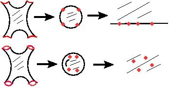
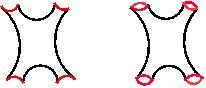
In quantum field theory one calculates correlation functions ⟨ϕ(x1)⋯ϕ(xn)⟩\langle\phi(x_{1})\cdot\cdot\cdot\phi(x_{n})\rangle. To get scattering amplitudes, the correlation functions are put on-shell. In a quantum theory of gravity it is not so clear how to deal with off-shell correlation functions. Instead we can calculate the S-matrix by taking the limit xi→∞x_{i}\to\infty in the correlation functions. In string theory, a drawing of the lowest order interaction of strings looks as in Fig. 7. Unlike QFT there are no interaction vertices, and locally it is a free theory. Only when observed globally the interactions are seen. Taking xi→∞x_{i}\to\infty amounts to taking the legs of the diagram to infinity. The state-operator map says that a state at infinity is equivalent to an insertion of a vertex operator ViV_{i} on the world sheet. A conformal transformation can transform our 2 diagrams into a disk and a sphere. A mobius transformation can transform the disk to the upper half plane, and a stereographic projection takes the sphere to the plane (Fig. 8). The vertex operators will be placed on the boundary of the disk and on the sphere (The sphere obviously has no boundary). Weyl invariance enforces the vertex operators to be on-shell. Higher order diagrams are possible by considering holes and handles in the diagrams for open and closed strings respectively. A scattering amplitude will therefore consist of an expansion in the topology of the world sheet (Fig. 9). Fig. 10 shows the same expansion after performing the conformal transformation.
Refer to caption
Figure 7: Open and closed string diagrams with 4 external particles. The legs should be imagined to continue to infinity.
Refer to caption
Figure 8: Open strings: transforming to the disk and to the complex half-plane. closed strings: transforming to the sphere and to the complex plane.
Refer to caption
Figure 9: Perturbation expansion of the 4-point string amplitudes. Top figure: open strings, bottom figure: closed strings.
Refer to caption
Figure 10: The previous figure after a conformal transformation. For the open string the vertex operators are on the boundary.

We start with the following expression for the scattering amplitude for nn external particles:

ℳn=∑topologiesgs−χ1Vol.∫𝒟X𝒟ge−SP​o​l​yV1⋯Vn\boxed{\mathcal{M}_{n}\ =\ \sum_{\text{topologies}}g_{s}^{-\chi}\ \frac{1}{\text{Vol.}}\int\mathcal{D}X\mathcal{D}g\ e^{-S_{Poly}}\ \ V_{1}\cdot\cdot\cdot V_{n}} (3.20)

Since we are only dealing with tree-level amplitudes, we safely ignored the Faddeev-Popov ghost fields. This equation has the form of an expansion in the string coupling gsg_{s}. There is a functional integration over the coordinate XX, an integration over all possible worldsheet metrics gg, and a sum over the different topologies weighted by gs−χg_{s}^{-\chi}. It is therefore crucial to note that we assume weak coupling.

The Polyakov action in the conformal gauge is:

SP​o​l​y=12​π​α′​∫d2​z​∂X⋅∂¯​XS_{Poly}\ =\ \frac{1}{2\pi\alpha^{\prime}}\int d^{2}z\ \partial X\cdot\bar{\partial}X (3.21)

χ\chi is a topological invariant know as the Euler number:

χ⁡(M)=14​π​∫d2​σ​g​R= 2−2​nh−nb−nc\chi(M)\ =\ \frac{1}{4\pi}\int d^{2}\sigma\sqrt{g}R\ =\ 2-2n_{h}-n_{b}-n_{c} (3.22)

Where nh,nb,ncn_{h},n_{b},n_{c} are the number of handles, boundaries, and cross-caps of the worldsheet. For sphere topology χ=2\chi=2, while for the disk χ=1\chi=1.

We now focus on the lowest order, sphere and disk amplitudes. We need now to integrate over all metrics gg. We transform to the flat metric and recall the remnant global transormations: the conformal killing group P​S​L​(2,C)≡S​L​(2,C)/Z2PSL(2;C)\equiv SL(2;C)/Z_{2} for the sphere, and P​S​L​(2,R)≡S​L​(2,R)/Z2PSL(2;R)\equiv SL(2;R)/Z_{2} for the disk. Technically this means making the following replacements in the path integral:

1Vol.​∫𝒟​g→1Vol.​(S​L​(2,C)CLOSE​∫∏i=1nd2​zi\displaystyle\frac{1}{\text{Vol.}}\int\mathcal{D}g\ \ \ \ \to\ \ \ \ \frac{1}{\text{Vol.}(SL(2;C)}\ \int\prod_{i=1}^{n}d^{2}z_{i}\ \ \ \ \ \ \
1Vol.​∫𝒟​g→1Vol.​(S​L​(2,R)CLOSE​∑{1,…,n}′∫∏i=1nd​zi\displaystyle\frac{1}{\text{Vol.}}\int\mathcal{D}g\ \ \ \ \to\ \ \ \ \frac{1}{\text{Vol.}(SL(2;R)}\ \sum_{{\{1,\ldots,n\}^{\prime}}}\int\prod_{i=1}^{n}dz_{i} (3.23)

For open strings the vertex operators are on the boundary of the disk, and hence have a given ordering to them. A cylic permutation of the vertex operators (which is just a rotation) gives an equivalent configuration because of the reparametrisation invariance of the string action. Hence there should be a sum over the (n−1)!(n-1)! cylic inequivalent permutations. Also note that for open strings there is a single and not a double integration.

We define Vi≡V⁡(zi,ki)V_{i}\equiv V(z_{i},k_{i}) and:

⟨V1⋯Vn⟩≡∫𝒟Xexp(−12​π​α′∫d2z∂X⋅∂¯X)∏i=1nV1⋯Vn\displaystyle\langle V_{1}\cdot\cdot\cdot V_{n}\rangle\ \equiv\ \int\mathcal{D}X\exp\bigg(-\frac{1}{2\pi\alpha^{\prime}}\int d^{2}z\partial X\cdot\bar{\partial}X\bigg)\ \prod_{i=1}^{n}V_{1}\cdot\cdot\cdot V_{n} (3.24)

and we note that The P​S​L​(2,R)PSL(2,R) and P​S​L​(2,C)PSL(2,C) Symmetries on the disk and sphere respectively, allow to fix 3 of the insertion points ziz_{i}. This leaves n−3n-3 integrations in Eq. (3.23). The usual choice is zk=0z_{k}=0 , zl=1z_{l}=1, zm=∞z_{m}=\infty.

We can finally write our master formulas for the closed and open leading order string amplitudes:

ℳ(c​l​o​s​e​d)n=gsn−2Vol.​(S​L​(2,C))∫∏i=1nd2zi⟨V1⋯Vn⟩\boxed{\mathcal{M}^{(closed)}_{n}\ =\ \frac{g_{s}^{n-2}}{\text{Vol.}(SL(2;C))}\ \int\prod_{i=1}^{n}d^{2}z_{i}\ \langle V_{1}\cdot\cdot\cdot V_{n}\rangle} (3.25)
ℳ(o​p​e​n)n=∑{1,…,n}′gsn−1Vol.​(S​L​(2,R))∫∏i=1ndzi⟨V1⋯Vn⟩\boxed{\mathcal{M}^{(open)}_{n}\ =\ \sum_{{\{1,\ldots,n\}^{\prime}}}\frac{g_{s}^{n-1}}{\text{Vol.}(SL(2;R))}\ \int\prod_{i=1}^{n}dz_{i}\ \langle V_{1}\cdot\cdot\cdot V_{n}\rangle} (3.26)

These formulas are valid for any type and any number of external particles. For each particle there corresponds a vertex operator and an integration.

To summarize, the procedure for calculating a scattering amplitude is:

  1. 1.

    Write the vertex functions of the external particles.

  2. 2.

    Calculate the correlator of the vertex functions.

  3. 3.

    Fix 3 of the ziz_{i}’s, and perform the remaining n−3n-3 integrations.

  4. 4.

    For open strings, sum over permutations of the ziz_{i}’s.

3.2.2 Tachyon amplitudes

A simple example is the tachyon (lowest state scalar) scattering amplitude. The vertex function of a tachyon is V⁡(zj,kj)=ei​kj⋅X⁡(zj)V(z_{j},k_{j})=e^{ik_{j}\cdot X(z_{j})}. Defining zi​j≡zi−zjz_{ij}\equiv z_{i}-z_{j}, Eq. (D.8) gives the correlation function for open string tachyons:

⟨ei​k1⋅X⁡(z1)⋯ei​kn⋅X⁡(zn)⟩=∏i<jn|zi​j|2​α′​ki⋅kj\displaystyle\langle e^{ik_{1}\cdot X(z_{1})}\cdots e^{ik_{n}\cdot X(z_{n})}\rangle\ =\ \prod_{i<j}^{n}|z_{ij}|^{2\alpha^{\prime}k_{i}\cdot k_{j}} (3.27)

We now use our freedom to fix 3 ziz_{i}’s. We start by choosing z1=constant>>ziz_{1}=\text{constant}>>z_{i}. This gives:

|z1|2​α′​k1⋅(k2+…+kn)​∏1<i<jn|zi​j|2​α′​ki⋅kj=const.​∏1<i<jn|zi​j|2​α′​ki⋅kj\displaystyle|z_{1}|^{2\alpha^{\prime}k_{1}\cdot(k_{2}+\ldots+k_{n})}\prod_{1<i<j}^{n}|z_{ij}|^{2\alpha^{\prime}k_{i}\cdot k_{j}}\ =\ \text{const.}\prod_{1<i<j}^{n}|z_{ij}|^{2\alpha^{\prime}k_{i}\cdot k_{j}} (3.28)

Where we used k2+⋯+kn=−k1k_{2}+\dots+k_{n}=-k_{1} and k12=m12=constantk_{1}^{2}=m_{1}^{2}=\text{constant}.

Further choosing z2=0,z3=1z_{2}=0,\ z_{3}=1, we get:

ℳn(o​p​e​n)=const.​∫∏l=4nd​zl​|zl|2​α′​k2⋅kl​|1−zl|2​α′​k3⋅kl​∏4≤i<jn|zi​j|2​α′​ki⋅kj\displaystyle\mathcal{M}^{(open)}_{n}\ =\ \text{const.}\int\prod_{l=4}^{n}dz_{l}\ |z_{l}|^{2\alpha^{\prime}k_{2}\cdot k_{l}}|1-z_{l}|^{2\alpha^{\prime}k_{3}\cdot k_{l}}\ \prod_{4\leq i<j}^{n}|z_{ij}|^{2\alpha^{\prime}k_{i}\cdot k_{j}} (3.29)

For closed strings the correlation function is Eq. (D.7), so it is easy to see that:

ℳn(c​l​o​s​e​d)=const.​∫∏l=4nd2​zl​|zl|α′​k2⋅kl​|1−zl|α′​k3⋅kl​∏4≤i<jn|zi​j|α′​ki⋅kj\displaystyle\mathcal{M}^{(closed)}_{n}\ =\ \text{const.}\int\prod_{l=4}^{n}d^{2}z_{l}\ |z_{l}|^{\alpha^{\prime}k_{2}\cdot k_{l}}|1-z_{l}|^{\alpha^{\prime}k_{3}\cdot k_{l}}\ \prod_{4\leq i<j}^{n}|z_{ij}|^{\alpha^{\prime}k_{i}\cdot k_{j}} (3.30)

For n=3n=3 tachyons we get ℳ3=const\mathcal{M}_{3}=\text{const}. Defining s^i​j≡2​α′​ki⋅kj\hat{s}_{ij}\equiv 2\alpha^{\prime}k_{i}\cdot k_{j}, we have for n=4n=4:

ℳ4(o​p​e​n)∝∫d​z​|z|u^​|1−z|s^=B⁡(s^+1,u^+1)\displaystyle\boxed{\mathcal{M}^{(open)}_{4}\ \propto\ \int dz|z|^{\hat{u}}|1-z|^{\hat{s}}\ =\ B(\hat{s}+1,\hat{u}+1)} (3.31)

where B⁡(a,b)=Γ⁡(a)​Γ​(b)Γ⁡(a+b)B(a,b)=\frac{\Gamma(a)\Gamma(b)}{\Gamma(a+b)} is the Beta function.

For the closed string:

ℳ4(c​l​o​s​e​d)∝∫d2​z​|z|u^/2​|1−z|s^/2=Γ⁡(−1−s^4)​Γ​(−1−u^4)​Γ​(3+s^4+u^4)Γ⁡(2+s^4)​Γ​(2+u^4)​Γ​(−2−s^4−u^4)\displaystyle\mathcal{M}^{(closed)}_{4}\ \propto\ \int d^{2}z|z|^{\hat{u}/2}|1-z|^{\hat{s}/2}\ =\ \frac{\Gamma(-1-\frac{\hat{s}}{4})\ \Gamma(-1-\frac{\hat{u}}{4})\ \Gamma(3+\frac{\hat{s}}{4}+\frac{\hat{u}}{4})}{\Gamma(2+\frac{\hat{s}}{4})\ \Gamma(2+\frac{\hat{u}}{4})\ \Gamma(-2-\frac{\hat{s}}{4}-\frac{\hat{u}}{4})} (3.32)

We can write the last equation in a symmetric form. Closed string tachyons have a negative mass of m=−4​Msm=-4M_{s}, hence s^+t^+u^=1Ms2​∑14mj2=−16\hat{s}+\hat{t}+\hat{u}=\frac{1}{M_{s}^{2}}\sum_{1}^{4}m_{j}^{2}=-16. This gives

ℳ4(c​l​o​s​e​d)∝Γ⁡(−1−s^4)​Γ​(−1−t^4)​Γ​(−1−u^4)Γ⁡(2+s^4)​Γ​(2+t^4)​Γ​(2+u^4)\displaystyle\boxed{\mathcal{M}^{(closed)}_{4}\ \propto\ \frac{\Gamma(-1-\frac{\hat{s}}{4})\ \Gamma(-1-\frac{\hat{t}}{4})\ \Gamma(-1-\frac{\hat{u}}{4})}{\Gamma(2+\frac{\hat{s}}{4})\ \Gamma(2+\frac{\hat{t}}{4})\ \Gamma(2+\frac{\hat{u}}{4})}} (3.33)

Eqs. (3.31) and (3.33) are the Veneziano amplitude and the Virasoro-Shapiro amplitude respectively.

3.2.3 Quark-gluon amplitudes

In the previous section we gave tachyons as an example of a scattering amplitude in string theory. Although tachyons are present in bosonic string theory, they are eliminated from the spectrum of string theories which contain world-sheet fermions: superstring theories. In the models we consider, massless fermions and gauge bosons occupy the ground state of the spectrum of the open string. In particular we are interested in quark and gluon scattering amplitudes, and these are calculated quite similarly to tachyons. We recall from section 3.1 that quark-gluon amplitudes may be classified according to weather they are universal or non-universal. Universal amplitudes are defined as those containing 0 or 2 quark (or squark) fields, and non-universal amplitudes are those with more quark fields.

As an example, in order to calculate the nn-point universal amplitudes we need the following correlation functions.

⟨VA(z1)⋯VA(zn)⟩\displaystyle\langle\ V_{A}(z_{1})\ \ \cdots\ V_{A}(z_{n})\ \rangle\ \ \ \ \ \ \ \ \ \ \ \ \ \ \ \ \ \ \ \ \ \ \ \ (3.34)
⟨VA(z1)⋯VA(zn−2)Vψ(zn−1)Vψ¯(zn)⟩\displaystyle\langle\ V_{A}(z_{1})\ \cdots\ V_{A}(z_{n-2})\ \ V_{\psi}(z_{n-1})\ V_{\bar{\psi}}(z_{n})\ \rangle (3.35)

Appendix C lists the vertex functions of gluons and quarks in terms of the fields from the underlying SCFT. Appendix D lists correlation functions of SCFT fields needed in order to calculate the above correlation functions. In Appendix B we present a full calculation of the ℳ⁡(g​g​q​q)\mathcal{M}(ggqq) amplitude. The vertex functions contain the color matrices in such a way that a chain of vertex operators (e.g Eq. (3.34)) gives the Chan-Paton color structure. The Chan-Paton structure is identical to the color decomposition that was done for the field theory amplitudes (Eqs. (3.3), (3.14)). Hence the universal string amplitudes will now be written as1212 12 The Chan-Paton structure relates to open string diagrams as shown in Fig. 11. Each string is assumed to carry a ”‘quark”’ at one end and an ”‘anti-quark”’ at the other end. The quarks being charged and transform as N×N¯N\times\bar{N} under a U⁡(N)U(N) symmetry. To each string there corresponds an N×NN\times N matrix TjiT^{i}_{\ j}. An nn-point amplitude is obtained by contracting in cylic order the ”‘anti-quark”’ index of a string with the ”‘quark”’ index of the next string, and so will contain the factor: (Ta1)lp(Ta2)kl⋯(Tan)pi=Tr[Ta1Ta2⋯Tan]\big(T^{a_{1}}\big)^{p}_{\ \ l}\big(T^{a_{2}}\big)^{l}_{\ k}\cdots\big(T^{a_{n}}\big)^{i}_{\ p}=Tr\big[T^{a_{1}}T^{a_{2}}\cdots T^{a_{n}}\big]. Historically, this picture of a string with a quark and anti-quark at its ends was introduced as a model for mesons, so that U⁡(N)U(N) was the flavor group. This picture remains approximately correct, with the QCD flux tube acting as the string.:

Refer to caption
Figure 11: Chan-Paton structure.
ℳs​t​r​i​n​g(g1,…,gn)=∑{1,…,n}′Tr(Ta1⋯Tan)ms​t​r​i​n​g(g1,…,gn)\boxed{\mathcal{M}_{string}(g_{1},\ldots,g_{n})\ =\ \sum_{\{1,\ldots,n\}^{\prime}}Tr\big(T^{a_{1}}\cdot\cdot\cdot T^{a_{n}}\big)\ m_{string}(g_{1},\dots,g_{n})} (3.36)
ℳs​t​r​i​n​g(q,q¯,g1,…,gn)=∑{1,…,n}(Ta1⋯Tan)i​jms​t​r​i​n​g(q,q¯,g1,…,gn)\boxed{\mathcal{M}_{string}(q,\bar{q},g_{1},\ldots,g_{n})\ =\ \sum_{\{1,\ldots,n\}}\big(T^{a_{1}}\cdot\cdot\cdot T^{a_{n}}\big)_{ij}\ m_{string}(q,\bar{q},g_{1},\ldots,g_{n})} (3.37)

We put the label ”string” because shortly these will be compared to the field theory amplitudes. From Eq. (3.26) the subamplitude is:

ms​t​r​i​n​g=gsn−1Vol.​(S​L​(2,R))∫∏i=1ndzi⟨V~1⋯V~n⟩m_{string}\ =\ \frac{g_{s}^{n-1}}{\text{Vol.}(SL(2;R))}\ \int\prod_{i=1}^{n}dz_{i}\ \langle\widetilde{V}_{1}\cdot\cdot\cdot\widetilde{V}_{n}\rangle (3.38)

and V~i\widetilde{V}_{i} is is just ViV_{i} after stripping it from it’s color matrices.

Following [1, 2], we define mQ​C​Dm_{QCD} as the sub-amplitude in field theory (mm of section 3.1). We can write ms​t​r​i​n​gm_{string} as mQ​C​Dm_{QCD} times a function (form factor) that needs to be calculated. Focusing on the 44 and 55-point helicity amplitudes, the non-MHV subamplitudes vanish also in string theory (Eqs. (3.1) and (3.2)). So we write (and explain afterwords..) for the MHV sub-amplitudes:

  • •

    4 partons

ms​t​r​i​n​g​(g1,g2,g3,g4)=𝔅4​(kj)​mQ​C​D​(g1,g2,g3,g4)\boxed{m_{string}(g_{1},g_{2},g_{3},g_{4})\ \ =\ \ \mathfrak{B}_{4}(k_{j})\ m_{QCD}(g_{1},g_{2},g_{3},g_{4})} (3.39)
ms​t​r​i​n​g​(g1,g2,q3,q¯4)=𝔅4​(kj)​mQ​C​D​(g1,g2,q3,q¯4)\boxed{m_{string}(g_{1},g_{2},q_{3},\bar{q}_{4})\ \ =\ \ \mathfrak{B}_{4}(k_{j})\ m_{QCD}(g_{1},g_{2},q_{3},\bar{q}_{4})} (3.40)
ms​t​r​i​n​g​(q1,q¯2,q3,q¯4)=𝔅^4​(kj,θi)​mQ​C​D​(q1,q¯2,q3,q¯4)\boxed{m_{string}(q_{1},\bar{q}_{2},q_{3},\bar{q}_{4})\ \ =\ \ \widehat{\mathfrak{B}}_{4}(k_{j},\theta_{i})\ m_{QCD}(q_{1},\bar{q}_{2},q_{3},\bar{q}_{4})} (3.41)

Where1313 13 The kinematical factor in front of the integral ensures that 𝔅4→1\mathfrak{B}_{4}\to 1 as s^,u^→1\hat{s},\hat{u}\to 1 so that at low energies ms​t​r​i​n​g→mQ​C​D.m_{string}\to m_{QCD}.

𝔅4​(s^,u^)≡Vt=s^​u^t^​∫01d​z​zs−1​(1−z)u−1\displaystyle\mathfrak{B}_{4}(\hat{s},\hat{u})\ \equiv\ V_{t}\ =\ \frac{\hat{s}\hat{u}}{\hat{t}}\int_{0}^{1}dz\ z^{s-1}(1-z)^{u-1} (3.42)
𝔅^4=s^​u^t^​∫01d​z​zs−1​(1−z)u−1​Iρ​(zi,θj)\displaystyle\widehat{\mathfrak{B}}_{4}\ =\ \frac{\hat{s}\hat{u}}{\hat{t}}\int_{0}^{1}dz\ z^{s-1}(1-z)^{u-1}\ I_{\rho}(z_{i},\theta_{j}) (3.43)

Where IρI_{\rho} is a function which depends on the D-brane setup, and therefore is model dependent.

  • •

    5 partons

ms​t​r​i​n​g​(g1,g2,g3,g4,g5)=𝔅5​(kj)​mQ​C​D​(g1,g2,g3,g4,g5)\boxed{m_{string}(g_{1},g_{2},g_{3},g_{4},g_{5})\ \ =\ \ \mathfrak{B}_{5}(k_{j})\ m_{QCD}(g_{1},g_{2},g_{3},g_{4},g_{5})} (3.44)
ms​t​r​i​n​g​(g1,g2,g3,q4,q¯5)=𝔅5​(kj)​mQ​C​D​(g1,g2,g3,q4,q¯5)\boxed{m_{string}(g_{1},g_{2},g_{3},q_{4},\bar{q}_{5})\ \ =\ \ \mathfrak{B}_{5}(k_{j})\ m_{QCD}(g_{1},g_{2},g_{3},q_{4},\bar{q}_{5})} (3.45)
ms​t​r​i​n​g​(g1,g2,g3,q4,q¯5)=𝔅^5​(kj,θi)​mQ​C​D​(g1,q2,q¯3,q4,q¯5)\boxed{m_{string}(g_{1},g_{2},g_{3},q_{4},\bar{q}_{5})\ \ =\ \ \widehat{\mathfrak{B}}_{5}(k_{j},\theta_{i})\ m_{QCD}(g_{1},q_{2},\bar{q}_{3},q_{4},\bar{q}_{5})} (3.46)

𝔅5\mathfrak{B}_{5} will be given in section 6.3.1.

There are two things to be learned from these equations, showing the special properties of the universal amplitudes.

  1. 1.

    Equality of form factors: a string helicity amplitude is equal to the corresponding field theory amplitude times a stringy form factor. Eqs. (3.39) and (3.40) have the same form factor 𝔅4\mathfrak{B}_{4}, and likewise Eqs. (3.44) and (3.45)) have the same 𝔅5\mathfrak{B}_{5}.

  2. 2.

    Universality: The form factors 𝔅4\mathfrak{B}_{4} and 𝔅5\mathfrak{B}_{5} depend only on the kinematics and hence are universal or model independent. On the other hand, the form factors 𝔅^4\widehat{\mathfrak{B}}_{4} and 𝔅^5\widehat{\mathfrak{B}}_{5} depend on the setup of D-branes and geometry of the extra dimensions, hence they are model dependent or non-universal.

These two properties generalize to nn-point universal amplitudes. The claim is that an nn-point universal helicity amplitude can be written as:

ms​t​r​i​n​g​(g1​…​gn)=𝔅n​(kj)​mQ​C​D​(g1​…​gn)\displaystyle m_{string}(g_{1}\ldots g_{n})\ =\ \mathfrak{B}_{n}(k_{j})\ m_{QCD}(g_{1}\ldots g_{n})\ \ \ \ \ \ \ \ \ \ \ \ \ \ \ \ \ \ \ \ \ \ \ \ \ \ \ (3.47)
ms​t​r​i​n​g​(g1​…​gn−2,qn−1,q¯n)=𝔅n​(kj)​mQ​C​D​(g1​…​gn−2,qn−1,q¯n)\displaystyle m_{string}(g_{1}\ldots g_{n-2},q_{n-1},\bar{q}_{n})\ =\ \mathfrak{B}_{n}(k_{j})\ m_{QCD}(g_{1}\ldots g_{n-2},q_{n-1},\bar{q}_{n}) (3.48)

with the same form factors which depend only on the external momenta, and not on the compactification. Furthermore, 𝔅n\mathfrak{B}_{n} can be expressed in terms of generalized hypergeometric functions, and there are (n−3)!(n-3)! independent sub-amplitudes, see Section 7.

Including the supersymmetric gluino and squark (χ\chi and ϕ\phi), the nn-point universal amplitudes are:

1.m⁡(ga1​…​gan), 3.m⁡(qa1,q¯a2,g3a​…​gan)\displaystyle 1.\ \ m(g^{a_{1}}\ldots g^{a_{n}})\ \ \ \ \ \ \ \ \ \ \ \ \ \ ,\ \ \ \ 3.\ m(q^{a_{1}},\bar{q}^{a_{2}},g^{a}_{3}\ldots g^{a_{n}})
2.m⁡(χa1,χ¯a2,g3a​…​gan), 4.m⁡(ϕa1,ϕ¯a2,g3a​…​gan)\displaystyle 2.\ m(\chi^{a_{1}},\bar{\chi}^{a_{2}},g^{a}_{3}\ldots\ g^{a_{n}})\ \ \ ,\ \ \ \ 4.\ m(\phi^{a_{1}},\bar{\phi}^{a_{2}},g^{a}_{3}\ldots g^{a_{n}}) (3.49)

The universal amplitudes 1 and 2 are related through supersymmetric ward identities, as are amplitudes 3 and 4. In addition, amplitudes 1 and 3 have equal stringy form factors.

3.2.4 Discussion

We further explain the two properties of the universal amplitudes, see [2].

  1. 1.

    Equality of form factors: The explanation is as follows, see Fig. 12. Consider an helicity amplitude with kk quarks and nn gluons: m′​(q1​…​qk,g1​…​gn)m^{\prime}(q_{1}\ldots q_{k},g_{1}\ldots g_{n}) The quarks arise from strings stretched between between 2 stacks of D-branes intersecting at an angle θ\theta. If the angle θ\theta is gradually changed and taken to zero, the quarks will appear as gluinos of the enhanced gauge group Ta⊕TbT^{a}\oplus T^{b}, since the stacks are on top of each other. This new configuration describes an amplitude with kk gluinos and nn gluons: m′′​(χ1​…​χk,g1​…​gn)m^{\prime\prime}(\chi_{1}\ldots\chi_{k},g_{1}\ldots g_{n}). Supersymmetry relates gluinos and gluons, so that m′′m^{\prime\prime} has the same form factor as the all-gluon amplitude m′′′​(g1​…​gk+n)m^{\prime\prime\prime}(g_{1}\ldots g_{k+n}): 𝔅′′=𝔅′′′\mathfrak{B}^{\prime\prime}=\mathfrak{B}^{\prime\prime\prime}. Finally, if k=2k=2 then m′m^{\prime} is a universal amplitude and in particular independent of θ\theta. Hence in this case m′=m′′m^{\prime}=m^{\prime\prime}, and thus 𝔅′=𝔅′′=𝔅′′′\mathfrak{B}^{\prime}=\mathfrak{B}^{\prime\prime}=\mathfrak{B}^{\prime\prime\prime}. We have thus proved that the two types of universal amplitudes have equal form factors.

  2. 2.

    Universality: The most interesting property of these amplitudes is that they are universal or model independent. They are the same in many different models of string theory, because they do not depend on the compactification of the extra dimensions. Universal amplitudes contain only Regge states and not KK or Winding states, which appear in amplitudes with more quarks. KK states arise from the compactification of extra dimensions. Winding states arise when extended objects such as strings or D-branes wrap around the extra dimensions. Regge states are pure string states independent of the extra dimensions.

    Mathematicaly the reason KK and winding states do not appear in the universal amplitudes is the following. KK and winding states only appear in amplitudes constructed from correlators of the boundary changing operators Ξa∩b\Xi^{a\cap b}, and only when there are 4 or more Ξa∩b\Xi^{a\cap b}’s :

    ⟨Ξa∩b(z1)Ξ¯a∩b(z2)⟩=z12−3/4\displaystyle\langle\ \Xi^{a\cap b}(z_{1})\ \bar{\Xi}^{a\cap b}(z_{2})\ \rangle\ =\ z_{12}^{-3/4}\ \ \ \ \ \ \ \ \ \ \ \ \ \ \ \ \ \ \ \ \ \ \ \ \ \ \ \ \ \ \ \ \ \ \ \ \ \ \ \ \ \ \ \ \ \ \ \ \ \ \ \ \ \ \
    ⟨Ξa∩b​(z1)​Ξ¯b∩d​(z2)​Ξd∩c​(z3)​Ξ¯c∩a​(z4)⟩=(z13​z24z12​z14​z23​z34)3/4​Iρ​({zi},θj)\displaystyle\langle\ \Xi^{a\cap b}(z_{1})\ \bar{\Xi}^{b\cap d}(z_{2})\ \Xi^{d\cap c}(z_{3})\ \bar{\Xi}^{c\cap a}(z_{4})\ \rangle\ =\ \Big(\frac{z_{13}z_{24}}{z_{12}z_{14}z_{23}z_{34}}\Big)^{3/4}\ I_{\rho}\ (\{z_{i}\};\theta^{j}) (3.50)

    IρI_{\rho} depends on the compactification and intersections of the D-branes. It includes exchanges of KK and winding states. Since Ξa∩b\Xi^{a\cap b} appears only in the quark vertex function and not in the gluon vertex function (see Eqs. (C.2)-(C.5)), KK and winding states will appear only in amplitudes with 4 or more quarks.

    This property can also be seen diagramatically. Fig. 13 shows the difference, in this respect, between an amplitude containing 2 quarks and an amplitude with 4 quarks. KK and winding states carry internal charge, and charge conservation requires quark pairs on both sides of a KK/winding state line in the diagram. So an amplitude with one quark pair can not have KK/winding state exchange.

Refer to caption
Figure 12: Explanation of the equality of form factors. The 2 quarks of the nn-gluon plus 2-quark amplitude are shown. From left to right: changing the intersection angle until it is zero.
Refer to caption
Figure 13: Explanation of universality. The conservation of internal charge forbids the middle diagram. The same argument holds for the nn-gluon amplitude.

4 4-point amplitudes

Refer to caption
Figure 14: 4 particle kinematics. The scattering angle θ\theta.

4 particle amplitudes are 2→22\to 2 processes at colliders. At the LHC, important signals of 2→22\to 2 processes include: p​p→pp\to 2 jets, p​p→pp\to jet + EW gauge boson and p​p→pp\to 2 EW gauge bosons.

The Mandelstam variables are

s≡(k1+k2)2= 2​k1​k2\displaystyle s\ \equiv\ (k_{1}+k_{2})^{2}\ =\ 2k_{1}k_{2}
t≡(k1+k3)2= 2​k1​k3\displaystyle t\ \equiv\ (k_{1}+k_{3})^{2}\ =\ 2k_{1}k_{3}
u≡(k1+k4)2= 2​k1​k4\displaystyle u\ \equiv\ (k_{1}+k_{4})^{2}\ =\ 2k_{1}k_{4} (4.1)

The kinematics are shown in Fig. 14.

Energy-momentum conservation for massles quarks and gluons gives

s+t+u=∑mi2= 0s+t+u\ =\ \sum m_{i}^{2}\ =\ 0 (4.2)

The hatted Mandelstam variables s^\hat{s}, t^\hat{t}, u^\hat{u} are defined as the Mandelstam variables in units of MsM_{s}:

s^≡s/Ms2=α′​s\displaystyle\hat{s}\ \equiv\ s/M_{s}^{2}\ =\ \alpha^{\prime}s
t^≡t/Ms2=α′​t\displaystyle\hat{t}\ \equiv\ t/M_{s}^{2}\ =\ \alpha^{\prime}t
u^≡u/Ms2=α′​u\displaystyle\hat{u}\ \equiv\ u/M_{s}^{2}\ =\ \alpha^{\prime}u (4.3)

Since this is a scale transformation of the external momenta and since massles QCD/QED are scale invariant, the QCD/QED amplitudes will be invariant under s,t,u→s^,t^,u^s,t,u\to\hat{s},\hat{t},\hat{u}. Amplitudes with WW and ZZ bosons are not scale invariant so that their form will change when passing to the hatted variables. For s,t,u>>MZs,t,u>>M_{Z}, the EW amplitudes become scale invariant as well. The string amplitudes to be discussed later, will obviously change under this scale transformation. These properties are easily seen by looking at the squared amplitudes in sections 4.1 and 4.2.2

4.1 Field theory

References:  [74, 75, 76].

Using the techniques and results of section 3.1, the 4-point squared amplitudes may be computed. As an example, consider the g​g→g​ggg\to gg squared amplitude. Looking at Eq. (3.12) and using ∑si​j4∝(s4+t4+u4)\sum s^{4}_{ij}\propto(s^{4}+t^{4}+u^{4}) and ∑1s12​s23​s34​s41∝1s2​t2+1s2​u2+1u2​t2\sum\frac{1}{s_{12}s_{23}s_{34}s_{41}}\propto\frac{1}{s^{2}t^{2}}+\frac{1}{s^{2}u^{2}}+\frac{1}{u^{2}t^{2}}, we get:

|ℳ|2​(g​g→g​g)∝g4​(s4+t4+u4)​s2+t2+u2s2​t2​u2= 4​g4​[3−t​us2−s​ut2−s​tu2]\displaystyle|\mathcal{M}|^{2}(gg\to gg)\ \propto\ g^{4}(s^{4}+t^{4}+u^{4})\frac{s^{2}+t^{2}+u^{2}}{s^{2}t^{2}u^{2}}\ =\ 4g^{4}\Big[3-\frac{tu}{s^{2}}-\frac{su}{t^{2}}-\frac{st}{u^{2}}\Big] (4.4)

Which is given also in Eq. (4.5). In the last equation we used s+t+u=0s+t+u=0

In the next section we list the squared amplitudes for 2→22\to 2 amplitudes in terms of the Mandelstam variables. Some of the Feynman diagrams are shown in Figs. 15, 16. We consider the processes which are the most important in a hadron collider, namely initial states with a quark or a gluon.

Refer to caption
Figure 15: QCD Feynman diagrams for 4-particles. The other processes can be obtained by crossing.
Refer to caption
Figure 16: Feynman diagrams for partons + photons. The same diagrams describe Z bosons.

4.1.1 The squared amplitudes

  • •

    g​ggg initial state

|ℳ|2​(g​g→g​g)=32​g4​[3−t​us2−s​ut2−s​tu2]|\mathcal{M}|^{2}({\color[rgb]{0,0,1}gg\to gg})\ =\ \frac{3}{2}g^{4}\Big[3-\frac{tu}{s^{2}}-\frac{su}{t^{2}}-\frac{st}{u^{2}}\Big] (4.5)
|ℳ|2​(g​g→g​γ)= 0|\mathcal{M}|^{2}({\color[rgb]{0,0,1}gg\to g\gamma})\ =\ 0 (4.6)
|ℳ|2​(g​g→γ​γ)= 0|\mathcal{M}|^{2}({\color[rgb]{0,0,1}gg\to\gamma\gamma})\ =\ 0 (4.7)
|ℳ|2​(g​g→q​q¯)=38​g4​(t2+u2)​[49​t​u−1s2]|\mathcal{M}|^{2}({\color[rgb]{0,0,1}gg\to q\bar{q}})\ =\ \frac{3}{8}g^{4}(t^{2}+u^{2})\Big[\frac{4}{9tu}-\frac{1}{s^{2}}\Big] (4.8)
  • •

    g​qgq initial state

|ℳ|2​(g​q→g​q)=−g4​(s2+u2)​[49​s​u−1t2]|\mathcal{M}|^{2}({\color[rgb]{0,0,1}gq\to gq})\ =\ -g^{4}(s^{2}+u^{2})\Big[\frac{4}{9su}-\frac{1}{t^{2}}\Big] (4.9)
|ℳ|2​(g​q→γ​q)=−13​g2​e2​s2+u2u​s|\mathcal{M}|^{2}({\color[rgb]{0,0,1}gq\to\gamma q})\ =\ -\frac{1}{3}g^{2}e^{2}\frac{s^{2}+u^{2}}{us} (4.10)
|ℳ|2​(g​q→W​q′)=π​α​αs12​xW​s2+u2+2​MW2​t−s2​u|\mathcal{M}|^{2}({\color[rgb]{0,0,1}gq\to Wq^{\prime}})\ =\ \frac{\pi\alpha\alpha_{s}}{12x_{W}}\ \frac{s^{2}+u^{2}+2M_{W}^{2}t}{-s^{2}u} (4.11)
  • •

    q​q¯q\bar{q} initial state

|ℳ|2​(q​q¯→g​g)=(83)2​|ℳ|2​(g​g→q​q¯)|\mathcal{M}|^{2}({\color[rgb]{0,0,1}q\bar{q}\to gg})\ =\ \Big(\frac{8}{3}\Big)^{2}\ |\mathcal{M}|^{2}(gg\to q\bar{q}) (4.12)
|ℳ|2​(q​q¯→γ​g)=89​g2​e2​t2+u2u​t|\mathcal{M}|^{2}({\color[rgb]{0,0,1}q\bar{q}\to\gamma g})\ =\ \frac{8}{9}g^{2}e^{2}\ \frac{t^{2}+u^{2}}{ut} (4.13)
|ℳ|2​(q​q¯→γ​γ)=34​e4g4​|ℳ|2​(q​q¯→γ​g)|\mathcal{M}|^{2}({\color[rgb]{0,0,1}q\bar{q}\to\gamma\gamma})\ =\ \frac{3}{4}\frac{e^{4}}{g^{4}}\ |\mathcal{M}|^{2}(q\bar{q}\to\gamma g) (4.14)
|ℳ|2​(q​q¯′→W​g)=2​π​α​αs9​xW​(t−MW2)2+(u−MW2)2t​u|\mathcal{M}|^{2}({\color[rgb]{0,0,1}q\bar{q}^{\prime}\to Wg})\ =\ \frac{2\pi\alpha\alpha_{s}}{9x_{W}}\ \frac{(t-M_{W}^{2})^{2}+(u-M_{W}^{2})^{2}}{tu} (4.15)
|ℳ|2​(q​q′¯→q​q′¯)=49​g4​s2+u2t2|\mathcal{M}|^{2}({\color[rgb]{0,0,1}q\bar{q^{\prime}}\to q\bar{q^{\prime}}})\ =\ \frac{4}{9}g^{4}\frac{s^{2}+u^{2}}{t^{2}} (4.16)
|ℳ|2​(q​q¯→q′​q′¯)=49​g4​t2+u2s2|\mathcal{M}|^{2}({\color[rgb]{0,0,1}q\bar{q}\to q^{\prime}\bar{q^{\prime}}})\ =\ \frac{4}{9}g^{4}\frac{t^{2}+u^{2}}{s^{2}} (4.17)
|ℳ|2​(q​q¯→q​q¯)=49​g4​[t2+u2s2+s2+u2t2−2​u23​s​t]|\mathcal{M}|^{2}({\color[rgb]{0,0,1}q\bar{q}\to q\bar{q}})\ =\ \frac{4}{9}g^{4}\Big[\frac{t^{2}+u^{2}}{s^{2}}+\frac{s^{2}+u^{2}}{t^{2}}-\frac{2u^{2}}{3st}\Big] (4.18)
  • •

    q​qqq initial state

|ℳ|2​(q​q→q​q)=49​g4​[s2+t2u2+s2+u2t2−2​s23​t​u]|\mathcal{M}|^{2}({\color[rgb]{0,0,1}qq\to qq})\ =\ \frac{4}{9}g^{4}\Big[\frac{s^{2}+t^{2}}{u^{2}}+\frac{s^{2}+u^{2}}{t^{2}}-\frac{2s^{2}}{3tu}\Big] (4.19)
|ℳ|2​(q​q′→q​q′)=49​g4​s2+u2t2|\mathcal{M}|^{2}({\color[rgb]{0,0,1}qq^{\prime}\to qq^{\prime}})\ =\ \frac{4}{9}g^{4}\frac{s^{2}+u^{2}}{t^{2}} (4.20)

4.2 String theory

4.2.1 The Veneziano amplitude

The Veneziano amplitude VtV_{t}, which enters the 4-point open string scattering amplitudes, is a fantastically rich object. VtV_{t} is the form factor connecting the string and field theory 4-point universal sub-amplitudes, Eqs. (3.39), (3.40), (3.42):

ms​t​r​i​n​g=Vt​mQ​C​D\displaystyle m_{string}=V_{t}\ m_{QCD} (4.21)

Explicitly, the Veneziano amplitude is:

Vt≡s^​u^t^​B​(−s^,−u^)=s^​u^t^​Γ⁡(−s^)​Γ​(−u^)Γ⁡(t^)=Γ⁡(1−s^)​Γ​(1−u^)Γ⁡(1+t^)\displaystyle V_{t}\ \equiv\ \frac{\hat{s}\hat{u}}{\hat{t}}B(-\hat{s},-\hat{u})\ =\ \frac{\hat{s}\hat{u}}{\hat{t}}\frac{\Gamma(-\hat{s})\Gamma(-\hat{u})}{\Gamma(\hat{t})}\ =\ \frac{\Gamma(1-\hat{s})\Gamma(1-\hat{u})}{\Gamma(1+\hat{t})}\ \ \ \ \ \ \ \ \ \ \ \ \ \ \ \ \ \ (4.22)

and by crossing:

Vu≡Vt​(t^↔u^)\displaystyle V_{u}\ \equiv\ V_{t}(\hat{t}\leftrightarrow\hat{u})
Vs≡Vt​(t^↔s^)\displaystyle V_{s}\ \equiv\ V_{t}(\hat{t}\leftrightarrow\hat{s}) (4.23)

The beta function has an integral representation:

B⁡(a,b)≡∫01d​x​xa−1​(1−x)b−1=Γ⁡(a)​Γ​(b)Γ⁡(a+b)\displaystyle B(a,b)\ \equiv\ \int_{0}^{1}dx\ x^{a-1}(1-x)^{b-1}\ =\ \frac{\Gamma{(a)}\Gamma{(b)}}{\Gamma{(a+b)}} (4.24)

One thing to notice is that whereas the field theory tree amplitudes are independent of the collision energy (For massless fermions and gauge bosons.), the string amplitudes do depend on it through the Veneziano amplitude. This means e.g. that the angular distribution of the scattered particles changes as the energy changes.

Properties of the Veneziano factor:

  1. 1.

    Low energy expansion (s^,t^,u^<<1\hat{s},\hat{t},\hat{u}<<1):

    Vt=1+π26​s^​u^+…\displaystyle V_{t}=1+\frac{\pi^{2}}{6}\hat{s}\hat{u}+\ldots (4.25)

    In this limit VtV_{t} is 1 plus corrections in inverse powers of the string scale. See also section 4.2.4.

  2. 2.

    High energy limit (s^>>1\hat{s}>>1).

    There are two types of high energy limits that are usually considered: the fixed scattering angle limit and the Regge limit. In the first case θ=constant\theta=\text{constant} and |s^|,|t^|→∞|\hat{s}|,|\hat{t}|\to\infty. The Regge limit is |s^|→∞|\hat{s}|\to\infty, t^=constant\hat{t}=\text{constant}. From Eqs. (H.27)-(H.29) we have:

    Fixed angle limit:

    Vt,Vu,Vs⟶e−f⁡(θ)​s\displaystyle V_{t},V_{u},V_{s}\ \ \ \longrightarrow\ \ \ e^{-f(\theta)s} (4.26)

    Regge limit:

    Vu,Vs⟶s−t\displaystyle V_{u},V_{s}\ \ \ \longrightarrow\ \ \ s^{-t}
    Vt⟶e−f⁡(θ)​s\displaystyle V_{t}\ \ \ \longrightarrow\ \ \ e^{-f(\theta)s} (4.27)

    Where,

    f⁡(θ)=(1−cos⁡θ2)​ln⁡(1−cos⁡θ2)+(1+cos⁡θ2)​ln⁡(1+cos⁡θ2)\displaystyle f(\theta)\ =\ \Big(\frac{1-\cos\theta}{2}\Big)\ln\Big(\frac{1-\cos\theta}{2}\Big)\ +\ \Big(\frac{1+\cos\theta}{2}\Big)\ln\Big(\frac{1+\cos\theta}{2}\Big) (4.28)

    In the fixed angle limit, VtV_{t} is exponentially decreasing. This is extremely soft UV behavior.

  3. 3.

    s-channel pole expansion:

    VtV_{t} can be expanded on s-channel poles, giving rise to the most useful equation of this work:

    Vt=−s^​u^t^∑n=0∞1n!1s^−n∏K=1n(u^+K)\boxed{V_{t}\ =\ -\frac{\hat{s}\hat{u}}{\hat{t}}\ \sum_{n=0}^{\infty}\frac{1}{n!}\ \frac{1}{\hat{s}-n}\ \prod_{K=1}^{n}(\hat{u}+K)} (4.29)

    There are simple s-channel poles at each integer nn:

    s=n​Ms2\displaystyle s\ =\ nM_{s}^{2} (4.30)

    Notice that the residue is a function of u^\hat{u} only (mind the simple factor in front of the sum..).

  4. 4.

    D.H.S duality:

    Vt​(−s^,−u^)=Vt​(−u^,−s^)\displaystyle V_{t}(-\hat{s},-\hat{u})=V_{t}(-\hat{u},-\hat{s}) (4.31)

    Thus Eq. (4.29) can then be written as a sum of u-channel poles.

    Vt=−s^​u^t^∑n=0∞1n!1u^−n∏K=1n(s^+K)V_{t}\ =\ -\frac{\hat{s}\hat{u}}{\hat{t}}\ \sum_{n=0}^{\infty}\frac{1}{n!}\ \frac{1}{\hat{u}-n}\ \prod_{K=1}^{n}(\hat{s}+K) (4.32)

    We will almost always use the s-channel pole expansion though.

  5. 5.

    Positivity of the residues: ”The no-ghost theorem”:

    For VtV_{t} to describe a scattering amplitude, the residues of the poles must be positive. This is difficult to prove, and it is correct only if the dimensions of space-time are D=26D=26 or D=10D=10, for the bosonic and super-string respectively.

  6. 6.

    Polynomial residues and spins:

    The residue of the pole contains the angular part of the amplitude, which determines the spins of the exchanged resonances. If the residue is a polynomial in cos⁡θ\cos\theta of degree kk, then there can be exchanges of spins from 00 to kk. It is seen from Eq. (4.29) that the residue is a polynomial of degree nn in u^\hat{u} or equivalently in cos⁡θ\cos\theta.

    Res(Vt)∝∏K=0n−1(u^+K)=u^(u^+1)⋯(u^+n−1)=∑p=1napu^p=∑p=1nbpcospθ\displaystyle Res(V_{t})\propto\prod_{K=0}^{n-1}(\hat{u}+K)=\hat{u}(\hat{u}+1)\cdots(\hat{u}+n-1)=\sum_{p=1}^{n}a_{p}\hat{u}^{p}=\sum_{p=1}^{n}b_{p}\cos^{p}\theta (4.33)

    Where apa_{p} and bpb_{p} are constants.

    VtV_{t} is the form factor which multiplies mQ​C​Dm_{QCD} (Eq. (4.21)), which itself depends on cos⁡θ\cos\theta. The angular dependency in mQ​C​Dm_{QCD} can shift the minimum and maximum spins, so that in general:

    0+J0≤J≤n+J0′\displaystyle 0+J_{0}\ \leq\ J\ \leq\ n+J^{\prime}_{0} (4.34)

From Eq. (4.30), there are exchanges of of an infinite number of resonances with masses (Fig. 17):

mn=n​Ms\displaystyle m_{n}\ \ =\ \ \sqrt{n}\ M_{s} (4.35)

These are string excitations called Regge states.

Refer to caption
Figure 17: s-channel Regge state exchange.
Refer to caption
Figure 18: Left: The spectrum of Regge excitations of the gluon: gn​Jg^{nJ}. Right: Regge excitations of the quark: qn​Jq^{nJ}. Linear Regge trajectories are also shown.

We will see that the Regge excitations of the gluon (which we denote by gn​Jg^{nJ}) have, at a mass level nn, spins in the range:

0≤J≤n+1\displaystyle 0\leq\ J\ \leq n+1 (4.36)

These gn​Jg^{nJ} particles are exchanged e.g. in g​g→g​ggg\to gg. The spectrum of gn​Jg^{nJ} states can be plotted on the n−Jn-J plane as in Fig. 18.

In sections 3.2.3, 3.2.4 we mentioned that the processes g​g→g​ggg\to gg and g​q→g​qgq\to gq have the same form factor VtV_{t}. So the amplitude for g​q→g​qgq\to gq will also have an infinity of poles, corresponding to the Regge excitations of the quark qn​Jq^{nJ} (Fig. 18). The figure also shows Regge trajectories which have the form J=J0+α′​mn2=J0+nJ=J_{0}+\alpha^{\prime}m_{n}^{2}=J_{0}+n, where J0=0​ or ​1/2J_{0}=0\text{ or }1/2 for gn​Jg^{nJ} and qn​Jq^{nJ} respectively.

Near a resonance, one term in the sum of Eq. (4.29) is dominant:

Vt→s^→n1(n−1)!​1s^−n​u^​∏K=1n−1(u^+K)\displaystyle V_{t}\ \ \xrightarrow{\hat{s}\to n}\ \ \frac{1}{(n-1)!}\ \frac{1}{\hat{s}-n}\ \hat{u}\prod_{K=1}^{n-1}(\hat{u}+K)
Vu→s^→n(−1)n−1(n−1)!​1s^−n​t^​∏K=1n−1(u^+K)\displaystyle V_{u}\ \ \xrightarrow{\hat{s}\to n}\ \ \frac{(-1)^{n-1}}{(n-1)!}\ \frac{1}{\hat{s}-n}\ \hat{t}\prod_{K=1}^{n-1}(\hat{u}+K) (4.37)

In contrast to VtV_{t} and VuV_{u}, VsV_{s} is finite (has no s-channel poles):

Vs→s^→nΓ⁡(1−t^)​Γ​(1−u^)Γ⁡(1+n)=finite\displaystyle V_{s}\ \ \xrightarrow{\hat{s}\to n}\ \ \frac{\Gamma(1-\hat{t})\Gamma(1-\hat{u})}{\Gamma(1+n)}\ =\ \text{finite} (4.38)

so near a resonance of the amplitude we can neglect VsV_{s} terms.

An interesting property can be seen:

VuVt=Γ⁡(1−t^)​Γ​(1+t^)Γ⁡(1−u^)​Γ​(1+u^)=t^​sin⁡(π​u^)u^​sin⁡(π​t^)\displaystyle\frac{V_{u}}{V_{t}}=\frac{\Gamma(1-\hat{t})\ \Gamma(1+\hat{t})}{\Gamma(1-\hat{u})\ \Gamma(1+\hat{u})}=\frac{\hat{t}\ \sin(\pi\hat{u})}{\hat{u}\ \sin(\pi\hat{t})} (4.39)

near a pole this becomes:

VuVt=(−1)n−1​u^t^,when ​s^→n\displaystyle\frac{V_{u}}{V_{t}}\ =\ (-1)^{n-1}\frac{\hat{u}}{\hat{t}}\ \ \ ,\ \ \ \text{when }\hat{s}\to n (4.40)

From Eq. (4.37) the previous equation is seen to be equivalent to:

∏K=1n−1(u^+K)=(−1)n−1​∏K=1n−1(t^+K),when ​s^→n\displaystyle\prod_{K=1}^{n-1}(\hat{u}+K)\ =\ (-1)^{n-1}\prod_{K=1}^{n-1}(\hat{t}+K)\ \ \ ,\ \ \ \text{when }\hat{s}\to n (4.41)

4.2.2 The squared amplitudes

References: squared amplitudes from [1].

In Appendix B we give an example of a full calculation of a squared amplitude. In this section we write down the string squared amplitudes just as we did in the field theory case. The Veneziano factors will be written explicitly in terms of the Mandelstam variables. It is then immediately seen that some the processes have only n=n=odd resonances (the residues vanish for n=n=even). This is explained in section 5.2.4 and Appendix A.

We denote by AA the U⁡(1)U(1) gauge boson from the stack aa (the color stack), and by BB the non-abelian gauge boson from stack bb.

  • •

    g​ggg initial state

|ℳ|2​(g​g→g​g)=\displaystyle|\mathcal{M}|^{2}({\color[rgb]{0,0,1}gg\to gg})\ \ =\ \ \ \ \ \ \ \ \ \ \ \ \ \ \ \ \ \ \ \ \ \ \ \ \ \ \ \ \ \ \ \ \ \ \ \ \ \ \ \ \ \ \ \ \ \ \ \ \ \ \ \ \ \ \ \ \ \ \ \ \ \ \
g4​(1s2+1t2+1u2)​[94​(s2​Vs2+t2​Vt2+u2​Vu2)−13​(s​Vs+t​Vt+u​Vu)2]\displaystyle g^{4}\Big(\frac{1}{s^{2}}+\frac{1}{t^{2}}+\frac{1}{u^{2}}\Big)\Big[\frac{9}{4}\big(s^{2}V_{s}^{2}+t^{2}V_{t}^{2}+u^{2}V_{u}^{2}\big)\ -\ \frac{1}{3}\big(sV_{s}+tV_{t}+uV_{u}\big)^{2}\Big]
=n4+u^4+t^4n2​(s^−n)2​g4(n−1)!2​[∏K=1n−1(u^+K)2]⋅{19/12,odd​n9/4,even​n}.\displaystyle=\ \frac{n^{4}+\hat{u}^{4}+\hat{t}^{4}}{n^{2}(\hat{s}-n)^{2}}\ \frac{g^{4}}{(n-1)!^{2}}\ \Bigg[\prod_{K=1}^{n-1}(\hat{u}+K)^{2}\Bigg]\cdot\begin{Bmatrix}19/12,&\textrm{odd}\ n\\ 9/4,&\textrm{even}\ n\end{Bmatrix}. (4.42)
|ℳ|2​(g​g→g​A)=56​g4​QA2​(1s2+1t2+1u2)​(s​Vs+t​Vt+u​Vu)2\displaystyle|\mathcal{M}|^{2}({\color[rgb]{0,0,1}gg\to gA})=\frac{5}{6}g^{4}Q_{A}^{2}\ \Big(\frac{1}{s^{2}}+\frac{1}{t^{2}}+\frac{1}{u^{2}}\Big)\big(sV_{s}+tV_{t}+uV_{u}\big)^{2}
=5​g4​QA23​n4+u^4+t^4n2​(s^−n)2​1(n−1)!2​[∏K=1n−1(u^+K)2]⋅{1,odd n0,even n}.\displaystyle=\frac{5g^{4}Q_{A}^{2}}{3}\ \frac{n^{4}+\hat{u}^{4}+\hat{t}^{4}}{n^{2}(\hat{s}-n)^{2}}\ \frac{1}{(n-1)!^{2}}\ \Bigg[\prod_{K=1}^{n-1}(\hat{u}+K)^{2}\Bigg]\cdot\begin{Bmatrix}1,&\textrm{odd $n$}\\ 0,&\textrm{even $n$}\end{Bmatrix}. (4.43)
|ℳ|2​(g​g→A​A)=125​QA2​|ℳ|2​(g​g→g​A)\displaystyle|\mathcal{M}|^{2}({\color[rgb]{0,0,1}gg\to AA})\ \ =\ \ \frac{12}{5}Q_{A}^{2}\ |\mathcal{M}|^{2}(gg\to gA) (4.44)
|ℳ|2​(g​g→q​q¯)=g4​t2+u2s2​[16​u​t​(t​Vt+u​Vu)2−38​Vt​Vu]\displaystyle|\mathcal{M}|^{2}({\color[rgb]{0,0,1}gg\to q\bar{q}})\ =\ g^{4}\frac{t^{2}+u^{2}}{s^{2}}\ \Big[\frac{1}{6ut}\big(tV_{t}+uV_{u}\big)^{2}-\frac{3}{8}V_{t}V_{u}\Big]
=u^​t^​(u^2+t^2)n2​(s^−n)2​g4(n−1)!2​[∏K=1n−1(u^+K)2]⋅{7/24,odd n25/24,even n}.\displaystyle=\frac{\hat{u}\hat{t}(\hat{u}^{2}+\hat{t}^{2})}{n^{2}(\hat{s}-n)^{2}}\ \frac{g^{4}}{(n-1)!^{2}}\ \Bigg[\prod_{K=1}^{n-1}(\hat{u}+K)^{2}\Bigg]\cdot\begin{Bmatrix}7/24,&\textrm{odd $n$}\\ 25/24,&\textrm{even $n$}\end{Bmatrix}. (4.45)
  • •

    g​qgq initial state

|ℳ|2​(g​q→g​q)=g4​s2+u2t2​[Vs​Vu−49​1s​u​(s​Vs+u​Vu)2]\displaystyle|\mathcal{M}|^{2}({\color[rgb]{0,0,1}gq\to gq})\ =\ g^{4}\frac{s^{2}+u^{2}}{t^{2}}\ \Big[V_{s}V_{u}-\frac{4}{9}\frac{1}{su}\ \big(sV_{s}+uV_{u}\big)^{2}\Big]
=−4​g49u^​(u^2+n2)n​(s^−n)21(n−1)!2∏K=1n−1(u^+K)2\displaystyle=-\frac{4g^{4}}{9}\ \frac{\hat{u}(\hat{u}^{2}+n^{2})}{n(\hat{s}-n)^{2}}\ \frac{1}{(n-1)!^{2}}\ \prod_{K=1}^{n-1}(\hat{u}+K)^{2} (4.46)
|ℳ|2​(g​q→A​q)=−g43​QA2​s2+u2s​u​t2​(s​Vs2+u​Vu2)\displaystyle|\mathcal{M}|^{2}({\color[rgb]{0,0,1}gq\to Aq})\ =\ \frac{-g^{4}}{3}Q_{A}^{2}\ \frac{s^{2}+u^{2}}{sut^{2}}\ \big(sV_{s}^{2}+uV_{u}^{2}\big)
=−13​g4​QA2​u^​(u^2+n2)n​(s^−n)2​1(n−1)!2​∏K=1n−1(u^+K)2\displaystyle=\frac{-1}{3}g^{4}Q_{A}^{2}\ \frac{\hat{u}(\hat{u}^{2}+n^{2})}{n(\hat{s}-n)^{2}}\ \frac{1}{(n-1)!^{2}}\ \prod_{K=1}^{n-1}(\hat{u}+K)^{2} (4.47)
|ℳ|2​(g​q→B​q′)=−g46​|Tq​q¯′B|2​s2+u2s​u​Vt2\displaystyle|\mathcal{M}|^{2}({\color[rgb]{0,0,1}gq\to Bq^{\prime}})\ =\ \frac{-g^{4}}{6}|T^{B}_{q\bar{q}^{\prime}}|^{2}\ \frac{s^{2}+u^{2}}{su}\ V_{t}^{2}
=−g46​|Tq​q¯′B|2​u^​(u^2+n2)n​(s^−n)2​1(n−1)!2​∏K=1n−1(u^+K)2\displaystyle=\frac{-g^{4}}{6}|T^{B}_{q\bar{q}^{\prime}}|^{2}\ \frac{\hat{u}(\hat{u}^{2}+n^{2})}{n(\hat{s}-n)^{2}}\ \frac{1}{(n-1)!^{2}}\ \prod_{K=1}^{n-1}(\hat{u}+K)^{2} (4.48)
  • •

    q​q¯q\bar{q} initial state

|ℳ|2​(q​q¯→g​g)=(83)2​|ℳ|2​(g​g→q​q¯)\displaystyle|\mathcal{M}|^{2}({\color[rgb]{0,0,1}q\bar{q}\to gg})\ \ =\ \ \Big(\frac{8}{3}\Big)^{2}\ |\mathcal{M}|^{2}(gg\to q\bar{q}) (4.49)
|ℳ|2(qq¯→gA)=g489QA2t2+u2t​u​s2(tVt+uVu)2=\displaystyle|\mathcal{M}|^{2}({\color[rgb]{0,0,1}q\bar{q}\to gA})\ \ =\ \ g^{4}\frac{8}{9}Q_{A}^{2}\ \frac{t^{2}+u^{2}}{tus^{2}}\ \big(tV_{t}+uV_{u}\big)^{2}=\ \ \ \ \ \ \ \ \ \ \ \ \ \
329​g4​QA2​u^​t^​(u^2+t^2)n2​(s^−n)2​1(n−1)!2​[∏K=1n−1(u^+K)2]⋅{1,odd n0,even n}.\displaystyle\frac{32}{9}g^{4}Q_{A}^{2}\ \frac{\hat{u}\hat{t}(\hat{u}^{2}+\hat{t}^{2})}{n^{2}(\hat{s}-n)^{2}}\ \frac{1}{(n-1)!^{2}}\ \Bigg[\prod_{K=1}^{n-1}(\hat{u}+K)^{2}\Bigg]\cdot\begin{Bmatrix}1,&\textrm{odd $n$}\\ 0,&\textrm{even $n$}\end{Bmatrix}. (4.50)
|ℳ|2​(q​q¯→A​A)=34​QA2​|ℳ|2​(q​q¯→g​A)\displaystyle|\mathcal{M}|^{2}({\color[rgb]{0,0,1}q\bar{q}\to AA})\ \ =\ \ \frac{3}{4}Q_{A}^{2}\ |\mathcal{M}|^{2}(q\bar{q}\to gA) (4.51)
|ℳ|2​(q​q¯→g​B)=g4​49​|Tq​q¯B|2​QA2​t2+u2t​u​Vs2|\mathcal{M}|^{2}({\color[rgb]{0,0,1}q\bar{q}\to gB})\ \ =\ \ g^{4}\frac{4}{9}|T^{B}_{q\bar{q}}|^{2}Q_{A}^{2}\ \frac{t^{2}+u^{2}}{tu}\ V_{s}^{2} (4.52)
|ℳ|2​(q​q¯→B​A)=34​QA2​|ℳ|2​(q​q¯→g​B)|\mathcal{M}|^{2}({\color[rgb]{0,0,1}q\bar{q}\to BA})\ \ =\ \ \frac{3}{4}Q_{A}^{2}\ |\mathcal{M}|^{2}(q\bar{q}\to gB) (4.53)
  • •

    q​qqq initial state

|ℳ|2(qq→qq)=g4{291t2[(sFt​ub​b)2+(sFt​uc​c)2+(uGt​ub′​c)2+(uGt​uc′​b)2]+\displaystyle|\mathcal{M}|^{2}({\color[rgb]{0,0,1}qq\to qq})\ =\ g^{4}\bigg\{\frac{2}{9}\ \frac{1}{t^{2}}\Big[(sF_{tu}^{bb})^{2}+(sF_{tu}^{cc})^{2}+(uG_{tu}^{{}^{\prime}bc})^{2}+(uG_{tu}^{{}^{\prime}cb})^{2}\Big]+
291u2[(sFu​tb​b)2+(sFu​tc​c)2+(tGu​tb′​c)2+(tGu​tc′​b)2]−427s2t​u(Ft​ub​bFu​tb​b+Ft​uc​cFu​tc​c)}\displaystyle\frac{2}{9}\ \frac{1}{u^{2}}\Big[(sF_{ut}^{bb})^{2}+(sF_{ut}^{cc})^{2}+(tG_{ut}^{{}^{\prime}bc})^{2}+(tG_{ut}^{{}^{\prime}cb})^{2}\Big]-\frac{4}{27}\ \frac{s^{2}}{tu}\big(F_{tu}^{bb}F_{ut}^{bb}+F_{tu}^{cc}F_{ut}^{cc}\big)\bigg\} (4.54)
|ℳ|2​(q​q′→q​q′)=2​g49​1t2​[(s​Ft​ub​b)2+(s​Gt​uc​c′)2+(u​Gt​ub′​c)2+(u​Gt​ub′​c′)2]|\mathcal{M}|^{2}({\color[rgb]{0,0,1}qq^{\prime}\to qq^{\prime}})\ =\ \frac{2g^{4}}{9}\ \frac{1}{t^{2}}\Big[(sF_{tu}^{bb})^{2}+(sG_{tu}^{cc^{\prime}})^{2}+(uG_{tu}^{{}^{\prime}bc})^{2}+(uG_{tu}^{{}^{\prime}bc^{\prime}})^{2}\Big] (4.55)

See [1] for further details on quark-quark scattering.

Let us note a few things that can be seen from these squared amplitudes:

  • •

    As seen in Eqs. (4.43), (4.44), (4.50), (4.51), amplitudes with a g​AgA or A​AAA in the final state do not have n=e​v​e​nn=even poles. This happens because of the vanishing of the following color factors: f0​a​b=f00​a=f000=0f^{0ab}=f^{00a}=f^{000}=0. See also section 5.2.4 and Appendix A.

  • •

    Taking the leading term near a pole, we see that there are 3 classes of amplitudes:

    1. 1.

      g​q→g​qgq\to gq , g​q→A​qgq\to Aq , g​q→B​q′gq\to Bq^{\prime} are proportional near a pole.

    2. 2.

      g​g→g​ggg\to gg , g​g→g​Agg\to gA , and g​g→A​Agg\to AA are proportional near a pole (the latter two vanish at n=e​v​e​nn=even poles.).

    3. 3.

      g​g→q​q¯gg\to q\bar{q} , q​q¯→g​gq\bar{q}\to gg , q​q¯→g​Aq\bar{q}\to gA , and q​q¯→A​Aq\bar{q}\to AA are proportional near a pole (the latter two vanish at n=e​v​e​nn=even poles.).

    Moreover, these 3 classes differ (near a pole) only by a simple kinematic factor: u^​(u^2+n2)\hat{u}(\hat{u}^{2}+n^{2}) , (n4+u^4+t^4)(n^{4}+\hat{u}^{4}+\hat{t}^{4}) , u^​t^​(u^2+t^2)\hat{u}\hat{t}(\hat{u}^{2}+\hat{t}^{2}) for the first, second, and third class respectively.

4.2.3 The softened squared amplitudes

The simple poles of the amplitudes are given finite widths via the Breit-Wigner form as in section 5.1.1. Following for example [11], we write the softened squared amplitudes for exchange of Regge states from the first excited state n=1n=1. The Regge states with quantum numbers (n,J)(n,J) are written as: gn,J,An,J,qn,Jg^{n,J},A^{n,J},q^{n,J}, recall also Fig. 18.

  • •

    g​ggg initial state

|ℳ|2(gg→gg)=19​g412{Wgn,Jg​g→g​g[1(s^−1)2+(Γg1,0/Ms)2+t^4+u^4(s^−1)2+(Γg1,2/Ms)2]\displaystyle|\mathcal{M}|^{2}({\color[rgb]{0,0,1}gg\to gg})=\frac{19g^{4}}{12}\Bigg\{\ W_{g^{n,J}}^{gg\to gg}\bigg[\frac{1}{(\hat{s}-1)^{2}+(\Gamma_{g^{1,0}}/M_{s})^{2}}+\frac{\hat{t}^{4}+\hat{u}^{4}}{(\hat{s}-1)^{2}+(\Gamma_{g^{1,2}}/M_{s})^{2}}\bigg]
+WAn,Jg​g→g​g[1(s^−1)2+(ΓA1,0/Ms)2+t^4+u^4(s^−1)2+(ΓA1,2/Ms)2]}\displaystyle+W_{A^{n,J}}^{gg\to gg}\bigg[\frac{1}{(\hat{s}-1)^{2}+(\Gamma_{A^{1,0}}/M_{s})^{2}}+\frac{\hat{t}^{4}+\hat{u}^{4}}{(\hat{s}-1)^{2}+(\Gamma_{A^{1,2}}/M_{s})^{2}}\bigg]\ \Bigg\} (4.56)
|ℳ|2​(g​g→g​A)=53​g4​QA2​[1(s^−1)2+(Γg1,0/Ms)2+u^4+t^4(s^−1)2+(Γg1,2/Ms)2]\displaystyle|\mathcal{M}|^{2}({\color[rgb]{0,0,1}gg\to gA})\ =\ \frac{5}{3}g^{4}Q_{A}^{2}\Bigg[\frac{1}{(\hat{s}-1)^{2}+(\Gamma_{g^{1,0}}/M_{s})^{2}}+\frac{\hat{u}^{4}+\hat{t}^{4}}{(\hat{s}-1)^{2}+(\Gamma_{g^{1,2}}/M_{s})^{2}}\Bigg] (4.57)
|ℳ|2​(g​g→A​A)= 4​g4​QA4​[1(s^−1)2+(ΓA1,0/Ms)2+u^4+t^4(s^−1)2+(ΓA1,2/Ms)2]\displaystyle|\mathcal{M}|^{2}({\color[rgb]{0,0,1}gg\to AA})\ =\ 4g^{4}Q_{A}^{4}\Bigg[\frac{1}{(\hat{s}-1)^{2}+(\Gamma_{A^{1,0}}/M_{s})^{2}}+\frac{\hat{u}^{4}+\hat{t}^{4}}{(\hat{s}-1)^{2}+(\Gamma_{A^{1,2}}/M_{s})^{2}}\Bigg] (4.58)
|ℳ|2​(g​g→q​q¯)=724​g4​Nf​{Wgn,Jg​g→q​q¯​u^​t^​(u^2+t^2)(s^−1)2+(Γg1,2/Ms)2+WAn,Jg​g→q​q¯​u^​t^​(u^2+t^2)(s^−1)2+(ΓA1,2/Ms)2}\displaystyle|\mathcal{M}|^{2}({\color[rgb]{0,0,1}gg\to q\bar{q}})=\frac{7}{24}g^{4}N_{f}\bigg\{W_{g^{n,J}}^{gg\to q\bar{q}}\frac{\hat{u}\hat{t}(\hat{u}^{2}+\hat{t}^{2})}{(\hat{s}-1)^{2}+(\Gamma_{g^{1,2}}/M_{s})^{2}}+W_{A^{n,J}}^{gg\to q\bar{q}}\frac{\hat{u}\hat{t}(\hat{u}^{2}+\hat{t}^{2})}{(\hat{s}-1)^{2}+(\Gamma_{A^{1,2}}/M_{s})^{2}}\bigg\}
  • •

    g​qgq initial state

|ℳ|2​(g​q→g​q)=−4​g49​[u^(s^−1)2+(Γq1,12/Ms)2+u^3(s^−1)2+(Γq1,32/Ms)2]\displaystyle|\mathcal{M}|^{2}({\color[rgb]{0,0,1}gq\to gq})=-\frac{4g^{4}}{9}\Bigg[\frac{\hat{u}}{(\hat{s}-1)^{2}+(\Gamma_{q^{1,\frac{1}{2}}}/M_{s})^{2}}+\frac{\hat{u}^{3}}{(\hat{s}-1)^{2}+(\Gamma_{q^{1,\frac{3}{2}}}/M_{s})^{2}}\Bigg] (4.60)
|ℳ|2​(g​q→A​q)=−13​g4​QA2​[u^(s^−1)2+(Γq1,12/Ms)2+u^3(s^−1)2+(Γq1,32/Ms)2]\displaystyle|\mathcal{M}|^{2}({\color[rgb]{0,0,1}gq\to Aq})=-\frac{1}{3}g^{4}Q_{A}^{2}\Bigg[\frac{\hat{u}}{(\hat{s}-1)^{2}+(\Gamma_{q^{1,\frac{1}{2}}}/M_{s})^{2}}+\frac{\hat{u}^{3}}{(\hat{s}-1)^{2}+(\Gamma_{q^{1,\frac{3}{2}}}/M_{s})^{2}}\Bigg] (4.61)
|ℳ|2​(g​q→B​q′)=−16​g4​|Tq​q¯′B|2​[u^(s^−1)2+(Γq1,12/Ms)2+u^3(s^−1)2+(Γq1,32/Ms)2]\displaystyle|\mathcal{M}|^{2}({\color[rgb]{0,0,1}gq\to Bq^{\prime}})=-\frac{1}{6}g^{4}|T^{B}_{q\bar{q}^{\prime}}|^{2}\Bigg[\frac{\hat{u}}{(\hat{s}-1)^{2}+(\Gamma_{q^{1,\frac{1}{2}}}/M_{s})^{2}}+\frac{\hat{u}^{3}}{(\hat{s}-1)^{2}+(\Gamma_{q^{1,\frac{3}{2}}}/M_{s})^{2}}\Bigg] (4.62)
  • •

    q​q¯q\bar{q} initial state

|ℳ|2​(q​q¯→g​g)=5627​g4​{Wgn,Jq​q¯→g​g​u^​t^​(u^2+t^2)(s^−1)2+(Γg1,2/Ms)2+WAn,Jq​q¯→g​g​u^​t^​(u^2+t^2)(s^−1)2+(ΓA1,2/Ms)2}\displaystyle|\mathcal{M}|^{2}({\color[rgb]{0,0,1}q\bar{q}\to gg})=\frac{56}{27}g^{4}\bigg\{W_{g^{n,J}}^{q\bar{q}\to gg}\frac{\hat{u}\hat{t}(\hat{u}^{2}+\hat{t}^{2})}{(\hat{s}-1)^{2}+(\Gamma_{g^{1,2}}/M_{s})^{2}}+W_{A^{n,J}}^{q\bar{q}\to gg}\frac{\hat{u}\hat{t}(\hat{u}^{2}+\hat{t}^{2})}{(\hat{s}-1)^{2}+(\Gamma_{A^{1,2}}/M_{s})^{2}}\bigg\}
|ℳ|2​(q​q¯→g​A)=329​g4​QA2​u^​t^​(u^2+t^2)(s^−1)2+(Γg1,2/Ms)2\displaystyle|\mathcal{M}|^{2}({\color[rgb]{0,0,1}q\bar{q}\to gA})=\frac{32}{9}g^{4}Q_{A}^{2}\frac{\hat{u}\hat{t}(\hat{u}^{2}+\hat{t}^{2})}{(\hat{s}-1)^{2}+(\Gamma_{g^{1,2}}/M_{s})^{2}} (4.64)
|ℳ|2​(q​q¯→A​A)=83​g4​QA4​u^​t^​(u^2+t^2)(s^−1)2+(ΓA1,2/Ms)2\displaystyle|\mathcal{M}|^{2}({\color[rgb]{0,0,1}q\bar{q}\to AA})=\frac{8}{3}g^{4}Q_{A}^{4}\frac{\hat{u}\hat{t}(\hat{u}^{2}+\hat{t}^{2})}{(\hat{s}-1)^{2}+(\Gamma_{A^{1,2}}/M_{s})^{2}} (4.65)

Where the widths are:

Γg1,0=g24​π​N4​Ms≈ 0.075​Ms\displaystyle\Gamma_{g^{1,0}}\ =\ \frac{g^{2}}{4\pi}\ \frac{N}{4}\ M_{s}\ \approx\ 0.075\ M_{s} (4.66)
ΓA1,0=g24​π​N2​Ms≈ 0.15​Ms\displaystyle\Gamma_{A^{1,0}}\ =\ \frac{g^{2}}{4\pi}\ \frac{N}{2}\ M_{s}\ \approx\ 0.15\ M_{s} (4.67)
Γg1,2=g24​π​(N10+Nf40)​Ms≈ 0.045​Ms\displaystyle\Gamma_{g^{1,2}}\ =\ \frac{g^{2}}{4\pi}\ \Big(\frac{N}{10}+\frac{N_{f}}{40}\Big)\ M_{s}\ \approx\ 0.045\ M_{s} (4.68)
ΓA1,2=g24​π​(N5+Nf40)​Ms≈ 0.075​Ms\displaystyle\Gamma_{A^{1,2}}\ =\ \frac{g^{2}}{4\pi}\ \Big(\frac{N}{5}+\frac{N_{f}}{40}\Big)\ M_{s}\ \approx\ 0.075\ M_{s} (4.69)
Γq1,12=Γq1,32=g24​π​N8​Ms≈ 0.038​Ms\displaystyle\Gamma_{q^{1,\frac{1}{2}}}\ =\ \Gamma_{q^{1,\frac{3}{2}}}\ =\ \frac{g^{2}}{4\pi}\ \frac{N}{8}\ M_{s}\ \approx\ 0.038\ M_{s} (4.70)

and the right hand side was obtained by setting αs=g2/4​π≈0.1\alpha_{s}=g^{2}/4\pi\approx 0.1, N=3N=3, and Nf=6N_{f}=6.

We now write the relative weights between exchange of an S​U​(N)SU(N) and U⁡(1)U(1) gauge bosons.

Wgn​Jg​g→g​g=(N2−1)​(Γgn​J→g​g)2(N2−1)​(Γgn​J→g​g)2+(ΓAn​J→g​g)2={11+4​(N2−1)(N2−4)2=2557,n=o​d​d 1,n=e​v​e​n}\displaystyle W_{g^{nJ}}^{gg\to gg}=\frac{(N^{2}-1)(\Gamma_{g^{nJ}\to gg})^{2}}{(N^{2}-1)(\Gamma_{g^{nJ}\to gg})^{2}+(\Gamma_{A^{nJ}\to gg})^{2}}\ =\ \begin{Bmatrix}\frac{1}{1+\frac{4(N^{2}-1)}{(N^{2}-4)^{2}}}=\frac{25}{57}\ ,\ n=odd\\ \ \ \ \ \ \ \ \ \ \ \ \ \ \ \ \ \ 1\ ,\ n=even\end{Bmatrix} (4.71)
WAn​Jg​g→g​g=1−Wgn​Jg​g→g​g=(ΓAn​J→g​g)2(N2−1)​(Γgn​J→g​g)2+(ΓAn​J→g​g)2={3257,n=o​d​d 0,n=e​v​e​n}\displaystyle W_{A^{nJ}}^{gg\to gg}=1-W_{g^{nJ}}^{gg\to gg}=\frac{(\Gamma_{A^{nJ}\to gg})^{2}}{(N^{2}-1)(\Gamma_{g^{nJ}\to gg})^{2}+(\Gamma_{A^{nJ}\to gg})^{2}}\ =\ \begin{Bmatrix}\frac{32}{57}\ ,\ n=odd\\ \ 0\ ,\ n=even\end{Bmatrix} (4.72)
Wgn​Jg​g→q​q¯=Wgn​Jq​q¯→g​g=(N2−1)​Γgn​J→g​g​Γgn​J→q​q¯(N2−1)​Γgn​J→g​g​Γgn​J→q​q¯+ΓAn​J→g​g​ΓAn​J→q​q¯=\displaystyle W_{g^{nJ}}^{gg\to q\bar{q}}=W_{g^{nJ}}^{q\bar{q}\to gg}=\frac{(N^{2}-1)\Gamma_{g^{nJ}\to gg}\Gamma_{g^{nJ}\to q\bar{q}}}{(N^{2}-1)\Gamma_{g^{nJ}\to gg}\Gamma_{g^{nJ}\to q\bar{q}}+\Gamma_{A^{nJ}\to gg}\Gamma_{A^{nJ}\to q\bar{q}}}\ =\
{11+2N2−4=57,n=o​d​d 1,n=e​v​e​n}\displaystyle\begin{Bmatrix}\frac{1}{1+\frac{2}{N^{2}-4}}=\frac{5}{7}\ ,\ n=odd\\ \ \ \ \ \ \ \ \ \ \ \ \ \ 1\ ,\ n=even\end{Bmatrix} (4.73)
WAn​Jg​g→q​q¯=WAn​Jq​q¯→g​g=1−Wgn​Jg​g→q​q¯=ΓAn​J→g​g​ΓAn​J→q​q¯(N2−1)​Γgn​J→g​g​Γgn​J→q​q¯+ΓAn​J→g​g​ΓAn​J→q​q¯=\displaystyle W_{A^{nJ}}^{gg\to q\bar{q}}=W_{A^{nJ}}^{q\bar{q}\to gg}=1-W_{g^{nJ}}^{gg\to q\bar{q}}=\frac{\Gamma_{A^{nJ}\to gg}\Gamma_{A^{nJ}\to q\bar{q}}}{(N^{2}-1)\Gamma_{g^{nJ}\to gg}\Gamma_{g^{nJ}\to q\bar{q}}+\Gamma_{A^{nJ}\to gg}\Gamma_{A^{nJ}\to q\bar{q}}}\ =\
{27,n=o​d​d0,n=e​v​e​n}\displaystyle\begin{Bmatrix}\frac{2}{7}\ ,\ n=odd\\ 0\ ,\ n=even\end{Bmatrix} (4.74)

Where we put N=3N=3 on the right hand side, and the decay widths are taken from sections 5.2.4 and 5.2.5. The weights are independent of nn and JJ, they only differ for n=o​d​dn=odd and n=e​v​e​nn=even.

Now we that we have seen the n=1n=1 case, we jump a little bit ahead of time and give the prescription for arbitrary nn and JJ. A general helicity amplitude will have the following form near a resonance of mass squared mn2=s^=nm_{n}^{2}=\hat{s}=n, see Eq. (5.11):

ℳm,m′=1(s^−n)+i⁡(Γgn​J/Ms)​A​∑JCm,m′n,J​dm,m′J​(θ)\displaystyle\mathcal{M}_{m,m^{\prime}}\ =\ \frac{1}{(\hat{s}-n)+i(\Gamma_{g^{nJ}}/M_{s})}\ A\ \sum_{J}C^{n,J}_{m,m^{\prime}}\ d^{J}_{m,m^{\prime}}(\theta) (4.75)

We wrote this with gn​Jg^{nJ}, but the same form will hold also for qn​Jq^{nJ}.

The amplitude can then be squared:

|ℳm,m′|2=A2​∑J1,J2Cm,m′n,J1​Cm,m′n,J2​dm,m′J1​dm,m′J2(s^−n)2+Γgn​J1​Γgn​J2/Ms2\displaystyle|\mathcal{M}_{m,m^{\prime}}|^{2}\ =\ A^{2}\sum_{J_{1},J_{2}}C^{n,J_{1}}_{m,m^{\prime}}\ C^{n,J_{2}}_{m,m^{\prime}}\ \frac{d^{J_{1}}_{m,m^{\prime}}\ d^{J_{2}}_{m,m^{\prime}}}{(\hat{s}-n)^{2}+\Gamma_{g^{nJ_{1}}}\ \Gamma_{g^{nJ_{2}}}/M_{s}^{2}} (4.76)

Eq. (I.10) shows that dd’s are orthogonal, therefore the interference terms vanish in the total cross section:

σm,m′=∫−11d​cos⁡θ32​π​s​|ℳm,m′|2=A232​π​s​∑J(Cm,m′n,J)2​42​J+1(s^−n)2+(Γgn​J/Ms)2\displaystyle\sigma_{m,m^{\prime}}\ =\ \int_{-1}^{1}\frac{d\cos\theta}{32\pi s}|\mathcal{M}_{m,m^{\prime}}|^{2}\ =\ \frac{A^{2}}{32\pi s}\sum_{J}\big(C^{n,J}_{m,m^{\prime}}\big)^{2}\ \frac{\frac{4}{2J+1}}{(\hat{s}-n)^{2}+(\Gamma_{g^{nJ}}/M_{s})^{2}} (4.77)

The amplitudes having exchanges of gn​Jg^{nJ} (as opposed to qn​Jq^{nJ}) have also the opposite helicity configuration ℳm,−m′\mathcal{M}_{m,-m^{\prime}}. In this case, when the two squared amplitudes are added we get:

|ℳm,m′|2+|ℳm,−m′|2=A2​∑J1,J2Cm,m′n,J1​Cm,m′n,J2​[dm,m′J1​dm,m′J2+(−1)J1+J2​dm,−m′J1​dm,−m′J2(s^−n)2+Γgn​J1​Γgn​J2/Ms2]\displaystyle|\mathcal{M}_{m,m^{\prime}}|^{2}+|\mathcal{M}_{m,-m^{\prime}}|^{2}=A^{2}\sum_{J_{1},J_{2}}C^{n,J_{1}}_{m,m^{\prime}}\ C^{n,J_{2}}_{m,m^{\prime}}\ \bigg[\frac{d^{J_{1}}_{m,m^{\prime}}d^{J_{2}}_{m,m^{\prime}}+(-1)^{J_{1}+J_{2}}\ d^{J_{1}}_{m,-m^{\prime}}d^{J_{2}}_{m,-m^{\prime}}}{(\hat{s}-n)^{2}+\Gamma_{g^{nJ_{1}}}\ \Gamma_{g^{nJ_{2}}}/M_{s}^{2}}\bigg] (4.78)

Where Eqs. (5.28), (5.29) were used.

4.2.4 Low energy limit

References:  [1, 71, 72].

When the center of mass energy is significantly lower than the string scale, s<<Ms2s<<M_{s}^{2}, the string amplitudes coincide with the standard model ones. In this section we calculate the first stringy correction to the standard model amplitudes.

The Veneziano amplitudes can be expanded in powers of α′=1/Ms2\alpha^{\prime}=1/M_{s}^{2}. To order α′7\alpha^{\prime 7}:

1s​t​Vu=1s​t−α′2​π26−α′3​(s+t)​ζ​(3)−α′4​π4360​(4​s2+s​t+4​t2)+\displaystyle\frac{1}{st}V_{u}\ =\ \frac{1}{st}-\alpha^{\prime 2}\frac{\pi^{2}}{6}-\alpha^{\prime 3}(s+t)\zeta(3)-\alpha^{\prime 4}\frac{\pi^{4}}{360}(4s^{2}+st+4t^{2})+\ \ \ \ \ \ \ \ \ \ \ \ \ \ \ \ \ \ \ \ \ \ \ \ \ \ \ \ \
α′5​[π26​s​t​(s+t)​ζ​(3)−(s+t)​(s2+s​t+t2)​ζ​(5)]−\displaystyle\alpha^{\prime 5}\Big[\frac{\pi^{2}}{6}st(s+t)\zeta(3)-(s+t)(s^{2}+st+t^{2})\zeta(5)\Big]-\ \ \ \ \ \ \ \ \ \ \ \ \ \ \ \ \ \ \ \ \ \ \ \ \ \ \ \ \ \ \ \ \ \ \ \ \ \ \ \ \ \ \ \ \ \ \ \
α′6[π61512016s4+12s3t+23s2t2+12st3+16t4)−12st(s+t)2ζ(3)2]+\displaystyle\alpha^{\prime 6}\Big[\frac{\pi^{6}}{15120}16s^{4}+12s^{3}t+23s^{2}t^{2}+12st^{3}+16t^{4})-\frac{1}{2}st(s+t)^{2}\zeta(3)^{2}\Big]+\ \ \ \ \ \ \ \ \ \ \ \ \ \ \ \ \ \ \ \ \ \
α′7​[π4360​s​t​(s+t)​(4​s2+s​t+4​t2)​ζ​(3)+π26​s​t​(s2+s​t+t2)​ζ​(5)−(s2+s​t+t2)​ζ​(7)]+…\displaystyle\alpha^{\prime 7}\Big[\frac{\pi^{4}}{360}st(s+t)(4s^{2}+st+4t^{2})\zeta(3)+\frac{\pi^{2}}{6}st(s^{2}+st+t^{2})\zeta(5)-(s^{2}+st+t^{2})\zeta(7)\Big]+...

We note that the α′\alpha^{\prime} correction vanishes. We will need only up to α′3\alpha^{\prime 3} order1414 14 In this equation, the α′2\alpha^{\prime 2} correction can be shown to arise from the following effective lagrangian: ℐF4=−α′2​π26Tr[Fμ1​μ2Fμ2​μ3Fμ3​μ4Fμ4​μ1+2Fμ1​μ2Fμ3​μ4Fμ2​μ3Fμ4​μ1−\displaystyle\mathcal{I}_{F^{4}}=-\frac{\alpha^{\prime 2}\pi^{2}}{6}Tr\Big[F_{\mu_{1}\mu_{2}}F_{\mu_{2}\mu_{3}}F_{\mu_{3}\mu_{4}}F_{\mu_{4}\mu_{1}}+2F_{\mu_{1}\mu_{2}}F_{\mu_{3}\mu_{4}}F_{\mu_{2}\mu_{3}}F_{\mu_{4}\mu_{1}}- 14Fμ1​μ2Fν1​ν2Fμ2​μ1Fν2​ν1−12Fμ1​μ2Fμ2​μ1Fν1​ν2Fν2​ν1]\displaystyle\frac{1}{4}F_{\mu_{1}\mu_{2}}F_{\nu_{1}\nu_{2}}F_{\mu_{2}\mu_{1}}F_{\nu_{2}\nu_{1}}-\frac{1}{2}F_{\mu_{1}\mu_{2}}F_{\mu_{2}\mu_{1}}F_{\nu_{1}\nu_{2}}F_{\nu_{2}\nu_{1}}\Big] (4.80) :

Vt= 1−[π26​s​u]​α′2−[ζ⁡(3)​s​t​u]​α′3​…\displaystyle V_{t}\ =\ 1-\Big[\frac{\pi^{2}}{6}su\Big]\alpha^{\prime 2}-[\zeta(3)stu]\alpha^{\prime 3}\ldots
Vu= 1−[π26​s​t]​α′2−[ζ⁡(3)​s​t​u]​α′3​…\displaystyle V_{u}\ =\ 1-\Big[\frac{\pi^{2}}{6}st\Big]\alpha^{\prime 2}-[\zeta(3)stu]\alpha^{\prime 3}\ldots
Vs= 1−[π26​t​u]​α′2−[ζ⁡(3)​s​t​u]​α′3​…\displaystyle V_{s}\ =\ 1-\Big[\frac{\pi^{2}}{6}tu\Big]\alpha^{\prime 2}-[\zeta(3)stu]\alpha^{\prime 3}\ldots (4.81)

We write |ℳ|2=|ℳ|S​M2+Δ​|ℳ|2|\mathcal{M}|^{2}=|\mathcal{M}|^{2}_{SM}+\Delta|\mathcal{M}|^{2}, where |ℳ|S​M2|\mathcal{M}|^{2}_{SM} is the standard model squared amplitude and Δ​|ℳ|2\Delta|\mathcal{M}|^{2} is the first correction. The first corrections to the squared amplitudes of section 4.2.2 are:

  • •

    g​ggg initial state

Δ​|ℳ|2​(g​g→g​g)=−2​g4​ζ​(3)​s​t​u​92​[3−t​us2−u​st2−t​su2]​α′3\Delta|\mathcal{M}|^{2}({\color[rgb]{0,0,1}gg\to gg})\ =\ -2g^{4}\zeta(3)stu\frac{9}{2}\Big[3-\frac{tu}{s^{2}}-\frac{us}{t^{2}}-\frac{ts}{u^{2}}\Big]\ \alpha^{\prime 3} (4.82)
Δ​|ℳ|2​(g​g→g​A)=5​π4​g4​QA224​(s2​t2+s2​u2+u2​t2)​α′4\Delta|\mathcal{M}|^{2}({\color[rgb]{0,0,1}gg\to gA})\ =\ \frac{5\pi^{4}g^{4}Q_{A}^{2}}{24}\ (s^{2}t^{2}+s^{2}u^{2}+u^{2}t^{2})\ \alpha^{\prime 4} (4.83)
Δ​|ℳ|2​(g​g→A​A)=π4​g4​QA42​(s2​t2+s2​u2+u2​t2)​α′4\Delta|\mathcal{M}|^{2}({\color[rgb]{0,0,1}gg\to AA})\ =\ \frac{\pi^{4}g^{4}Q_{A}^{4}}{2}\ (s^{2}t^{2}+s^{2}u^{2}+u^{2}t^{2})\ \alpha^{\prime 4} (4.84)
Δ​|ℳ|2​(g​g→q​q¯)=g4​π23​(u2+t2)​α′2\Delta|\mathcal{M}|^{2}({\color[rgb]{0,0,1}gg\to q\bar{q}})\ =\ \frac{g^{4}\pi^{2}}{3}\ (u^{2}+t^{2})\ \alpha^{\prime 2} (4.85)
  • •

    g​qgq initial state

Δ​|ℳ|2​(g​q→g​q)=π2​g4​QA43​(u2+s2)​α′2\Delta|\mathcal{M}|^{2}({\color[rgb]{0,0,1}gq\to gq})\ =\ \frac{\pi^{2}g^{4}Q_{A}^{4}}{3}\ (u^{2}+s^{2})\ \alpha^{\prime 2} (4.86)
Δ​|ℳ|2​(g​q→A​q)=−2​g4​π29​(u2+s2)​α′2\Delta|\mathcal{M}|^{2}({\color[rgb]{0,0,1}gq\to Aq})\ =\ \frac{-2g^{4}\pi^{2}}{9}\ (u^{2}+s^{2})\ \alpha^{\prime 2} (4.87)
Δ​|ℳ|2​(g​q→B​q′)=g4​π218​|Tq​q¯B|2​(u2+s2)​α′2\Delta|\mathcal{M}|^{2}({\color[rgb]{0,0,1}gq\to Bq^{\prime}})\ =\ \frac{g^{4}\pi^{2}}{18}|T^{B}_{q\bar{q}}|^{2}\ (u^{2}+s^{2})\ \alpha^{\prime 2} (4.88)
  • •

    q​q¯q\bar{q} initial state

Δ​|ℳ|2​(q​q¯→g​g)=64​g4​π227​(u2+t2)​α′2\Delta|\mathcal{M}|^{2}({\color[rgb]{0,0,1}q\bar{q}\to gg})\ =\ \frac{64g^{4}\pi^{2}}{27}\ (u^{2}+t^{2})\ \alpha^{\prime 2} (4.89)
Δ​|ℳ|2​(q​q¯→g​A)=8​π4​g4​QA281​u​t​(u2+t2)​α′4\Delta|\mathcal{M}|^{2}({\color[rgb]{0,0,1}q\bar{q}\to gA})\ =\ \frac{8\pi^{4}g^{4}Q_{A}^{2}}{81}\ ut(u^{2}+t^{2})\ \alpha^{\prime 4} (4.90)
Δ​|ℳ|2​(q​q¯→A​A)=2​π4​g4​QA427​u​t​(u2+t2)​α′4\Delta|\mathcal{M}|^{2}({\color[rgb]{0,0,1}q\bar{q}\to AA})\ =\ \frac{2\pi^{4}g^{4}Q_{A}^{4}}{27}\ ut(u^{2}+t^{2})\ \alpha^{\prime 4} (4.91)
Δ​|ℳ|2​(q​q¯′→g​B)=−4​g4​π4​|Tq​q¯B|227​u​t​(u2+t2)​α′2\Delta|\mathcal{M}|^{2}({\color[rgb]{0,0,1}q\bar{q}^{\prime}\to gB})\ =\ \frac{-4g^{4}\pi^{4}|T^{B}_{q\bar{q}}|^{2}}{27}\ ut(u^{2}+t^{2})\ \alpha^{\prime 2} (4.92)
Δ​|ℳ|2​(q​q¯′→B​A)=−g4​π4​|Tq​q¯B|2​QA29​u​t​(u2+t2)​α′2\Delta|\mathcal{M}|^{2}({\color[rgb]{0,0,1}q\bar{q}^{\prime}\to BA})\ =\ \frac{-g^{4}\pi^{4}|T^{B}_{q\bar{q}}|^{2}Q_{A}^{2}}{9}\ ut(u^{2}+t^{2})\ \alpha^{\prime 2} (4.93)

We note that for all the processes with a final state AA, the first correction is α′4\alpha^{\prime 4}. The correction for gluon scattering is α′3\alpha^{\prime 3}, and all the rest are α′2\alpha^{\prime 2} .

4.3 Collider phenomenology

References:  [73, 74, 77, 78, 79, 80, 81, 82, 1, 2, 3, 4, 5, 6, 7, 8, 9, 10, 11, 19, 20, 94, 95, 96, 97, 98].

The calculation of a cross section d​σ~d\widetilde{\sigma} is done by convoluting the partonic cross section d​σ​(i​j→k​l)d\sigma(ij\to kl) with the parton distribution functions of the two colliding protons:

𝑑σ~=∫01∫01d​xa​d​xb​∑i​j​k​lfi​(xa,M)​fj​(xb,M)​𝑑σ​(i​j→k​l)\displaystyle d\widetilde{\sigma}=\int_{0}^{1}\int_{0}^{1}dx_{a}\ dx_{b}\sum_{ijkl}\ f_{i}(x_{a},M)\ f_{j}(x_{b},M)\ d\sigma(ij\to kl) (4.94)

The partonic cross section and the squared amplitude are related:

|ℳ⁡(i​j→k​l)|2= 64​π2​s​d​σd​Ω= 16​π​s2​d​σd​t|\mathcal{M}(ij\to kl)|^{2}\ =\ 64\pi^{2}s\ \frac{d\sigma}{d\Omega}\ =\ 16\pi s^{2}\ \frac{d\sigma}{dt} (4.95)

A useful form for the dijet cross section is given in Eq. (G.23). The dijet cross section can thus be calculated in field theory and in string theory, using the squared amplitudes written earlier. As is well known, the field theory cross section is a smooth power-law decreasing function. The string theory cross section exhibits bumps at s=n​Ms2s=nM_{s}^{2}, and these are clear signals of new physics. If the string scale is higher then the collision energy then these bumps cannot be seen, but smooth deviations from the field theory cross section can still be searched for (e.g. contact interaction searches).

Another useful type of analysis are dijet angular distributions. Angular distributions are a sensitive probe of new physics since QCD dijets are more central (because of the t-channel poles) whereas new physics tend to be more isotropic. Most importantly, angular distributions are a way to probe exchanges of different spins. Therefore they can be used to differentiate e.g a bump coming from a spin 2 KK graviton, from Regge state exchange of different spins.

The ratio RR is a useful measure of angular distributions:

R=d​σd​M​(|y1|,|y2|<0.5)d​σd​M​(0.5<|y1|,|y2|<1)R\ =\ \frac{\frac{d\sigma}{dM}(|y_{1}|,|y_{2}|<0.5)}{\frac{d\sigma}{dM}(0.5<|y_{1}|,|y_{2}|<1)} (4.96)

It also has the benefit that systematic uncertainties, such as the jet energy scale (JES), tend to cancel in the ratio.

It is very important that the following 4-fermion processes, which are non-universal amplitudes, are suppressed at the LHC:

q​q¯→q​q¯\displaystyle q\ \bar{q}\to q\ \bar{q}
q​q→q​q\displaystyle q\ q\to q\ q (4.97)

The first process is suppressed because q¯\bar{q} has low luminosity in proton collisions, and the second process does not have s-channel Regge state exchange. Therefore, the universal (model independent) amplitudes will dominate the dijet signal.

Looking at the squared amplitudes of section 4.2.2, we note the following things:

  1. 1.

    The process p+p→γ/Z+J​e​tp+p\rightarrow\gamma/Z+Jet has even resonances only from the partonic process g​q→A​qgq\rightarrow Aq. This means that the even resonances of a γ/Z+J​e​t\gamma/Z+Jet signal are a probe of the Regge excitations of the quarks.

  2. 2.

    The process p+p→W+J​e​tp+p\rightarrow W+Jet has resonances only from the partonic process g​q→B​q′gq\rightarrow Bq^{\prime}.

  3. 3.

    The process p+p→γ/Z+γ/Zp+p\rightarrow\gamma/Z+\gamma/Z has only odd resonances.

Possibilities for collider phenomenology other then virtual exchange of Regge states include:

  • •

    Direct production of a Regge state in the final state, section 8 and [20].

  • •

    Multi-jets in the final state, beginning with the 3-jet signal. The squared amplitudes of [2] and section 6.3.3 can be used for this purpose.

  • •

    Phenomenology at a lepton collider or photon collider, [8]. For example the process γ+γ→γ+γ\gamma+\gamma\to\gamma+\gamma exhibits tree level Regge state exchange.

  • •

    Signals other then Regge states include: production of ZZ’ bosons coming from the extra U⁡(1)U(1)’s of D-brane models (section 2.4 and [10]). Also signals arising from the presence of extra dimensions: KK and winding state exchange and production, miniature black hole production and Hawking radiation etc..

4.3.1 Constraints from the LHC

The most directly related limit is from the CMS experiment [93]: exclusion of string resonances from dijet mass distribution with 1​f​b−11\ fb^{-1}:

Ms> 4​T​e​V\displaystyle\boxed{M_{s}\ >\ 4\ TeV} (4.98)

We list some additional constraints which have some relevance for us.

  • •

    [93] CMS limits from dijets searches with 1​f​b−11\ fb^{-1} :

    - Bound on the mass of excited quarks:

    Mq∗>2.49​T​e​VM_{q^{*}}>2.49\ TeV .

    - Bound on the mass of axigluons:

    M>2.47​T​e​VM>2.47\ TeV .

  • •

    [78], [79] CMS lower limit on quark contact interaction scale for left handed quarks via dijet angular distributions with 36​p​b−136\ pb^{-1} :

    Λ>5.6−6.7​T​e​V\Lambda>5.6-6.7\ TeV .

  • •

    [106] ATLAS limits from dijet searches with 0.81​f​b−10.81\ fb^{-1}:

    - Bound on excited quarks:

    Mq∗>2.91​T​e​VM_{q^{*}}>2.91\ TeV .

    -Bound on axigluons:

    M>3.21​T​e​VM>3.21\ TeV .

  • •

    [80], [81], [82] ATLAS limits from dijet mass and angular distributions with 36​p​b−136\ pb^{-1} (distributions measured up to ∼3.5​T​e​V\sim 3.5\ TeV):

    - Exclusion of quantum gravity scales from Randall-Meade quantum black holes:

    0.75<mD<3.67​T​e​V0.75<m_{D}<3.67\ TeV .

    - Limit on quark contact interactions:

    Λ>9.5​T​e​V\Lambda>9.5\ TeV .

Another way to discover new physics is by measuring the couplings of the Higgs boson, which (Maybe) was recently discovered at the LHC [110, 111] and Tevatron[112]. See for example [car].

5 Decay widths

References:  [1, 7, 19, 73]. After the submission of this article, [104] appeared which deals with related issues.

In this section we suggest several methods to compute decay widths of Regge states. The basic idea is that of [7], in which a tree level amplitude is factorized into two trilinear couplings connected by an s-channel resonance (see e.g the s-channel diagram of Fig. 1). This is e.g similar to the tree level production of a standard model ZZ boson. In field theory, 1-loop corrections give an imaginary part to the amplitude which causes the resonance to decay. As we will shortly see, the optical theorem enables to compute the decay widths from tree level amplitudes.

This technique is basically field theoretical. 1-loop amplitudes can also be computed in string theory. This is beyond the scope this work.

5.1 Setting the stage

5.1.1 The Breit-Wigner form

In order to compare a squared amplitude to scattering experiments, the decay width of the exchanged particles must be taken in to account. Recall that the string amplitudes exhibit an infinite sum of poles of the type ∼1s−n​Ms2\sim\frac{1}{s-nM_{s}^{2}} corresponding to exchange of Regge states with zero decay width. Higher order corrections will produce a finite decay width Γ\Gamma, causing a Breit-Wigner softening of the poles:

1s−n​Ms2→1s−n​Ms2+i​Γ​Ms\displaystyle\frac{1}{s-nM_{s}^{2}}\to\frac{1}{s-nM_{s}^{2}+i\Gamma M_{s}} (5.1)

The squared amplitude will then be

∼1(s−n​Ms2)2+(Γ​Ms)2\displaystyle\sim\frac{1}{(s-nM_{s}^{2})^{2}+(\Gamma M_{s})^{2}} (5.2)
Refer to caption
Figure 19: The full propagator.

We now derive this, following [73]. In field theory (for example ϕ3\phi^{3} theory) a tree level s-channel exchange of a resonance is of the form  1s−M02\frac{1}{s-M_{0}^{2}}. Radiative corrections will remove the pole at s=M02s=M_{0}^{2}. If Π⁡(s)\Pi(s) is the 1PI radiative correction to the tree propagator then the full propagator will be Fig. 19:

1s−M02⟶1s−M02+1s−M02Π(s)1s−M02+…=\displaystyle\frac{1}{s-M_{0}^{2}}\ \ \longrightarrow\ \ \frac{1}{s-M_{0}^{2}}+\frac{1}{s-M_{0}^{2}}\Pi(s)\frac{1}{s-M_{0}^{2}}+\ldots\ =
1s−M02​[1−Π⁡(s)s−M02+(Π⁡(s)s−M02)2+…]=1s−M02−Π⁡(s)\displaystyle\frac{1}{s-M_{0}^{2}}\bigg[1-\frac{\Pi(s)}{s-M_{0}^{2}}+\Big(\frac{\Pi(s)}{s-M_{0}^{2}}\Big)^{2}+\ldots\bigg]=\frac{1}{s-M_{0}^{2}-\Pi(s)} (5.3)

The physical mass is determined by:

M2−M02−R​e​Π​(M2)=0\displaystyle M^{2}-M_{0}^{2}-Re\ \Pi(M^{2})=0 (5.4)

Using the fact that near the pole we have s≈M2s\approx M^{2}, we get

M2−M02−Π⁡(s)=s−M02−[R​e​Π​(M2)+R​e​Π​(s)′|s=M2​(s−M2)]+i​I​m​Π​(M2)=\displaystyle M^{2}-M_{0}^{2}-\Pi(s)=s-M_{0}^{2}-\big[Re\ \Pi(M^{2})+Re\ \Pi(s)^{\prime}|_{s=M^{2}}(s-M^{2})\big]+iIm\ \Pi(M^{2})=
[1+R​e​Π​(s)′|s=M2]​(s−M2)+i​I​m​Π​(M2)=\displaystyle\big[1+Re\ \Pi(s)^{\prime}|_{s=M^{2}}\big](s-M^{2})+iIm\ \Pi(M^{2})=
𝒵−1​(s−M2)+i​I​m​Π​(M2)=𝒵−1​[(s−M2)+i​M​Γ]\displaystyle\mathcal{Z}^{-1}(s-M^{2})+iIm\ \Pi(M^{2})=\mathcal{Z}^{-1}\big[(s-M^{2})+iM\Gamma\big] (5.5)

Where 𝒵\mathcal{Z} is the field strength renormalization and in the last equation we used:

ImΠ(M2)=−𝒵−12∑f1,f2∫d3​k1(2​π)3​2​E1d3​k2(2​π)3​2​E2|ℳ¯|2(Z→f1f2)=−𝒵−1MΓ\displaystyle Im\ \Pi(M^{2})=-\frac{\mathcal{Z}^{-1}}{2}\sum_{f_{1},f_{2}}\int\frac{d^{3}k_{1}}{(2\pi)^{3}2E_{1}}\ \frac{d^{3}k_{2}}{(2\pi)^{3}2E_{2}}|\overline{\mathcal{M}}|^{2}(Z\to f_{1}f_{2})=-\mathcal{Z}^{-1}M\Gamma (5.6)

We finally achieved:

1s−M02⟶𝒵s−M2+i​M​Γ\displaystyle\frac{1}{s-M_{0}^{2}}\ \ \longrightarrow\ \ \frac{\mathcal{Z}}{s-M^{2}+iM\Gamma} (5.7)

5.1.2 Amplitudes in terms of the dd-functions

In order to exhibit the exchange of resonances, a given amplitude should be expanded in terms of the physical states, i.e states with a definite spin. Put differently, the amplitude needs to be expanded on the basis of Wigner dd-functions.

Therefore we write an helicity amplitude as:

ℳm,m′=ℳ⁡(12→34)=∑J∗ℳ⁡(12→J∗→34)\mathcal{M}_{m,m^{\prime}}=\mathcal{M}(12\to 34)=\sum_{J^{*}}\mathcal{M}(12\to J^{*}\to 34) (5.8)

or,

ℳ⁡(12→34)≡⟨34;θ​|ℳ|​12;0⟩=∑a,J⟨34;θ​|ℳa​J|​12;0⟩\mathcal{M}(12\to 34)\equiv\langle 34;\theta|\mathcal{M}|12;0\rangle=\sum_{a,J}\langle 34;\theta|\mathcal{M}^{aJ}|12;0\rangle (5.9)

Where,

⟨34;θ​|ℳa​J|​12;0⟩=1/Ms2s^−n​Fλ3​λ4;a3​a4a​J​Fλ1​λ2;a1​a2a​J​dλ1−λ2;λ3−λ4J​(θ)\displaystyle\langle 34;\theta|\mathcal{M}^{aJ}|12;0\rangle\ =\ \frac{1/M_{s}^{2}}{\hat{s}-n}\ F^{aJ}_{\lambda_{3}\lambda_{4};a_{3}a_{4}}\ F^{aJ}_{\lambda_{1}\lambda_{2};a_{1}a_{2}}\ d^{J}_{\lambda_{1}-\lambda_{2};\lambda_{3}-\lambda_{4}}(\theta) (5.10)

This equation can be viewed as the definition of the FF’s which are called collinear amplitudes.

A general helicity amplitude will have the following form near a resonance of mass squared mn2=s^=nm_{n}^{2}=\hat{s}=n:

ℳm,m′=1s^−n​κ​(∑aηa3​a4​a1​a2a)​∑JCm,m′n,J​dm,m′J​(θ)\displaystyle\mathcal{M}_{m,m^{\prime}}\ =\ \frac{1}{\hat{s}-n}\ \kappa\ \Big(\sum_{a}\eta^{a}_{a_{3}a_{4}a_{1}a_{2}}\Big)\ \sum_{J}C^{n,J}_{m,m^{\prime}}\ d^{J}_{m,m^{\prime}}(\theta) (5.11)

Where κ\kappa contains constants, and η\eta is the color factor of the amplitude. The tree level string helicity amplitudes will be written in this form in Eqs. (5.30)-(5.36).

5.1.3 Decay widths

We now show how the decay width can be calculated from the FF’s, following [7].

Consider a particle at rest with mass MM, spin JJ, and Jz=ΛJ_{z}=\Lambda, decaying in to two particles with helicities λ3\lambda_{3} and λ4\lambda_{4} moving in opposite directions along the z′z^{\prime} axis (see Fig. 20).

Refer to caption
Figure 20: A particle (with spin in the direction of the blue arrow) decaying to 2 particles.

The S-matrix element for the decay is:

S=i​(2​π)4​δ4​(P−p3−p4)⟨p→3​λ3​a3;p→4​λ4​a4​|ℒ|​0,Λ,a⟩S=i(2\pi)^{4}\delta^{4}(P-p_{3}-p_{4})\ \ \langle\vec{p}_{3}\lambda_{3}a_{3}\ ;\ \vec{p}_{4}\lambda_{4}a_{4}|\ \mathcal{L}\ |0,\Lambda,a\rangle (5.12)

The partial decay width into two particles with definite helicities and colors is:

Γλ3​λ4;a3​a4a​J=12​M​(2​π)4(2​π)6​∫d4​p3​d4​p4​δ4​(P−p3−p4)​δ+​(p32−m32)​δ+​(p42−m42)\displaystyle\Gamma^{aJ}_{\lambda_{3}\lambda_{4};a_{3}a_{4}}\ =\ \frac{1}{2M}\frac{(2\pi)^{4}}{(2\pi)^{6}}\int d^{4}p_{3}d^{4}p_{4}\ \delta^{4}(P-p_{3}-p_{4})\ \delta^{+}(p_{3}^{2}-m_{3}^{2})\ \delta^{+}(p_{4}^{2}-m_{4}^{2})
×|⟨p→3​λ3​a3;p→4​λ4​a4​|ℒ|​0,Λ,a⟩|2\displaystyle\times\ \ |\langle\vec{p}_{3}\lambda_{3}a_{3}\ ;\ \vec{p}_{4}\lambda_{4}a_{4}|\ \mathcal{L}\ |0,\Lambda,a\rangle|^{2}
=p∗32​π2​M2​∫d​Ω3​|⟨−p→3​λ3​a3;p→4​λ4​a4​|ℒ|​0,Λ,a⟩|2\displaystyle=\frac{p^{*}}{32\pi^{2}M^{2}}\int d\Omega_{3}\ |\langle-\vec{p}_{3}\lambda_{3}a_{3}\ ;\ \vec{p}_{4}\lambda_{4}a_{4}|\ \mathcal{L}\ |0,\Lambda,a\rangle|^{2} (5.13)

Where in the c.m frame:

p∗=|p→3|=|p→4|=M2p^{*}\ =\ |\vec{p}_{3}|\ =\ |\vec{p}_{4}|\ =\ \frac{M}{2} (5.14)

Now expand |0,Λ⟩|0,\Lambda\rangle on spin states in the z′z^{\prime} direction:

|0,Λ⟩=∑Λ′|0,Λ′⟩⟨0,Λ′|0,Λ⟩=∑Λ′dΛ​Λ′J(θ)|0,Λ′⟩|0,\Lambda\rangle\ =\ \sum_{\Lambda^{\prime}}|0,\Lambda^{\prime}\rangle\ \langle 0,\Lambda^{\prime}|0,\Lambda\rangle\ =\ \sum_{\Lambda^{\prime}}\ d^{J}_{\Lambda\Lambda^{\prime}}(\theta)\ |0,\Lambda^{\prime}\rangle (5.15)

From angular momentum conservation:

Λ′=λ3−λ4\Lambda^{\prime}\ =\ \lambda_{3}-\lambda_{4} (5.16)

So we get

Γλ3​λ4;a3​a4a​J=164​π2​M​|⟨p→3​λ3​a3;−p→3​λ4​a4​|ℒ|​0,Λ′,a⟩​|∫2⁡d​Ω3|​dΛ,λ3−λ4J​(θ)|2\displaystyle\Gamma^{aJ}_{\lambda_{3}\lambda_{4};a_{3}a_{4}}\ =\ \frac{1}{64\pi^{2}M}|\langle\vec{p}_{3}\lambda_{3}a_{3}\ ;\ -\vec{p}_{3}\lambda_{4}a_{4}|\ \mathcal{L}\ |0,\Lambda^{\prime},a\rangle|^{2}\int d\Omega_{3}\ |d^{J}_{\Lambda,\lambda_{3}-\lambda_{4}}(\theta)|^{2}
≡164​π2​M​|Fλ3​λ4;a3​a4a​J​|∫2⁡𝑑Ω|​dΛ,λ3−λ4J​(θ)|2\displaystyle\equiv\frac{1}{64\pi^{2}M}\ |F^{aJ}_{\lambda_{3}\lambda_{4};a_{3}a_{4}}|^{2}\ \int d\Omega\ |d^{J}_{\Lambda,\lambda_{3}-\lambda_{4}}(\theta)|^{2} (5.17)

Since

∫d​Ω​|dΛ,λ3−λ4J​(θ)|2=4​π2​J+1\int d\Omega\ |d^{J}_{\Lambda,\lambda_{3}-\lambda_{4}}(\theta)|^{2}\ =\ \frac{4\pi}{2J+1} (5.18)

We finally get,

Γλ3​λ4;a3​a4a​J=116​(2​J+1)​π​M​|Fλ3​λ4;a3​a4a​J|2\displaystyle\boxed{\Gamma^{aJ}_{\lambda_{3}\lambda_{4};a_{3}a_{4}}\ =\ \frac{1}{16(2J+1)\pi M}\ |F^{aJ}_{\lambda_{3}\lambda_{4};a_{3}a_{4}}|^{2}} (5.19)

Summing over colors and helicites,

Γa​J=∑λ3,λ4∑a3,a4Γλ3​λ4;a3​a4a​J=116​(2​J+1)​π​M​∑λ3,λ4∑a3,a4|Fλ3​λ4;a3​a4a​J|2\Gamma^{aJ}\ =\ \sum_{\lambda_{3},\lambda_{4}}\sum_{a_{3},a_{4}}\Gamma^{aJ}_{\lambda_{3}\lambda_{4};a_{3}a_{4}}\ =\ \frac{1}{16(2J+1)\pi M}\sum_{\lambda_{3},\lambda_{4}}\sum_{a_{3},a_{4}}|F^{aJ}_{\lambda_{3}\lambda_{4};a_{3}a_{4}}|^{2} (5.20)

The total decay width of a particle is the sum, over all allowed final states, of the partial decay widths.

5.2 Calculations of decay widths

In this section, expressions for the decay widths of the quark and gluon Regge excitations will be derived in terms of the coefficients Cm,m′n,JC_{m,m^{\prime}}^{n,J}. In section 5.3, four methods to calculate the CC’s will be suggested.

We note that since we consider only initial and final states which are n=0n=0 ground states (the standard model particles), the calculations do not include decays of Regge states into lower lying Regge states.

5.2.1 Amplitudes in terms of the dd-functions

Consider the following 7 expansions, which will enable us to write our string helicity amplitudes on a basis of angular functions which exhibit exchanges of particles with a definite spin.

∏K=1n−1(u^+K)=∑J=0n−1C0,0n,J​d0,0J​(θ)\prod_{K=1}^{n-1}(\hat{u}+K)\ \ =\ \ \sum_{J=0}^{n-1}C_{0,0}^{n,J}\ d^{J}_{0,0}(\theta) (5.21)
t^2s^2​∏K=1n−1(u^+K)=∑J=2n+1C2,−2n,J​d2,−2J​(θ)\frac{\hat{t}^{2}}{\hat{s}^{2}}\prod_{K=1}^{n-1}(\hat{u}+K)\ \ =\ \ \sum_{J=2}^{n+1}C_{2,-2}^{n,J}\ d^{J}_{2,-2}(\theta) (5.22)
u^2s^2​∏K=1n−1(u^+K)=∑J=2n+1C2,2n,J​d2,2J​(θ)\frac{\hat{u}^{2}}{\hat{s}^{2}}\prod_{K=1}^{n-1}(\hat{u}+K)\ \ =\ \ \sum_{J=2}^{n+1}C_{2,2}^{n,J}\ d^{J}_{2,2}(\theta) (5.23)
t^32​u^12s^2​∏K=1n−1(u^+K)=∑J=2n+1C2,−1n,J​d2,−1J​(θ)\frac{\hat{t}^{\frac{3}{2}}\hat{u}^{\frac{1}{2}}}{\hat{s}^{2}}\ \prod_{K=1}^{n-1}(\hat{u}+K)\ \ =\ \ \sum_{J=2}^{n+1}C_{2,-1}^{n,J}\ d^{J}_{2,-1}(\theta) (5.24)
u^32​t^12s^2​∏K=1n−1(u^+K)=∑J=2n+1C2,1n,J​d2,1J​(θ)\frac{\hat{u}^{\frac{3}{2}}\hat{t}^{\frac{1}{2}}}{\hat{s}^{2}}\ \prod_{K=1}^{n-1}(\hat{u}+K)\ \ =\ \ \sum_{J=2}^{n+1}C_{2,1}^{n,J}\ d^{J}_{2,1}(\theta) (5.25)
u^12s^12​∏K=1n−1(u^+K)=∑J=12n−12C12,12n,J​d12,12J​(θ)\frac{\hat{u}^{\frac{1}{2}}}{\hat{s}^{\frac{1}{2}}}\ \prod_{K=1}^{n-1}(\hat{u}+K)\ \ =\ \ \sum_{J=\frac{1}{2}}^{n-\frac{1}{2}}C_{\frac{1}{2},\frac{1}{2}}^{n,J}\ d^{J}_{\frac{1}{2},\frac{1}{2}}(\theta) (5.26)
t^32s^32​∏K=1n−1(u^+K)=∑J=32n+12C32,−32n,J​d32,−32J​(θ)\frac{\hat{t}^{\frac{3}{2}}}{\hat{s}^{\frac{3}{2}}}\ \prod_{K=1}^{n-1}(\hat{u}+K)\ \ =\ \ \sum_{J=\frac{3}{2}}^{n+\frac{1}{2}}C_{\frac{3}{2},-\frac{3}{2}}^{n,J}\ d^{J}_{\frac{3}{2},-\frac{3}{2}}(\theta) (5.27)

We can immediately obtain the following relations from Eqs. (I.7), (4.41):

C2,2n,J=(−1)J+n−1​C2,−2n,J\displaystyle C_{2,2}^{n,J}\ =\ (-1)^{J+n-1}\ C_{2,-2}^{n,J} (5.28)
C2,1n,J=(−1)J+n−1​C2,−1n,J\displaystyle C_{2,1}^{n,J}\ =\ (-1)^{J+n-1}\ C_{2,-1}^{n,J} (5.29)

For this reason, in the following we will not explicitly consider C2,2n,JC_{2,2}^{n,J} and C2,1n,JC_{2,1}^{n,J}.

We use the expansions Eqs. (5.21)-(5.27) in order to rewrite the string helicity amplitudes (near a pole s^→n\hat{s}\to n) on the basis of dd functions. Eqs. (A.9), (A.12), (A.15), (A.18), (A.20), (A.24) , (A.26) then become:

ℳ0,0= 4​g2​n(n−1)!​1s^−n​[∑J=0n−1C0,0n​J​d0,0J​(θ)]⋅{8​∑ada1​a2​a​da3​a4​a∑afa1​a2​a​fa3​a4​a}\displaystyle\mathcal{M}_{0,0}\ =\ 4g^{2}\frac{n}{(n-1)!}\ \frac{1}{\hat{s}-n}\ \Bigg[\sum_{J=0}^{n-1}C_{0,0}^{nJ}\ d^{J}_{0,0}(\theta)\Bigg]\cdot\begin{Bmatrix}8\sum_{a}\texttt{d}^{a_{1}a_{2}a}\texttt{d}^{a_{3}a_{4}a}\\ \sum_{a}\texttt{f}^{a_{1}a_{2}a}\texttt{f}^{a_{3}a_{4}a}\end{Bmatrix} (5.30)
ℳ2,−2= 4​g2​n(n−1)!​1s^−n​[∑J=2n+1C2,−2n​J​d2,−2J]⋅{8​∑ada1​a2​a​da3​a4​a∑afa1​a2​a​fa3​a4​a}\displaystyle\mathcal{M}_{2,-2}\ =\ 4g^{2}\frac{n}{(n-1)!}\ \frac{1}{\hat{s}-n}\ \Bigg[\sum_{J=2}^{n+1}C_{2,-2}^{nJ}\ d^{J}_{2,-2}\Bigg]\cdot\begin{Bmatrix}8\sum_{a}\texttt{d}^{a_{1}a_{2}a}\texttt{d}^{a_{3}a_{4}a}\\ \sum_{a}\texttt{f}^{a_{1}a_{2}a}\texttt{f}^{a_{3}a_{4}a}\end{Bmatrix} (5.31)
ℳ2,−1=2​g2​δβ3β4​n(n−1)!​1s^−n​[∑J=2n+1C2,−1n​J​d2,−1J​(θ)]⋅{4​∑ada1​a2​a​Tα3​α4a∑afa1​a2​a​Tα3​α4a}\displaystyle\mathcal{M}_{2,-1}=2g^{2}\delta^{\beta_{4}}_{\beta_{3}}\frac{n}{(n-1)!}\ \frac{1}{\hat{s}-n}\ \Bigg[\sum_{J=2}^{n+1}C_{2,-1}^{nJ}\ d^{J}_{2,-1}(\theta)\Bigg]\cdot\begin{Bmatrix}4\sum_{a}\texttt{d}^{a_{1}a_{2}a}T^{a}_{\alpha_{3}\alpha_{4}}\\ \sum_{a}\texttt{f}^{a_{1}a_{2}a}T^{a}_{\alpha_{3}\alpha_{4}}\end{Bmatrix} (5.32)
ℳ12,12=(−1)n−1​2​g2​δβ3β4​n(n−1)!​1s^−n​[∑J=12n−12C12,12n​J​d12,12J​(θ)]​(Ta2​Ta1)α4α3\displaystyle\mathcal{M}_{\frac{1}{2},\frac{1}{2}}\ =\ (-1)^{n-1}2g^{2}\delta^{\beta_{4}}_{\beta_{3}}\frac{n}{(n-1)!}\ \frac{1}{\hat{s}-n}\ \Bigg[\sum_{J=\frac{1}{2}}^{n-\frac{1}{2}}C_{\frac{1}{2},\frac{1}{2}}^{nJ}\ d^{J}_{\frac{1}{2},\frac{1}{2}}(\theta)\Bigg](T^{a_{2}}T^{a_{1}})^{\alpha_{3}}_{\alpha_{4}} (5.33)
ℳ32,−32= 2​g2​δβ3β4​n(n−1)!​1s^−n​[∑J=32n+12C32,−32n​J​d32,−32J​(θ)]​(Ta1​Ta2)α4α3\displaystyle\mathcal{M}_{\frac{3}{2},-\frac{3}{2}}\ =\ 2g^{2}\delta^{\beta_{4}}_{\beta_{3}}\frac{n}{(n-1)!}\ \frac{1}{\hat{s}-n}\ \Bigg[\sum_{J=\frac{3}{2}}^{n+\frac{1}{2}}C_{\frac{3}{2},-\frac{3}{2}}^{nJ}\ d^{J}_{\frac{3}{2},-\frac{3}{2}}(\theta)\Bigg](T^{a_{1}}T^{a_{2}})^{\alpha_{3}}_{\alpha_{4}} (5.34)
ℳ12,12(B)= 2​gDPb​g​n(n−1)!​1s^−n​[∑J=12n−12C12,12n​J​d12,12J​(θ)]​(Ta1)α4α3​(Ta2)β3β4\displaystyle\mathcal{M}^{(B)}_{\frac{1}{2},\frac{1}{2}}\ =\ 2g_{D_{P_{b}}}g\frac{n}{(n-1)!}\ \frac{1}{\hat{s}-n}\ \Bigg[\sum_{J=\frac{1}{2}}^{n-\frac{1}{2}}C_{\frac{1}{2},\frac{1}{2}}^{nJ}\ d^{J}_{\frac{1}{2},\frac{1}{2}}(\theta)\Bigg](T^{a_{1}})_{\alpha_{4}}^{\alpha_{3}}(T^{a_{2}})_{\beta_{3}}^{\beta_{4}} (5.35)
ℳ32,−32(B)= 2​gDPb​g​n(n−1)!​1s^−n​[∑J=32n+12C32,−32n​J​d32,−32J​(θ)]​(Ta1)α4α3​(Ta2)β3β4\displaystyle\mathcal{M}^{(B)}_{\frac{3}{2},-\frac{3}{2}}\ =\ 2g_{D_{P_{b}}}g\frac{n}{(n-1)!}\ \frac{1}{\hat{s}-n}\ \Bigg[\sum_{J=\frac{3}{2}}^{n+\frac{1}{2}}C_{\frac{3}{2},-\frac{3}{2}}^{nJ}\ d^{J}_{\frac{3}{2},-\frac{3}{2}}(\theta)\Bigg](T^{a_{1}})_{\alpha_{4}}^{\alpha_{3}}(T^{a_{2}})_{\beta_{3}}^{\beta_{4}} (5.36)

Where in the first three amplitudes, the curly brackets use shorthand notation in which we do not write that the upper row is n=oddn=\text{odd} and the lower row is n=evenn=\text{even}.

All of these amplitudes contain: the simple pole 1s^−n\frac{1}{\hat{s}-n}, angular dependence in the square brackets, and color factors on the right.

Regarding Eq. (5.21), we would like to note that ∏K=1n−1(u^+K)\prod_{K=1}^{n-1}(\hat{u}+K) when expanded as a polynomial in cos⁡θ\cos\theta has a definite parity (it is an even (odd) polynomial when nn is odd (even), see e.g Eq. (5.3.1)). Likewise, d00J​(θ)d^{J}_{00}(\theta) has a definite parity since it is the Legendre polynomial PJ​(cos⁡θ)P_{J}(\cos\theta), see Eq. (I.8). It follows that:

C0,0n=odd,J=odd=C0,0n=even,J=even= 0\displaystyle C_{0,0}^{n=\text{odd},J=\text{odd}}\ =\ C_{0,0}^{n=\text{even},J=\text{even}}\ =\ 0 (5.37)

5.2.2 Plan for extracting the FF’s

As we saw, the amplitudes have the following the general form:

ℳm,m′=1s^−n​κ​(∑aηa3​a4​a1​a2a)​∑JCm,m′n,J​dm,m′J​(θ)\displaystyle\mathcal{M}_{m,m^{\prime}}\ =\ \frac{1}{\hat{s}-n}\ \kappa\ \Big(\sum_{a}\eta^{a}_{a_{3}a_{4}a_{1}a_{2}}\Big)\ \sum_{J}C^{n,J}_{m,m^{\prime}}\ d^{J}_{m,m^{\prime}}(\theta) (5.38)

Where κ\kappa contains constants, and η\eta is the color factor of the amplitude. In order to calculate the decay widths, we must first calculate the FF’s defined by:

ℳm,m′=1Ms2​1s^−n​∑a,JFm;a3​a4a​J​Fm′;a1​a2a​J​dm,m′J​(θ)\displaystyle\mathcal{M}_{m,m^{\prime}}\ =\ \frac{1}{M_{s}^{2}}\ \frac{1}{\hat{s}-n}\ \sum_{a,J}F^{aJ}_{m;a_{3}a_{4}}\ F^{aJ}_{m^{\prime};a_{1}a_{2}}\ d^{J}_{m,m^{\prime}}(\theta) (5.39)

This was written in Eq. (5.10), but now we use a slightly different notation in terms of m,m′m,m^{\prime} instead of λ1,λ2,λ3,λ4\lambda_{1},\lambda_{2},\lambda_{3},\lambda_{4}.

Comparing the last two equations we get

Fm′;a3​a4a​J​Fm;a1​a2a​J=Ms2​κ​ηa3​a4​a1​a2a​Cm,m′n,J\displaystyle\boxed{F^{aJ}_{m^{\prime};a_{3}a_{4}}F^{aJ}_{m;a_{1}a_{2}}\ =\ M_{s}^{2}\ \kappa\ \eta^{a}_{a_{3}a_{4}a_{1}a_{2}}\ C^{n,J}_{m,m^{\prime}}} (5.40)

We need to extract the FF’s from this equation. If we have initial and final states which are identical, then m=±m′m=\pm m^{\prime} and the color part factorizes into two equal parts: ηa3​a4​a1​a2a=η~a3​a4a​η~a1​a2a\eta^{a}_{a_{3}a_{4}a_{1}a_{2}}=\widetilde{\eta}^{a}_{a_{3}a_{4}}\ \widetilde{\eta}^{a}_{a_{1}a_{2}}. Then the two FF’s are equal and can be extracted:

Fm;a3​a4a​J=Ms​κ1​η~a3​a4a​Cm,±mn,J\displaystyle\boxed{F^{aJ}_{m;a_{3}a_{4}}\ =\ M_{s}\ \sqrt{\kappa_{1}}\ \widetilde{\eta}^{a}_{a_{3}a_{4}}\ \sqrt{C^{n,J}_{m,\pm m}}} (5.41)

This formula applies for ℳ0,0\mathcal{M}_{0,0} , ℳ2,−2\mathcal{M}_{2,-2} , ℳ12,12\mathcal{M}_{\frac{1}{2},\frac{1}{2}} , ℳ32,−32\mathcal{M}_{\frac{3}{2},-\frac{3}{2}}, ℳ12,12(B)\mathcal{M}^{(B)}_{\frac{1}{2},\frac{1}{2}} , ℳ32,−32(B)\mathcal{M}^{(B)}_{\frac{3}{2},-\frac{3}{2}}.

Now we deal with ℳ2,−1\mathcal{M}_{2,-1} which describes g−​g+→q−​q¯+g^{-}g^{+}\to q^{-}\bar{q}^{+}, and obviously has different initial and final states. From Eq. (5.40) we write:

F−1;a3​a4a​J​F2;a1​a2a​J=Ms2​κ2​ηa3​a4​a1​a2′a​C2,−1n,J\displaystyle F^{aJ}_{-1;a_{3}a_{4}}\ F^{aJ}_{2;a_{1}a_{2}}\ =\ M_{s}^{2}\ \kappa_{2}\ \eta^{\prime a}_{a_{3}a_{4}a_{1}a_{2}}\ C^{n,J}_{2,-1} (5.42)

In this equation, we know F2;a3​a4a​JF^{aJ}_{2;a_{3}a_{4}} from Eq. (5.41) when applied to ℳ2,−2\mathcal{M}_{2,-2}.

So we divide Eq. (5.42) by F2;a3​a4a​JF^{aJ}_{2;a_{3}a_{4}}:

F−1;a3​a4a​J=Ms2F2;a1​a2a​J​κ2​ηa3​a4​a1​a2′a​C2,−1n,J=Ms​κ2κ1​ηa3​a4​a1​a2′aη~a1​a2a​C2,−1n,JC2,−2n,J\displaystyle\boxed{F^{aJ}_{-1;a_{3}a_{4}}\ =\ \frac{M_{s}^{2}}{F^{aJ}_{2;a_{1}a_{2}}}\ \kappa_{2}\ \eta^{\prime a}_{a_{3}a_{4}a_{1}a_{2}}\ C^{n,J}_{2,-1}\ =\ M_{s}\ \frac{\kappa_{2}}{\sqrt{\kappa_{1}}}\ \frac{\eta^{\prime a}_{a_{3}a_{4}a_{1}a_{2}}}{\widetilde{\eta}^{a}_{a_{1}a_{2}}}\ \frac{C^{n,J}_{2,-1}}{\sqrt{C^{n,J}_{2,-2}}}} (5.43)

After we calculate the FF’s from Eqs. (5.43) and (5.41), the decay widths can then be found using Eq. (5.19):

Γ(m,m′);a3​a4a​J=|Fm,m′;a3​a4a​J|216​(2​J+1)​π​n​Ms\displaystyle\Gamma^{aJ}_{(m,m^{\prime});a_{3}a_{4}}=\frac{|F^{aJ}_{m,m^{\prime};a_{3}a_{4}}|^{2}}{16(2J+1)\pi\sqrt{n}M_{s}} (5.44)

Where we put: M=n​MsM=\sqrt{n}M_{s}.

5.2.3 Extracting the FF’s

Using the techniques above we now extract the FF’s and Γ\Gamma’s.

All of the decay widths will depend on the following combination of constants:

𝒴≡g2​Ms(2​J+1)​π​n(n−1)!\displaystyle\mathcal{Y}\ \equiv\ \frac{g^{2}M_{s}}{(2J+1)\pi}\ \frac{\sqrt{n}}{(n-1)!} (5.45)

We also use the short hand notation: FmF_{m} and Γm\Gamma_{m} thus omitting the obvious dependence on the other indices. Inserting the relevant η\eta’s and κ\kappa’s from Eqs. (5.30)-(5.36) we get the following F′​sF^{\prime}s and Γ\Gamma’s:

Fm=0= 2​g​Ms​n(n−1)!​C0,0n​J⋅{8​da1​a2​afa1​a2​a}\displaystyle F_{m=0}\ =\ 2gM_{s}\sqrt{\frac{n}{(n-1)!}}\ \sqrt{C_{0,0}^{nJ}}\cdot\begin{Bmatrix}\sqrt{8}\texttt{d}^{a_{1}a_{2}a}\\ \texttt{f}^{a_{1}a_{2}a}\end{Bmatrix} (5.46)
Γm=0= 2​𝒴​C0,0n​J⋅{da3​a4​a​da3​a4​a18​fa3​a4​a​fa3​a4​a}.\displaystyle\Gamma_{m=0}\ =\ 2\mathcal{Y}\ C_{0,0}^{nJ}\cdot\begin{Bmatrix}\texttt{d}^{a_{3}a_{4}a}\texttt{d}^{a_{3}a_{4}a}\\ \frac{1}{8}\texttt{f}^{a_{3}a_{4}a}\texttt{f}^{a_{3}a_{4}a}\end{Bmatrix}. (5.47)
Fm=2= 2​g​Ms​n(n−1)!​C2,−2n​J⋅{8​da1​a2​afa1​a2​a}\displaystyle F_{m=2}\ =\ 2gM_{s}\sqrt{\frac{n}{(n-1)!}}\ \sqrt{C_{2,-2}^{nJ}}\cdot\begin{Bmatrix}\sqrt{8}\texttt{d}^{a_{1}a_{2}a}\\ \texttt{f}^{a_{1}a_{2}a}\end{Bmatrix} (5.48)
Γm=2= 2​𝒴​C2,−2n​J⋅{da3​a4​a​da3​a4​a18​fa3​a4​a​fa3​a4​a}.\displaystyle\Gamma_{m=2}\ =\ 2\mathcal{Y}\ C_{2,-2}^{nJ}\cdot\begin{Bmatrix}\texttt{d}^{a_{3}a_{4}a}\texttt{d}^{a_{3}a_{4}a}\\ \frac{1}{8}\texttt{f}^{a_{3}a_{4}a}\texttt{f}^{a_{3}a_{4}a}\end{Bmatrix}. (5.49)
Fm=−1=g​Ms​n(n−1)!​C2,−1n​JC2,−2n​J{2​Tα1​α2aTα1​α2a}\displaystyle F_{m=-1}\ =\ gM_{s}\sqrt{\frac{n}{(n-1)!}}\ \frac{C_{2,-1}^{nJ}}{\sqrt{C_{2,-2}^{nJ}}}\ \ \begin{Bmatrix}\sqrt{2}T^{a}_{\alpha_{1}\alpha_{2}}\\ T^{a}_{\alpha_{1}\alpha_{2}}\end{Bmatrix} (5.50)
Γm=−1=𝒴16​(C2,−1n​J)2C2,−2n​J​{2​Tα1​α2a​Tα1​α2aTα1​α2a​Tα1​α2a}\displaystyle\Gamma_{m=-1}\ =\ \frac{\mathcal{Y}}{16}\ \frac{\big(C_{2,-1}^{nJ}\big)^{2}}{C_{2,-2}^{nJ}}\ \begin{Bmatrix}2T^{a}_{\alpha_{1}\alpha_{2}}T^{a}_{\alpha_{1}\alpha_{2}}\\ T^{a}_{\alpha_{1}\alpha_{2}}T^{a}_{\alpha_{1}\alpha_{2}}\end{Bmatrix} (5.51)
Fm=12=2​g​Ms​n(n−1)!​C12,12n​J​Tα3​αa4\displaystyle F_{m=\frac{1}{2}}\ =\ \sqrt{2}gM_{s}\sqrt{\frac{n}{(n-1)!}}\ \sqrt{C_{\frac{1}{2},\frac{1}{2}}^{nJ}}\ T^{a_{4}}_{\alpha_{3}\alpha} (5.52)
Γm=12=𝒴8​C12,12n​J​Tα​α3a4​Tα3​αa4\displaystyle\Gamma_{m=\frac{1}{2}}\ =\ \frac{\mathcal{Y}}{8}\ C_{\frac{1}{2},\frac{1}{2}}^{nJ}\ T^{a_{4}}_{\alpha\alpha_{3}}T^{a_{4}}_{\alpha_{3}\alpha} (5.53)
Fm=32=2​g​Ms​n(n−1)!​C32,−32n​J​Tα3​αa4\displaystyle F_{m=\frac{3}{2}}\ =\ \sqrt{2}gM_{s}\sqrt{\frac{n}{(n-1)!}}\ \sqrt{C_{\frac{3}{2},-\frac{3}{2}}^{nJ}}\ T^{a_{4}}_{\alpha_{3}\alpha} (5.54)
Γm=32=𝒴8​C32,−32n​J​Tα​α3a4​Tα3​αa4\displaystyle\Gamma_{m=\frac{3}{2}}\ =\ \frac{\mathcal{Y}}{8}\ C_{\frac{3}{2},-\frac{3}{2}}^{nJ}\ T^{a_{4}}_{\alpha\alpha_{3}}T^{a_{4}}_{\alpha_{3}\alpha} (5.55)
Fm=12(B)=2​gDPb​Ms​n(n−1)!​C12,12n​J​Tα3​αa4\displaystyle F^{(B)}_{m=\frac{1}{2}}\ =\ \sqrt{2}g_{D_{P_{b}}}M_{s}\sqrt{\frac{n}{(n-1)!}}\ \sqrt{C_{\frac{1}{2},\frac{1}{2}}^{nJ}}\ T^{a_{4}}_{\alpha_{3}\alpha} (5.56)
Γm=12(B)=gDPbg​𝒴8​C12,12n​J​Tα​α3a4​Tα3​αa4\displaystyle\Gamma^{(B)}_{m=\frac{1}{2}}\ =\ \frac{g_{D_{P_{b}}}}{g}\frac{\mathcal{Y}}{8}\ C_{\frac{1}{2},\frac{1}{2}}^{nJ}\ T^{a_{4}}_{\alpha\alpha_{3}}T^{a_{4}}_{\alpha_{3}\alpha} (5.57)
Fm=32(B)=2​gDPb​Ms​n(n−1)!​C32,−32n​J​Tα3​αa4\displaystyle F^{(B)}_{m=\frac{3}{2}}\ =\ \sqrt{2}g_{D_{P_{b}}}M_{s}\sqrt{\frac{n}{(n-1)!}}\ \sqrt{C_{\frac{3}{2},-\frac{3}{2}}^{nJ}}\ T^{a_{4}}_{\alpha_{3}\alpha} (5.58)
Γm=32(B)=gDPbg​𝒴8​C32,−32n​J​Tα​α3a4​Tα3​αa4\displaystyle\Gamma^{(B)}_{m=\frac{3}{2}}\ =\ \frac{g_{D_{P_{b}}}}{g}\frac{\mathcal{Y}}{8}\ C_{\frac{3}{2},-\frac{3}{2}}^{nJ}\ T^{a_{4}}_{\alpha\alpha_{3}}T^{a_{4}}_{\alpha_{3}\alpha} (5.59)

5.2.4 Decay widths of the excited gluons

We denote the Regge excitations of the gluon by g~a​n​J\tilde{g}^{anJ}, see also Fig. 18.

The color index ”aa” will be omitted sometimes. The gauge symmetry is U⁡(N)U(N) which is decomposed as U⁡(N)∼S​U​(N)×U⁡(1)U(N)\sim SU(N)\times U(1), hence we put a tilde in g~a​n​J\tilde{g}^{anJ} to remind that it is U⁡(N)U(N).

We denote the Regge excitations of the S​U​(N)SU(N) gluon gg as:

ga​n​J≡g~a​n​J​(without the tilde), for ​a=1,…,N2−1.\displaystyle g^{anJ}\equiv\tilde{g}^{anJ}\text{(without the tilde), for }a=1,\ldots,N^{2}-1. (5.60)

Likewise, we denote the Regge excitations of the U⁡(1)U(1) partner of the gluon A≡g~001A\equiv\tilde{g}^{001} as:

An​J≡g~0​n​J, for ​a=0.\displaystyle A^{nJ}\equiv\tilde{g}^{0nJ},\text{ for }a=0. (5.61)

The decay width for the process g~a​n​J→g~​g~\tilde{g}^{anJ}\to\tilde{g}\tilde{g} is the sum from all the helicity states, Eq (5.20):

Γg~a​n​J→g~​g~=12​∑λ3,λ4∑a3,a4Γλ3​λ4;a3​a4a​J\displaystyle\Gamma_{\tilde{g}^{anJ}\to\tilde{g}\tilde{g}}\ =\ \frac{1}{2}\sum_{\lambda_{3},\lambda_{4}}\sum_{a_{3},a_{4}}\Gamma^{aJ}_{\lambda_{3}\lambda_{4};a_{3}a_{4}} (5.62)

The 12\frac{1}{2} is because of double counting or identical final state particles, see [7].

We get from Eqs. (5.47), (5.49), (5.62):

Γg~a​n​J→g~​g~=𝒴⁡[C0,0n​J+2​C2,−2n​J]⋅{∑a3,a4da3​a4​a​da3​a4​a,odd n18​∑a3,a4fa3​a4​a​fa3​a4​a,even n}\displaystyle\boxed{\Gamma_{\tilde{g}^{anJ}\to\tilde{g}\tilde{g}}\ =\ \mathcal{Y}\ \Big[C_{0,0}^{nJ}+2C_{2,-2}^{nJ}\Big]\cdot\begin{Bmatrix}\sum_{a_{3},a_{4}}\texttt{d}^{a_{3}a_{4}a}\texttt{d}^{a_{3}a_{4}a}\ \ ,&\textrm{odd $n$}\\ \frac{1}{8}\sum_{a_{3},a_{4}}\texttt{f}^{a_{3}a_{4}a}\texttt{f}^{a_{3}a_{4}a},&\textrm{even $n$}\end{Bmatrix}} (5.63)

The factor of 22 in front of C2,−2n​JC_{2,-2}^{nJ} is because it also counts C2,2n​JC_{2,2}^{nJ}.

In Eq. (5.63), for a given nn it should be understood that: C2,−2n,J=0=C2,−2n,J=1=0C_{2,-2}^{n,J=0}=C_{2,-2}^{n,J=1}=0 and C0,0n,J=n+1=C0,0n,J=n=0C_{0,0}^{n,J=n+1}=C_{0,0}^{n,J=n}=0. Therefore, from Eq. (5.37) the exchange of any J=0J=0 particle occurs only at n=oddn=\text{odd}, and that of J=1J=1 only at n=evenn=\text{even}, see Figs. 21, 22.

Refer to caption
Figure 21: A plot in the n−Jn-J plane of the gluon Regge excitations gn​Jg^{nJ} exchanged in g​g→g​ggg\to gg. The gray dots are not exchanged in this process.
Refer to caption
Figure 22: A plot in the n−Jn-J plane of the gluon Regge excitations gn​Jg^{nJ} exchanged in g​g→g​Agg\to gA. The gray dots are not exchanged.

Using the identities from Appendix F, we plug in the color factors for the six different combinations of S​U​(N)SU(N) and U⁡(1)U(1) fields:

Γgn​J→g​g=𝒴⁡[C0,0n​J+2​C2,−2n​J]⋅{N2−416​NN8}\displaystyle\Gamma_{g^{nJ}\to gg}\ =\ \mathcal{Y}\ \Big[C_{0,0}^{nJ}+2C_{2,-2}^{nJ}\Big]\cdot\begin{Bmatrix}\frac{N^{2}-4}{16N}\\ \frac{N}{8}\end{Bmatrix} (5.64)
Γgn​J→g​A=𝒴⁡[C0,0n​J+2​C2,−2n​J]⋅{14​N 0}\displaystyle\Gamma_{g^{nJ}\to gA}\ =\ \mathcal{Y}\ \Big[C_{0,0}^{nJ}+2C_{2,-2}^{nJ}\Big]\cdot\begin{Bmatrix}\frac{1}{4N}\\ \ 0\end{Bmatrix} (5.65)
Γgn​J→A​A= 0\displaystyle\Gamma_{g^{nJ}\to AA}\ =\ 0 (5.66)
ΓAn​J→g​g=𝒴⁡[C0,0n​J+2​C2,−2n​J]⋅{N2−18​N 0}\displaystyle\Gamma_{A^{nJ}\to gg}\ =\ \mathcal{Y}\ \Big[C_{0,0}^{nJ}+2C_{2,-2}^{nJ}\Big]\cdot\begin{Bmatrix}\frac{N^{2}-1}{8N}\\ \ \ 0\end{Bmatrix} (5.67)
ΓAn​J→g​A= 0\displaystyle\Gamma_{A^{nJ}\to gA}\ =\ 0 (5.68)
ΓAn​J→A​A=𝒴⁡[C0,0n​J+2​C2,−2n​J]⋅{18​N 0}\displaystyle\Gamma_{A^{nJ}\to AA}\ =\ \mathcal{Y}\ \Big[C_{0,0}^{nJ}+2C_{2,-2}^{nJ}\Big]\cdot\begin{Bmatrix}\frac{1}{8N}\\ \ 0\end{Bmatrix} (5.69)

Figs. 21, 22 show the spectrum of the gluon Regge excitations gn​Jg^{nJ} which are exchanged in g​g→g​ggg\to gg and g​g→g​Agg\to gA respectively. In the process g​g→g​Agg\to gA, An​JA^{nJ} are not exchanged at all. In the process g​g→A​Agg\to AA only An​JA^{nJ} are exchanged and gn​Jg^{nJ} are not. This happens because da​00=0d^{a00}=0, Eq. (F.3). Processes with a g​AgA or A​AAA in the final state do not have n=e​v​e​nn=even poles since f0​a​b=f00​a=f000=0f^{0ab}=f^{00a}=f^{000}=0, see Appendix A.

Similar reasoning applied to q​q¯→g​gq\bar{q}\to gg and q​q¯→g​Aq\bar{q}\to gA will yield a spectrum which is different only by the fact that now there no exchanges of spin J=0,1J=0,1 (except for exchange of a massless gluon). This happens of course because of the absence of C0,0n​JC_{0,0}^{nJ}, Eqs. (5.32) and (5.70).

Proceeding now to the decay into q​q¯q\bar{q}, we have from Eq. (5.51):

Γg~a​n​J→q​q¯=𝒴8​(C2,−1n​J)2C2,−2n​J​{2​T​r​(Ta​Ta)T​r​(Ta​Ta)}\displaystyle\boxed{\Gamma_{\tilde{g}^{anJ}\to q\bar{q}}\ =\ \frac{\mathcal{Y}}{8}\ \frac{\big(C_{2,-1}^{nJ}\big)^{2}}{C_{2,-2}^{nJ}}\ \begin{Bmatrix}2Tr(T^{a}T^{a})\\ Tr(T^{a}T^{a})\end{Bmatrix}} (5.70)

For the S​U​(N)SU(N) and U⁡(1)U(1) fields this gives an equal result since T​r​(Ta​Ta)=12Tr(T^{a}T^{a})=\frac{1}{2} in both cases:

Γgn​J→q​q¯=ΓAn​J→q​q¯=𝒴8​(C2,−1n​J)2C2,−2n​J​{112}\displaystyle\Gamma_{g^{nJ}\to q\bar{q}}\ =\ \Gamma_{A^{nJ}\to q\bar{q}}\ =\ \frac{\mathcal{Y}}{8}\ \frac{\big(C_{2,-1}^{nJ}\big)^{2}}{C_{2,-2}^{nJ}}\ \begin{Bmatrix}1\\ \frac{1}{2}\end{Bmatrix} (5.71)

The total gn​Jg^{nJ} width is the sum from the four channels. After taking into account that there may be NfN_{f} quark flavors, we get:

Γgn​J=[𝒴⁡(C0,0n​J+2​C2,−2n​J)​{N16N8}+𝒴8​Nf​(C2,−1n​J)2C2,−2n​J​{112}]\displaystyle\Gamma_{g^{nJ}}=\bigg[\ \mathcal{Y}\Big(C_{0,0}^{nJ}+2C_{2,-2}^{nJ}\Big)\begin{Bmatrix}\frac{N}{16}\\ \frac{N}{8}\end{Bmatrix}+\frac{\mathcal{Y}}{8}N_{f}\ \frac{\big(C_{2,-1}^{nJ}\big)^{2}}{C_{2,-2}^{nJ}}\ \begin{Bmatrix}1\\ \frac{1}{2}\end{Bmatrix}\ \bigg] (5.72)

Similarly for An​JA^{nJ}:

ΓAn​J=[𝒴⁡(C0,0n​J+2​C2,−2n​J)​{N80}+𝒴8​Nf​(C2,−1n​J)2C2,−2n​J​{112}]\displaystyle\Gamma_{A^{nJ}}=\bigg[\ \mathcal{Y}\Big(C_{0,0}^{nJ}+2C_{2,-2}^{nJ}\Big)\begin{Bmatrix}\frac{N}{8}\\ 0\end{Bmatrix}+\frac{\mathcal{Y}}{8}N_{f}\ \frac{\big(C_{2,-1}^{nJ}\big)^{2}}{C_{2,-2}^{nJ}}\ \begin{Bmatrix}1\\ \frac{1}{2}\end{Bmatrix}\ \bigg] (5.73)

5.2.5 Decay widths of the excited quarks

We denote the Regge excitations of the quark by qn​Jq^{nJ}, see also Fig. 18.

From Eqs. (5.53), (5.55) we have:

Γqn​J→q​g~=𝒴8​[C12,12n​J+2​C32,−32n​J]​∑α3,a4Tα​α3a4​Tα3​αa4\displaystyle\boxed{\Gamma_{q^{nJ}\to q\tilde{g}}\ =\ \frac{\mathcal{Y}}{8}\ \Big[C_{\frac{1}{2},\frac{1}{2}}^{nJ}+2C_{\frac{3}{2},-\frac{3}{2}}^{nJ}\Big]\ \sum_{\alpha_{3},a_{4}}T^{a_{4}}_{\alpha\alpha_{3}}T^{a_{4}}_{\alpha_{3}\alpha}} (5.74)

It is understood that: C32,−32n,J=12=0C_{\frac{3}{2},-\frac{3}{2}}^{n,J=\frac{1}{2}}=0 and C12,12n,J=n+12=0C_{\frac{1}{2},\frac{1}{2}}^{n,J=n+\frac{1}{2}}=0. The factor of 22 in front of C32,−32n​JC_{\frac{3}{2},-\frac{3}{2}}^{nJ} is because it also counts C32,32n​JC_{\frac{3}{2},\frac{3}{2}}^{nJ}.

The gluon in the decay qn​J→g~​qq^{nJ}\to\tilde{g}q can be either a S​U​(N)SU(N) or a U⁡(1)U(1). Eqs. (F.17) ,(F.18) give:

Γqn​J→q​g=𝒴8​[C12,12n​J+2​C32,−32n​J]​N2−12​N\displaystyle\Gamma_{q^{nJ}\to qg}\ =\ \frac{\mathcal{Y}}{8}\ \Big[C_{\frac{1}{2},\frac{1}{2}}^{nJ}+2C_{\frac{3}{2},-\frac{3}{2}}^{nJ}\Big]\ \frac{N^{2}-1}{2N} (5.75)
Γqn​J→q​A=𝒴8​[C12,12n​J+2​C32,−32n​J]​12​N\displaystyle\Gamma_{q^{nJ}\to qA}\ =\ \frac{\mathcal{Y}}{8}\ \Big[C_{\frac{1}{2},\frac{1}{2}}^{nJ}+2C_{\frac{3}{2},-\frac{3}{2}}^{nJ}\Big]\ \frac{1}{2N} (5.76)

Proceeding now to the decay into q′​B~q^{\prime}\tilde{B} (where B~\tilde{B} is the U⁡(Nb)U(N_{b}) gauge boson from stack bb), we have from Eqs. (5.57), (5.59):

Γqn​J→q′​B~=gDPbg​𝒴8​[C12,12n​J+2​C32,−32n​J]​∑α3,a4Tα​α3a4​Tα3​αa4\displaystyle\boxed{\Gamma_{q^{nJ}\to q^{\prime}\tilde{B}}\ =\ \frac{g_{D_{P_{b}}}}{g}\frac{\mathcal{Y}}{8}\ \Big[C_{\frac{1}{2},\frac{1}{2}}^{nJ}+2C_{\frac{3}{2},-\frac{3}{2}}^{nJ}\Big]\ \sum_{\alpha_{3},a_{4}}T^{a_{4}}_{\alpha\alpha_{3}}T^{a_{4}}_{\alpha_{3}\alpha}} (5.77)

For the S​U​(Nb)SU(N_{b}) and U⁡(1)U(1) particles

Γqn​J→q′​B=gDPbg​𝒴8​[C12,12n​J+2​C32,−32n​J]​Nb2−12​Nb\displaystyle\Gamma_{q^{nJ}\to q^{\prime}B}\ =\ \frac{g_{D_{P_{b}}}}{g}\frac{\mathcal{Y}}{8}\ \Big[C_{\frac{1}{2},\frac{1}{2}}^{nJ}+2C_{\frac{3}{2},-\frac{3}{2}}^{nJ}\Big]\ \frac{N_{b}^{2}-1}{2N_{b}} (5.78)
Γqn​J→q′​B0=gDPbg​𝒴8​[C12,12n​J+2​C32,−32n​J]​12​Nb\displaystyle\Gamma_{q^{nJ}\to q^{\prime}B^{0}}\ =\ \frac{g_{D_{P_{b}}}}{g}\frac{\mathcal{Y}}{8}\ \Big[C_{\frac{1}{2},\frac{1}{2}}^{nJ}+2C_{\frac{3}{2},-\frac{3}{2}}^{nJ}\Big]\ \frac{1}{2N_{b}} (5.79)

The total qn​Jq^{nJ} width is the sum from all channels:

Γqn​J=Γqn​J→q​g+Γqn​J→q​A+Γqn​J→q′​B+Γqn​J→q′​B0=\displaystyle\Gamma_{q^{nJ}}\ =\ \Gamma_{q^{nJ}\to qg}+\Gamma_{q^{nJ}\to qA}+\Gamma_{q^{nJ}\to q^{\prime}B}+\Gamma_{q^{nJ}\to q^{\prime}B^{0}}=
𝒴8​[C12,12n​J+2​C32,−32n​J]​(N2+gDPbg​Nb2)\displaystyle\frac{\mathcal{Y}}{8}\ \bigg[C_{\frac{1}{2},\frac{1}{2}}^{nJ}+2C_{\frac{3}{2},-\frac{3}{2}}^{nJ}\bigg]\ \bigg(\frac{N}{2}+\frac{g_{D_{P_{b}}}}{g}\frac{N_{b}}{2}\bigg) (5.80)

5.3 Calculation of the coefficients Cm,m′n,JC_{m,m^{\prime}}^{n,J}

In this section we suggest four methods to calculate the coefficients Cm,mn​JC_{m,m}^{nJ} of Eqs. (5.21)-(5.27). The CC’s can then be plugged into the expressions for the decay widths in sections 5.2.4 and 5.2.5.

5.3.1 Approach 1

In this approach both sides of Eqs. (5.21)-(5.27) are expanded in powers of cos⁡θ\cos\theta for a given value of nn. For the left hand side this is done by plugging u^=−n2​[1+cos⁡θ]\hat{u}=-\frac{n}{2}[1+\cos\theta] and t^=−n2​[1−cos⁡θ]\hat{t}=-\frac{n}{2}[1-\cos\theta], and expanding ∏K=1n−1(u^+K)\prod_{K=1}^{n-1}(\hat{u}+K). In the right hand side, the dd’s are calculated using Eq. (I.18) and using trigonometric identities are written as a power series in cos⁡θ\cos\theta. Then one compares both sides, and the CC’s can be extracted recursively starting from the highest power of cos⁡θ\cos\theta and proceeding to lower powers.

The calculated dd functions are given in the tables of Appendix I.

The process of calculating the Cm,mn​JC_{m,m}^{nJ}’s for n=1​…​5n=1\ldots 5 is shown in the tables of Appendix J.

Tables 18, 22, 26, 30, 34 collect all ofthe C’s.

  • •

    Notes on expanding the ∏K=1n−1(u^+K)\prod_{K=1}^{n-1}(\hat{u}+K) .

The factor ∏K=1n−1(u^+K)\prod_{K=1}^{n-1}(\hat{u}+K) appears in each of the 55 equations, and is a polynomial in cos⁡θ\cos\theta of degree n−1n-1. For high nn it may be helpful to simplify this factor as follows.

∏K=1n−1(u^+K)=(−n2[1+cosθ]+1)(−n2[1+cosθ]+2)⋯(−n2[1+cosθ]+n−1)=\displaystyle\prod_{K=1}^{n-1}(\hat{u}+K)=\Big(-\frac{n}{2}[1+\cos\theta]+1\Big)\Big(-\frac{n}{2}[1+\cos\theta]+2\Big)\cdots\Big(-\frac{n}{2}[1+\cos\theta]+n-1\Big)=
(−12)n−1(ncosθ+[n−2])(ncosθ+[n−4])⋯(ncosθ−[n−4])(ncosθ−[n−2])\displaystyle\Big(\frac{-1}{2}\Big)^{n-1}\Big(n\cos\theta+[n-2]\Big)\Big(n\cos\theta+[n-4]\Big)\cdots\Big(n\cos\theta-[n-4]\Big)\Big(n\cos\theta-[n-2]\Big)

The first two terms with highest powers are easy to sum, giving:

(−12)n−1[nn−1(cosθ)n−1−(n−2)​(n−1)​n6(cosθ)n−3+…]\displaystyle\Big(\frac{-1}{2}\Big)^{n-1}\ \bigg[\ n^{n-1}\ (\cos\theta)^{n-1}\ \ -\ \ \frac{(n-2)(n-1)n}{6}\ (\cos\theta)^{n-3}\ +\ \ldots\ \ \ \bigg]

In Eq. (5.3.1) we can cut the number of terms in half by multiplying the first term with the last, the second term with the next to last, etc…

We get for n=n=odd:

∏K=1n−1(u^+K)=(−12)n−1(n2cos2θ−[n−2]2)(n2cos2θ−[n−4]2)⋯(n2cos2θ−12)\displaystyle\boxed{\prod_{K=1}^{n-1}(\hat{u}+K)=\Big(\frac{-1}{2}\Big)^{n-1}\Big(n^{2}\cos^{2}\theta-[n-2]^{2}\Big)\Big(n^{2}\cos^{2}\theta-[n-4]^{2}\Big)\ \cdots\ \Big(n^{2}\cos^{2}\theta-1^{2}\Big)}

for n=n=even:

∏K=1n−1(u^+K)=(−12)n−1(n2cos2θ−[n−2]2)(n2cos2θ−[n−4]2)⋯(n2cos2θ−22)⋅ncosθ\displaystyle\boxed{\prod_{K=1}^{n-1}(\hat{u}+K)=\Big(\frac{-1}{2}\Big)^{n-1}\Big(n^{2}\cos^{2}\theta-[n-2]^{2}\Big)\Big(n^{2}\cos^{2}\theta-[n-4]^{2}\Big)\ \cdots\ \Big(n^{2}\cos^{2}\theta-2^{2}\Big)\cdot n\cos\theta}

5.3.2 Approach 2

In essence, this approach similar to the previous approach but takes into account some things that simplify the computations. The procedure for expanding the right hand side is simplified by using known properties of the dd functions, Namely that the dd functions are simply proportional to Jacobi polynomials, and the power expansions of the Jacobi polynomials are known. As for the left hand side, the coefficients of the power expansion of ∏K=1n−1(u^+K)\prod_{K=1}^{n-1}(\hat{u}+K) are known to be the Stirling numbers.

We start by noting that the power expansions of Eqs. (5.21)-(5.27) are now done in terms of u^\hat{u} instead of cos⁡θ\cos\theta. Plugging Eqs. (I.29)-(I.33) in Eqs. (5.21)-(5.27) we get:

∏K=1n−1(u^+K)=∑J=0n−1C0,0n,J​PJ(0,0)​(u^)=∑J=2n+1C2,−2n,J​PJ−2(4,0)​(u^)=\displaystyle\prod_{K=1}^{n-1}(\hat{u}+K)\ \ =\ \ \sum_{J=0}^{n-1}C_{0,0}^{n,J}\ P^{(0,0)}_{J}(\hat{u})\ \ =\ \ \sum_{J=2}^{n+1}C_{2,-2}^{n,J}\ P^{(4,0)}_{J-2}(\hat{u})\ \ \ =\ \ \ \ \ \ \ \ \ \ \ \ \ \ \ \ \ \
∑J=2n+1J+2J−1​C2,−1n,J​PJ−2(3,1)​(u^)=∑J=12n−12C12,12n,J​PJ−1/2(0,1)​(u^)=∑J=32n+12C32,−32n,J​PJ−3/2(3,0)​(u^)\displaystyle\sum_{J=2}^{n+1}\sqrt{\frac{J+2}{J-1}}\ C_{2,-1}^{n,J}\ P^{(3,1)}_{J-2}(\hat{u})\ \ =\ \ \sum_{J=\frac{1}{2}}^{n-\frac{1}{2}}C_{\frac{1}{2},\frac{1}{2}}^{n,J}\ P^{(0,1)}_{J-1/2}(\hat{u})\ \ =\ \ \sum_{J=\frac{3}{2}}^{n+\frac{1}{2}}C_{\frac{3}{2},-\frac{3}{2}}^{n,J}\ P^{(3,0)}_{J-3/2}(\hat{u}) (5.85)

All the factors on the left hand side that multiplied ∏K=1n−1(u^+K)\prod_{K=1}^{n-1}(\hat{u}+K) got canceled. Therefore, the problem of finding the CC’s reduces to comparing ∏K=1n−1(u^+K)\prod_{K=1}^{n-1}(\hat{u}+K) with the five different Jacobi polynomials above.

This procedure should be possible for for amplitudes with general helicity states (m,m′)(m,m^{\prime}). We have using Eq. (I.2):

∏K=1n−1(u^+K)=∑J=mn−1+mΩ(J−m)​Cm,m′n,J​PJ−m(m−m′,m+m′)​(u^)\displaystyle\boxed{\prod_{K=1}^{n-1}(\hat{u}+K)\ =\ \sum_{J=m}^{n-1+m}\Omega^{(J-m)}\ C_{m,m^{\prime}}^{n,J}\ P^{(m-m^{\prime},m+m^{\prime})}_{J-m}(\hat{u})} (5.86)

This can be used to calculate decay widths for a decay of a particle into excited states, as in the direct production of section 8.

Lets continue to show how one can extract the CC’s. The power expansion of the l.h.s of Eq. (5.86) is from Eq. (H.32):

∏K=1n−1(u^+K)=(u^)nu^=∑i=0n−1(−1)n−i−1​Sn(i+1)​u^i\displaystyle\prod_{K=1}^{n-1}(\hat{u}+K)\ =\ \frac{(\hat{u})_{n}}{\hat{u}}\ =\ \sum_{i=0}^{n-1}(-1)^{n-i-1}\ S_{n}^{(i+1)}\ \hat{u}^{i} (5.87)

As for the r.h.s, we recall Eq. (I.27):

Pk(m−m′,m+m′)​(u^)=∑p=0kΔm,m′(p)​u^p\displaystyle P_{k}^{(m-m^{\prime},m+m^{\prime})}(\hat{u})\ =\ \sum_{p=0}^{k}\Delta^{(p)}_{m,m^{\prime}}\ \hat{u}^{p} (5.88)

Defining, k=J−mk=J-m, the r.h.s of Eq. (5.86) is now:

∑k=0n−1Ω(k)​Cm,m′n,k+m​Pk(m−m′,m+m′)​(u^)=∑k=0n−1∑p=0kΩ(k)​Cm,m′n,k+m​Δm,m′(p)​u^p\displaystyle\sum_{k=0}^{n-1}\ \Omega^{(k)}\ C_{m,m^{\prime}}^{n,k+m}\ P^{(m-m^{\prime},m+m^{\prime})}_{k}(\hat{u})\ =\ \sum_{k=0}^{n-1}\ \sum_{p=0}^{k}\Omega^{(k)}\ C_{m,m^{\prime}}^{n,k+m}\ \Delta^{(p)}_{m,m^{\prime}}\ \hat{u}^{p} (5.89)

Using ∑k=0n−1∑p=0k=∑p=0n−1∑k=pn−1\sum_{k=0}^{n-1}\ \sum_{p=0}^{k}=\sum_{p=0}^{n-1}\ \sum_{k=p}^{n-1} we get:

∑p=0n−1∑k=pn−1Ω(k)​Cm,m′n,k+m​Δm,m′(p)​u^p\displaystyle\sum_{p=0}^{n-1}\ \sum_{k=p}^{n-1}\ \Omega^{(k)}\ C_{m,m^{\prime}}^{n,k+m}\ \Delta^{(p)}_{m,m^{\prime}}\ \hat{u}^{p} (5.90)

Comparing this with Eq. (5.87), we get:

∑k=pn−1Ω(k)​Cm,m′n,k+m=(−1)n−p−1​Sn(p+1)Δm,m′(p)\displaystyle\boxed{\sum_{k=p}^{n-1}\Omega^{(k)}\ C_{m,m^{\prime}}^{n,k+m}\ =\ (-1)^{n-p-1}\ \frac{S_{n}^{(p+1)}}{\Delta^{(p)}_{m,m^{\prime}}}} (5.91)

These are equations for the CC’s. We can begin with p=n−1p=n-1 and proceed to extract the CC’s recursively:

Cm,m′n,n−1+m=Sn(n)Ω(n−1)​Δm,m′(n−1)=1Ω(n−1)​Δm,m′(n−1)\displaystyle C_{m,m^{\prime}}^{n,n-1+m}\ =\ \frac{S_{n}^{(n)}}{\Omega^{(n-1)}\ \Delta^{(n-1)}_{m,m^{\prime}}}\ =\ \frac{1}{\Omega^{(n-1)}\ \Delta^{(n-1)}_{m,m^{\prime}}} (5.92)
Cm,m′n,n−2+m=1Ω(n−2)​[−Sn(n−1)Δm,m′(n−2)−Ω(n−1)​Cm,m′n,n−1+m]\displaystyle C_{m,m^{\prime}}^{n,n-2+m}\ =\ \frac{1}{\Omega^{(n-2)}}\ \Big[-\frac{S_{n}^{(n-1)}}{\Delta^{(n-2)}_{m,m^{\prime}}}\ -\ \Omega^{(n-1)}\ C_{m,m^{\prime}}^{n,n-1+m}\Big] (5.93)

And so on… We see that the leading Regge trajectories are obtained first.

So let us write explicitly the CC’s for the leading trajectory.

From Eq. (I.28) we have:

Δm,m′(n−1)=(−1)n−1​(2​n−2+2​m)!(n−1)!​(n−1+2​m)!​nn−1\displaystyle\Delta^{(n-1)}_{m,m^{\prime}}\ =\ (-1)^{n-1}\ \frac{(2n-2+2m)!}{(n-1)!\ (n-1+2m)!\ n^{n-1}} (5.94)

Then Eq. (5.92) gives for the 5 combinations of (m,m′)(m,m^{\prime}):

C0,0n,n−1=1Δ0,0(n−1)=(−1)n−1​(n−1)!2nn−1(2​n−2)!\displaystyle C_{0,0}^{n,n-1}\ =\ \frac{1}{\Delta^{(n-1)}_{0,0}}\ =\ (-1)^{n-1}\ \frac{(n-1)!^{2}\ n^{n-1}}{(2n-2)!} (5.95)
C2,−2n,n+1=(−1)n−1​(n−1)!​(n+3)!​nn−1(2​n+2)!\displaystyle C_{2,-2}^{n,n+1}\ =\ (-1)^{n-1}\ \frac{(n-1)!\ (n+3)!\ n^{n-1}}{(2n+2)!} (5.96)
C2,−1n,n+1=(−1)n−1​(n−1)!​(n+3)!​nn−1(2​n+2)!​nn+3\displaystyle C_{2,-1}^{n,n+1}\ =\ (-1)^{n-1}\ \frac{(n-1)!\ (n+3)!\ n^{n-1}}{(2n+2)!}\ \sqrt{\frac{n}{n+3}} (5.97)
C12,12n,n−12=(−1)n−1​(n−1)!​n!​nn−1(2​n−1)!\displaystyle C_{\frac{1}{2},\frac{1}{2}}^{n,n-\frac{1}{2}}\ =\ (-1)^{n-1}\ \frac{(n-1)!\ n!\ n^{n-1}}{(2n-1)!} (5.98)
C32,−32n,n+12=(−1)n−1​(n−1)!​(n+2)!​nn−1(2​n+1)!\displaystyle C_{\frac{3}{2},-\frac{3}{2}}^{n,n+\frac{1}{2}}\ =\ (-1)^{n-1}\ \frac{(n-1)!\ (n+2)!\ n^{n-1}}{(2n+1)!} (5.99)

For consistency, we checked these formulas against the corresponding leading trajectory results (up to n=5n=5) from approach 1 (given in Tables 18, 22, 26, 30, 34 ). Agreement was found in all cases.

Using these CC’s we can write the nn dependence of the decay widths for the leading trajectory resonances. These are given in terms of the combination Γ∼𝒴​Cm,m′n,J\Gamma\sim\mathcal{Y}C_{m,m^{\prime}}^{n,J}, as seen in e.g Eq. (5.63). So all that is needed is to multiply the previous 5 equations by 𝒴∼n(2​J+1)​(n−1)!\mathcal{Y}\sim\frac{\sqrt{n}}{(2J+1)(n-1)!}, with J=n+c​o​n​s​t.J=n+const. and the constant is different for each one of the five helicity states. The large nn dependence is seen to be dominated by the nnn^{n} dependence of the CC’s.

We also note the possibility to obtain a formal expression for the CC’s by reversing Eq. (5.86) using the orthogonality of the Jacobi polynomials:

Cm,m′n,J=(2​J+1)​(J−m)!​(J+m)!22​J+1​(J−m′)!​(J+m′)!×\displaystyle C_{m,m^{\prime}}^{n,J}=\sqrt{\frac{(2J+1)(J-m)!(J+m)!}{2^{2J+1}(J-m^{\prime})!(J+m^{\prime})!}}\ \ \ \times\ \ \ \ \ \ \ \ \ \ \ \ \ \ \ \ \ \ \ \ \ \ \ \ \ \ \ \ \ \ \ \ \ \ \ \
∫−11d​x​(1−x)m−m′​(1+x)m+m′​PJ−m(m−m′,m+m′)​(x)​∏K=1n−1(−s^2​[1−x]+K)\displaystyle\int_{-1}^{1}dx\ (1-x)^{m-m^{\prime}}(1+x)^{m+m^{\prime}}P^{(m-m^{\prime},m+m^{\prime})}_{J-m}(x)\prod_{K=1}^{n-1}\Big(-\frac{\hat{s}}{2}\big[1-x\big]+K\Big) (5.100)

It is not clear though if this equation is useful for calculations.

5.3.3 Approach 3

This approach was inspired by [54].

Imagine that we have in our disposal the following expansion in which we know the λb\lambda_{b}’s:

u^i=∑b=0iλb(i)​Pb(m−m′,m+m′)​(u^)\displaystyle\hat{u}^{i}=\sum_{b=0}^{i}\lambda_{b}^{(i)}\ P_{b}^{(m-m^{\prime},m+m^{\prime})}(\hat{u}) (5.101)

This is the reverse of Eq. (5.88). We plug this expansion into Eq. (5.87) and get:

∏K=1n−1(u^+K)=∑i=0n−1(−1)n−i−1​Sn(i+1)​u^i=\displaystyle\prod_{K=1}^{n-1}(\hat{u}+K)\ =\ \sum_{i=0}^{n-1}(-1)^{n-i-1}\ S_{n}^{(i+1)}\ \hat{u}^{i}=
∑i=0n−1∑b=0i(−1)n−i−1​Sn(i+1)​λb(i)​Pb(m−m′,m+m′)​(u^)\displaystyle\sum_{i=0}^{n-1}\sum_{b=0}^{i}(-1)^{n-i-1}\ S_{n}^{(i+1)}\lambda_{b}^{(i)}\ P_{b}^{(m-m^{\prime},m+m^{\prime})}(\hat{u}) (5.102)

Using ∑i=0n−1∑b=0i=∑b=0n−1∑i=bn−1\sum_{i=0}^{n-1}\sum_{b=0}^{i}=\sum_{b=0}^{n-1}\sum_{i=b}^{n-1}, we get:

∑b=0n−1∑i=bn−1(−1)n−i−1​Sn(i+1)​λb(i)​Pb(m−m′,m+m′)​(u^)\displaystyle\sum_{b=0}^{n-1}\sum_{i=b}^{n-1}(-1)^{n-i-1}\ S_{n}^{(i+1)}\ \lambda_{b}^{(i)}\ P_{b}^{(m-m^{\prime},m+m^{\prime})}(\hat{u}) (5.103)

Changing dummy variable to J=b+mJ=b+m we get:

∑J=mn−1+m∑i=J−mn−1(−1)n−i−1​Sn(i+1)​λJ−m(i)​PJ−m(m−m′,m+m′)​(u^)\displaystyle\sum_{J=m}^{n-1+m}\sum_{i=J-m}^{n-1}(-1)^{n-i-1}\ S_{n}^{(i+1)}\ \lambda_{J-m}^{(i)}\ P_{J-m}^{(m-m^{\prime},m+m^{\prime})}(\hat{u}) (5.104)

Now this form can finally be compared with the right hand side of Eq. (5.86), yielding:

Cm,m′n,J=(J+m′)!​(J−m′)!(J+m)!​(J−m)!​∑i=J−mn−1(−1)n−i−1​Sn(i+1)​λJ−m(i)\displaystyle\boxed{C_{m,m^{\prime}}^{n,J}=\sqrt{\frac{(J+m^{\prime})!(J-m^{\prime})!}{(J+m)!(J-m)!}}\ \sum_{i=J-m}^{n-1}(-1)^{n-i-1}\ S_{n}^{(i+1)}\lambda_{J-m}^{(i)}} (5.105)

This is a closed expression for Cm,m′n,JC_{m,m^{\prime}}^{n,J} for any n,J,m,m′n,J,m,m^{\prime}. Obviously, the question is if we can find an expansion of the form of Eq. (5.101).

5.3.4 Approach 4

We take this from [49]. In this approach only the (m,m′)=(0,0)(m,m^{\prime})=(0,0) helicity state was taken into account, therefore only the Legendre polynomial appears. It might be possible to generalize such an approach to arbitrary helicity states, but we only have time to write what was done in [49].

Putting α⁡(s)=a​s+b\alpha(s)=as+b, The partial waves are:

a⁡(J,s)=12​∫−11d​z​A​(s,t)​PJ​(z)=π12​2−J−1​α​(s)​(2​a​q2)s​∫0∞d​x​xJ−α⁡(s)−1​f​(x)​e−x\displaystyle a(J,s)=\frac{1}{2}\int_{-1}^{1}dzA(s,t)P_{J}(z)=\pi^{\frac{1}{2}}2^{-J-1}\alpha(s)(2aq^{2})^{s}\int_{0}^{\infty}dxx^{J-\alpha(s)-1}f(x)e^{-x} (5.106)

Where the definition

f⁡(2​a​q2​y)=[1−e−yy]−α⁡(s)−1​(a​q2​y)−J−12​IJ+12​(2​a​q2​y)​eb−1​y\displaystyle f(2aq^{2}y)=\Big[\frac{1-e^{-y}}{y}\Big]^{-\alpha(s)-1}(aq^{2}y)^{-J-\frac{1}{2}}I_{J+\frac{1}{2}}(2aq^{2}y)e^{b-1}y (5.107)

and Il​(x)I_{l}(x) is the modified Bessel function.

The partial width is found by taking the residue:

Γ⁡(n,J)=−qn2​Mn2​res​[a⁡(J,s)]=\displaystyle\Gamma(n,J)=-\frac{q_{n}}{2M_{n}^{2}}\text{res}\ \big[a(J,s)\big]=\ \ \ \ \ \ \ \ \ \ \ \ \ \ \ \ \ \ \ \ \
π12​2−J−1​n​(2​a​qn2)n​1(n−J)!​(dd​x)n−J​[f⁡(x)​e−x]x=0\displaystyle\pi^{\frac{1}{2}}2^{-J-1}n(2aq_{n}^{2})^{n}\frac{1}{(n-J)!}\Big(\frac{d}{dx}\Big)^{n-J}\big[f(x)e^{-x}\big]_{x=0} (5.108)

So that Γ⁡(n,J)\Gamma(n,J) can be calculated by taking derivatives.

Defining

rn​(x)≡n!(2​n+1)!​(2​x)n,\displaystyle r_{n}(x)\equiv\frac{n!}{(2n+1)!}(2x)^{n}\ \ \ \ ,\ \ \ \ (5.109)

The first 4 trajectories were calculated:

Γ⁡(n,n)=Mn2qn​rn​(bn)\displaystyle\Gamma(n,n)\ =\ \frac{M_{n}^{2}}{q_{n}}\ r_{n}(b_{n}) (5.110)
Γ⁡(n,n−1)=Mn2qn​rn−1​(bn)​[an+n−12]\displaystyle\Gamma(n,n-1)\ =\ \frac{M_{n}^{2}}{q_{n}}\ r_{n-1}(b_{n})\Big[a_{n}+\frac{n-1}{2}\Big] (5.111)
Γ⁡(n,n−2)=Mn2qn​rn−2​(bn)​12​[bn22​n−1+an2+an​(n−1)+(3​n−1)​(n−2)12]\displaystyle\Gamma(n,n-2)=\ \frac{M_{n}^{2}}{q_{n}}\ r_{n-2}(b_{n})\frac{1}{2}\bigg[\frac{b_{n}^{2}}{2n-1}+a_{n}^{2}+a_{n}(n-1)+\frac{(3n-1)(n-2)}{12}\bigg] (5.112)
Γ(n,n−3)=Mn2qnrn−3(bn)12[bn22​n−3(an+n−12)+\displaystyle\Gamma(n,n-3)\ =\ \frac{M_{n}^{2}}{q_{n}}\ r_{n-3}(b_{n})\frac{1}{2}\bigg[\frac{b_{n}^{2}}{2n-3}(a_{n}+\frac{n-1}{2})+
13{an3+32an2(n−1)+(3​n−1)​(n−2)4an+n8(n−1)(n−3)}]\displaystyle\frac{1}{3}\Big\{a_{n}^{3}+\frac{3}{2}a_{n}^{2}(n-1)+\frac{(3n-1)(n-2)}{4}a_{n}+\frac{n}{8}(n-1)(n-3)\Big\}\bigg] (5.113)

6 5-point amplitudes

References:  [34, 35, 38, 2].

5 particle amplitudes are 2→32\to 3 processes at colliders. Important signals at the LHC are p​p→pp\to 3 jets, p​p→pp\to 2 jets + EW gauge boson, p​p→pp\to jet + 2 EW gauge bosons and p​p→pp\to 3 EW gauge boson . These amplitudes are one order higher than the 2→22\to 2 processes. As in the 4 amplitude case, it is interesting to study the effect of a low string scale on the energy and angular dependence of such amplitudes. The ultimate goal of a collider is to help uncover the underlying theory. After the initial discovery of a resonance, for instance in the dijet signal, it will be useful to check other types of signals for confirmation, and for measuring the properties of the resonance. The 2→32\to 3 amplitudes can be helpful in this way. In this section we present the tree squared amplitudes in field theory and string theory, making it comfortable to compare the two. Then we write down the low energy corrections to the string amplitudes.

6.1 Kinematics and definitions

We define

si​j≡(ki+kj)2= 2​ki​kj\displaystyle s_{ij}\ \equiv\ (k_{i}+k_{j})^{2}\ =\ 2k_{i}k_{j} (6.1)

then

s1≡s12,s2≡s23,s3≡s34,s4≡s45,s5≡s51\displaystyle s_{1}\ \equiv\ s_{12}\ \ ,\ \ s_{2}\ \equiv\ s_{23}\ \ ,\ \ s_{3}\ \equiv\ s_{34}\ \ ,\ \ s_{4}\ \equiv\ s_{45}\ \ ,\ \ s_{5}\ \equiv\ s_{51} (6.2)

Introducing the dimensionless units:

s^i​j≡α′​si​j\displaystyle\hat{s}_{ij}\ \equiv\ \alpha^{\prime}s_{ij}
s^i≡α′​si\displaystyle\hat{s}_{i}\ \equiv\ \alpha^{\prime}s_{i} (6.3)

We define the following kinematic functions that will appear in the squared amplitudes:

𝒮4≡∑i<jsi​j4\displaystyle\mathcal{S}_{4}\ \equiv\ \sum_{i<j}s_{ij}^{4}\ \ \ \ \ \ \ \ \ \ \ \ \ \ \ \ \ \
𝒮3≡∑i=1,2,3(si​43​si​5+si​4​si​53)\displaystyle\mathcal{S}_{3}\ \equiv\ \sum_{i=1,2,3}(s_{i4}^{3}s_{i5}+s_{i4}s_{i5}^{3}) (6.4)

Energy-momentum conservation:

∑i=15ki= 0\displaystyle\sum^{5}_{i=1}k_{i}\ =\ 0 (6.5)
Refer to caption
Figure 23: 5 particle kinematics. Energy-momentum conservation enforces the 3 outgoing particles (in red) to lie in a plane.

The momentum 4-vectors are usually parametrized as (See Fig. 23):

k1=s2​(1,sin⁡θ​cos⁡φ,sin⁡θ​sin⁡φ,cos⁡θ)\displaystyle k_{1}\ =\ \frac{\sqrt{s}}{2}(1,\sin\theta\cos\varphi,\sin\theta\sin\varphi,\cos\theta)
k5=s2​(1,−sin⁡θ​cos⁡φ,−sin⁡θ​sin⁡φ,−cos⁡θ)\displaystyle k_{5}\ =\ \frac{\sqrt{s}}{2}(1,-\sin\theta\cos\varphi,-\sin\theta\sin\varphi,-\cos\theta)
k4=x1​s2​(1,1,0,0)\displaystyle k_{4}\ =\ \frac{x_{1}\sqrt{s}}{2}(1,1,0,0)
k2=x2​s2​(1,cos⁡θ12,sin⁡θ12,0)\displaystyle k_{2}\ =\ \frac{x_{2}\sqrt{s}}{2}(1,\cos\theta_{12},\sin\theta_{12},0)
k3=x3​s2​(1,cos⁡θ13,−sin⁡θ13,0)\displaystyle k_{3}\ =\ \frac{x_{3}\sqrt{s}}{2}(1,\cos\theta_{13},-\sin\theta_{13},0) (6.6)

Where

cos⁡θ12= 1−2​x1+x2−1x1​x2\displaystyle\cos\theta_{12}\ =\ 1-2\frac{x_{1}+x_{2}-1}{x_{1}x_{2}}
cos⁡θ13= 1−2​x1+x3−1x1​x3\displaystyle\cos\theta_{13}\ =\ 1-2\frac{x_{1}+x_{3}-1}{x_{1}x_{3}} (6.7)

We define the following permutations (see [2]):

Π5≡{(1,2,3,4,5)1,(1,2,4,3,5)2,(1,3,4,2,5)3,(1,3,2,4,5)4,(1,4,2,3,5)5,(1,4,3,2,5)6,\displaystyle\Pi_{5}\equiv\bigg\{\ \ (1,2,3,4,5)_{1},(1,2,4,3,5)_{2},(1,3,4,2,5)_{3},(1,3,2,4,5)_{4},(1,4,2,3,5)_{5},(1,4,3,2,5)_{6},
(2,1,3,4,5)7,(2,1,4,3,5)8,(2,3,1,4,5)9,(2,4,1,3,5)10,(3,1,2,4,5,)11,(3,2,1,4,5)12}\displaystyle(2,1,3,4,5)_{7},(2,1,4,3,5)_{8},(2,3,1,4,5)_{9},(2,4,1,3,5)_{10},(3,1,2,4,5,)_{11},(3,2,1,4,5)_{12}\ \bigg\}
Πq≡{(1,3,2,4,5)1,(1,2,4,3,5)4,(2,1,3,4,5)7,(2,3,1,4,5)9,(3,1,2,4,5)11,(3,2,1,4,5)12}\displaystyle\Pi_{q}\equiv\bigg\{\ (1,3,2,4,5)_{1},(1,2,4,3,5)_{4},(2,1,3,4,5)_{7},(2,3,1,4,5)_{9},(3,1,2,4,5)_{11},(3,2,1,4,5)_{12}\ \bigg\}
Πq≡{(1,2,4,3,5)2,(2,1,4,3,5)8}\displaystyle\Pi_{q}\equiv\bigg\{\ (1,2,4,3,5)_{2},(2,1,4,3,5)_{8}\ \bigg\}\ \ \ \ \ \ \ \ \ \ \ \ \ \ \ \ \ \ \ \ \ \ \ \ \ \ \ \ \ \ \ \ \ \ \ \ \ \ \ \ \ \ \ \ \ \ \ \ \ \ \ \ \ \ \ \ \ \ \ \ \ \ \ \ \ \ \ \ \ \ \ \ (6.8)

The index running from 1 to 12 labels the permutations, and will help refering to them in a concise manner. The 12 permutations of Π5\Pi_{5} appear in ℳ⁡(g​g​g​g​g)\mathcal{M}(ggggg). They come from (n−1)!/2=12(n-1)!/2=12. The 6 permutations of Π5\Pi_{5} appear in ℳ⁡(g​g​g​q​q¯)\mathcal{M}(gggq\bar{q}) and they come from 3!3!.

6.2 Field theory

The 5-point amplitudes have historical significance as the gluon was discovered via e+​e−→3​j​e​t​se^{+}e^{-}\to 3\ jets at PETRA. But also for a different reason.

At the end of the 1970’s the 5-point tree level QCD and QED amplitudes have been computed using brute force Feynman diagram techniques. The calculation is very difficult especially due to the large number of terms that have to be controlled. Later it was found that these amplitudes can be algebraically manipulated into a simple form which also exhibits factorization. This fact stimulated research during the 1980’s which led to insights into the cause behind the simplicity, and led to the discovery of powerful methods for calculating amplitudes with loops and higher point amplitudes (See section 3.1).

Considering QCD and QED processes not including leptons, we have the 9 processes in Table 7. The diagrams for the QCD processes are given in Fig. 24. All of the other processes can be obtained by crossing.

Refer to caption
Figure 24: Classes of Feynman diagrams for the 5 particle QCD amplitudes. Each drawing represents all of the diagrams that can be obtained from it by permuting the external legs.
QCD QED QCD++QED
g​g→g​g​ggg\to ggg q​q¯→γ​γ​γq\bar{q}\to\gamma\gamma\gamma q​q¯→g​g​γq\bar{q}\to gg\gamma
q​q¯→g​g​gq\bar{q}\to ggg q​q¯→q​q¯​γq\bar{q}\to q\bar{q}\gamma q​q¯→g​γ​γq\bar{q}\to g\gamma\gamma
q​q¯→q​q¯​gq\bar{q}\to q\bar{q}g q​q¯′→q​q¯′​γq\bar{q}^{\prime}\to q\bar{q}^{\prime}\gamma −-
q​q¯′→q​q¯′​gq\bar{q}^{\prime}\to q\bar{q}^{\prime}g −- −-
Table 7: 9 QCD and QED processes.

Using the techniques and results of section 3.1, the 5-point squared amplitudes may be computed. For example, looking at Eq. (3.13), the g​g→g​g​ggg\to ggg squared amplitude can be written at once:

∑helicities∑colors|ℳ|2​(g1,g2,g3,g4,g5)∼g6​𝒮4​∑1s12​s23​s34​s45​s51\displaystyle\sum_{\text{helicities}}\sum_{\text{colors}}|\mathcal{M}|^{2}(g_{1},g_{2},g_{3},g_{4},g_{5})\ \sim\ g^{6}\ \mathcal{S}_{4}\ \sum\frac{1}{s_{12}s_{23}s_{34}s_{45}s_{51}} (6.9)

In the next section we list the squared amplitudes in the compact form that was achieved in [35].

6.2.1 The squared amplitudes

  • •

    QCD amplitudes

We follow [74], and write the QCD amplitudes.

|ℳ|2​(g⁡(ki)​g​(kj)→g⁡(k1)​g​(k2)​g​(k3))≡|ℳ1|2​(ki,kj,k1,k2,k3)=\displaystyle|\mathcal{M}|^{2}({\color[rgb]{0,0,1}g(k_{i})\ g(k_{j})\to g(k_{1})\ g(k_{2})\ g(k_{3})})\ \equiv\ |\mathcal{M}_{1}|^{2}(k_{i},k_{j},k_{1},k_{2},k_{3})=
g6​27⋅2160​𝒮4∏m<nsm​n​∑p​e​r​m.si​j​sj​1​s12​s23​s3​i\displaystyle g^{6}\frac{27\cdot 2}{160}\frac{\mathcal{S}_{4}}{\prod_{m<n}s_{mn}}\sum_{perm.}s_{ij}s_{j1}s_{12}s_{23}s_{3i} (6.10)
|ℳ|2​(q⁡(ki)​q¯​(kj)→g⁡(k1)​g​(k2)​g​(k3))≡|ℳ2|2​(ki,kj,k1,k2,k3)=\displaystyle|\mathcal{M}|^{2}({\color[rgb]{0,0,1}q(k_{i})\ \bar{q}(k_{j})\to g(k_{1})\ g(k_{2})\ g(k_{3})})\ \equiv\ |\mathcal{M}_{2}|^{2}(k_{i},k_{j},k_{1},k_{2},k_{3})=\ \ \ \ \ \ \ \ \ \ \ \ \ \ \ \
2​g681𝒮3si​1​si​2​si​3​sj​1​sj​2​sj​3[5si​j−9(si​1​sj​2+si​2​sj​1s12+si​1​sj​3+si​3​sj​1s13+si​2​sj​3+si​3​sj​2s23)\displaystyle\frac{2g^{6}}{81}\ \frac{\mathcal{S}_{3}}{s_{i1}s_{i2}s_{i3}s_{j1}s_{j2}s_{j3}}\Bigg[5s_{ij}-9\bigg(\frac{s_{i1}s_{j2}+s_{i2}s_{j1}}{s_{12}}+\frac{s_{i1}s_{j3}+s_{i3}s_{j1}}{s_{13}}+\frac{s_{i2}s_{j3}+s_{i3}s_{j2}}{s_{23}}\bigg)
+81si​j(2​si​3​sj​3​(si​1​sj​2+si​2​sj​1)s13​s23+2​si​1​sj​1​(si​2​sj​3+si​3​sj​2)s12​s13+2​si​2​sj​2​(si​1​sj​3+si​3​sj​1)s12​s23)]\displaystyle+\frac{81}{s_{ij}}\bigg(\frac{2s_{i3}s_{j3}(s_{i1}s_{j2}+s_{i2}s_{j1})}{s_{13}s_{23}}+\frac{2s_{i1}s_{j1}(s_{i2}s_{j3}+s_{i3}s_{j2})}{s_{12}s_{13}}+\frac{2s_{i2}s_{j2}(s_{i1}s_{j3}+s_{i3}s_{j1})}{s_{12}s_{23}}\bigg)\Bigg]
|ℳ|2​(q⁡(ki)​q′​(kj)→q⁡(k1)​q′​(k2)​g​(k3))≡|ℳ3|2​((ki,kj,k1,k2,k3)=g6​2​(si​j2+s122+si​22+sj​12)si​1​sj​2​si​3​sj​3​s13​s23CLOSE\displaystyle|\mathcal{M}|^{2}({\color[rgb]{0,0,1}q(k_{i})q^{\prime}(k_{j})\to q(k_{1})q^{\prime}(k_{2})g(k_{3})})\equiv|\mathcal{M}_{3}|^{2}((k_{i},k_{j},k_{1},k_{2},k_{3})=g^{6}\frac{2(s_{ij}^{2}+s_{12}^{2}+s_{i2}^{2}+s_{j1}^{2})}{s_{i1}s_{j2}s_{i3}s_{j3}s_{13}s_{23}}
×{C1[(−si​2−sj​1)(si​js12+si​1sj​2−si​2sj​1)−si​2(−si​jsi​1−s12sj​2)−sj​1(−si​jsj​2−si​1s12)]\displaystyle\times\bigg\{C_{1}\Big[(-s_{i2}-s_{j1})(s_{ij}s_{12}+s_{i1}s_{j2}-s_{i2}s_{j1})-s_{i2}(-s_{ij}s_{i1}-s_{12}s_{j2})-s_{j1}(-s_{ij}s_{j2}-s_{i1}s_{12})\Big]
−C2[(si​j+s12)(si​js12−si​1sj​2−si​2sj​1)+2si​1sj​2(−si​2−sj​1)+2si​2sj​1(−si​1−sj​2)]}\displaystyle-C_{2}\Big[(s_{ij}+s_{12})(s_{ij}s_{12}-s_{i1}s_{j2}-s_{i2}s_{j1})+2s_{i1}s_{j2}(-s_{i2}-s_{j1})+2s_{i2}s_{j1}(-s_{i1}-s_{j2})\Big]\bigg\}

Where C1=1627C_{1}=\frac{16}{27} and C2=227C_{2}=\frac{2}{27}.

|ℳ|2​(q⁡(ki)​q​(kj)→q⁡(k1)​q​(k2)​g​(k3))≡|ℳ4|2​(ki,kj,k1,k2,k3)=\displaystyle|\mathcal{M}|^{2}({\color[rgb]{0,0,1}q(k_{i})\ q(k_{j})\to q(k_{1})\ q(k_{2})\ g(k_{3})})\ \equiv\ |\mathcal{M}_{4}|^{2}(k_{i},k_{j},k_{1},k_{2},k_{3})=\ \ \ \ \ \ \ \ \ \ \ \ \ \ \ \ \ \ \ \ \ \
|ℳ3|2​(k1,k2,k3,k4,k5)+|ℳ3|2​(k1,k2,k4,k3,k5)+g6​2​(si​j2+s122)​(si​j​s12−si​1​sj​2−si​2​sj​1)si​1​sj​2​si​2​sj​1​si​3​sj​3​s13​s23\displaystyle|\mathcal{M}_{3}|^{2}(k_{1},k_{2},k_{3},k_{4},k_{5})+|\mathcal{M}_{3}|^{2}(k_{1},k_{2},k_{4},k_{3},k_{5})+g^{6}\frac{2(s_{ij}^{2}+s_{12}^{2})(s_{ij}s_{12}-s_{i1}s_{j2}-s_{i2}s_{j1})}{s_{i1}s_{j2}s_{i2}s_{j1}s_{i3}s_{j3}s_{13}s_{23}}
×{C3[(si​j+s12)(si​js12−si​1sj​2−si​2sj​1)+2si​1sj​2(−si​2−sj​1)+2si​2sj​1(−si​1−sj​2)]\displaystyle\times\bigg\{C_{3}\Big[(s_{ij}+s_{12})(s_{ij}s_{12}-s_{i1}s_{j2}-s_{i2}s_{j1})+2s_{i1}s_{j2}(-s_{i2}-s_{j1})+2s_{i2}s_{j1}(-s_{i1}-s_{j2})\Big]
+C4[(si​j+s12)(si​js12−si​1sj​2−si​2sj​1)−2si​1sj​2(−si​2−sj​1)−2si​2sj​1(−si​1−sj​2)\displaystyle+C_{4}\Big[(s_{ij}+s_{12})(s_{ij}s_{12}-s_{i1}s_{j2}-s_{i2}s_{j1})-2s_{i1}s_{j2}(-s_{i2}-s_{j1})-2s_{i2}s_{j1}(-s_{i1}-s_{j2})
−2si​j(si​1si​2+sj​2sj​1)−2s12(si​1sj​1+sj​2si​2)]}\displaystyle-2s_{ij}(s_{i1}s_{i2}+s_{j2}s_{j1})-2s_{12}(s_{i1}s_{j1}+s_{j2}s_{i2})\Big]\bigg\}

Where C3=1081C_{3}=\frac{10}{81} and C4=881C_{4}=\frac{8}{81}.

All of the QCD 5-point squared amplitudes can be calculated from |ℳ1|2|\mathcal{M}_{1}|^{2}, |ℳ2|2|\mathcal{M}_{2}|^{2}, |ℳ3|2|\mathcal{M}_{3}|^{2}, and |ℳ4|2|\mathcal{M}_{4}|^{2} by crossing, as shown in Table 8.

Process
i​j→123ij\to 123 |ℳ|2|\mathcal{M}|^{2}
q​q​q′​q′​gqqq^{\prime}q^{\prime}g q​q′→q​q′​gqq^{\prime}\to qq^{\prime}g |ℳ3|2​(ki,kj,k1,k2,k3)|\mathcal{M}_{3}|^{2}\ (k_{i},k_{j},k_{1},k_{2},k_{3})
q​q¯′→q​q¯′​gq\bar{q}^{\prime}\to q\bar{q}^{\prime}g |ℳ3|2​(ki,k2,−k1,−kj,k3)|\mathcal{M}_{3}|^{2}\ (k_{i},k_{2},-k_{1},-k_{j},k_{3})
q​q¯→q¯′​q′​gq\bar{q}\to\bar{q}^{\prime}q^{\prime}g |ℳ3|2​(ki,−k1,−kj,k2,k3)|\mathcal{M}_{3}|^{2}\ (k_{i},-k_{1},-k_{j},k_{2},k_{3})
q​g→q​q′​q¯′qg\to qq^{\prime}\bar{q}^{\prime} (−38)​|ℳ3|2​(ki,−k3,k1,k2,−kj)(-\frac{3}{8})|\mathcal{M}_{3}|^{2}\ (k_{i},-k_{3},k_{1},k_{2},-k_{j})
q​q​q​q​gqqqqg q​q→q​q​gqq\to qqg |ℳ4|2​(ki,kj,k1,k2,k3)|\mathcal{M}_{4}|^{2}\ (k_{i},k_{j},k_{1},k_{2},k_{3})
q​q¯→q​q¯​gq\bar{q}\to q\bar{q}g |ℳ4|2​(ki,−k2,k1,−kj,k3)|\mathcal{M}_{4}|^{2}\ (k_{i},-k_{2},k_{1},-k_{j},k_{3})
q​g→q​q​q¯qg\to qq\bar{q} (−38)​|ℳ4|2​(ki,−k3,k1,k2,−kj)(-\frac{3}{8})|\mathcal{M}_{4}|^{2}\ (k_{i},-k_{3},k_{1},k_{2},-k_{j})
g​g​g​g​gggggg g​g→g​g​ggg\to ggg |ℳ1|2​(ki,kj,k1,k2,k3)|\mathcal{M}_{1}|^{2}\ (k_{i},k_{j},k_{1},k_{2},k_{3})
q​q​g​g​gqqggg q​q¯→g​g​gq\bar{q}\to ggg |ℳ2|2​(ki,kj,k1,k2,k3)|\mathcal{M}_{2}|^{2}\ (k_{i},k_{j},k_{1},k_{2},k_{3})
q​g→q​g​gqg\to qgg (−38)​|ℳ2|2​(ki,−k1,−kj,k2,k3)(-\frac{3}{8})|\mathcal{M}_{2}|^{2}\ (k_{i},-k_{1},-k_{j},k_{2},k_{3})
g​g→q​q¯​ggg\to q\bar{q}g (964)​|ℳ2|2​(−k2,−k1,−kj,−ki,k3)(\frac{9}{64})|\mathcal{M}_{2}|^{2}\ (-k_{2},-k_{1},-k_{j},-k_{i},k_{3})
Table 8: The QCD processes which are related by crossing.
  • •

    QED amplitudes

We follow [34], and write the QED amplitudes.

|ℳ|2​(q⁡(ki)​q¯​(kj)→γ⁡(k1)​γ​(k2)​γ​(k3))= 2​e6​S3​si​jsi​1​si​2​si​3​sj​1​sj​2​sj​3\displaystyle|\mathcal{M}|^{2}({\color[rgb]{0,0,1}q(k_{i})\ \bar{q}(k_{j})\to\gamma(k_{1})\ \gamma(k_{2})\ \gamma(k_{3})})\ =\ 2e^{6}S_{3}\ \frac{s_{ij}}{s_{i1}s_{i2}s_{i3}s_{j1}s_{j2}s_{j3}} (6.14)
|ℳ|2​(q⁡(ki)​q¯​(kj)→q′​(k1)​q¯′​(k2)​γ​(k3))=\displaystyle|\mathcal{M}|^{2}({\color[rgb]{0,0,1}q(k_{i})\ \bar{q}(k_{j})\to q^{\prime}(k_{1})\ \bar{q}^{\prime}(k_{2})\ \gamma(k_{3})})=\ \ \ \ \ \ \ \ \ \ \ \ \ \ \ \ \ \ \ \ \ \ \ \ \ \ \ \ \ \ \ \ \ \ \ \ \ \ \ \ \ \ \ \ \ \ \ \
−e62​(−s12s23​s13−sj​2s23​sj​3+s21s23​si​3+sj​1s13​sj​3+si​1s13​si​3−si​jsj​3​si​3)​si​22+sj​12+sj​12+si​22si​j​s12\displaystyle-\frac{e^{6}}{2}\bigg(-\frac{s_{12}}{s_{23}s_{13}}-\frac{s_{j2}}{s_{23}s_{j3}}+\frac{s_{21}}{s_{23}s_{i3}}+\frac{s_{j1}}{s_{13}s_{j3}}+\frac{s_{i1}}{s_{13}s_{i3}}-\frac{s_{ij}}{s_{j3}s_{i3}}\bigg)\frac{s_{i2}^{2}+s_{j1}^{2}+s_{j1}^{2}+s_{i2}^{2}}{s_{ij}s_{12}} (6.15)
|ℳ|2​(q⁡(ki)​q¯​(kj)→q⁡(k1)​q¯​(k2)​γ​(k3))=\displaystyle|\mathcal{M}|^{2}({\color[rgb]{0,0,1}q(k_{i})\ \bar{q}(k_{j})\to q(k_{1})\ \bar{q}(k_{2})\ \gamma(k_{3})})=\ \ \ \ \ \ \ \ \ \ \ \ \ \ \ \ \ \ \ \ \ \ \ \ \ \ \
−e62​(−s12s23​s13−sj​2s23​sj​3+s21s23​si​3+sj​1s13​sj​3+si​1s13​si​3−si​jsj​3​si​3)\displaystyle-\frac{e^{6}}{2}\bigg(-\frac{s_{12}}{s_{23}s_{13}}-\frac{s_{j2}}{s_{23}s_{j3}}+\frac{s_{21}}{s_{23}s_{i3}}+\frac{s_{j1}}{s_{13}s_{j3}}+\frac{s_{i1}}{s_{13}s_{i3}}-\frac{s_{ij}}{s_{j3}s_{i3}}\bigg)
×si​2​sj​1​(si​22+sj​12)+sj​1​si​2​(sj​12+si​22)+si​j​s12​(si​j2+s122)si​j​s12​si​2​sj​1\displaystyle\times\ \frac{s_{i2}s_{j1}(s_{i2}^{2}+s_{j1}^{2})+s_{j1}s_{i2}(s_{j1}^{2}+s_{i2}^{2})+s_{ij}s_{12}(s_{ij}^{2}+s_{12}^{2})}{s_{ij}s_{12}s_{i2}s_{j1}} (6.16)
  • •

    QCD+QED amplitudes

|ℳ|2​(q​q→g​γ​γ)=43​g2e2​|ℳ|2​(q​q→γ​γ​γ)\displaystyle|\mathcal{M}|^{2}({\color[rgb]{0,0,1}q\ q\ \to\ g\ \gamma\ \gamma})\ =\ \frac{4}{3}\frac{g^{2}}{e^{2}}|\mathcal{M}|^{2}({\color[rgb]{0,0,1}q\ q\ \to\gamma\ \gamma\ \gamma}) (6.17)
|ℳ|2​(q⁡(ki)​q¯​(kj)→g⁡(k1)​γ​(k2)​γ​(k3))= 2​g4​e2​S3​1si​1​s12​s2​j​si​3​s3​j\displaystyle|\mathcal{M}|^{2}({\color[rgb]{0,0,1}q(k_{i})\ \bar{q}(k_{j})\to g(k_{1})\ \gamma(k_{2})\ \gamma(k_{3})})\ =\ 2g^{4}e^{2}S_{3}\ \frac{1}{s_{i1}s_{12}s_{2j}s_{i3}s_{3j}} (6.18)
|ℳ|2​(g​g→g​γ​γ)=|ℳ|2​(g​g→g​g​γ)= 0\displaystyle|\mathcal{M}|^{2}({\color[rgb]{0,0,1}g\ g\to g\ \gamma\ \gamma})\ =\ |\mathcal{M}|^{2}({\color[rgb]{0,0,1}g\ g\to g\ g\ \gamma})\ =\ 0 (6.19)

6.3 String theory

References: We follow [2].

6.3.1 Generalization of the Veneziano amplitude

The 5-point string amplitudes have been calculated (see [2]). The two universal amplitudes were explicitly shown to have the same stringy form factor. These amplitudes are expressed in terms of 2 generalized hypergeometric functions.

The two hypergeometric functions are:

f1=∫01d​x​∫01d​y​xs^2−1​ys^5−1​(1−x)s^3​(1−y)s^4​(1−x​y)s^1−s^3−s^4\displaystyle f_{1}\ =\ \int_{0}^{1}dx\int_{0}^{1}dy\ x^{\hat{s}_{2}-1}y^{\hat{s}_{5}-1}(1-x)^{\hat{s}_{3}}(1-y)^{\hat{s}_{4}}(1-xy)^{\hat{s}_{1}-\hat{s}_{3}-\hat{s}_{4}} (6.20)
f2=∫01d​x​∫01d​y​xs^2​ys^5​(1−x)s^3​(1−y)s^4​(1−x​y)s^1−s^3−s^4−1\displaystyle f_{2}\ =\ \int_{0}^{1}dx\int_{0}^{1}dy\ x^{\hat{s}_{2}}y^{\hat{s}_{5}}(1-x)^{\hat{s}_{3}}(1-y)^{\hat{s}_{4}}(1-xy)^{\hat{s}_{1}-\hat{s}_{3}-\hat{s}_{4}-1} (6.21)

These two functions can be written as a sum:

f1=∑n=0∞1n!​Γ⁡(−s^35+n)Γ⁡(−s^35)​B​(s^23+n,s^34+1)​B​(s^45+1,s^51+n)\displaystyle f_{1}\ =\ \sum_{n=0}^{\infty}\frac{1}{n!}\frac{\Gamma(-\hat{s}_{35}+n)}{\Gamma(-\hat{s}_{35})}\ B(\hat{s}_{23}+n,\hat{s}_{34}+1)\ B(\hat{s}_{45}+1,\hat{s}_{51}+n) (6.22)
f2=∑n=1∞1(n−1)!​Γ⁡(−s^35+n)Γ⁡(−s^35+1)​B​(s^23+n,s^34+1)​B​(s^45+1,s^51+n)\displaystyle f_{2}\ =\ \sum_{n=1}^{\infty}\frac{1}{(n-1)!}\frac{\Gamma(-\hat{s}_{35}+n)}{\Gamma(-\hat{s}_{35}+1)}\ B(\hat{s}_{23}+n,\hat{s}_{34}+1)\ B(\hat{s}_{45}+1,\hat{s}_{51}+n) (6.23)
Refer to caption
Figure 25: Regge states exchange in the 5-point function.

The beta functions can be expanded as a sum of their poles (Eq. (4.29)):

f1=∑n=0∞∑n′=0∞∑j=0m​i​n​{n,n′}γ⁡(s35,j)​γ⁡(s^34,n−j)s^23+n​γ⁡(s^45,n′−j)s^51+n′\displaystyle f_{1}\ =\ \sum_{n=0}^{\infty}\sum_{n^{\prime}=0}^{\infty}\sum_{j=0}^{min\{n,n^{\prime}\}}\gamma(s_{35},j)\ \frac{\gamma(\hat{s}_{34},n-j)}{\hat{s}_{23}+n}\ \frac{\gamma(\hat{s}_{45},n^{\prime}-j)}{\hat{s}_{51}+n^{\prime}} (6.24)
f2=∑n=1∞∑n′=1∞∑j=1m​i​n​{n,n′}γ⁡(s^35−1,j−1)​γ⁡(s^34,n−j)s^23+n​γ⁡(s^45,n′−j)s^51+n′\displaystyle f_{2}\ =\ \sum_{n=1}^{\infty}\sum_{n^{\prime}=1}^{\infty}\sum_{j=1}^{min\{n,n^{\prime}\}}\gamma(\hat{s}_{35}-1,j-1)\ \frac{\gamma(\hat{s}_{34},n-j)}{\hat{s}_{23}+n}\ \frac{\gamma(\hat{s}_{45},n^{\prime}-j)}{\hat{s}_{51}+n^{\prime}} (6.25)

Where γ⁡(s^,n)≡1n!​Γ⁡(−s^+n)Γ⁡(−s^)\gamma(\hat{s},n)\equiv\frac{1}{n!}\frac{\Gamma(-\hat{s}+n)}{\Gamma(-\hat{s})}. So there is a sum over double poles implying exchanges of two resonances, Fig. 25.

We make the following definitions:

V(5)​(sj)≡s2​s5​f1+12​(s2​s3+s4​s5−s1​s2−s3​s4−s1​s5)​f2\displaystyle V^{(5)}(s_{j})\ \equiv\ s_{2}s_{5}f_{1}\ +\ \frac{1}{2}\Big(s_{2}s_{3}+s_{4}s_{5}-s_{1}s_{2}-s_{3}s_{4}-s_{1}s_{5}\Big)f_{2} (6.26)
P(5)​(sj)≡f2\displaystyle P^{(5)}(s_{j})\ \ \equiv\ \ f_{2} (6.27)
ϵ⁡(i,j,m,n)≡α′2​ϵα​β​μ​ν​kiα​kjβ​kmμ​knν\displaystyle\epsilon(i,j,m,n)\ \equiv\ \alpha^{\prime 2}\epsilon_{\alpha\beta\mu\nu}k_{i}^{\alpha}k_{j}^{\beta}k_{m}^{\mu}k_{n}^{\nu} (6.28)

Then a universal sub-amplitude can be written as (see also section 3.2.3):

ms​t​r​i​n​g=𝔅5​mQ​C​D=[V(5)​(si)−2​i​ϵ​(1,2,3,4)​P(5)​(si)]​mQ​C​D\displaystyle\boxed{m_{string}\ =\ \mathfrak{B}_{5}\ m_{QCD}\ =\ \Big[V^{(5)}(s_{i})-2i\epsilon(1,2,3,4)P^{(5)}(s_{i})\Big]m_{QCD}} (6.29)

Compare this with the 6-gluon case of Eq. (7.26).

One difference from the 4-point amplitude, is the inclusion of the antisymmetric tensor. It will be convenient to write the amplitudes in terms of:

𝒞⁡(k1,k2,k3,k4,k5)≡V(5)​(sj)−2​i​P(5)​(sj)​ϵ​(1,2,3,4)[12]​[23]​[34]​[45]​[51]\displaystyle\mathcal{C}(k_{1},k_{2},k_{3},k_{4},k_{5})\ \equiv\ \frac{V^{(5)}(s_{j})-2iP^{(5)}(s_{j})\epsilon(1,2,3,4)}{[12][23][34][45][51]} (6.30)
𝒞λ≡𝒞⁡(k1λ,k2λ,k3λ,k4λ,k5λ)\displaystyle\mathcal{C}_{\lambda}\ \equiv\ \mathcal{C}(k_{1_{\lambda}},k_{2_{\lambda}},k_{3_{\lambda}},k_{4_{\lambda}},k_{5_{\lambda}}) (6.31)

From Eqs. (6.29), (3.7),(3.17) the two universal amplitudes can then be written as:

ms​t​r​i​n​g=i​g3​⟨I​J⟩4​𝒞λ\displaystyle m_{string}\ =\ ig^{3}\langle IJ\rangle^{4}\ \mathcal{C}_{\lambda} (6.32)
ms​t​r​i​n​g=i​g3​⟨I​J⟩4​⟨q​I⟩3​⟨q¯​I⟩​𝒞λ\displaystyle m_{string}\ =\ ig^{3}\langle IJ\rangle^{4}\langle qI\rangle^{3}\langle\bar{q}I\rangle\ \mathcal{C}_{\lambda} (6.33)

Where I,JI,J stand for the gluons with negative helicity.

6.3.2 Squaring the amplitudes

Written below are the two matrices that arise from squaring and summing over colors. The 12×1212\times 12 matrix 𝒮λ​λ′\mathcal{S}_{\lambda\lambda^{\prime}} corresponds to the permutations Π5\Pi_{5}, and the 6×66\times 6 matrix 𝒫λ​λ′\mathcal{P}_{\lambda\lambda^{\prime}} to Πq\Pi_{q}. The entries for the matrices are given in Tables 9 and 10.

From Eqs. (3.5) and (3.16),

𝒮λ​λ′≡∑a1,…,a5ta1λ​a2λ​a3λ​a4λ​a5λ​[ta1λ′​a2λ′​a3λ′​a4λ′​a5λ′]∗\displaystyle\mathcal{S}_{\lambda\lambda^{\prime}}\ \equiv\ \sum_{a_{1},\ldots,a_{5}}t^{a_{1_{\lambda}}a_{2_{\lambda}}a_{3_{\lambda}}a_{4_{\lambda}}a_{5_{\lambda}}}\ \big[t^{a_{1_{\lambda^{\prime}}}a_{2_{\lambda^{\prime}}}a_{3_{\lambda^{\prime}}}a_{4_{\lambda^{\prime}}}a_{5_{\lambda^{\prime}}}}\big]^{*}\ \ \ \ \ \ \ \ \ \ \ \ \ \ \ \ \ \ \ \ \ \ \ \ \ \ \ \ \ \ \ \
=[DXYXY−XX−YY0Y−XXD−XYXY−YX0YX−YY−XDXYXX−Y−Y−X−Y0XYXD−XYY0−XYXYYXY−XDX0YY−X−Y−X−XYXYXD−YX−X−Y0YX−YXY0−YDXXY−XY−YX−Y0YXXDYX−YXY0−Y−XY−XXYD−XYX0Y−XY−X−YYX−XD−X−YYX−YX−Y0−X−YY−XDX−X−Y0Y−XYYXX−YXD]\displaystyle=\begin{bmatrix}D&X&Y&X&Y&-X&X&-Y&Y&0&Y&-X\\ X&D&-X&Y&X&Y&-Y&X&0&Y&X&-Y\\ Y&-X&D&X&Y&X&X&-Y&-Y&-X&-Y&0\\ X&Y&X&D&-X&Y&Y&0&-X&Y&X&Y\\ Y&X&Y&-X&D&X&0&Y&Y&-X&-Y&-X\\ -X&Y&X&Y&X&D&-Y&X&-X&-Y&0&Y\\ X&-Y&X&Y&0&-Y&D&X&X&Y&-X&Y\\ -Y&X&-Y&0&Y&X&X&D&Y&X&-Y&X\\ Y&0&-Y&-X&Y&-X&X&Y&D&-X&Y&X\\ 0&Y&-X&Y&-X&-Y&Y&X&-X&D&-X&-Y\\ Y&X&-Y&X&-Y&0&-X&-Y&Y&-X&D&X\\ -X&-Y&0&Y&-X&Y&Y&X&X&-Y&X&D\\ \end{bmatrix} (6.34)
𝒫λ​λ′≡[DqXqXqYqYqZqXqDqYqZqXqYqXqYqDqXqZqYqYqZqXqDqYqXqYqXqZqYqDqXqZqYqYqXqXqDq]\displaystyle\mathcal{P}_{\lambda\lambda^{\prime}}\ \ \equiv\ \ \begin{bmatrix}D_{q}&X_{q}&X_{q}&Y_{q}&Y_{q}&Z_{q}\\ X_{q}&D_{q}&Y_{q}&Z_{q}&X_{q}&Y_{q}\\ X_{q}&Y_{q}&D_{q}&X_{q}&Z_{q}&Y_{q}\\ Y_{q}&Z_{q}&X_{q}&D_{q}&Y_{q}&X_{q}\\ Y_{q}&X_{q}&Z_{q}&Y_{q}&D_{q}&X_{q}\\ Z_{q}&Y_{q}&Y_{q}&X_{q}&X_{q}&D_{q}\\ \end{bmatrix} (6.35)
G​r​o​u​pGroup CAC_{A} CFC_{F} NAN_{A} D/NAD/N_{A} X/NAX/N_{A} Y/NAY/N_{A}
S​U​(N)SU(N) NN N2−12​N\frac{N^{2}-1}{2N} N2−1N^{2}-1 N4−4​N2+1016​N\frac{N^{4}-4N^{2}+10}{16N} 2−N28​N\frac{2-N^{2}}{8N} 18​N\frac{1}{8N}
S​U​(3)SU(3) 33 43\frac{4}{3} 88 5548\frac{55}{48} −724-\frac{7}{24} 124\frac{1}{24}
S​U​(2)SU(2) 22 12\frac{1}{2} 33 516\frac{5}{16} −18-\frac{1}{8} 124\frac{1}{24}
S​O​(N)SO(N) N−22\frac{N-2}{2} N−14\frac{N-1}{4} N⁡(N−1)2\frac{N(N-1)}{2} (N−2)​(N2−2​N+2)128\frac{(N-2)(N^{2}-2N+2)}{128} (N−2)2128\frac{(N-2)^{2}}{128} N−264\frac{N-2}{64}
S​P​(N)SP(N) N+22\frac{N+2}{2} N+14\frac{N+1}{4} N⁡(N+1)2\frac{N(N+1)}{2} (N+2)​(N2+2​N+2)128\frac{(N+2)(N^{2}+2N+2)}{128} −(N+2)2128-\frac{(N+2)^{2}}{128} N+264\frac{N+2}{64}
Table 9: Group factors for Eq. (6.34). The S​O​(N)SO(N) and S​P​(N)SP(N) gauge groups are also included. From [2].
DqD_{q} XqX_{q} YqY_{q} ZqZ_{q}
[N]a,[N]b\scriptstyle[N]_{a}\ ,\ [N]_{b} [N​CF3]a​[N]b\scriptstyle\big[NC_{F}^{3}\big]_{a}[N]_{b} [N​CF2​(CF−CA2)]a​[N]b\scriptstyle\big[NC_{F}^{2}(C_{F}-\frac{C_{A}}{2})\big]_{a}[N]_{b} [N​CF​(CF−CA2)2]a​[N]b\scriptstyle\big[NC_{F}(C_{F}-\frac{C_{A}}{2})^{2}\big]_{a}[N]_{b} [N​CF​(CF−CA2)​(CF−CA)]a​[N]b\scriptstyle\big[NC_{F}(C_{F}-\frac{C_{A}}{2})(C_{F}-C_{A})\big]_{a}[N]_{b}
[N]a=3,[N]b=2\scriptstyle[N]_{a}=3\ ,\ [N]_{b}=2 1289\frac{128}{9} −169-\frac{16}{9} 29\frac{2}{9} 209\frac{20}{9}
Table 10: Group factors for Eq. (6.35). From [2].

6.3.3 The squared amplitudes

We want to use a notation similar to the 4-point case, so we write the squared amplitudes with the U⁡(1)U(1) gauge boson from the color stack AA, whereas [2] used γ\gamma. We also write BB for the non-abelian gauge boson from stack bb.

  • •

    5 gauge bosons

|ℳ|2​(g1,g2,g3,g4,g5)= 64​g6​𝒮4​∑λ,λ′∈Π5𝒞λ​𝒮λ​λ′​𝒞λ′∗\displaystyle|\mathcal{M}|^{2}({\color[rgb]{0,0,1}g_{1},g_{2},g_{3},g_{4},g_{5}})\ =\ 64g^{6}\ \mathcal{S}_{4}\sum_{\lambda,\lambda^{\prime}\in\Pi_{5}}\mathcal{C}_{\lambda}\mathcal{S}_{\lambda\lambda^{\prime}}\mathcal{C}^{*}_{\lambda^{\prime}} (6.36)

See also Eq. (3.4).

|ℳ|2​(A1,g2,g3,g4,g5)= 8​g6​QA2​(N2−1)​(N2−4)​𝒮4\displaystyle|\mathcal{M}|^{2}({\color[rgb]{0,0,1}A_{1},g_{2},g_{3},g_{4},g_{5}})\ =\ 8g^{6}Q_{A}^{2}(N^{2}-1)(N^{2}-4)\ \mathcal{S}_{4}\ \ \ \ \ \ \ \ \ \ \ \ \ \ \ \ \ \ \ \ \ \ \
×[|𝒞1−𝒞6+𝒞7+𝒞9|2+|𝒞2−𝒞3+𝒞8+𝒞10|2+|𝒞4−𝒞5+𝒞11+𝒞12|2]\displaystyle\times\Big[\ \big|\mathcal{C}_{1}-\mathcal{C}_{6}+\mathcal{C}_{7}+\mathcal{C}_{9}\big|^{2}+\big|\mathcal{C}_{2}-\mathcal{C}_{3}+\mathcal{C}_{8}+\mathcal{C}_{10}\big|^{2}+\big|\mathcal{C}_{4}-\mathcal{C}_{5}+\mathcal{C}_{11}+\mathcal{C}_{12}\big|^{2}\Big] (6.37)
|ℳ|2​(A1,A2,g3,g4,g5)= 16​g6​QA4​(N2−1)​𝒮4\displaystyle|\mathcal{M}|^{2}({\color[rgb]{0,0,1}A_{1},A_{2},g_{3},g_{4},g_{5}})\ =\ 16g^{6}Q_{A}^{4}(N^{2}-1)\ \mathcal{S}_{4}\ \ \ \ \ \ \ \ \ \ \ \ \ \ \ \ \ \ \ \ \ \ \ \ \ \ \ \ \ \
×[|𝒞1−𝒞6+𝒞7+𝒞9−𝒞2+𝒞3−𝒞8−𝒞10+𝒞4−𝒞5+𝒞11+𝒞12|2]\displaystyle\times\Big[\ \big|\mathcal{C}_{1}-\mathcal{C}_{6}+\mathcal{C}_{7}+\mathcal{C}_{9}-\mathcal{C}_{2}+\mathcal{C}_{3}-\mathcal{C}_{8}-\mathcal{C}_{10}+\mathcal{C}_{4}-\mathcal{C}_{5}+\mathcal{C}_{11}+\mathcal{C}_{12}\big|^{2}\ \Big]
|ℳ|2​(A1,A2,A3,g4,g5)=|ℳ|2​(A1,A2,A3,A4,g5)=|ℳ|2​(A1,A2,A3,A4,A5)=0\displaystyle|\mathcal{M}|^{2}({\color[rgb]{0,0,1}A_{1},A_{2},A_{3},g_{4},g_{5}})=|\mathcal{M}|^{2}({\color[rgb]{0,0,1}A_{1},A_{2},A_{3},A_{4},g_{5}})=|\mathcal{M}|^{2}({\color[rgb]{0,0,1}A_{1},A_{2},A_{3},A_{4},A_{5}})=0 (6.39)
  • •

    3 gauge bosons + 2 quarks

|ℳ|2​(g1,g2,g3,q4,q¯5)= 16​g6​𝒮3​∑λ,λ∈Πq𝒞λ​𝒫λ​λ​𝒞λ∗\displaystyle|\mathcal{M}|^{2}({\color[rgb]{0,0,1}g_{1},g_{2},g_{3},q_{4},\bar{q}_{5}})\ =\ 16g^{6}\ \mathcal{S}_{3}\sum_{\lambda,\lambda\in\Pi_{q}}\mathcal{C}_{\lambda}\mathcal{P}_{\lambda\lambda}\mathcal{C}^{*}_{\lambda} (6.40)

See also Eq. (3.15).

|ℳ|2​(A1,g2,g3,q4,q¯5)= 4​g6​QA2​[N]b​[N2−1N]a​𝒮3\displaystyle|\mathcal{M}|^{2}({\color[rgb]{0,0,1}A_{1},g_{2},g_{3},q_{4},\bar{q}_{5}})\ =\ 4g^{6}Q_{A}^{2}[N]_{b}\Big[\frac{N^{2}-1}{N}\Big]_{a}\mathcal{S}_{3}\ \ \ \ \ \ \ \ \ \ \ \ \ \ \ \ \ \ \ \ \ \ \ \ \ \ \ \ \ \ \ \ \ \ \ \ \ \ \ \ \ \ \ \ \ \ \ \ \ \
×[[N2−1]a​(|𝒞1+𝒞7+𝒞9|2+|𝒞4+𝒞11+𝒞122|2)−2​R​e​{(𝒞1+𝒞7+𝒞9)​(𝒞4∗+𝒞11∗+𝒞12∗)}]\displaystyle\times\bigg[[N^{2}-1]_{a}\Big(\big|\mathcal{C}_{1}+\mathcal{C}_{7}+\mathcal{C}_{9}\big|^{2}+\big|\mathcal{C}_{4}+\mathcal{C}_{11}+\mathcal{C}_{12}^{2}\big|^{2}\Big)-2Re\Big\{\big(\mathcal{C}_{1}+\mathcal{C}_{7}+\mathcal{C}_{9}\big)\big(\mathcal{C}_{4}^{*}+\mathcal{C}_{11}^{*}+\mathcal{C}_{12}^{*}\big)\Big\}\bigg]
|ℳ|2​(A1,A2,g3,q4,q¯5)= 8​g6​QA4​[N]b​[N2−1]a​𝒮3​|∑λ∈Πq𝒞λ|2\displaystyle|\mathcal{M}|^{2}({\color[rgb]{0,0,1}A_{1},A_{2},g_{3},q_{4},\bar{q}_{5}})\ =\ 8g^{6}Q_{A}^{4}[N]_{b}[N^{2}-1]_{a}\ \mathcal{S}_{3}\ \Big|\sum_{\lambda\in\Pi_{q}}\mathcal{C}_{\lambda}\Big|^{2} (6.42)
|ℳ|2​(A1,A2,A3,q4,q¯5)= 16​g6​QA6​[N]b​[N]a​𝒮3​|∑λ∈Πq𝒞λ|2\displaystyle|\mathcal{M}|^{2}({\color[rgb]{0,0,1}A_{1},A_{2},A_{3},q_{4},\bar{q}_{5}})\ =\ 16g^{6}Q_{A}^{6}[N]_{b}[N]_{a}\ \mathcal{S}_{3}\ \Big|\sum_{\lambda\in\Pi_{q}}\mathcal{C}_{\lambda}\Big|^{2} (6.43)
|ℳ|2​(g1,g2,B3,q4,q¯5)= 16​g4​gb4​[N​CF]b​[N​CF]a​𝒮3\displaystyle|\mathcal{M}|^{2}({\color[rgb]{0,0,1}g_{1},g_{2},B_{3},q_{4},\bar{q}_{5}})\ =\ 16g^{4}g_{b}^{4}[NC_{F}]_{b}[NC_{F}]_{a}\ \mathcal{S}_{3}\ \ \ \ \ \
×{[CF]a​(|𝒞2|2+|𝒞8|2)+[CF−CA2]a​(𝒞2​𝒞8∗+𝒞2∗​𝒞8)}\displaystyle\times\bigg\{[C_{F}]_{a}\Big(|\mathcal{C}_{2}|^{2}+|\mathcal{C}_{8}|^{2}\Big)+\Big[C_{F}-\frac{C_{A}}{2}\Big]_{a}\Big(\mathcal{C}_{2}\mathcal{C}_{8}^{*}+\mathcal{C}_{2}^{*}\mathcal{C}_{8}\Big)\bigg\} (6.44)
|ℳ|2​(g1,g2,B30,q4,q¯5)=|ℳ|2​(g1,g2,B3,q4,q¯5)|[N​CF]b→[N​Q2]b\displaystyle|\mathcal{M}|^{2}({\color[rgb]{0,0,1}g_{1},g_{2},B^{0}_{3},q_{4},\bar{q}_{5}})\ =\ |\mathcal{M}|^{2}({\color[rgb]{0,0,1}g_{1},g_{2},B_{3},q_{4},\bar{q}_{5}})\ \Big|_{\ [NC_{F}]_{b}\to[NQ^{2}]_{b}} (6.45)
|ℳ|2​(A1,g2,B3,q4,q¯5)= 16​g4​gb4​QA2​[N​CF]b​[N​CF]a​𝒮3​|𝒞2+𝒞8|2\displaystyle|\mathcal{M}|^{2}({\color[rgb]{0,0,1}A_{1},g_{2},B_{3},q_{4},\bar{q}_{5}})\ =\ 16g^{4}g_{b}^{4}Q_{A}^{2}[NC_{F}]_{b}[NC_{F}]_{a}\ \mathcal{S}_{3}\ |\mathcal{C}_{2}+\mathcal{C}_{8}|^{2} (6.46)
|ℳ|2​(A1,g2,B30,q4,q¯5)=|ℳ|2​(A1,g2,B3,q4,q¯5)|[N​CF]b→[N​Q2]b\displaystyle|\mathcal{M}|^{2}({\color[rgb]{0,0,1}A_{1},g_{2},B^{0}_{3},q_{4},\bar{q}_{5}})\ =\ |\mathcal{M}|^{2}({\color[rgb]{0,0,1}A_{1},g_{2},B_{3},q_{4},\bar{q}_{5}})\ \Big|_{\ [NC_{F}]_{b}\to[NQ^{2}]_{b}} (6.47)

6.3.4 Low energy limit

From the expansions

f1=1s2​s5−ζ⁡(2)​(s3s5+s4s2)+ζ⁡(3)​(−s1+s3+s4+s42+s4​s5s2+s32+s2​s3s5)+𝒪⁡(α′2)\displaystyle f_{1}=\frac{1}{s_{2}s_{5}}-\zeta(2)\Big(\frac{s_{3}}{s_{5}}+\frac{s_{4}}{s_{2}}\Big)+\zeta(3)\Big(-s_{1}+s_{3}+s_{4}+\frac{s_{4}^{2}+s_{4}s_{5}}{s_{2}}+\frac{s_{3}^{2}+s_{2}s_{3}}{s_{5}}\Big)+\mathcal{O}(\alpha^{\prime 2})
f2=ζ⁡(2)−ζ⁡(3)​(s1+s2+s3+s4+s5)+𝒪⁡(α′2)\displaystyle f_{2}\ =\ \zeta(2)-\zeta(3)\big(s_{1}+s_{2}+s_{3}+s_{4}+s_{5}\big)\ +\ \mathcal{O}(\alpha^{\prime 2}) (6.49)

we have:

𝒞1≡𝒞⁡(k1,k2,k3,k4,k5)≈1−ζ⁡(2)2​(s1​s2+s2​s3+s3​s4+s4​s5+s5​s1+4​i​ϵ​(1234))[12]​[23]​[34]​[45]​[51]\displaystyle\mathcal{C}_{1}\equiv\mathcal{C}(k_{1},k_{2},k_{3},k_{4},k_{5})\approx\frac{1-\frac{\zeta(2)}{2}\big(s_{1}s_{2}+s_{2}s_{3}+s_{3}s_{4}+s_{4}s_{5}+s_{5}s_{1}+4i\epsilon(1234)\big)}{[12][23][34][45][51]} (6.50)
𝒞1−𝒞6+𝒞7+𝒞9⟶si→0 0\displaystyle\mathcal{C}_{1}-\mathcal{C}_{6}+\mathcal{C}_{7}+\mathcal{C}_{9}\ \ \ \ \ \ \stackrel{{\scriptstyle s_{i}\rightarrow 0}}{{\longrightarrow}}\ \ \ \ \ \ \ 0 (6.51)
𝒞2−𝒞3+𝒞8+𝒞10⟶si→0 0\displaystyle\mathcal{C}_{2}-\mathcal{C}_{3}+\mathcal{C}_{8}+\mathcal{C}_{10}\ \ \ \ \ \ \stackrel{{\scriptstyle s_{i}\rightarrow 0}}{{\longrightarrow}}\ \ \ \ \ \ 0 (6.52)
𝒞4−𝒞5+𝒞11+𝒞12⟶si→0 0\displaystyle\mathcal{C}_{4}-\mathcal{C}_{5}+\mathcal{C}_{11}+\mathcal{C}_{12}\ \ \ \ \ \ \stackrel{{\scriptstyle s_{i}\rightarrow 0}}{{\longrightarrow}}\ \ \ \ \ \ 0 (6.53)

So that Eqs. (6.37) and (6.3.3) can be seen to vanish in the field theory limit as required.

7 Higher point amplitudes

References: In large parts we follow [14].

From section 3.2 it is seen that higher point universal amplitudes can be computed by generalizing the integral representation of the Veneziano amplitude to multiple integrals. As we have seen for the 5-point case, these integrals have the form of multiple hypergeometric functions. The nn-gluon amplitude can be expressed in terms of generalized hypergeometric functions of the form:

F⁡[nana​b]=∫01d​x1​…​∫01d​xn−3​∏a=1N−3xa1+a−n+na​∏b=an−3xa2​α′​kb+3​(k1+Σj=a+3b+2​kj)\displaystyle F\bigg[\begin{array}[]{c}\scriptstyle n_{a}\\ \scriptstyle n_{ab}\end{array}\bigg]\ =\ \int_{0}^{1}dx_{1}\ldots\int_{0}^{1}dx_{n-3}\ \prod_{a=1}^{N-3}x_{a}^{1+a-n+n_{a}}\ \prod_{b=a}^{n-3}x_{a}^{2\alpha^{\prime}k_{b+3}\left(k_{1}+\Sigma^{b+2}_{j=a+3}k_{j}\right)}
×(1−∏j=abxj)2​α′​k2+a​k3+b+na​b\displaystyle\times\left(1-\prod_{j=a}^{b}x_{j}\right)^{2\alpha^{\prime}k_{2+a}k_{3+b}+n_{ab}} (7.4)

There are (n−3)!(n-3)! independent hypergeometric functions1515 15 (n-3)! is also the number of independent string subamplitudes. The relations between the string subamplitudes reduce to the Kleiss-Kuijf and BCJ relations in the field theory limit. This gives a neat explanation to why there are precisely (n−3)!(n-3)! independent field theory subamplitudes. See [16, 17, 2].. The number n−3n-3 comes, due to the P​S​L​(2,R)PSL(2,R) invariance, from fixing three coordinates.

For example for n=4,5n=4,5 we have:

F⁡[n1n11]=∫01d​x1​x1−2+s23+n1​(1−x1)s12+n11=F12​[s23+n1−1,−s12−n11s23+n1;1]s23+n1−1\displaystyle F\bigg[\begin{array}[]{c}\scriptstyle n_{1}\\ \scriptstyle n_{11}\end{array}\bigg]\ =\ \int_{0}^{1}dx_{1}\ x_{1}^{-2+s_{23}+n_{1}}(1-x_{1})^{s_{12}+n_{11}}\ =\ \frac{{{}_{2}F_{1}}\bigg[\begin{array}[]{c}\scriptstyle s_{23}+n_{1}-1,-s_{12}-n_{11}\\ \scriptstyle s_{23}+n_{1}\end{array};1\bigg]}{s_{23}+n_{1}-1}

and

F⁡[n1,n2n11,n12,n22]=\displaystyle F\bigg[\begin{array}[]{c}\scriptstyle n_{1},n_{2}\\ \scriptstyle n_{11},n_{12},n_{22}\end{array}\bigg]=\ \ \ \ \ \ \ \ \ \ \ \ \ \ \ \ \ \ \ \ \ \ \ \ \ \ \ \ \ \ \ \ \ \ \ \ \ \ \ \ \ \ \ \ \ \ \ \ \ \ \ \ \ \ \ \ \ \ \ \ \ \ \ \ \ \ \ \ \ \ \ \ \ \ \ \ \ \ \ \ \ \ \ \
∫01∫01d​x1​d​x2​x1−3+s23+n1​x2−2+s15+n2​(1−x1)s34+n11​(1−x2)s45+n22​(1−x1​x2)s35+n12=\displaystyle\int_{0}^{1}\int_{0}^{1}dx_{1}dx_{2}\ x_{1}^{-3+s_{23}+n_{1}}x_{2}^{-2+s_{15}+n_{2}}(1-x_{1})^{s_{34}+n_{11}}(1-x_{2})^{s_{45}+n_{22}}(1-x_{1}x_{2})^{s_{35}+n_{12}}=
Γ⁡(s23+n1−2)​Γ​(s15+n2−1)​Γ​(s34+n11+1)​Γ​(s45+n22+1)Γ⁡(s23+s34+n1+n11−1)​Γ​(s15+s45+n2+n22)\displaystyle\frac{\Gamma(s_{23}+n_{1}-2)\ \Gamma(s_{15}+n_{2}-1)\ \Gamma(s_{34}+n_{11}+1)\ \Gamma(s_{45}+n_{22}+1)}{\Gamma(s_{23}+s_{34}+n_{1}+n_{11}-1)\ \Gamma(s_{15}+s_{45}+n_{2}+n_{22})}
×F23​[s23+n1−2,s15+n2−1,−s35−n12s23+s34+n1+n11−1,s15+s45+n2+n22−1;1]\displaystyle\times\ {{}_{3}F_{2}}\bigg[\begin{array}[]{c}\scriptstyle s_{23}+n_{1}-2,s_{15}+n_{2}-1,-s_{35}-n_{12}\\ \scriptstyle s_{23}+s_{34}+n_{1}+n_{11}-1,s_{15}+s_{45}+n_{2}+n_{22}-1\end{array};1\bigg]

In section 6.3.1 we used the definitions:

f1=F⁡[2,10,0,0],f2=F⁡[3,20,−1,0]\displaystyle f_{1}\ =\ F\bigg[\begin{array}[]{c}\scriptstyle 2,1\\ \scriptstyle 0,0,0\end{array}\bigg]\ \ \ \ ,\ \ \ \ f_{2}\ =\ F\bigg[\begin{array}[]{c}\scriptstyle 3,2\\ \scriptstyle 0,-1,0\end{array}\bigg]

7.1 66 gluons

Eq. (7) gives:

F⁡[n1,n2,n3n11,n12,n22,n13,n23,n33]=∫01∫01∫01d​x1​d​x2​d​x3​x1−4+s23+n1​x2−3+α′​(k2+k3+k4)2+n2​x3−2+s16+n3\displaystyle F\bigg[\begin{array}[]{c}\scriptstyle n_{1},n_{2},n_{3}\\ \scriptstyle n_{11},n_{12},n_{22},n_{13},n_{23},n_{33}\end{array}\bigg]=\int_{0}^{1}\int_{0}^{1}\int_{0}^{1}dx_{1}dx_{2}dx_{3}x_{1}^{-4+s_{23}+n_{1}}x_{2}^{-3+\alpha^{\prime}(k_{2}+k_{3}+k_{4})^{2}+n_{2}}x_{3}^{-2+s_{16}+n_{3}}
×(1−x1)s34+n11​(1−x2)s45+n22​(1−x3)s56+n33\displaystyle\times\ (1-x_{1})^{s_{34}+n_{11}}(1-x_{2})^{s_{45}+n_{22}}(1-x_{3})^{s_{56}+n_{33}}
×(1−x1​x2)s346+n23​(1−x2​x3)s46+n23​(1−x1​x2​x3)s36+n13\displaystyle\times\ (1-x_{1}x_{2})^{s_{346}+n_{23}}(1-x_{2}x_{3})^{s_{46}+n_{23}}(1-x_{1}x_{2}x_{3})^{s_{36}+n_{13}}

As in QCD, the case of 6 gluons is more complicated then 4 and 5 gluons due to the non-vanishing of the non-MHV amplitude (1+,2+,3−,4−,5−,6−)(1^{+},2^{+},3^{-},4^{-},5^{-},6^{-})

The MHV amplitude can be written as:

ms​t​r​i​n​g​(1−,2−,3+,4+,5+,6+)=[V(6)​(si,ti)−2​i​∑k=1k=5ϵk​Pk(6)​(si,ti)]​mQ​C​D(6)\displaystyle\boxed{m_{string}(1^{-},2^{-},3^{+},4^{+},5^{+},6^{+})\ =\ \Big[V^{(6)}(s_{i},t_{i})-2i\sum_{k=1}^{k=5}\epsilon_{k}P_{k}^{(6)}(s_{i},t_{i})\Big]\ m_{QCD}^{(6)}} (7.26)

In other words the stringy form factor is (see Eq. (3.47)):

𝔅6(M​H​V)=V(6)​(si,ti)−2​i​∑k=1k=5ϵk​Pk(6)​(si,ti)\displaystyle\mathfrak{B}_{6}^{(MHV)}\ =\ V^{(6)}(s_{i},t_{i})-2i\sum_{k=1}^{k=5}\epsilon_{k}P_{k}^{(6)}(s_{i},t_{i}) (7.27)

Compare this with the 5-gluon case of Eq. (6.29).

Where the six functions Pk(6),V(6)P_{k}^{(6)},\ V^{(6)} can be written in terms of six generalized hypergeometric functions:

P1(6)=s6​F2+(s6+s2+s5−t1−t2)​F4+(s2+s1−s6−t1)​F3\displaystyle P_{1}^{(6)}\ =\ s_{6}F_{2}+(s_{6}+s_{2}+s_{5}-t_{1}-t_{2})F_{4}+(s_{2}+s_{1}-s_{6}-t_{1})F_{3} (7.28)
P2(6)=s6​F2−(s1−s3+s5−t1)​F5+(s2+s5+s3−t2)​F4+\displaystyle P_{2}^{(6)}\ =\ s_{6}F_{2}-(s_{1}-s_{3}+s_{5}-t_{1})F_{5}+(s_{2}+s_{5}+s_{3}-t_{2})F_{4}+
(s2−s3+s5−s6−t1+t3)​F3+(s1+s3−s5−t3)​F6\displaystyle(s_{2}-s_{3}+s_{5}-s_{6}-t_{1}+t_{3})F_{3}+(s_{1}+s_{3}-s_{5}-t_{3})F_{6} (7.29)
P3(6)=s6​F2+(s2−s6−s3−t1+t3)​F3−(s1−s3+s5−t1)​F5+\displaystyle P_{3}^{(6)}\ =\ s_{6}F_{2}+(s_{2}-s_{6}-s_{3}-t_{1}+t_{3})F_{3}-(s_{1}-s_{3}+s_{5}-t_{1})F_{5}+
(s4+s5−t1)​F4+(s3+s1−t3)​F6\displaystyle(s_{4}+s_{5}-t_{1})F_{4}+(s_{3}+s_{1}-t_{3})F_{6} (7.30)
P4(6)=s6​F2+(−s6+s1+s2−t1)​F3+(s4+s5−t1)​F4−(s1−s3+s5−t1)​F5\displaystyle P_{4}^{(6)}\ =\ s_{6}F_{2}+(-s_{6}+s_{1}+s_{2}-t_{1})F_{3}+(s_{4}+s_{5}-t_{1})F_{4}-(s_{1}-s_{3}+s_{5}-t_{1})F_{5} (7.31)
P5(6)=s6​F2+(s1+s4−t1−t3)​(F3−F5)+(s4+s5−t1)​F4+(s3+s4−s5−t3)​F5\displaystyle P_{5}^{(6)}\ =\ s_{6}F_{2}+(s_{1}+s_{4}-t_{1}-t_{3})(F_{3}-F_{5})+(s_{4}+s_{5}-t_{1})F_{4}+(s_{3}+s_{4}-s_{5}-t_{3})F_{5}
V(6)=t2[s2s6F1−s2(s1−s5−t3)F3+(s4+s5−t1){s6(F2−F3)−\displaystyle V^{(6)}\ =\ t_{2}\Big[s_{2}s_{6}F_{1}-s_{2}(s_{1}-s_{5}-t_{3})F_{3}+(s_{4}+s_{5}-t_{1})\big\{s_{6}(F_{2}-F_{3})-\ \ \ \ \ \ \ \ \ \ \ \ \
(s3−s5+t1−t3)(F3+F4)−(s1−s3+s5−t1)F5+(s1+s3−s5−t3)F6}]+\displaystyle(s_{3}-s_{5}+t_{1}-t_{3})(F_{3}+F_{4})-(s_{1}-s_{3}+s_{5}-t_{1})F_{5}+(s_{1}+s_{3}-s_{5}-t_{3})F_{6}\big\}\Big]+
12​(s2​s5+s2​s5+s2​s5+s2​s5+s2​s5+s2​s5)​P1(6)\displaystyle\frac{1}{2}(s_{2}s_{5}+s_{2}s_{5}+s_{2}s_{5}+s_{2}s_{5}+s_{2}s_{5}+s_{2}s_{5})P_{1}^{(6)}
+12​(s2​s5+s2​s5+s2​s5+s2​s5+s2​s5+s2​s5+s2​s5+s2​s5+s2​s5+s2​s5)​P2(6)\displaystyle+\frac{1}{2}(s_{2}s_{5}+s_{2}s_{5}+s_{2}s_{5}+s_{2}s_{5}+s_{2}s_{5}+s_{2}s_{5}+s_{2}s_{5}+s_{2}s_{5}+s_{2}s_{5}+s_{2}s_{5})P_{2}^{(6)}
+12​(s2​s5+s2​s5+s2​s5+s2​s5+s2​s5+s2​s5+s2​s5+s2​s5+s2​s5+s2​s5+s2​s5+s2​s5)​P3(6)\displaystyle+\frac{1}{2}(s_{2}s_{5}+s_{2}s_{5}+s_{2}s_{5}+s_{2}s_{5}+s_{2}s_{5}+s_{2}s_{5}+s_{2}s_{5}+s_{2}s_{5}+s_{2}s_{5}+s_{2}s_{5}+s_{2}s_{5}+s_{2}s_{5})P_{3}^{(6)}
+12​(s2​s5+s2​s5+s2​s5+s2​s5+s2​s5+s2​s5+s2​s5+s2​s5+s2​s5+s2​s5)​P4(6)\displaystyle+\frac{1}{2}(s_{2}s_{5}+s_{2}s_{5}+s_{2}s_{5}+s_{2}s_{5}+s_{2}s_{5}+s_{2}s_{5}+s_{2}s_{5}+s_{2}s_{5}+s_{2}s_{5}+s_{2}s_{5})P_{4}^{(6)}
+12​(s2​s5+s2​s5+s2​s5+s2​s5+s2​s5+s2​s5)​P5(6)+s2​s5​P2(6)+(s2​s5+s2​s5)​P3(6)\displaystyle+\frac{1}{2}(s_{2}s_{5}+s_{2}s_{5}+s_{2}s_{5}+s_{2}s_{5}+s_{2}s_{5}+s_{2}s_{5})P_{5}^{(6)}+s_{2}s_{5}P_{2}^{(6)}+(s_{2}s_{5}+s_{2}s_{5})P_{3}^{(6)}

Where,

F1≡F​[3,2,10,0,0,0,0,0],F3≡F​[4,3,20,0,0,−1,0,0],F5≡F​[4,3,20,−1,0,−1,0,0],\displaystyle F_{1}\ \equiv\ F\bigg[\begin{array}[]{c}\scriptstyle 3,2,1\\ \scriptstyle 0,0,0,0,0,0\end{array}\bigg]\ \ \ \ ,\ \ \ \ F_{3}\ \equiv\ F\bigg[\begin{array}[]{c}\scriptstyle 4,3,2\\ \scriptstyle 0,0,0,-1,0,0\end{array}\bigg]\ \ \ \ ,\ \ \ \ F_{5}\ \equiv\ F\bigg[\begin{array}[]{c}\scriptstyle 4,3,2\\ \scriptstyle 0,-1,0,-1,0,0\end{array}\bigg]\ \ \ \ ,\ \
F2≡F​[4,3,10,−1,0,0,0,0],F4≡F​[4,4,20,−1,0,0,−1,0],F6≡F​[4,3,20,0,0,−1,−1,0]\displaystyle F_{2}\ \equiv\ F\bigg[\begin{array}[]{c}\scriptstyle 4,3,1\\ \scriptstyle 0,-1,0,0,0,0\end{array}\bigg]\ \ \ \ ,\ \ \ \ F_{4}\ \equiv\ F\bigg[\begin{array}[]{c}\scriptstyle 4,4,2\\ \scriptstyle 0,-1,0,0,-1,0\end{array}\bigg]\ \ \ \ ,\ \ \ \ F_{6}\ \equiv\ F\bigg[\begin{array}[]{c}\scriptstyle 4,3,2\\ \scriptstyle 0,0,0,-1,-1,0\end{array}\bigg]\ \ \ \

7.1.1 Squaring the amplitude

Having possession of the MHV amplitude we can square it and sum the colors as in the 5 gluon case. This time though, it will not be the full squared amplitude because of the non-MHV part. For nn gluons there are (n−1)!2\frac{(n-1)!}{2} permutations (after using reflection symmetry) giving rise to a (n−1)!2×(n−1)!2\frac{(n-1)!}{2}\times\frac{(n-1)!}{2} matrix:

𝒮λ​λ′(n)≡∑a1,…​anta1λ​…​anλ​[ta1λ′​…​anλ′]∗\displaystyle\mathcal{S}_{\lambda\lambda^{\prime}}^{(n)}\ \equiv\ \sum_{a_{1},...a_{n}}t^{a_{1_{\lambda}}\ldots a_{n_{\lambda}}}\ \big[t^{a_{1_{\lambda^{\prime}}}\dots a_{n_{\lambda^{\prime}}}}\big]^{*} (7.48)

For 5 gluons it was a 12×1212\times 12 matrix with 3 independent entries. For 6 gluons it is 60×6060\times 60 with 10 independent entries1616 16 In field theory, the squaring of the amplitude is very much simplified by the use of the dual Ward identity (DWI) Eq. (3.6). In the squared amplitude, the 𝒪⁡(1/N2)\mathcal{O}(1/N^{2}) correction terms vanish completely for 4 and 5 gluons (see Eqs. (3.9), (3.12), (3.13), (11)). This simplification does not occur in string amplitudes since these do NOT satisfy the DWI. The DWI follows by replacing one gluon with a photon and demanding that the amplitude vanish. Since in string theory the gluon can mix with the photon, the identity does not hold.. We calculate now the diagonal entry for n=5,6n=5,6. The diagonal is the term of leading order in 1/N1/N, and is relatively simple to calculate. Using the standard notation: (a1…an)≡Tr(Ta1⋯Tan)(a_{1}\ldots a_{n})\equiv Tr\big(T^{a_{1}}\cdots T^{a_{n}}\big), The diagonal term is:

𝒮λ​λ(n)≡∑a1,…​anta1​…​an​[ta1​…​an]∗=\displaystyle\mathcal{S}_{\lambda\lambda}^{(n)}\ \equiv\ \sum_{a_{1},...a_{n}}t^{a_{1}\ldots a_{n}}\ \big[t^{a_{1}\ldots a_{n}}\big]^{*}=\ \ \ \ \ \ \ \ \ \ \ \ \ \ \ \ \ \ \ \ \ \ \ \ \ \ \ \ \ \ \ \ \ \
∑a1,…​an[(a1​…​an)−(an​…​a1)]​[(a1​…​an)−(an​…​a1)]∗=\displaystyle\sum_{a_{1},...a_{n}}\big[(a_{1}\ldots a_{n})-(a_{n}\ldots a_{1})\big]\ \big[(a_{1}\ldots a_{n})-(a_{n}\ldots a_{1})\big]^{*}=
2​∑a1,…​an[(a1​…​an)​(a1​…​an)∗−(a1​…​an)​(an​…​a1)∗]=\displaystyle 2\sum_{a_{1},...a_{n}}\Big[(a_{1}\ldots a_{n})(a_{1}\ldots a_{n})^{*}\ -\ (a_{1}\ldots a_{n})(a_{n}\ldots a_{1})^{*}\Big]=
2​∑a1,…​an[(a1​…​an)​(an​…​a1)−(a1​…​an)​(a1​…​an)]\displaystyle 2\sum_{a_{1},...a_{n}}\Big[(a_{1}\ldots a_{n})(a_{n}\ldots a_{1})\ -\ (a_{1}\ldots a_{n})(a_{1}\ldots a_{n})\Big] (7.49)

The first term gives the leading order in 1/N1/N, and has a closed formula for arbitrary nn (see Eq. 25 of [43]):

∑a1,…​an(a1​…​an)​(an​…​a1)=(N2−1)n+(−1)n​(N2−1)(2​N)n\displaystyle\sum_{a_{1},...a_{n}}(a_{1}\ldots a_{n})(a_{n}\ldots a_{1})\ =\ \frac{(N^{2}-1)^{n}+(-1)^{n}(N^{2}-1)}{(2N)^{n}} (7.50)

For n=6n=6 this gives:

∑a1,…​a6(a1​…​a6)​(a6​…​a1)=(N2−1)⋅N8−5​N6+10​N4−10​N2+564​N4\displaystyle\sum_{a_{1},...a_{6}}(a_{1}\ldots a_{6})(a_{6}\ldots a_{1})\ =\ (N^{2}-1)\cdot\frac{N^{8}-5N^{6}+10N^{4}-10N^{2}+5}{64N^{4}} (7.51)

As for the second term in Eq. (7.49), we calculated it for n=6n=6 using Eqs. (F.27), (F.28). We got:

∑a1,…​a6(a1​…​a6)​(a1​…​a6)=(N2−1)⋅N4+10​N2+564​N4\displaystyle\sum_{a_{1},...a_{6}}(a_{1}\ldots a_{6})(a_{1}\ldots a_{6})\ =\ (N^{2}-1)\cdot\frac{N^{4}+10N^{2}+5}{64N^{4}} (7.52)

Plugging Eqs. (7.51), (7.52) in (7.49) gives:

𝒮λ​λ(6)= 2​(N2−1)⋅N8−5​N6+9​N4−20​N264​N4\displaystyle\boxed{\mathcal{S}_{\lambda\lambda}^{(6)}\ =\ 2(N^{2}-1)\cdot\frac{N^{8}-5N^{6}+9N^{4}-20N^{2}}{64N^{4}}} (7.53)

Notes:

  • •

    We checked this procedure for n=5n=5 and got the correct value for the diagonal 𝒮λ​λ(5)\mathcal{S}_{\lambda\lambda}^{(5)} as in Table 9:

    D≡𝒮λ​λ(5)=(N2−1)⋅N4−4​N2+1016​N\displaystyle D\ \equiv\ \mathcal{S}_{\lambda\lambda}^{(5)}\ =\ (N^{2}-1)\cdot\frac{N^{4}-4N^{2}+10}{16N} (7.54)
  • •

    This procedure can be continued for larger nn. In general:

    𝒮λ​λ′(n)=12n−1​Nn−2​(N2−1)​[α0+∑i=12​[n/2−1]αiN2​i]\displaystyle\mathcal{S}_{\lambda\lambda^{\prime}}^{(n)}\ =\ \frac{1}{2^{n-1}}N^{n-2}(N^{2}-1)\ \Big[\alpha_{0}+\sum_{i=1}^{2[n/2-1]}\frac{\alpha_{i}}{N^{2i}}\Big] (7.55)

    Where αi\alpha_{i} is an integer and [a][a] is the entire of aa. See [37].

7.2 nn gluons: low energy expansion

In [14] a method for obtaining the leading stringy correction to the nn-gluon MHV amplitude was introduced.

The result is:

ms​t​r​i​n​g​(1−,2−,3+,4+​…,n+)=(1−π212​Q(n))​mQ​C​D(n)+𝒪⁡(α′3)\displaystyle\boxed{m_{string}(1^{-},2^{-},3^{+},4^{+}\ldots,n^{+})\ =\ \Big(1-\frac{\pi^{2}}{12}Q^{(n)}\Big)\ m_{QCD}^{(n)}\ +\ \mathcal{O}(\alpha^{\prime 3})} (7.56)

So that the stringy form factor is:

𝔅n(M​H​V)≈(1−π212​Q(n))+𝒪⁡(α′3)\displaystyle\mathfrak{B}_{n}^{(MHV)}\ \approx\ \Big(1-\frac{\pi^{2}}{12}Q^{(n)}\Big)\ +\ \mathcal{O}(\alpha^{\prime 3}) (7.57)

For n=4,5,6n=4,5,6 we have:

Q(4)=s1​s2\displaystyle Q^{(4)}\ =\ s_{1}s_{2} (7.58)
Q(5)=s1​s2+s1​s2+s1​s2+s1​s2+s1​s2+4​i​ϵ​(1,2,3,4)\displaystyle Q^{(5)}\ =\ s_{1}s_{2}+s_{1}s_{2}+s_{1}s_{2}+s_{1}s_{2}+s_{1}s_{2}+4i\epsilon(1,2,3,4) (7.59)
Q(6)=s1​s2+s1​s2+s1​s2+s1​s2+s1​s2+s1​s2+t1​t2+t1​t2+t1​t2+s1​s2+s1​s2+s1​s2\displaystyle Q^{(6)}\ =\ s_{1}s_{2}+s_{1}s_{2}+s_{1}s_{2}+s_{1}s_{2}+s_{1}s_{2}+s_{1}s_{2}+t_{1}t_{2}+t_{1}t_{2}+t_{1}t_{2}+s_{1}s_{2}+s_{1}s_{2}+s_{1}s_{2}
+4​i​[ϵ⁡(1,2,3,4)+ϵ⁡(1,2,3,4)+ϵ⁡(1,2,3,4)+ϵ⁡(1,2,3,4)+ϵ⁡(1,2,3,4)]\displaystyle+4i[\epsilon(1,2,3,4)+\epsilon(1,2,3,4)+\epsilon(1,2,3,4)+\epsilon(1,2,3,4)+\epsilon(1,2,3,4)]

See Eqs. (4.81), (6.50).

For any nn:

Q(n)=∑k=1E⁡(n2−1){⟦1⟧k​⟦2⟧k}−∑k=3E⁡(n2−1){⟦1⟧k​⟦2⟧k−2}+C(n)+4​i​∑k<l<i<j<Nϵ⁡(k,l,i,j)\displaystyle Q^{(n)}\ =\ \sum_{k=1}^{E(\frac{n}{2}-1)}\{\llbracket 1\rrbracket_{k}\llbracket 2\rrbracket_{k}\}-\sum_{k=3}^{E(\frac{n}{2}-1)}\{\llbracket 1\rrbracket_{k}\llbracket 2\rrbracket_{k-2}\}+C^{(n)}+4i\sum_{k<l<i<j<N}\epsilon(k,l,i,j) (7.61)

Where

C(n)={−{⟦1⟧n2−2​⟦n2+1⟧n2−2},n>4, even n−{⟦1⟧n−52​⟦n+12⟧n−32},n>5, odd n}\displaystyle C^{(n)}\ =\ \begin{Bmatrix}-\{\llbracket 1\rrbracket_{\frac{n}{2}-2}\llbracket\frac{n}{2}+1\rrbracket_{\frac{n}{2}-2}\},&\textrm{$n>4$, even $n$}\\ -\{\llbracket 1\rrbracket_{\frac{n-5}{2}}\llbracket\frac{n+1}{2}\rrbracket_{\frac{n-3}{2}}\},&\textrm{$n>5$, odd $n$}\end{Bmatrix} (7.62)

8 Direct production of Regge states

References: We follow  [20].

Refer to caption
Figure 26: Direct production of one Regge state.

Until now we considered amplitudes where the outgoing particles were standard model particles and the string states were internal states. When the center of mass energy of the collision exceeds the mass of the first Regge state, these particles may be directly produced as external particles (Fig. 26). In this section we write down the 4-point squared amplitudes for the direct production of one Regge state from the first excited level (n=1n=1).

The external Regge states from the n=1n=1 level which appear in the amplitudes below are1717 17 There is also the particle Ω⁡(J=0)\Omega(J=0) which does not couple to purely gluonic processes or to two quarks, thus it does not appear in the amplitudes below. Ω\Omega does however couple to two gluinos.: B⁡(J=2)B(J=2), Φ⁡(J=0)\Phi(J=0), W⁡(J=1)W(J=1), Q⁡(J=1/2)Q(J=1/2) and Q∗​(J=3/2)Q^{*}(J=3/2). B0B_{0}, Φ0\Phi_{0}, and W0W_{0} are the corresponding U⁡(1)U(1) fields. The BB particle should not be confused with the BB particles of sections 6.3.3 and 4.2.2. Note that WW and W0W_{0} do not couple to purely gluonic processes at tree level.

8.1 The squared amplitudes

  • •

    g​ggg initial state

|ℳ|2​(g​g→g​B)=5​g48​(Vs2+Vt2+Vu2)​(s^−1)4+(t^−1)4+(u^−1)4s^​t^​u^\displaystyle|\mathcal{M}|^{2}({\color[rgb]{0,0,1}gg\to gB})=\ \frac{5g^{4}}{8}\Big(V_{s}^{2}+V_{t}^{2}+V_{u}^{2}\Big)\ \frac{(\hat{s}-1)^{4}+(\hat{t}-1)^{4}+(\hat{u}-1)^{4}}{\hat{s}\hat{t}\hat{u}} (8.1)
|ℳ|2​(g​g→g​B0)=34​g4​QA2​(Vs+Vt+Vu)2​(s^−1)4+(t^−1)4+(u^−1)4s^​t^​u^\displaystyle|\mathcal{M}|^{2}({\color[rgb]{0,0,1}gg\to gB_{0}})=\ \frac{3}{4}g^{4}Q_{A}^{2}\Big(V_{s}+V_{t}+V_{u}\Big)^{2}\ \frac{(\hat{s}-1)^{4}+(\hat{t}-1)^{4}+(\hat{u}-1)^{4}}{\hat{s}\hat{t}\hat{u}} (8.2)
|ℳ|2​(g​g→g​Φ)=5​g48​(Vs2+Vt2+Vu2)​s^4+t^4+u^4+1s^​t^​u^\displaystyle|\mathcal{M}|^{2}({\color[rgb]{0,0,1}gg\to g\Phi})=\ \frac{5g^{4}}{8}\Big(V_{s}^{2}+V_{t}^{2}+V_{u}^{2}\Big)\ \frac{\hat{s}^{4}+\hat{t}^{4}+\hat{u}^{4}+1}{\hat{s}\hat{t}\hat{u}} (8.3)
|ℳ|2​(g​g→g​Φ0)=34​g4​QA2​(Vs+Vt+Vu)2​s^4+t^4+u^4+1s^​t^​u^\displaystyle|\mathcal{M}|^{2}({\color[rgb]{0,0,1}gg\to g\Phi_{0}})=\ \frac{3}{4}g^{4}Q_{A}^{2}\Big(V_{s}+V_{t}+V_{u}\Big)^{2}\ \frac{\hat{s}^{4}+\hat{t}^{4}+\hat{u}^{4}+1}{\hat{s}\hat{t}\hat{u}} (8.4)
|ℳ|2(gg→q¯Q)=g44[(332(Vt+Vu)2+(596+QA28)(Vt−Vu)2](s^−1)+(t^−1)​u^3+(u^−1)​t^3s^​t^​u^\displaystyle|\mathcal{M}|^{2}({\color[rgb]{0,0,1}gg\to\bar{q}Q})=\frac{g^{4}}{4}\bigg[(\frac{3}{32}\big(V_{t}+V_{u}\big)^{2}+\Big(\frac{5}{96}+\frac{Q_{A}^{2}}{8}\Big)\big(V_{t}-V_{u}\big)^{2}\bigg]\frac{(\hat{s}-1)+(\hat{t}-1)\hat{u}^{3}+(\hat{u}-1)\hat{t}^{3}}{\hat{s}\hat{t}\hat{u}}
|ℳ|2(gg→q¯Q∗)=g4[(332(Vt+Vu)2+(596+QA28)(Vt−Vu)2](s^−1)3+(t^−1)3​u^+(u^−1)3​t^s^​t^​u^\displaystyle|\mathcal{M}|^{2}({\color[rgb]{0,0,1}gg\to\bar{q}Q^{*}})=g^{4}\bigg[(\frac{3}{32}\big(V_{t}+V_{u}\big)^{2}+\Big(\frac{5}{96}+\frac{Q_{A}^{2}}{8}\Big)\big(V_{t}-V_{u}\big)^{2}\bigg]\frac{(\hat{s}-1)^{3}+(\hat{t}-1)^{3}\hat{u}+(\hat{u}-1)^{3}\hat{t}}{\hat{s}\hat{t}\hat{u}}

  • •

    g​qgq initial state

|ℳ|2​(q​g→q​B)=−g416​[(Vs−Vu)2+(59+4​QA23)​(Vs+Vu)2]​[(s^−1)2+(u^−1)2]​(t^+4​s^​u^)s^​t^​u^\displaystyle|\mathcal{M}|^{2}({\color[rgb]{0,0,1}qg\to qB})=-\frac{g^{4}}{16}\bigg[\big(V_{s}-V_{u}\big)^{2}+\Big(\frac{5}{9}+\frac{4Q_{A}^{2}}{3}\Big)\big(V_{s}+V_{u}\big)^{2}\bigg]\frac{\big[(\hat{s}-1)^{2}+(\hat{u}-1)^{2}\big](\hat{t}+4\hat{s}\hat{u})}{\hat{s}\hat{t}\hat{u}}
|ℳ|2​(q​g→q​B0)=−g4​QA212​(Vs+Vu)2​[(s^−1)2+(u^−1)2]​(t^+4​s^​u^)s^​t^​u^\displaystyle|\mathcal{M}|^{2}({\color[rgb]{0,0,1}qg\to qB_{0}})=\ -\frac{g^{4}Q_{A}^{2}}{12}\big(V_{s}+V_{u}\big)^{2}\frac{\big[(\hat{s}-1)^{2}+(\hat{u}-1)^{2}\big](\hat{t}+4\hat{s}\hat{u})}{\hat{s}\hat{t}\hat{u}} (8.8)
|ℳ|2​(q​g→q​Φ)=−g44​[(Vs−Vu)2+(59+4​QA23)​(Vs+Vu)2]​s^2+u^2t^\displaystyle|\mathcal{M}|^{2}({\color[rgb]{0,0,1}qg\to q\Phi})=\ -\frac{g^{4}}{4}\bigg[\big(V_{s}-V_{u}\big)^{2}+\Big(\frac{5}{9}+\frac{4Q_{A}^{2}}{3}\Big)\big(V_{s}+V_{u}\big)^{2}\bigg]\frac{\hat{s}^{2}+\hat{u}^{2}}{\hat{t}} (8.9)
|ℳ|2​(q​g→q​Φ0)=−g4​QA23​(Vs+Vu)2​s^2+u^2t^\displaystyle|\mathcal{M}|^{2}({\color[rgb]{0,0,1}qg\to q\Phi_{0}})=\ -\frac{g^{4}Q_{A}^{2}}{3}\big(V_{s}+V_{u}\big)^{2}\frac{\hat{s}^{2}+\hat{u}^{2}}{\hat{t}} (8.10)
|ℳ|2​(q​g→q​W)=−3​g416​[(Vs−Vu)2+(59+4​QA23)​(Vs+Vu)2]​(s^−1)2+(u^−1)2s^​u^\displaystyle|\mathcal{M}|^{2}({\color[rgb]{0,0,1}qg\to qW})=-\frac{3g^{4}}{16}\bigg[\big(V_{s}-V_{u}\big)^{2}+\Big(\frac{5}{9}+\frac{4Q_{A}^{2}}{3}\Big)\big(V_{s}+V_{u}\big)^{2}\bigg]\frac{(\hat{s}-1)^{2}+(\hat{u}-1)^{2}}{\hat{s}\hat{u}} (8.11)
|ℳ|2​(q​g→q​W0)=−g4​QA24​(Vs+Vu)2​(s^−1)2+(u^−1)2s^​u^\displaystyle|\mathcal{M}|^{2}({\color[rgb]{0,0,1}qg\to qW_{0}})=\ -\frac{g^{4}Q_{A}^{2}}{4}\big(V_{s}+V_{u}\big)^{2}\frac{(\hat{s}-1)^{2}+(\hat{u}-1)^{2}}{\hat{s}\hat{u}} (8.12)
|ℳ|2​(q​g→g​Q)=−g416​[(Vs+Vu)2+(59+4​QA23)​(Vs−Vu)2]​(t^−1)3+(u^−1)3​s^+(s^−1)3​u^s^​t^​u^\displaystyle|\mathcal{M}|^{2}({\color[rgb]{0,0,1}qg\to gQ})=-\frac{g^{4}}{16}\bigg[\big(V_{s}+V_{u}\big)^{2}+\Big(\frac{5}{9}+\frac{4Q_{A}^{2}}{3}\Big)\big(V_{s}-V_{u}\big)^{2}\bigg]\frac{(\hat{t}-1)^{3}+(\hat{u}-1)^{3}\hat{s}+(\hat{s}-1)^{3}\hat{u}}{\hat{s}\hat{t}\hat{u}}
|ℳ|2​(q​g→g​Q∗)=−g44​[(Vs+Vu)2+(59+4​QA23)​(Vs−Vu)2]​(t^−1)+(u^−1)​s^3+(s^−1)​u^3s^​t^​u^\displaystyle|\mathcal{M}|^{2}({\color[rgb]{0,0,1}qg\to gQ^{*}})=-\frac{g^{4}}{4}\bigg[\big(V_{s}+V_{u}\big)^{2}+\Big(\frac{5}{9}+\frac{4Q_{A}^{2}}{3}\Big)\big(V_{s}-V_{u}\big)^{2}\bigg]\frac{(\hat{t}-1)+(\hat{u}-1)\hat{s}^{3}+(\hat{s}-1)\hat{u}^{3}}{\hat{s}\hat{t}\hat{u}}

  • •

    q​q¯q\bar{q} initial state

|ℳ|2(q¯q→gX)=|ℳ|2(q¯q→gX)=−83|ℳ|2(qg→qX)(s→u,u→t,t→s)\displaystyle|\mathcal{M}|^{2}({\color[rgb]{0,0,1}\bar{q}q\to gX})=|\mathcal{M}|^{2}({\color[rgb]{0,0,1}\bar{q}q\to gX})=-\frac{8}{3}|\mathcal{M}|^{2}({\color[rgb]{0,0,1}qg\to qX})(s\to u,u\to t,t\to s) (8.15)

Where X=B,Φ,WX=B,\Phi,W.

|ℳ|2(q¯q→q¯Q)=g4{−t24[su|Qs​u+Q~s​u|2+ut|Qs​u|2+st|Q~s​u|2]+\displaystyle|\mathcal{M}|^{2}({\color[rgb]{0,0,1}\bar{q}q\to\bar{q}Q})=g^{4}\bigg\{-\frac{t^{2}}{4}\Big[su|Q_{su}+\tilde{Q}_{su}|^{2}+ut|Q_{su}|^{2}+st|\tilde{Q}_{su}|^{2}\Big]+
t212​[s​u​(Qs​u+Q~s​u)​(Qs​u+Q~s​u)∗+u​t​Qs​u​Q∗~s​u+s​t​Q~s​u​Qs​u∗]\displaystyle\frac{t^{2}}{12}\Big[su(Q_{su}+\tilde{Q}_{su})(Q_{su}+\tilde{Q}_{su})^{*}+utQ_{su}\tilde{Q^{*}}_{su}+st\tilde{Q}_{su}Q^{*}_{su}\Big]
−u24[st|Rs​t+R~s​t|2+ut|Rs​t|2+su|R~s​t|2]}+{s↔u}\displaystyle-\frac{u^{2}}{4}\Big[st|R_{st}+\tilde{R}_{st}|^{2}+ut|R_{st}|^{2}+su|\tilde{R}_{st}|^{2}\Big]\bigg\}+\ \big\{s\leftrightarrow u\big\} (8.16)
|ℳ|2​(q¯​q→q′¯​Q′)=\displaystyle|\mathcal{M}|^{2}({\color[rgb]{0,0,1}\bar{q}q\to\bar{q^{\prime}}Q^{\prime}})=\ \ \ \ \ \ \ \ \ \ \ \ \ \ \ \ \ \ \ \ \ \ \ \ \ \ \ \ \ \ \ \ \ \ \ \ \ \ \ \ \ \ \ \ \ \ \ \ \ \ \ \ \ \ \ \ \ \ \ \ \ \
−g4​t24(su|Qs​u+Q~s​u|2+ut|Qs​u|2+st|Q~s​u|2)+(Q→R;u↔t)\displaystyle-\frac{g^{4}t^{2}}{4}\Big(su|Q_{su}+\tilde{Q}_{su}|^{2}+ut|Q_{su}|^{2}+st|\tilde{Q}_{su}|^{2}\Big)+\big(Q\to R;u\leftrightarrow t\big) (8.17)
|ℳ|2​(q¯​q→q¯​Q∗)=\displaystyle|\mathcal{M}|^{2}({\color[rgb]{0,0,1}\bar{q}q\to\bar{q}Q^{*}})=\ \ \ \ \ \ \ \ \ \ \ \ \ \ \ \ \ \ \ \ \ \ \ \ \ \ \ \ \ \ \ \ \ \ \ \ \ \ \ \ \ \ \ \ \ \ \ \ \ \ \ \ \ \ \ \ \ \ \ \ \ \ \ \ \ \ \ \ \ \ \ \ \ \ \ \ \ \ \ \ \ \ \ \
g4{−(Ms2−t)24(su|Qs​u+Q~s​u|2+ut|Qs​u|2+st|Q~s​u|2)+t⁡(Ms2−t)6|uQs​u−sQ~s​u|2\displaystyle g^{4}\bigg\{-\frac{(M_{s}^{2}-t)^{2}}{4}\Big(su|Q_{su}+\tilde{Q}_{su}|^{2}+ut|Q_{su}|^{2}+st|\tilde{Q}_{su}|^{2}\Big)+\frac{t(M_{s}^{2}-t)}{6}\big|uQ_{su}-s\tilde{Q}_{su}\big|^{2}
+(Ms2−t)212​[s​u​(Qs​u+Q~s​u)​(Qs​u+Q~s​u)∗+u​t​Qs​u​Q∗~s​u+s​t​Q~s​u​Qs​u∗]\displaystyle+\frac{(M_{s}^{2}-t)^{2}}{12}\Big[su(Q_{su}+\tilde{Q}_{su})(Q_{su}+\tilde{Q}_{su})^{*}+utQ_{su}\tilde{Q^{*}}_{su}+st\tilde{Q}_{su}Q^{*}_{su}\Big]
+t⁡(Ms2−t)18​(u​Qs​u−s​Q~s​u)​(u​Q~s​u−s​Qs​u)∗\displaystyle+\frac{t(M_{s}^{2}-t)}{18}(uQ_{su}-s\tilde{Q}_{su})(u\tilde{Q}_{su}-sQ_{su})^{*}
−(Ms2−u)24(st|Rs​t+R~s​t|2+ut|Rs​t|2+su|R~s​t|2)+u⁡(Ms2−u)6|tRs​t−sR~s​t|2}+{s↔u}\displaystyle-\frac{(M_{s}^{2}-u)^{2}}{4}\big(st|R_{st}+\tilde{R}_{st}|^{2}+ut|R_{st}|^{2}+su|\tilde{R}_{st}|^{2}\big)+\frac{u(M_{s}^{2}-u)}{6}\big|tR_{st}-s\tilde{R}_{st}\big|^{2}\bigg\}+\big\{s\leftrightarrow u\big\}
|ℳ|2(q¯q→q′¯Q′⁣∗)=g4{−(Ms2−t)24(su|Qs​u+Q~s​u|2+ut|Qs​u|2+st|Q~s​u|2)+\displaystyle|\mathcal{M}|^{2}({\color[rgb]{0,0,1}\bar{q}q\to\bar{q^{\prime}}Q^{\prime*}})=g^{4}\bigg\{-\frac{(M_{s}^{2}-t)^{2}}{4}\Big(su|Q_{su}+\tilde{Q}_{su}|^{2}+ut|Q_{su}|^{2}+st|\tilde{Q}_{su}|^{2}\Big)+
t⁡(Ms2−t)6|uQs​u−sQ~s​u|2+(Q→R;u↔t)}\displaystyle\frac{t(M_{s}^{2}-t)}{6}\big|uQ_{su}-s\tilde{Q}_{su}\big|^{2}+\big(Q\to R;u\leftrightarrow t\big)\bigg\} (8.19)

Where we defined:

Qs,u≡α′​eϕ10​∫01d​x​x−s​(1−x)−u−1​Zi​n​s​tb​a​(x)​I​(x,θj)\displaystyle Q_{s,u}\ \equiv\ \alpha^{\prime}e^{\phi_{10}}\int_{0}^{1}dxx^{-s}(1-x)^{-u-1}Z^{ba}_{inst}(x)I(x,\theta^{j}) (8.20)
Q~s,u≡α′​eϕ10​∫01d​x​x−s−1​(1−x)−u​Zi​n​s​tb​a​(x)​I​(x,θj)\displaystyle\tilde{Q}_{s,u}\ \equiv\ \alpha^{\prime}e^{\phi_{10}}\int_{0}^{1}dxx^{-s-1}(1-x)^{-u}Z^{ba}_{inst}(x)I(x,\theta^{j}) (8.21)
Rs,u≡α′​eϕ10​∫01d​x​x−s​(1−x)−u−1​Zi​n​s​tb​a​(x)​I​(x,θj,νj)\displaystyle R_{s,u}\ \equiv\ \alpha^{\prime}e^{\phi_{10}}\int_{0}^{1}dxx^{-s}(1-x)^{-u-1}Z^{ba}_{inst}(x)I(x,\theta^{j},\nu^{j}) (8.22)
R~s,u≡α′​eϕ10​∫01d​x​x−s−1​(1−x)−u​Zi​n​s​tb​a​(x)​I​(x,θj,νj)\displaystyle\tilde{R}_{s,u}\ \equiv\ \alpha^{\prime}e^{\phi_{10}}\int_{0}^{1}dxx^{-s-1}(1-x)^{-u}Z^{ba}_{inst}(x)I(x,\theta^{j},\nu^{j}) (8.23)

sults from the LHC and other experiments, and hoping that they correspond to new physics.

Acknowledgments

I am very grateful to my advisor professor Cobi Sonnenschein.

Appendix A 4-point helicity amplitudes

References:  [1].

We write the four point helicity amplitudes near an s-channel pole. We do the algebra of expanding the Veneziano amplitudes and simplifying the group theoretical factors. We recall that the (++++)(++++) and (−+++)(-+++) helicity amplitudes vanish, which leaves only the MHV amplitudes: (−++−)(-++-). The simple kinematics of the process i​j→k​lij\to kl give:

⟨i​j⟩=⟨k​l⟩=s\displaystyle\langle ij\rangle\ =\ \langle kl\rangle\ =\ \sqrt{s}
⟨i​k⟩=⟨j​l⟩=t\displaystyle\langle ik\rangle\ =\ \langle jl\rangle\ =\ \sqrt{t}
⟨i​l⟩=⟨j​k⟩=u,\displaystyle\langle il\rangle\ =\ \langle jk\rangle\ =\ \sqrt{u}, (A.1)

In the following, we use the notation ℳm,m′\mathcal{M}_{m,m^{\prime}} for the helicity amplitudes.

A.1 ℳ⁡(g,g,g,g)\mathcal{M}(g,g,g,g)

We have three helicity configurations: (m,m′)=(0,0)(m,m^{\prime})=(0,0), (2,−2)(2,-2), (2,2)(2,2).

  • •

    ℳ0,0=ℳ⁡(g1−​g2−→g3+​g4+)\mathcal{M}_{0,0}\ =\ \mathcal{M}(g_{1}^{-}\ g_{2}^{-}\to g_{3}^{+}\ g_{4}^{+})

ℳ0,0= 4g2⟨12⟩4{Vt⟨12⟩​⟨23⟩​⟨34⟩​⟨41⟩Tr[Ta1Ta2Ta3Ta4+Ta4Ta3Ta2Ta1]\displaystyle\mathcal{M}_{0,0}\ =\ 4g^{2}\langle 12\rangle^{4}\bigg\{\frac{V_{t}}{\langle 12\rangle\langle 23\rangle\langle 34\rangle\langle 41\rangle}\ Tr\big[T^{a_{1}}T^{a_{2}}T^{a_{3}}T^{a_{4}}+T^{a_{4}}T^{a_{3}}T^{a_{2}}T^{a_{1}}\big]
+Vs⟨14⟩​⟨42⟩​⟨23⟩​⟨31⟩​T​r​[Ta2​Ta1​Ta3​Ta4+Ta4​Ta3​Ta1​Ta2]\displaystyle+\frac{V_{s}}{\langle 14\rangle\langle 42\rangle\langle 23\rangle\langle 31\rangle}\ Tr\big[T^{a_{2}}T^{a_{1}}T^{a_{3}}T^{a_{4}}+T^{a_{4}}T^{a_{3}}T^{a_{1}}T^{a_{2}}\big]
+Vu⟨13⟩​⟨34⟩​⟨42⟩​⟨21⟩Tr[Ta1Ta3Ta2Ta4+Ta4Ta2Ta3Ta1]}\displaystyle+\frac{V_{u}}{\langle 13\rangle\langle 34\rangle\langle 42\rangle\langle 21\rangle}\ Tr\big[T^{a_{1}}T^{a_{3}}T^{a_{2}}T^{a_{4}}+T^{a_{4}}T^{a_{2}}T^{a_{3}}T^{a_{1}}\big]\bigg\} (A.2)

Note the (4−1)!=6(4-1)!=6 permutations, and the reflection symmetry: m⁡(1,2,3,4)=m⁡(4,3,2,1)m(1,2,3,4)=m(4,3,2,1).

Eq. (A.1) gives:

ℳ0,0= 4g2{suVtTr[Ta1Ta2Ta3Ta4+Ta4Ta3Ta2Ta1]\displaystyle\mathcal{M}_{0,0}\ \ =\ \ 4g^{2}\bigg\{\frac{s}{u}V_{t}\ Tr\big[T^{a_{1}}T^{a_{2}}T^{a_{3}}T^{a_{4}}+T^{a_{4}}T^{a_{3}}T^{a_{2}}T^{a_{1}}\big]
+st​Vu​T​r​[Ta2​Ta1​Ta3​Ta4+Ta4​Ta3​Ta1​Ta2]\displaystyle+\frac{s}{t}V_{u}\ Tr\big[T^{a_{2}}T^{a_{1}}T^{a_{3}}T^{a_{4}}+T^{a_{4}}T^{a_{3}}T^{a_{1}}T^{a_{2}}\big]
+s2u​tVsTr[Ta1Ta3Ta2Ta4+Ta4Ta2Ta3Ta1]}\displaystyle+\frac{s^{2}}{ut}V_{s}\ Tr\big[T^{a_{1}}T^{a_{3}}T^{a_{2}}T^{a_{4}}+T^{a_{4}}T^{a_{2}}T^{a_{3}}T^{a_{1}}\big]\bigg\} (A.3)

Using (Eq. (4.37)):

Vt→s^→n1(n−1)!​1s^−n​[u^​∏K=1n−1(u^+K)]\displaystyle V_{t}\ \ \ \ \xrightarrow{\hat{s}\to n}\ \ \ \ \frac{1}{(n-1)!}\ \frac{1}{\hat{s}-n}\ \Bigg[\hat{u}\prod_{K=1}^{n-1}(\hat{u}+K)\Bigg] (A.4)
Vu→s^→n(−1)n−1(n−1)!​1s^−n​[t^​∏K=1n−1(u^+K)]\displaystyle V_{u}\ \ \ \ \xrightarrow{\hat{s}\to n}\ \ \ \ \frac{(-1)^{n-1}}{(n-1)!}\ \frac{1}{\hat{s}-n}\ \Bigg[\hat{t}\prod_{K=1}^{n-1}(\hat{u}+K)\Bigg] (A.5)

gives:

ℳ0,0≃s^(n−1)!1s^−n4g2[∏K=1n−1(u^+K)]×\displaystyle\mathcal{M}_{0,0}\ \simeq\ \ \frac{\hat{s}}{(n-1)!}\frac{1}{\hat{s}-n}4g^{2}\ \Bigg[\prod^{n-1}_{K=1}(\hat{u}+K)\Bigg]\times\ \ \ \ \ \ \ \ \ \ \ \ \ \ \ \ \ \ \ \ \ \ \ \ \ \ \ \ \ \ \ \ \ \ \ \ \ \ \ \ \ \
T​r​[Ta1​Ta2​Ta3​Ta4+Ta4​Ta3​Ta2​Ta1+(−1)n−1​(Ta2​Ta1​Ta3​Ta4+Ta4​Ta3​Ta1​Ta2)]\displaystyle Tr\Big[T^{a_{1}}T^{a_{2}}T^{a_{3}}T^{a_{4}}+T^{a_{4}}T^{a_{3}}T^{a_{2}}T^{a_{1}}+(-1)^{n-1}\big(T^{a_{2}}T^{a_{1}}T^{a_{3}}T^{a_{4}}+T^{a_{4}}T^{a_{3}}T^{a_{1}}T^{a_{2}}\big)\Big]
=4​g2​n(n−1)!​1s^−n​[∏K=1n−1(u^+K)]⋅{T​r​({Ta1,Ta2}​{Ta3,Ta4}),odd nT​r​([Ta1,Ta2]​[Ta3,Ta4]),even n}\displaystyle=4g^{2}\frac{n}{(n-1)!}\frac{1}{\hat{s}-n}\Bigg[\prod^{n-1}_{K=1}(\hat{u}+K)\Bigg]\cdot\begin{Bmatrix}Tr\big(\{T^{a_{1}},T^{a_{2}}\}\{T^{a_{3}},T^{a_{4}}\}\big),&\textrm{odd $n$}\\ Tr\big([T^{a_{1}},T^{a_{2}}][T^{a_{3}},T^{a_{4}}]\big),&\textrm{even $n$}\end{Bmatrix}

We see that near a pole, the amplitude has the nice property of being factorized as a color part times a kinematical part.

Using (see Appendix F)

{Ta3,Ta4}= 4​∑ada3​a4​a​Ta\displaystyle\{T^{a_{3}},T^{a_{4}}\}\ =\ 4\sum_{a}\texttt{d}^{a_{3}a_{4}a}\ T^{a} (A.7)
[Ta3,Ta4]=∑afa3​a4​a​Ta\displaystyle[T^{a_{3}},T^{a_{4}}]\ =\ \sum_{a}\texttt{f}^{a_{3}a_{4}a}\ T^{a}\ \ \ \ (A.8)

finally gives:

ℳ0,0= 4​g2​n(n−1)!​1s^−n​[∏K=1n−1(u^+K)]⋅{8​∑ada1​a2​a​da3​a4​a,odd n∑afa1​a2​a​fa3​a4​a,even n}\displaystyle\boxed{\mathcal{M}_{0,0}\ =\ 4g^{2}\frac{n}{(n-1)!}\ \frac{1}{\hat{s}-n}\ \Bigg[\prod^{n-1}_{K=1}(\hat{u}+K)\Bigg]\cdot\begin{Bmatrix}8\sum_{a}\texttt{d}^{a_{1}a_{2}a}\texttt{d}^{a_{3}a_{4}a},&\textrm{odd $n$}\\ \sum_{a}\texttt{f}^{a_{1}a_{2}a}\texttt{f}^{a_{3}a_{4}a},&\textrm{even $n$}\end{Bmatrix}} (A.9)

The minus sign in the following equation (which is valid near a pole s^→n\hat{s}\to n), see Eq. (4.40):

Vt=(−1)n−1​ut​Vu,\displaystyle V_{t}\ =\ (-1)^{n-1}\ \frac{u}{t}\ V_{u}\ \ \ \ ,\ \ \ \ (A.10)

and the fact that the amplitude contained only the combination (u​Vu×color+t​Vt×color)\big(uV_{u}\times\text{color}+tV_{t}\times\text{color}\big), caused the even (odd) nn resonances to contain only fa1​a2​a3\texttt{f}^{a_{1}a_{2}a_{3}} (da1​a2​a3\texttt{d}^{a_{1}a_{2}a_{3}}). This will happen also for the amplitudes: ℳ2,±2\mathcal{M}_{2,\pm 2} and ℳ2,±1\mathcal{M}_{2,\pm 1}. fa1​a2​a3\texttt{f}^{a_{1}a_{2}a_{3}} vanishes when at least one of the indices are U⁡(1)U(1) fields, Eq. (F.14). Therefore ℳ0,0\mathcal{M}_{0,0}, ℳ2,±2\mathcal{M}_{2,\pm 2}, and ℳ2,±1\mathcal{M}_{2,\pm 1} will not have exchanges of n=e​v​e​nn=even resonances for these amplitudes.

  • •

    ℳ2,−2=ℳ⁡(g1−​g2+→g3−​g4+)\mathcal{M}_{2,-2}\ =\ \mathcal{M}(g_{1}^{-}\ g_{2}^{+}\to g_{3}^{-}\ g_{4}^{+})

ℳ2,−2\mathcal{M}_{2,-2} can easily be obtained by crossing (s↔t)(s\leftrightarrow t) of Eq. (A.3):

ℳ2,−2= 4g2{tuVsTr[Ta1Ta2Ta3Ta4+Ta2Ta1Ta4Ta3]\displaystyle\mathcal{M}_{2,-2}\ =\ 4g^{2}\bigg\{\frac{t}{u}V_{s}\ Tr\big[T^{a_{1}}T^{a_{2}}T^{a_{3}}T^{a_{4}}+T^{a_{2}}T^{a_{1}}T^{a_{4}}T^{a_{3}}\big]
+ts​Vu​T​r​[Ta2​Ta1​Ta3​Ta4+Ta1​Ta2​Ta4​Ta3]\displaystyle+\frac{t}{s}V_{u}\ Tr\big[T^{a_{2}}T^{a_{1}}T^{a_{3}}T^{a_{4}}+T^{a_{1}}T^{a_{2}}T^{a_{4}}T^{a_{3}}\big]
+t2u​sVtTr[Ta1Ta3Ta2Ta4+Ta3Ta1Ta4Ta2]}\displaystyle+\frac{t^{2}}{us}V_{t}\ Tr\big[T^{a_{1}}T^{a_{3}}T^{a_{2}}T^{a_{4}}+T^{a_{3}}T^{a_{1}}T^{a_{4}}T^{a_{2}}\big]\bigg\} (A.11)

So that:

ℳ2,−2= 4​g2​n(n−1)!​1s^−n​[t2s2​∏K=1n−1(u^+K)]⋅{8​∑ada1​a2​a​da3​a4​a,odd n∑afa1​a2​a​fa3​a4​a,even n}\displaystyle\boxed{\mathcal{M}_{2,-2}\ =\ 4g^{2}\frac{n}{(n-1)!}\ \frac{1}{\hat{s}-n}\ \Bigg[\frac{t^{2}}{s^{2}}\prod^{n-1}_{K=1}(\hat{u}+K)\Bigg]\cdot\begin{Bmatrix}8\sum_{a}\texttt{d}^{a_{1}a_{2}a}\texttt{d}^{a_{3}a_{4}a},&\textrm{odd $n$}\\ \sum_{a}\texttt{f}^{a_{1}a_{2}a}\texttt{f}^{a_{3}a_{4}a},&\textrm{even $n$}\end{Bmatrix}} (A.12)

Note that this is equal to Eq. (A.9) multiplied by t^2s^2\frac{\hat{t}^{2}}{\hat{s}^{2}}.

  • •

    ℳ2,2=ℳ⁡(g1−​g2+→g3+​g4−)\mathcal{M}_{2,2}\ =\ \mathcal{M}(g_{1}^{-}\ g_{2}^{+}\to g_{3}^{+}\ g_{4}^{-})

ℳ2,2\mathcal{M}_{2,2} can easily be obtained from the previous equation by the substitution t2s2→u2s2\frac{t^{2}}{s^{2}}\to\frac{u^{2}}{s^{2}} in the square brackets:

ℳ2,2= 4​g2​n(n−1)!​1s^−n​[u2s2​∏K=1n−1(u^+K)]⋅{8​∑ada1​a2​a​da3​a4​a,odd n∑afa1​a2​a​fa3​a4​a,even n}\displaystyle\boxed{\mathcal{M}_{2,2}\ =\ 4g^{2}\frac{n}{(n-1)!}\ \frac{1}{\hat{s}-n}\ \Bigg[\frac{u^{2}}{s^{2}}\prod^{n-1}_{K=1}(\hat{u}+K)\Bigg]\cdot\begin{Bmatrix}8\sum_{a}\texttt{d}^{a_{1}a_{2}a}\texttt{d}^{a_{3}a_{4}a},&\textrm{odd $n$}\\ \sum_{a}\texttt{f}^{a_{1}a_{2}a}\texttt{f}^{a_{3}a_{4}a},&\textrm{even $n$}\end{Bmatrix}} (A.13)

A.2 ℳ⁡(g,g,q,q)\mathcal{M}(g,g,q,q)

We have four helicity configurations: (m,m′)=(2,−1),(2,1),(12,12),(32,−32)(m,m^{\prime})=(2,-1),\ (2,1),\ (\frac{1}{2},\frac{1}{2}),\ (\frac{3}{2},-\frac{3}{2}).

  • •

    ℳ2,−1=ℳ⁡(q3−​q¯4+→g1−​g2+)\mathcal{M}_{2,-1}\ =\ \mathcal{M}(q_{3}^{-}\ \bar{q}_{4}^{+}\to g_{1}^{-}\ g_{2}^{+})

ℳ2,−1= 2​g2​δβ3β4​⟨13⟩2⟨23⟩​⟨24⟩​[(Ta1​Ta2)α4α3​ts​Vt+(Ta2​Ta1)α4α3​us​Vu]\displaystyle\mathcal{M}_{2,-1}\ =\ 2g^{2}\delta^{\beta_{4}}_{\beta_{3}}\frac{\langle 13\rangle^{2}}{\langle 23\rangle\langle 24\rangle}\Big[(T^{a_{1}}T^{a_{2}})^{\alpha_{3}}_{\alpha_{4}}\frac{t}{s}V_{t}+(T^{a_{2}}T^{a_{1}})^{\alpha_{3}}_{\alpha_{4}}\frac{u}{s}V_{u}\Big]
=2​g2​δβ3β4​tu​[(Ta1​Ta2)α4α3​ts​Vt+(Ta2​Ta1)α4α3​us​Vu]\displaystyle=2g^{2}\delta^{\beta_{4}}_{\beta_{3}}\sqrt{\frac{t}{u}}\Big[(T^{a_{1}}T^{a_{2}})^{\alpha_{3}}_{\alpha_{4}}\frac{t}{s}V_{t}+(T^{a_{2}}T^{a_{1}})^{\alpha_{3}}_{\alpha_{4}}\frac{u}{s}V_{u}\Big]
≃n(n−1)!​1s^−n​2​g2​δβ3β4​[(Ta1​Ta2)α4α3+(−1)n−1​(Ta2​Ta1)α4α3]​[u12​t32s2​∏K=1n−1(u^+K)]\displaystyle\simeq\frac{n}{(n-1)!}\frac{1}{\hat{s}-n}2g^{2}\delta^{\beta_{4}}_{\beta_{3}}\Big[(T^{a_{1}}T^{a_{2}})^{\alpha_{3}}_{\alpha_{4}}+(-1)^{n-1}(T^{a_{2}}T^{a_{1}})^{\alpha_{3}}_{\alpha_{4}}\Big]\Bigg[\frac{u^{\frac{1}{2}}t^{\frac{3}{2}}}{s^{2}}\prod^{n-1}_{K=1}(\hat{u}+K)\Bigg]
=2​g2​δβ3β4​n(n−1)!​1s^−n​[u12​t32s2​∏K=1n−1(u^+K)]\displaystyle=2g^{2}\delta^{\beta_{4}}_{\beta_{3}}\frac{n}{(n-1)!}\frac{1}{\hat{s}-n}\Bigg[\frac{u^{\frac{1}{2}}t^{\frac{3}{2}}}{s^{2}}\prod^{n-1}_{K=1}(\hat{u}+K)\Bigg]
×{{Ta1,Ta2}α4α3,odd​n[Ta1,Ta2]α4α3,even​n}.\displaystyle\times\begin{Bmatrix}\{T^{a_{1}},T^{a_{2}}\}^{\alpha_{3}}_{\alpha_{4}},&\textrm{odd}\ n\\ [T^{a_{1}},T^{a_{2}}]^{\alpha_{3}}_{\alpha_{4}},&\textrm{even}\ n\end{Bmatrix}. (A.14)

So we get:

ℳ2,−1= 2​g2​δβ3β4​n(n−1)!​1s^−n​[u12​t32s2​∏K=1n−1(u^+K)]​{4​∑ada1​a2​a​Tα3​α4a,odd n∑afa1​a2​a​Tα3​α4a,even n}\displaystyle\boxed{\mathcal{M}_{2,-1}\ =\ 2g^{2}\delta^{\beta_{4}}_{\beta_{3}}\frac{n}{(n-1)!}\ \frac{1}{\hat{s}-n}\ \Bigg[\frac{u^{\frac{1}{2}}t^{\frac{3}{2}}}{s^{2}}\prod^{n-1}_{K=1}(\hat{u}+K)\Bigg]\begin{Bmatrix}4\sum_{a}\texttt{d}^{a_{1}a_{2}a}T^{a}_{\alpha_{3}\alpha_{4}},&\textrm{odd $n$}\\ \sum_{a}\texttt{f}^{a_{1}a_{2}a}T^{a}_{\alpha_{3}\alpha_{4}},&\textrm{even $n$}\end{Bmatrix}} (A.15)
  • •

    ℳ2,1=ℳ⁡(q3−​q¯4+→g1+​g2−)\mathcal{M}_{2,1}\ =\ \mathcal{M}(q_{3}^{-}\ \bar{q}_{4}^{+}\to g_{1}^{+}\ g_{2}^{-})

ℳ2,1\mathcal{M}_{2,1} can easily be obtained from the previous equation by the substitution u12​t32s2→t12​u32s2\frac{u^{\frac{1}{2}}t^{\frac{3}{2}}}{s^{2}}\to\frac{t^{\frac{1}{2}}u^{\frac{3}{2}}}{s^{2}} in the square brackets:

ℳ2,1= 2​g2​δβ3β4​n(n−1)!​1s^−n​[t12​u32s2​∏K=1n−1(u^+K)]​{4​∑ada1​a2​a​Tα3​α4a,odd n∑afa1​a2​a​Tα3​α4a,even n}\displaystyle\boxed{\mathcal{M}_{2,1}\ =\ 2g^{2}\delta^{\beta_{4}}_{\beta_{3}}\frac{n}{(n-1)!}\ \frac{1}{\hat{s}-n}\ \Bigg[\frac{t^{\frac{1}{2}}u^{\frac{3}{2}}}{s^{2}}\prod^{n-1}_{K=1}(\hat{u}+K)\Bigg]\begin{Bmatrix}4\sum_{a}\texttt{d}^{a_{1}a_{2}a}T^{a}_{\alpha_{3}\alpha_{4}},&\textrm{odd $n$}\\ \sum_{a}\texttt{f}^{a_{1}a_{2}a}T^{a}_{\alpha_{3}\alpha_{4}},&\textrm{even $n$}\end{Bmatrix}} (A.16)
  • •

    ℳ12,12=ℳ⁡(q3−​g1−→q4+​g2+)\mathcal{M}_{\frac{1}{2},\frac{1}{2}}\ =\ \mathcal{M}(q_{3}^{-}\ g_{1}^{-}\to q_{4}^{+}\ g_{2}^{+})

Can be obtained by crossing ℳ2,−1→s↔tℳ12,12\mathcal{M}_{2,-1}\xrightarrow{s\leftrightarrow t}\mathcal{M}_{\frac{1}{2},\frac{1}{2}} :

ℳ12,12= 2​g2​δβ3β4​su​[(Ta1​Ta2)α4α3​st​Vs+(Ta2​Ta1)α4α3​ut​Vu]\displaystyle\mathcal{M}_{\frac{1}{2},\frac{1}{2}}\ =\ 2g^{2}\delta^{\beta_{4}}_{\beta_{3}}\sqrt{\frac{s}{u}}\Big[(T^{a_{1}}T^{a_{2}})^{\alpha_{3}}_{\alpha_{4}}\ \frac{s}{t}V_{s}\ +\ (T^{a_{2}}T^{a_{1}})^{\alpha_{3}}_{\alpha_{4}}\ \frac{u}{t}V_{u}\Big] (A.17)

This gives:

ℳ12,12=(−1)n−1​2​g2​δβ3β4​n(n−1)!​1s^−n​[u12s12​∏K=1n−1(u^+K)]​(Ta2​Ta1)α4α3\displaystyle\boxed{\mathcal{M}_{\frac{1}{2},\frac{1}{2}}\ =\ (-1)^{n-1}2g^{2}\delta^{\beta_{4}}_{\beta_{3}}\frac{n}{(n-1)!}\ \frac{1}{\hat{s}-n}\ \Bigg[\frac{u^{\frac{1}{2}}}{s^{\frac{1}{2}}}\prod^{n-1}_{K=1}(\hat{u}+K)\Bigg](T^{a_{2}}T^{a_{1}})^{\alpha_{3}}_{\alpha_{4}}} (A.18)
  • •

    ℳ32,−32=ℳ⁡(q4−​g1+→q3+​g2−)\mathcal{M}_{\frac{3}{2},-\frac{3}{2}}\ =\ \mathcal{M}(q_{4}^{-}\ g_{1}^{+}\to q_{3}^{+}\ g_{2}^{-})

Can be obtained by crossing ℳ2,−1→s↔uℳ32,32\mathcal{M}_{2,-1}\xrightarrow{s\leftrightarrow u}\mathcal{M}_{\frac{3}{2},\frac{3}{2}} :

ℳ32,−32= 2​g2​δβ3β4​ts​[(Ta1​Ta2)α4α3​tu​Vt+(Ta2​Ta1)α4α3​su​Vs]\displaystyle\mathcal{M}_{\frac{3}{2},-\frac{3}{2}}\ =\ 2g^{2}\delta^{\beta_{4}}_{\beta_{3}}\sqrt{\frac{t}{s}}\Big[(T^{a_{1}}T^{a_{2}})^{\alpha_{3}}_{\alpha_{4}}\frac{t}{u}V_{t}+(T^{a_{2}}T^{a_{1}})^{\alpha_{3}}_{\alpha_{4}}\frac{s}{u}V_{s}\Big] (A.19)
ℳ32,−32= 2​g2​δβ3β4​n(n−1)!​1s^−n​[t32s32​∏K=1n−1(u^+K)]​(Ta1​Ta2)α4α3\displaystyle\boxed{\mathcal{M}_{\frac{3}{2},-\frac{3}{2}}\ =\ 2g^{2}\delta^{\beta_{4}}_{\beta_{3}}\frac{n}{(n-1)!}\ \frac{1}{\hat{s}-n}\ \Bigg[\frac{t^{\frac{3}{2}}}{s^{\frac{3}{2}}}\prod^{n-1}_{K=1}(\hat{u}+K)\Bigg](T^{a_{1}}T^{a_{2}})^{\alpha_{3}}_{\alpha_{4}}} (A.20)

Note that this is equal to Eq. (A.18) multiplied by (−1)n−1​t32s​u12(-1)^{n-1}\frac{t^{\frac{3}{2}}}{su^{\frac{1}{2}}}.

A.3 ℳ⁡(g,g,q,B)\mathcal{M}(g,g,q,B)

We have four helicity configurations: (m,m′)=(2,−1),(2,1),(12,12),(32,−32)(m,m^{\prime})=(2,-1),\ (2,1),\ (\frac{1}{2},\frac{1}{2}),\ (\frac{3}{2},-\frac{3}{2}).

  • •

    ℳ2,−1(B)=ℳ⁡(q3−​q¯4+→g1−​B2+)\mathcal{M}^{(B)}_{2,-1}\ =\ \mathcal{M}(q_{3}^{-}\ \bar{q}_{4}^{+}\to g_{1}^{-}\ B_{2}^{+})

ℳ2,−1(B)= 2​gDpb​g​⟨13⟩2⟨23⟩​⟨24⟩​(Ta1)α4α3​(Ta2)β3β4​Vs\displaystyle\mathcal{M}^{(B)}_{2,-1}\ =\ 2g_{D_{p_{b}}}g\frac{\langle 13\rangle^{2}}{\langle 23\rangle\langle 24\rangle}\ (T^{a_{1}})^{\alpha_{3}}_{\alpha_{4}}(T^{a_{2}})^{\beta_{4}}_{\beta_{3}}\ V_{s}
=2​gDpb​g​tu​(Ta1)α4α3​(Ta2)β3β4​Vs\displaystyle=2g_{D_{p_{b}}}g\sqrt{\frac{t}{u}}\ (T^{a_{1}})^{\alpha_{3}}_{\alpha_{4}}(T^{a_{2}})^{\beta_{4}}_{\beta_{3}}\ V_{s} (A.21)

Which exhibits no poles since VsV_{s} does not.

  • •

    ℳ2,1(B)=ℳ⁡(q3−​q¯4+→g1+​B2−)\mathcal{M}^{(B)}_{2,1}\ =\ \mathcal{M}(q_{3}^{-}\ \bar{q}_{4}^{+}\to g_{1}^{+}\ B_{2}^{-})

ℳ2,1(B)= 2​gDpb​g​ut​(Ta1)α4α3​(Ta2)β3β4​Vs\displaystyle\mathcal{M}^{(B)}_{2,1}\ =\ 2g_{D_{p_{b}}}g\sqrt{\frac{u}{t}}\ (T^{a_{1}})^{\alpha_{3}}_{\alpha_{4}}(T^{a_{2}})^{\beta_{4}}_{\beta_{3}}\ V_{s} (A.22)

Which exhibits no poles.

  • •

    ℳ12,12(B)=ℳ⁡(q3−​g1−→q4+​B2+)\mathcal{M}^{(B)}_{\frac{1}{2},\frac{1}{2}}\ =\ \mathcal{M}(q_{3}^{-}\ g_{1}^{-}\to q_{4}^{+}\ B_{2}^{+})

Can be obtained by crossing ℳ2,−1(B)→s↔tℳ12,12(B)\mathcal{M}^{(B)}_{2,-1}\xrightarrow{s\leftrightarrow t}\mathcal{M}^{(B)}_{\frac{1}{2},\frac{1}{2}}:

ℳ12,12(B)= 2​gDpb​g​su​(Ta1)α4α3​(Ta2)β3β4​Vt\displaystyle\mathcal{M}^{(B)}_{\frac{1}{2},\frac{1}{2}}\ =\ 2g_{D_{p_{b}}}g\sqrt{\frac{s}{u}}\ (T^{a_{1}})^{\alpha_{3}}_{\alpha_{4}}(T^{a_{2}})^{\beta_{4}}_{\beta_{3}}\ V_{t} (A.23)
ℳ12,12(B)= 2​gDpb​g​n(n−1)!​1s^−n​[u12s12​∏K=1n−1(u^+K)]​(Ta1)α4α3​(Ta2)β3β4\displaystyle\boxed{\mathcal{M}^{(B)}_{\frac{1}{2},\frac{1}{2}}\ =\ 2g_{D_{p_{b}}}g\ \frac{n}{(n-1)!}\ \frac{1}{\hat{s}-n}\ \Bigg[\frac{u^{\frac{1}{2}}}{s^{\frac{1}{2}}}\prod^{n-1}_{K=1}(\hat{u}+K)\Bigg]\ (T^{a_{1}})^{\alpha_{3}}_{\alpha_{4}}(T^{a_{2}})^{\beta_{4}}_{\beta_{3}}} (A.24)
  • •

    ℳ32,−32(B)=ℳ⁡(q4−​g1+→q3+​B2−)\mathcal{M}^{(B)}_{\frac{3}{2},-\frac{3}{2}}\ =\ \mathcal{M}(q_{4}^{-}\ g_{1}^{+}\to q_{3}^{+}\ B_{2}^{-})

Can be obtained by crossing ℳ2,−1(B)→s↔uℳ32,32(B)\mathcal{M}^{(B)}_{2,-1}\xrightarrow{s\leftrightarrow u}\mathcal{M}^{(B)}_{\frac{3}{2},\frac{3}{2}} :

ℳ32,−32(B)= 2​gDpb​g​ts​(Ta1)α4α3​(Ta2)β3β4​Vu\displaystyle\mathcal{M}^{(B)}_{\frac{3}{2},-\frac{3}{2}}\ =\ 2g_{D_{p_{b}}}g\sqrt{\frac{t}{s}}\ (T^{a_{1}})^{\alpha_{3}}_{\alpha_{4}}(T^{a_{2}})^{\beta_{4}}_{\beta_{3}}\ V_{u} (A.25)
ℳ32,−32(B)= 2​gDpb​g​n(n−1)!​1s^−n​[t32s32​∏K=1n−1(u^+K)]​(Ta1)α4α3​(Ta2)β3β4\displaystyle\boxed{\mathcal{M}^{(B)}_{\frac{3}{2},-\frac{3}{2}}\ =\ 2g_{D_{p_{b}}}g\ \frac{n}{(n-1)!}\ \frac{1}{\hat{s}-n}\ \Bigg[\frac{t^{\frac{3}{2}}}{s^{\frac{3}{2}}}\prod^{n-1}_{K=1}(\hat{u}+K)\Bigg]\ (T^{a_{1}})^{\alpha_{3}}_{\alpha_{4}}(T^{a_{2}})^{\beta_{4}}_{\beta_{3}}} (A.26)

ℳ12,12(B)\mathcal{M}^{(B)}_{\frac{1}{2},\frac{1}{2}} and ℳ32,−32(B)\mathcal{M}^{(B)}_{\frac{3}{2},-\frac{3}{2}} have the same structure as ℳ12,12\mathcal{M}_{\frac{1}{2},\frac{1}{2}} and ℳ32,−32\mathcal{M}_{\frac{3}{2},-\frac{3}{2}} apart from the color factors and the replacement of g→gDpbg\to g_{D_{p_{b}}}.

Appendix B Calculation of ℳ⁡(g​g​q​q)\mathcal{M}(ggqq): a detailed example

References: This calculation was given in [1]. We fill in some of the details.

The goal of this section is to illustrate the details of a string amplitude calculation using the techniques of sections 3.2.1 - 3.2.3. In section 3.2.2 we showed a derivation of the 4-tachyon amplitude. Some of the new features which will apppear in this section are: correlation functions of world sheet fermions, color factors, and polarization vectors.

Recalling Eq. (3.24), we begin by calculating the correlation function of two quarks and two gluons using the equations of Appendix C. In the start we do not write the color matrices and coupling constants, but they will be inserted afterwords.

From Eqs. (C.2)-(C.5) we have:

⟨…⟩≡⟨VAx(0)(z1,ξ1,k1)VAy(−1)(z2,ξ2,k2)Vψβ3α3(−1/2)(z3,u3,k3)Vψ¯α4β4(−1/2)(z4,u¯4,k4)⟩=\displaystyle\langle\ldots\rangle\equiv\langle\ V^{(0)}_{A^{x}}(z_{1},\xi_{1},k_{1})\ \ V^{(-1)}_{A^{y}}(z_{2},\xi_{2},k_{2})\ \ V^{(-1/2)}_{\psi^{\alpha_{3}}_{\beta_{3}}}(z_{3},u_{3},k_{3})\ \ V^{(-1/2)}_{\bar{\psi}^{\beta_{4}}_{\alpha_{4}}}(z_{4},\bar{u}_{4},k_{4})\ \rangle=
12​α′​ξ1​μ​ξ2ν​uλ3​u¯λ4⟨Ξx∩y​(z3)​Ξ¯x∩y​(z4)⟩​⟨e−ϕ⁡(z2)​e−ϕ⁡(z3/2)​e−ϕ⁡(z4/2)⟩\displaystyle\frac{1}{\sqrt{2\alpha^{\prime}}}\ \xi_{1\mu}\xi_{2}^{\nu}u^{\lambda_{3}}\bar{u}_{\lambda_{4}}\ \ \langle\ \Xi^{x\cap y}(z_{3})\ \bar{\Xi}^{x\cap y}(z_{4})\ \rangle\ \langle\ e^{-\phi(z_{2})}\ e^{-\phi(z_{3}/2)}\ e^{-\phi(z_{4}/2)}\ \rangle
×[i⟨ψν(z2)Sλ3(z3)Sλ4˙(z4)⟩⟨∂Xμ(z1)∏i=14ei​ki⋅X⁡(zi)⟩+\displaystyle\times\bigg[i\langle\ \psi_{\nu}(z_{2})\ S_{\lambda_{3}}(z_{3})\ S^{\dot{\lambda_{4}}}(z_{4})\ \rangle\ \ \langle\ \partial X^{\mu}(z_{1})\ \prod_{i=1}^{4}e^{ik_{i}\cdot X(z_{i})}\ \rangle+
OPEN2​α′​⟨(k1⋅ψ⁡(z1))​ψμ​(z1)​ψν​(z2)​Sλ3​(z3)​Sλ4˙​(z4)⟩⟨∏i=14ei​ki⋅X⁡(zi)⟩]\displaystyle 2\alpha^{\prime}\langle\ \big(k_{1}\cdot\psi(z_{1})\big)\ \psi^{\mu}(z_{1})\psi_{\nu}(z_{2})\ S_{\lambda_{3}}(z_{3})S^{\dot{\lambda_{4}}}(z_{4})\ \rangle\ \ \langle\prod_{i=1}^{4}e^{ik_{i}\cdot X(z_{i})}\rangle\bigg] (B.1)

From Eqs. (D.13), (D.14), (D.17)- (D.24), this equals:

⟨…⟩=12​α′z34−3/4(z23−1/2z24−1/2z34−1/4)∏i<j4|zi​j|2​α′​ki​kj\displaystyle\langle\ldots\rangle\ \ =\ \ \frac{1}{\sqrt{2\alpha^{\prime}}}z_{34}^{-3/4}\big(z_{23}^{-1/2}z_{24}^{-1/2}z_{34}^{-1/4}\big)\ \prod_{i<j}^{4}|z_{ij}|^{2\alpha^{\prime}k_{i}k_{j}}\ \ \ \ \ \ \ \ \ \ \ \ \ \ \ \ \ \ \ \ \ \ \ \ \ \ \ \ \ \ \ \ \ \ \ \ \ \ \ \ \ \ \ \ \
×ξ1​μξ2νu3⋅(i(2z23z24)−1/2σν(−2iα′)∑r=14krμz1−zr+\displaystyle\times\ \xi_{1\mu}\xi_{2}^{\nu}\ u_{3}\cdot\Bigg(i\big(2z_{23}z_{24}\big)^{-1/2}\sigma_{\nu}(-2i\alpha^{\prime})\sum_{r=1}^{4}\frac{k_{r}^{\mu}}{z_{1}-z_{r}}+\ \ \ \ \ \ \ \ \ \ \ \ \ \ \ \ \ \ \ \ \ \ \ \ \ \ \ \ \ \ \ \ \ \ \ \ \ \ \ \ \ \ \
2α′k1​ρ(2z132z142z23z24)−1/2{z342(σρσμσν)+ηρ​μσνz13​z14z11−ηρ​νσμz13​z24z12+ημ​νσρz13​z24z12})⋅u¯4\displaystyle 2\alpha^{\prime}k_{1\rho}\big(2z_{13}^{2}z_{14}^{2}z_{23}z_{24}\big)^{-1/2}\Big\{\frac{z_{34}}{2}(\sigma^{\rho}\sigma^{\mu}\sigma^{\nu})+\eta^{\rho\mu}\sigma^{\nu}\frac{z_{13}z_{14}}{z_{11}}-\eta^{\rho\nu}\sigma^{\mu}\frac{z_{13}z_{24}}{z_{12}}+\eta^{\mu\nu}\sigma^{\rho}\frac{z_{13}z_{24}}{z_{12}}\Big\}\Bigg)\cdot\bar{u}_{4}
⟨…⟩=12​α′21/2α′(z23z24z34)−1∏i<j4|zi​j|2​α′​ki​kj×\displaystyle\langle\ldots\rangle\ \ =\ \ \ \frac{1}{\sqrt{2\alpha^{\prime}}}2^{1/2}\alpha^{\prime}\big(z_{23}z_{24}z_{34}\big)^{-1}\ \prod_{i<j}^{4}|z_{ij}|^{2\alpha^{\prime}k_{i}k_{j}}\ \times\ \ \ \ \ \ \ \ \ \ \ \ \ \ \ \ \ \ \ \ \ \ \ \ \ \ \ \ \ \ \ \ \ \ \ \ \ \ \ \ \ \ \ \ \ \ \ \ \ \ \
ξ1​μ​ξ2ν​u3⋅(σν​∑r=14krμz1−zr+k1​ρ​{z342​z13​z14​(σρ​σμ​σν)+ηρ​μ​σνz11−ηρ​ν​σμ​z24z12​z14+ημ​ν​σρ​z24z12​z14})⋅u4¯\displaystyle\xi_{1\mu}\xi_{2}^{\nu}u_{3}\cdot\Bigg(\sigma_{\nu}\sum_{r=1}^{4}\frac{k_{r}^{\mu}}{z_{1}-z_{r}}+k_{1\rho}\Big\{\frac{z_{34}}{2z_{13}z_{14}}(\sigma^{\rho}\sigma^{\mu}\sigma^{\nu})+\frac{\eta^{\rho\mu}\sigma^{\nu}}{z_{11}}-\eta^{\rho\nu}\sigma^{\mu}\frac{z_{24}}{z_{12}z_{14}}+\eta^{\mu\nu}\sigma^{\rho}\frac{z_{24}}{z_{12}z_{14}}\Big\}\Bigg)\cdot\bar{u_{4}}

The two terms with 1z11\frac{1}{z_{11}} cancel each other

⟨…⟩=α′(z23z24z34)−1∏i<j4|zi​j|2​α′​ki​kj×\displaystyle\langle\ldots\rangle\ \ =\ \ \sqrt{\alpha^{\prime}}\big(z_{23}z_{24}z_{34}\big)^{-1}\ \prod_{i<j}^{4}|z_{ij}|^{2\alpha^{\prime}k_{i}k_{j}}\ \times\ \ \ \ \ \ \ \ \ \ \ \ \ \ \ \ \ \ \ \ \ \ \ \ \ \ \ \ \ \ \ \ \ \ \ \ \ \ \ \ \ \ \ \ \ \ \ \ \ \ \ \ \ \ \ \
{[1z12​ξ2​ρ​(ξ1​k2)+1z13​ξ2​ρ​(ξ1​k3)+1z14​ξ2​ρ​(ξ1​k4)⏟terms from the sum−z24z12​z14ξ1​ρ(ξ2k1)+z24z12​z14k1​ρ(ξ1ξ2)](u3σρu¯4)\displaystyle\bigg\{\Big[\underbrace{\frac{1}{z_{12}}\xi_{2\rho}(\xi_{1}k_{2})+\frac{1}{z_{13}}\xi_{2\rho}(\xi_{1}k_{3})+\frac{1}{z_{14}}\xi_{2\rho}(\xi_{1}k_{4})}_{\text{terms from the sum}}-\frac{z_{24}}{z_{12}z_{14}}\xi_{1\rho}(\xi_{2}k_{1})+\frac{z_{24}}{z_{12}z_{14}}k_{1\rho}(\xi_{1}\xi_{2})\Big]\big(u_{3}\sigma^{\rho}\bar{u}_{4}\big)
+12z34z13​z14k1​λξ1​μξ2​ρ(u3σλσ¯μσρu4¯)}\displaystyle+\frac{1}{2}\frac{z_{34}}{z_{13}z_{14}}k_{1\lambda}\xi_{1\mu}\xi_{2\rho}\big(u_{3}\sigma^{\lambda}\bar{\sigma}^{\mu}\sigma^{\rho}\bar{u_{4}}\big)\bigg\}

Now we make the choice z4=constant→∞z_{4}=\text{constant}\to\infty. This has the effect of making the third term vanish, and ∏i<j4|zi​j|2​α′​ki​kj=const⋅|z12|s​|z13|t​|z23|u\prod_{i<j}^{4}|z_{ij}|^{2\alpha^{\prime}k_{i}k_{j}}=\text{const}\cdot|z_{12}|^{s}|z_{13}|^{t}|z_{23}|^{u}. We get:

⟨…⟩=α′​|z12|s​|z13|t​|z23|u​|z23|−1\displaystyle\langle\ldots\rangle\ \ =\ \ \ \sqrt{\alpha^{\prime}}\ |z_{12}|^{s}|z_{13}|^{t}|z_{23}|^{u}|z_{23}|^{-1}\ \ \ \ \ \ \ \ \ \ \ \ \ \ \ \ \ \ \ \ \ \ \ \ \ \ \ \ \ \ \ \ \ \ \ \ \ \ \ \ \
×{[1z12ξ2​ρ(ξ1k2)+1z13ξ2​ρ(ξ1k3)−1z12ξ1​ρ(ξ2k1)+1z12k1​ρ(ξ1ξ2)](u3σρu¯4)\displaystyle\times\ \bigg\{\Big[\frac{1}{z_{12}}\xi_{2\rho}(\xi_{1}k_{2})+\frac{1}{z_{13}}\xi_{2\rho}(\xi_{1}k_{3})-\frac{1}{z_{12}}\xi_{1\rho}(\xi_{2}k_{1})+\frac{1}{z_{12}}k_{1\rho}(\xi_{1}\xi_{2})\Big]\big(u_{3}\sigma^{\rho}\bar{u}_{4}\big)
+121z13k1​λξ1​μξ2​ρ(u3σλσ¯μσρu4¯)}\displaystyle+\frac{1}{2}\frac{1}{z_{13}}k_{1\lambda}\xi_{1\mu}\xi_{2\rho}\big(u_{3}\sigma^{\lambda}\bar{\sigma}^{\mu}\sigma^{\rho}\bar{u_{4}}\big)\bigg\}

Now we can set z1=0z_{1}=0 and z3=1z_{3}=1, and get:

⟨…⟩= 2​α′​gDpx​gDpy​z12s−1​z23u−1\displaystyle\langle\ldots\rangle\ \ =\ \ 2\alpha^{\prime}g_{D_{p_{x}}}g_{D_{p_{y}}}\ z_{12}^{s-1}z_{23}^{u-1}\ \ \ \ \ \ \ \ \ \ \ \ \ \ \ \ \ \ \ \ \ \ \ \ \ \ \ \ \ \ \ \ \ \ \
×{[ξ2​ρ(ξ1k2)−ξ1​ρ(ξ2k1)+k1​ρ(ξ1ξ2)+z12ξ2​ρ(ξ1k3)](u3σρu¯4)\displaystyle\times\ \bigg\{\Big[\xi_{2\rho}(\xi_{1}k_{2})-\xi_{1\rho}(\xi_{2}k_{1})+k_{1\rho}(\xi_{1}\xi_{2})+z_{12}\ \xi_{2\rho}(\xi_{1}k_{3})\Big]\big(u_{3}\sigma^{\rho}\bar{u}_{4}\big)
+z122k1​λξ1​μξ2​ρ(u3σλσ¯μσρu4¯)}\displaystyle+\frac{z_{12}}{2}k_{1\lambda}\xi_{1\mu}\xi_{2\rho}\big(u_{3}\sigma^{\lambda}\bar{\sigma}^{\mu}\sigma^{\rho}\bar{u_{4}}\big)\bigg\}

Where we have inserted the coupling constants.

Integrating over z2z_{2} we get:

⟨…⟩=−2​α′​gDpx​gDpy​𝒦​B​(s,u)\displaystyle\langle\ldots\rangle\ \ =\ \ -2\alpha^{\prime}g_{D_{p_{x}}}g_{D_{p_{y}}}\ \mathcal{K}\ B(s,u) (B.7)

Where 𝒦\mathcal{K} is a kinematic factor:

𝒦≡{[k1​ρ(ξ1ξ2)−ξ1​ρ(ξ2k1)+ξ2​ρ(ξ1k2)−stξ2​ρ(ξ1k3)](u3σρu¯4)−\displaystyle\mathcal{K}\equiv\Big\{\big[k_{1\rho}(\xi_{1}\xi_{2})-\xi_{1\rho}(\xi_{2}k_{1})+\xi_{2\rho}(\xi_{1}k_{2})-\frac{s}{t}\xi_{2\rho}(\xi_{1}k_{3})\big](u_{3}\sigma^{\rho}\bar{u}_{4})-
12stk1​λξ1​μξ2​ρ(u3σλσ¯μσρu4¯)}\displaystyle\frac{1}{2}\frac{s}{t}k_{1\lambda}\xi_{1\mu}\xi_{2\rho}(u_{3}\sigma^{\lambda}\bar{\sigma}^{\mu}\sigma^{\rho}\bar{u_{4}})\Big\} (B.8)

If both gauge bosons are from stack aa, then there are two permutations that should be considered. After inserting back the color matrices we have:

ℳ⁡(Aa1,Aa2,ψβ3α3,ψ¯α4β4)=−2​α′​g2​𝒦\displaystyle\mathcal{M}(A^{a_{1}},A^{a_{2}},\psi^{\alpha_{3}}_{\beta_{3}},\bar{\psi}^{\beta_{4}}_{\alpha_{4}})\ =\ -2\alpha^{\prime}g^{2}\mathcal{K}\ \ \ \ \ \ \ \ \ \ \ \ \ \ \ \ \ \ \ \ \ \ \ \ \ \ \ \ \ \ \ \ \ \
×[T​r​(Ta1​Ta2​Tβ3α3​Tα4β4)​B​(s,u)+T​r​(Ta2​Ta1​Tβ3α3​Tα4β4)​tu​B​(s,t)]\displaystyle\times\Big[Tr(T^{a_{1}}T^{a_{2}}T^{\alpha_{3}}_{\beta_{3}}T^{\beta_{4}}_{\alpha_{4}})\ B(s,u)+Tr(T^{a_{2}}T^{a_{1}}T^{\alpha_{3}}_{\beta_{3}}T^{\beta_{4}}_{\alpha_{4}})\ \frac{t}{u}\ B(s,t)\Big] (B.9)

Where g≡gDpag\equiv g_{D_{p_{a}}}.

On the other hand, if the gauge bosons are from two different stacks aa and bb, then there is only one permutation which gives:

ℳ⁡(Aa,Ab,ψβ3α3,ψ¯α4β4)=−2​α′​g​gDpb​𝒦​T​r​(Ta​Tβ3α3​Tb​Tα4β4)​ts​B​(t,u)\displaystyle\mathcal{M}(A^{a},A^{b},\psi^{\alpha_{3}}_{\beta_{3}},\bar{\psi}^{\beta_{4}}_{\alpha_{4}})\ =\ -2\alpha^{\prime}g\ g_{D_{p_{b}}}\ \mathcal{K}\ Tr(T^{a}T^{\alpha_{3}}_{\beta_{3}}T^{b}T_{\alpha_{4}}^{\beta_{4}})\ \frac{t}{s}B(t,u) (B.10)

Choosing k2k_{2} as the reference momentum for ξ1\xi_{1} and k1k_{1} for ξ1\xi_{1}, it is seen that 𝒦\mathcal{K} vanishes if ξ1\xi_{1} and ξ2\xi_{2} have the same helicity. If they have opposite helicity, we use the following identities:

ξ1±​ξ2∓=0\displaystyle\xi_{1}^{\pm}\xi_{2}^{\mp}=0 (B.11)
ξ2​ρ+​(ξ1−​k3)​(u3​σρ​u¯4)=1α′​s​⟨13⟩2​[23]​[24]\displaystyle\xi_{2\rho}^{+}(\xi_{1}^{-}k_{3})(u_{3}\sigma^{\rho}\bar{u}_{4})=\frac{1}{\alpha^{\prime}s}\langle 13\rangle^{2}[23][24] (B.12)
ξ2​ρ−​(ξ1+​k3)​(u3​σρ​u¯4)=1α′​s​⟨23⟩2​[13]​[14]\displaystyle\xi_{2\rho}^{-}(\xi_{1}^{+}k_{3})(u_{3}\sigma^{\rho}\bar{u}_{4})=\frac{1}{\alpha^{\prime}s}\langle 23\rangle^{2}[13][14] (B.13)

(see Eqs (E.18), (E.25) ), and obtain:

ℳ⁡(g1−,g2+,q3−,q4+)=2​g2​δβ3β4​⟨13⟩2⟨23⟩​⟨24⟩​[(Ta1​Ta2)α4α3​ts​Vt+(Ta2​Ta1)α4α3​us​Vu]\displaystyle\boxed{\mathcal{M}(g_{1}^{-},g_{2}^{+},q_{3}^{-},q_{4}^{+})=2g^{2}\delta^{\beta_{4}}_{\beta_{3}}\ \frac{\langle 13\rangle^{2}}{\langle 23\rangle\langle 24\rangle}\bigg[(T^{a_{1}}T^{a_{2}})^{\alpha_{3}}_{\alpha_{4}}\ \frac{t}{s}\ V_{t}+(T^{a_{2}}T^{a_{1}})^{\alpha_{3}}_{\alpha_{4}}\ \frac{u}{s}\ V_{u}\bigg]} (B.14)
ℳ⁡(g1−,B2+,q3−,q4+)=2​gDpb​g​⟨13⟩2⟨23⟩​⟨24⟩​(Ta)α4α3​(Tb)β3β4​Vs\displaystyle\boxed{\mathcal{M}(g_{1}^{-},B_{2}^{+},q_{3}^{-},q_{4}^{+})=2g_{D_{p_{b}}}g\ \frac{\langle 13\rangle^{2}}{\langle 23\rangle\langle 24\rangle}(T^{a})^{\alpha_{3}}_{\alpha_{4}}(T^{b})^{\beta_{4}}_{\beta_{3}}\ V_{s}} (B.15)

Where BB is the vector boson from stack bb. We clearly see a factorized form of a standard model sub-amplitude times a Veneziano ampltude.

We square the amplitude

|ℳ|2​(g1−,g2+,q3−,q4+)=\displaystyle|\mathcal{M}|^{2}(g_{1}^{-},g_{2}^{+},q_{3}^{-},q_{4}^{+})=\ \ \ \ \ \ \ \ \ \ \ \ \ \ \ \ \ \ \ \ \ \ \ \ \ \ \ \ \ \ \ \ \ \ \ \ \ \ \ \ \ \ \ \ \ \ \ \ \ \ \ \ \ \ \ \ \ \ \ \ \ \ \ \ \ \ \ \ \ \
4​ga4​Nb​[∑a1,a2T​r​(Ta1​Ta1​Ta2​Ta2)​tu​s2​(t​Vt+u​Vu)2−∑a1,a2,i12​fa1​a2​i​fa1​a2​i​t2s2​Vt​Vu]\displaystyle 4g_{a}^{4}N_{b}\bigg[\sum_{a_{1},a_{2}}Tr(T^{a_{1}}T^{a_{1}}T^{a_{2}}T^{a_{2}})\ \frac{t}{us^{2}}\ (tV_{t}+uV_{u})^{2}-\sum_{a_{1},a_{2},i}\frac{1}{2}\texttt{f}^{a_{1}a_{2}i}\texttt{f}^{a_{1}a_{2}i}\ \frac{t^{2}}{s^{2}}\ V_{t}V_{u}\bigg] (B.16)
|ℳ|2​(g1−,B2+,q3−,q4+)=4​ga2​gb2​∑a,bT​r​(Ta​Ta)​T​r​(Tb​Tb)​tu​Vs2\displaystyle|\mathcal{M}|^{2}(g_{1}^{-},B_{2}^{+},q_{3}^{-},q_{4}^{+})=4g_{a}^{2}g_{b}^{2}\sum_{a,b}Tr(T^{a}T^{a})\ Tr(T^{b}T^{b})\ \frac{t}{u}\ V_{s}^{2} (B.17)

Using

∑aT​r​(Ta​Ta)=N2−12​N​𝟏N\displaystyle\sum_{a}Tr(T^{a}T^{a})=\frac{N^{2}-1}{2N}\mathbf{1}_{N} (B.18)

We get:

|ℳ|2​(g​g→q​q¯)=g4​Nf2​N​t2+u2s2​[1u​t​(t​Vt+u​Vu)2−2​N2N2−1​Vt​Vu]\displaystyle\boxed{|\mathcal{M}|^{2}(gg\to q\bar{q})=g^{4}\frac{N_{f}}{2N}\ \frac{t^{2}+u^{2}}{s^{2}}\ \bigg[\frac{1}{ut}(tV_{t}+uV_{u})^{2}-\frac{2N^{2}}{N^{2}-1}V_{t}V_{u}\bigg]} (B.19)

Which for N=3N=3 colors coincides with Eq. (4.45), and

|ℳ|2​(q​q¯′→g​B)=49​g4​|Tq​q¯′B|2​QA2​t2+u2u​t​Vs2\displaystyle\boxed{|\mathcal{M}|^{2}(q\bar{q}^{\prime}\to gB)=\frac{4}{9}g^{4}\ |T^{B}_{q\bar{q}^{\prime}}|^{2}Q_{A}^{2}\ \frac{t^{2}+u^{2}}{ut}\ V_{s}^{2}} (B.20)

Eq. (4.52).

Appendix C Vertex operators

References:  [1, 2, 20, 89].

C.1 Massles particles

We list below some vertex operators for massless fields. We supress the zz dependence of all the fields (for example ψμ≡ψμ​(z)\psi^{\mu}\equiv\psi^{\mu}(z)). The coupling constants are:

g≡gDpa,gA=gϕA=(2​α′)1/2​gDpa,gλ=(2​α′)1/2​α′1/4​gDpa\displaystyle g\equiv g_{D_{p_{a}}}\ \ \ ,\ \ \ g_{A}=g_{\phi}^{A}=(2\alpha^{\prime})^{1/2}g_{D_{p_{a}}}\ \ \ ,\ \ \ g_{\lambda}=(2\alpha^{\prime})^{1/2}\alpha^{\prime 1/4}g_{D_{p_{a}}}
gψ=(2​α′)1/2​α′1/4​eϕ10/2,gϕ=(2​α′)1/2​eϕ10/2\displaystyle g_{\psi}=(2\alpha^{\prime})^{1/2}\alpha^{\prime 1/4}e^{\phi_{10}/2}\ \ \ ,\ \ \ g_{\phi}=(2\alpha^{\prime})^{1/2}e^{\phi_{10}/2} (C.1)

Gauge bosons in the (−1)(-1) and (0)(0) ghost picture:

VAa(−1)​(z,ξ,k)=gA​[Ta]α2α1​e−ϕ​ξμ​ψμ​ei​k⋅X\displaystyle V^{(-1)}_{A^{a}}(z,\xi,k)=\ g_{A}[T^{a}]^{\alpha_{1}}_{\alpha_{2}}\ e^{-\phi}\xi^{\mu}\psi_{\mu}e^{ik\cdot X} (C.2)
VAa(0)​(z,ξ,k)=gA(2​α′)1/2​[Ta]α2α1​ξμ​[i​∂Xμ+2​α′​(k​ψ)​ψμ]​ei​k⋅X\displaystyle V^{(0)}_{A^{a}}(z,\xi,k)=\ \frac{g_{A}}{(2\alpha^{\prime})^{1/2}}[T^{a}]^{\alpha_{1}}_{\alpha_{2}}\xi_{\mu}\ \big[i\partial X^{\mu}+2\alpha^{\prime}(k\psi)\psi^{\mu}\big]e^{ik\cdot X} (C.3)

These are independent of the internal part of the SCFT.

Chiral fermions (These depend on the internal field Ξa∩b\Xi^{a\cap b}):

Vψβα(−1/2)(z,u,k)=gψ[Tβα]α1β1e−ϕ/2uλSλΞa∩bei​k⋅X\displaystyle V^{(-1/2)}_{\psi^{\alpha}_{\beta}}(z,u,k)=\ g_{\psi}[T^{\alpha}_{\beta}]^{\beta_{1}}_{\alpha_{1}}\ e^{-\phi/2}u^{\lambda}S_{\lambda}\Xi^{a\cap b}e^{ik\cdot X} (C.4)
Vψ¯αβ(−1/2)(z,u¯,k)=gψ[Tαβ]β1α1e−ϕ/2u¯λ˙Sλ˙Ξ¯a∩bei​k⋅X\displaystyle V^{(-1/2)}_{\bar{\psi}^{\beta}_{\alpha}}(z,\bar{u},k)=\ g_{\psi}[T^{\beta}_{\alpha}]^{\alpha_{1}}_{\beta_{1}}\ e^{-\phi/2}\bar{u}_{\dot{\lambda}}S^{\dot{\lambda}}\bar{\Xi}^{a\cap b}e^{ik\cdot X} (C.5)

Gauginos:

Vλa,I(−1/2)(z,u,k)=gλ[Ta]α2α1e−ϕ/2uλSλΣIei​k⋅X\displaystyle V^{(-1/2)}_{\lambda^{a,I}}(z,u,k)=\ g_{\lambda}[T^{a}]^{\alpha_{1}}_{\alpha_{2}}\ e^{-\phi/2}u^{\lambda}S_{\lambda}\Sigma^{I}e^{ik\cdot X} (C.6)
Vλ¯a,I(−1/2)(z,u¯,k)=gλ[Ta]α2α1e−ϕ/2u¯λ˙Sλ˙Σ¯Iei​k⋅X\displaystyle V^{(-1/2)}_{\bar{\lambda}^{a,I}}(z,\bar{u},k)=\ g_{\lambda}[T^{a}]^{\alpha_{1}}_{\alpha_{2}}\ e^{-\phi/2}\bar{u}_{\dot{\lambda}}S^{\dot{\lambda}}\bar{\Sigma}^{I}e^{ik\cdot X} (C.7)

Adjoint scalars:

Vϕa,i(−1)​(z,k)=gϕA​[Ta]α2α1​e−ϕ​Ψi​ei​k⋅X\displaystyle V^{(-1)}_{\phi^{a,i}}(z,k)=\ g_{\phi}^{A}[T^{a}]^{\alpha_{1}}_{\alpha_{2}}\ e^{-\phi}\Psi^{i}e^{ik\cdot X} (C.8)
Vϕ¯a,i(−1)​(z,k)=gϕA​[Ta]α2α1​e−ϕ​Ψ¯i​ei​k⋅X\displaystyle V^{(-1)}_{\bar{\phi}^{a,i}}(z,k)=\ g_{\phi}^{A}[T^{a}]^{\alpha_{1}}_{\alpha_{2}}\ e^{-\phi}\bar{\Psi}^{i}e^{ik\cdot X} (C.9)

Chiral scalars:

Vϕβα(−1)​(z,k)=gϕ​[Tβα]α1β1​e−ϕ​Πa∩b​ei​k⋅X\displaystyle V^{(-1)}_{\phi^{\alpha}_{\beta}}(z,k)=\ g_{\phi}[T^{\alpha}_{\beta}]^{\beta_{1}}_{\alpha_{1}}\ e^{-\phi}\Pi^{a\cap b}e^{ik\cdot X} (C.10)
Vϕ¯αβ(−1)​(z,k)=gϕ​[Tαβ]β1α1​e−ϕ​Π¯a∩b​ei​k⋅X\displaystyle V^{(-1)}_{\bar{\phi}^{\beta}_{\alpha}}(z,k)=\ g_{\phi}[T^{\beta}_{\alpha}]^{\alpha_{1}}_{\beta_{1}}\ e^{-\phi}\bar{\Pi}^{a\cap b}e^{ik\cdot X} (C.11)

C.2 First excited state

We list below the vertex operators of the first excited state of the open string. These are used in section 8.

C.2.1 Bosons of the NS sector

In D=10D=10:

VN​S,a(−1)​(z,k)=gA2​α′​Ta​e−ϕ​[Em​n​p​ψm​ψn​ψp+Bm​n​i​∂Xm​ψn+Hm​∂ψm]​ei​k⋅X\displaystyle V^{(-1)}_{NS,a}(z,k)=\frac{g_{A}}{\sqrt{2\alpha^{\prime}}}T^{a}e^{-\phi}\Big[E_{mnp}\psi^{m}\psi^{n}\psi^{p}+B_{mn}i\partial X^{m}\psi^{n}+H_{m}\partial\psi^{m}\Big]e^{ik\cdot X} (C.12)

In D=4D=4 we have:

Spin 𝐉=𝟎\mathbf{J=0}:

VΦ±(−1)​(z,k)=gA2​2​α′​Ta​e−ϕ​[(gμ​ν+2​α′​kμ​kν)​i​∂Xμ​ψν+2​α′​kμ​∂ψμ±i6​2​α′​ϵμ​ν​ρ​λ​kλ​ψμ​ψν​ψρ]​ei​k⋅X\displaystyle V^{(-1)}_{\Phi^{\pm}}(z,k)=\frac{g_{A}}{2\sqrt{2\alpha^{\prime}}}T^{a}e^{-\phi}\Big[(g_{\mu\nu}+2\alpha^{\prime}k_{\mu}k_{\nu})i\partial X^{\mu}\psi^{\nu}+2\alpha^{\prime}k_{\mu}\partial\psi^{\mu}\pm\frac{i}{6}2\alpha^{\prime}\epsilon_{\mu\nu\rho\lambda}k^{\lambda}\psi^{\mu}\psi^{\nu}\psi^{\rho}\Big]e^{ik\cdot X}

Spin 𝐉=𝟐\mathbf{J=2}:

VBa(−1)​(z,α,k)=gA2​α′​Ta​e−ϕ​αμ​ν​i​∂Xμ​ψν​ei​k⋅X\displaystyle V^{(-1)}_{B^{a}}(z,\alpha,k)=\ \frac{g_{A}}{\sqrt{2\alpha^{\prime}}}T^{a}\ e^{-\phi}\alpha_{\mu\nu}i\partial X^{\mu}\psi^{\nu}e^{ik\cdot X} (C.14)

Spin 𝐉=𝟎\mathbf{J=0}:

VΩa(−1)​(z,k)=gA​Ta​e−ϕ​𝒪​ei​k⋅X\displaystyle V^{(-1)}_{\Omega^{a}}(z,k)=\ g_{A}T^{a}\ e^{-\phi}\mathcal{O}e^{ik\cdot X} (C.15)

Spin 𝐉=𝟏\mathbf{J=1}:

VWa(−1)​(z,ξ,k)=g​α′6​Ta​e−ϕ​ξμ​ψμ​𝒥​ei​k⋅X\displaystyle V^{(-1)}_{W^{a}}(z,\xi,k)=\ g\sqrt{\frac{\alpha^{\prime}}{6}}T^{a}\ e^{-\phi}\xi_{\mu}\psi^{\mu}\mathcal{J}e^{ik\cdot X} (C.16)

C.2.2 Fermions of the R sector

In D=10D=10:

VR,a(−1/2)(z,v,ρ¯,k)=CΛTa[vmAi∂Xm+2α′ρ¯B˙mψmψnΓnB˙​A]ΘAe−ϕ/2ei​k⋅X\displaystyle V^{(-1/2)}_{R,a}(z,v,\bar{\rho},k)=\ C_{\Lambda}T^{a}\Big[v_{m}^{A}i\partial X^{m}+2\alpha^{\prime}\bar{\rho}^{m}_{\dot{B}}\psi_{m}\psi^{n}\Gamma_{n}^{\dot{B}A}\Big]\Theta_{A}e^{-\phi/2}e^{ik\cdot X} (C.17)

In D=4D=4:

Spin 𝐉=𝟏/𝟐\mathbf{J=1/2} and 𝐉=𝟑/𝟐\mathbf{J=3/2}:

VQβα(−1/2)(z,v,ρ¯,k)=α′1/4eϕ10/2(Tβα)α1β1[ivμβ∂Xμ−α′ρ¯α˙μψμψνσνα˙​β]Sβe−ϕ/2Ξa∩bei​k⋅X\displaystyle V^{(-1/2)}_{Q^{\alpha}_{\beta}}(z,v,\bar{\rho},k)=\alpha^{\prime 1/4}e^{\phi_{10}/2}(T^{\alpha}_{\beta})^{\beta_{1}}_{\alpha_{1}}\Big[iv_{\mu}^{\beta}\partial X^{\mu}-\sqrt{\alpha^{\prime}}\bar{\rho}^{\mu}_{\dot{\alpha}}\psi_{\mu}\psi^{\nu}\sigma_{\nu}^{\dot{\alpha}\beta}\Big]S_{\beta}e^{-\phi/2}\Xi^{a\cap b}e^{ik\cdot X} (C.18)
VQ¯αβ(−1/2)(z,v¯,ρ,k)=α′1/4eϕ10/2(Tαβ)β1α1[iv¯β˙μ∂Xμ−α′ρμαψμψνσα​β˙ν]Sβ˙e−ϕ/2Ξ¯a∩bei​k⋅X\displaystyle V^{(-1/2)}_{\bar{Q}^{\beta}_{\alpha}}(z,\bar{v},\rho,k)=\alpha^{\prime 1/4}e^{\phi_{10}/2}(T^{\beta}_{\alpha})^{\alpha_{1}}_{\beta_{1}}\Big[i\bar{v}^{\mu}_{\dot{\beta}}\partial X_{\mu}-\sqrt{\alpha^{\prime}}\rho_{\mu}^{\alpha}\psi^{\mu}\psi_{\nu}\sigma^{\nu}_{\alpha\dot{\beta}}\Big]S^{\dot{\beta}}e^{-\phi/2}\bar{\Xi}^{a\cap b}e^{ik\cdot X}

For J=1/2J=1/2:

v¯α˙μ​(J=1/2)=−α′2​2​χ¯β˙​(σ¯μ​k)α˙β˙,ρμα​(J=1/2)=−16​2​χ¯β˙​σ¯μβ˙​α\displaystyle\bar{v}^{\mu}_{\dot{\alpha}}(J=1/2)\ =\ -\frac{\sqrt{\alpha^{\prime}}}{2\sqrt{2}}\bar{\chi}_{\dot{\beta}}(\bar{\sigma}^{\mu}k)^{\dot{\beta}}_{\ \dot{\alpha}}\ \ \ ,\ \ \ \rho_{\mu}^{\alpha}(J=1/2)\ =\ -\frac{1}{6\sqrt{2}}\bar{\chi}_{\dot{\beta}}\bar{\sigma}_{\mu}^{\dot{\beta}\alpha} (C.20)

While for J=3/2J=3/2:

v¯α˙μ​(J=3/2)=χ¯α˙μ,such thatχ¯α˙μ​σ¯μα˙​β=kμ​χ¯α˙μ=0\displaystyle\bar{v}^{\mu}_{\dot{\alpha}}(J=3/2)\ =\ \bar{\chi}_{\dot{\alpha}}^{\mu}\ \ \ \ ,\ \ \ \ \text{such that}\ \ \ \ \ \ \bar{\chi}_{\dot{\alpha}}^{\mu}\bar{\sigma}_{\mu}^{\dot{\alpha}\beta}\ =\ k_{\mu}\bar{\chi}_{\dot{\alpha}}^{\mu}=0
ρμ​α​(J=3/2)=ημ​α=α′​χ¯β˙μ​σ¯νβ˙​α​kν\displaystyle\rho^{\mu\alpha}(J=3/2)\ =\ \eta^{\mu\alpha}\ =\ \sqrt{\alpha^{\prime}}\bar{\chi}_{\dot{\beta}}^{\mu}\bar{\sigma}_{\nu}^{\dot{\beta}\alpha}k^{\nu} (C.21)

Appendix D Correlation functions

References:  [2, 1, 70, 68].

D.1 An example calculation

We rewrite the definition of the correlation function Eq. (3.24):

⟨V(z1,k1)⋯V(zm,km)⟩≡∫𝒟Xexp(−12​π​α′∫d2z∂X⋅∂¯X)∏i=1mV(z1,k1)⋯V(zm,km)\displaystyle\langle V(z_{1},k_{1})\cdot\cdot\cdot V(z_{m},k_{m})\rangle\equiv\int\mathcal{D}X\exp\bigg(-\frac{1}{2\pi\alpha^{\prime}}\int d^{2}z\partial X\cdot\bar{\partial}X\bigg)\prod_{i=1}^{m}V(z_{1},k_{1})\cdot\cdot\cdot V(z_{m},k_{m})

We now calculate the correlator for a chain of tachyon vertex operators V⁡(zj,kj)=ei​kj⋅X⁡(zj)V(z_{j},k_{j})=e^{ik_{j}\cdot X(z_{j})}:

⟨ei​k1⋅X⋯ei​km⋅X⟩=\displaystyle\langle e^{ik_{1}\cdot X}\cdots e^{ik_{m}\cdot X}\rangle\ =\ \ \ \ \ \ \ \ \ \ \ \ \ \ \ \ \ \ \ \ \ \ \ \ \ \ \ \ \ \ \ \ \ \ \ \ \ \ \ \ \ \ \ \ \ \ \ \ \ \
∫𝒟Xexp(−12​π​α′∫d2z∂X⋅∂¯X)exp(i∑j=1mkj⋅X(zj))\displaystyle\int\mathcal{D}X\exp\bigg(-\frac{1}{2\pi\alpha^{\prime}}\int d^{2}z\partial X\cdot\bar{\partial}X\bigg)\exp\bigg(i\sum_{j=1}^{m}k_{j}\cdot X(z_{j})\bigg) (D.2)

This is a gaussian integral which is computed as:

∫𝒟​X​exp⁡(12​π​α′​∫d2​z​X⋅∂∂¯​X+i​J⋅X)≈exp⁡(π​α′2​∫d2​z​d2​z′​J​(z,z¯)​1∂∂¯​J​(z′,z¯′))\displaystyle\int\mathcal{D}X\exp\bigg(\frac{1}{2\pi\alpha^{\prime}}\int d^{2}zX\cdot\partial\bar{\partial}X+iJ\cdot X\bigg)\approx\exp\bigg(\frac{\pi\alpha^{\prime}}{2}\int d^{2}zd^{2}z^{\prime}J(z,\bar{z})\frac{1}{\partial\bar{\partial}}J(z^{\prime},\bar{z}^{\prime})\bigg)

The operator 1∂∂¯\frac{1}{\partial\bar{\partial}} is the propagator G⁡(z,z¯,z′,z¯′)G(z,\bar{z},z^{\prime};\bar{z}^{\prime}) which obeys the equation:

∂∂¯​G​(z,z¯,z′,z¯′)=δ⁡(z−z′,z¯−z¯′)\displaystyle\partial\bar{\partial}G(z,\bar{z},z^{\prime};\bar{z}^{\prime})=\delta(z-z^{\prime},\bar{z}-\bar{z}^{\prime}) (D.4)

Since we are in two dimensions, the solution for open and closed strings is:

G(c​l​o​s​e​d)​(z,z¯,z′,z¯′)=1π​ln⁡|z−z′|=12​G(o​p​e​n)​(z,z¯,z′,z¯′)\displaystyle G^{(closed)}(z,\bar{z};z^{\prime},\bar{z}^{\prime})=\frac{1}{\pi}\ln|z-z^{\prime}|=\frac{1}{2}G^{(open)}(z,\bar{z};z^{\prime},\bar{z}^{\prime}) (D.5)

Since,

J⁡(z,z¯)=∑j=1mkj​δ​(z−zj,z¯−zj¯)\displaystyle J(z,\bar{z})=\sum_{j=1}^{m}k_{j}\delta(z-z_{j},\bar{z}-\bar{z_{j}}) (D.6)

Eq. (D.1) gives the result:

⟨ei​k1⋅X⋯ei​km⋅X⟩(c​l​o​s​e​d)=exp(α′2∑j,lkj⋅klln|zj−zl|)=∏j<l|zj−zl|α′​kj⋅kl\displaystyle\langle e^{ik_{1}\cdot X}\cdots e^{ik_{m}\cdot X}\rangle^{(closed)}=\exp\bigg(\frac{\alpha^{\prime}}{2}\sum_{j,l}k_{j}\cdot k_{l}\ln|z_{j}-z_{l}|\bigg)=\prod_{j<l}|z_{j}-z_{l}|^{\alpha^{\prime}k_{j}\cdot k_{l}} (D.7)
⟨ei​k1⋅X⋯ei​km⋅X⟩(o​p​e​n)=∏j<l|zj−zl|2​α′​kj⋅kl\displaystyle\langle e^{ik_{1}\cdot X}\cdots e^{ik_{m}\cdot X}\rangle^{(open)}=\prod_{j<l}|z_{j}-z_{l}|^{2\alpha^{\prime}k_{j}\cdot k_{l}} (D.8)

D.2 List of some correlation functions

We list some of the correlation functions of the SCFT fields which appear in the calculation of 4 and 5 point amplitudes. We define zi​j≡zi−zjz_{ij}\equiv z_{i}-z_{j}.

  • •

    Xμ​(z)X^{\mu}(z)

⟨Xμ​(z1)​Xν​(z2)⟩=−2​α′​δμ​ν​ln⁡(z12)\displaystyle\langle X^{\mu}(z_{1})\ X^{\nu}(z_{2})\rangle=\ -2\alpha^{\prime}\delta^{\mu\nu}\ln(z_{12}) (D.9)
⟨∂Xμ​(z1)​Xν​(z2)⟩=−2​α′​δμ​νz12\displaystyle\langle\partial X^{\mu}(z_{1})\ X^{\nu}(z_{2})\rangle=\ -\frac{2\alpha^{\prime}\delta^{\mu\nu}}{z_{12}} (D.10)
⟨∂Xμ​(z1)​∂Xν​(z2)⟩=−2​α′​δμ​νz122\displaystyle\langle\partial X^{\mu}(z_{1})\ \partial X^{\nu}(z_{2})\rangle=\ -\frac{2\alpha^{\prime}\delta^{\mu\nu}}{z_{12}^{2}} (D.11)
⟨ei​kμ​Xμ​(z1)​ei​kν​Xν​(z2)⟩=|zi​j|2​α′​k1​k2\displaystyle\langle e^{ik_{\mu}X^{\mu}(z_{1})}\ e^{ik_{\nu}X^{\nu}(z_{2})}\rangle=\ |z_{ij}|^{2\alpha^{\prime}k_{1}k_{2}} (D.12)
⟨ei​k1⋅X⁡(z1)⋯ei​kn⋅X⁡(zn)⟩=∏i<jn|zi​j|2​α′​ki​kj\displaystyle\langle e^{ik_{1}\cdot X(z_{1})}\cdots e^{ik_{n}\cdot X(z_{n})}\rangle=\ \prod_{i<j}^{n}|z_{ij}|^{2\alpha^{\prime}k_{i}k_{j}} (D.13)
⟨∂Xμ(zA)∏i=1nei​ki⋅X⁡(zi)⟩=(−2iα′∑r=1nkrμzA,r)⟨∏i=1nei​ki⋅X⁡(zi)⟩\displaystyle\langle\partial X^{\mu}(z_{A})\ \prod_{i=1}^{n}e^{ik_{i}\cdot X(z_{i})}\rangle=\ \Big(-2i\alpha^{\prime}\sum_{r=1}^{n}\frac{k_{r}^{\mu}}{z_{A,r}}\Big)\ \langle\prod_{i=1}^{n}e^{ik_{i}\cdot X(z_{i})}\rangle (D.14)
⟨∂Xμ(zA)∂Xν(zB)∏i=1nei​ki⋅X⁡(zi)⟩=(−4α′2α′∑r,s=1nkrμzA,r​zB,s−2α′ημ​νzA​B2)⟨∏i=1nei​ki⋅X⁡(zi)⟩\displaystyle\langle\partial X^{\mu}(z_{A})\partial X^{\nu}(z_{B})\prod_{i=1}^{n}e^{ik_{i}\cdot X(z_{i})}\rangle=\Big(-4\alpha^{\prime 2}\alpha^{\prime}\sum_{r,s=1}^{n}\frac{k_{r}^{\mu}}{z_{A,r}z_{B,s}}-2\alpha^{\prime}\frac{\eta^{\mu\nu}}{z^{2}_{AB}}\Big)\langle\prod_{i=1}^{n}e^{ik_{i}\cdot X(z_{i})}\rangle
  • •

    ϕ⁡(z)\phi(z)

⟨e−ϕ⁡(z1)​e−ϕ⁡(z2)⟩=1z12\displaystyle\langle e^{-\phi(z_{1})}\ e^{-\phi(z_{2})}\rangle=\ \frac{1}{z_{12}} (D.16)
⟨e−ϕ⁡(z1)e−ϕ(z2)/2e−ϕ(z3)/2⟩=z12−1/2z13−1/2z23−1/4\displaystyle\langle e^{-\phi(z_{1})}\ e^{-\phi(z_{2})/2}\ e^{-\phi(z_{3})/2}\rangle=\ z_{12}^{-1/2}z_{13}^{-1/2}z_{23}^{-1/4} (D.17)
⟨e−ϕ(z1)/2e−ϕ(z2)/2e−ϕ(z3)/2e−ϕ(z4)/2⟩=1(z12​z13​z14​z23​z24​z34)1/4\displaystyle\langle e^{-\phi(z_{1})/2}\ e^{-\phi(z_{2})/2}\ e^{-\phi(z_{3})/2}\ e^{-\phi(z_{4})/2}\rangle=\ \frac{1}{(z_{12}z_{13}z_{14}z_{23}z_{24}z_{34})^{1/4}} (D.18)
  • •

    ψμ​(z)\psi^{\mu}(z) and Sα​(z)S_{\alpha}(z)

⟨ψμ​(z1)​ψν​(z2)⟩=δμ​νz12\displaystyle\langle\psi^{\mu}(z_{1})\ \psi^{\nu}(z_{2})\rangle=\ \frac{\delta^{\mu\nu}}{z_{12}} (D.19)
⟨ψμ(z1)Sα(z2)Sβ˙(z3)⟩=(2z12z13)−1/2σα​β˙μ\displaystyle\langle\psi^{\mu}(z_{1})\ S_{\alpha}(z_{2})\ S_{\dot{\beta}}(z_{3})\rangle=\ (2z_{12}z_{13})^{-1/2}\sigma^{\mu}_{\alpha\dot{\beta}} (D.20)
⟨ψμ(z1)ψν(z2)ψλ(z3)Sα(z4)Sβ˙(z5)⟩=(2z14z15z24z25z34z35)−1/2\displaystyle\langle\psi^{\mu}(z_{1})\ \psi^{\nu}(z_{2})\ \psi^{\lambda}(z_{3})\ S_{\alpha}(z_{4})\ S_{\dot{\beta}}(z_{5})\rangle=\ (2z_{14}z_{15}z_{24}z_{25}z_{34}z_{35})^{-1/2}
×{z452​(σμ​σ¯ν​σλ)+ημ​ν​σλ​z14​z25z12−ημ​λ​σν​z14​z35z13+ην​λ​σμ​z24​z35z23}\displaystyle\times\Big\{\frac{z_{45}}{2}(\sigma^{\mu}\bar{\sigma}^{\nu}\sigma^{\lambda})+\eta^{\mu\nu}\sigma^{\lambda}\frac{z_{14}z_{25}}{z_{12}}-\eta^{\mu\lambda}\sigma^{\nu}\frac{z_{14}z_{35}}{z_{13}}+\eta^{\nu\lambda}\sigma^{\mu}\frac{z_{24}z_{35}}{z_{23}}\Big\} (D.21)
⟨Sα​(z1)​Sβ​(z2)⟩=−ϵα​βz121/2\displaystyle\langle S_{\alpha}(z_{1})\ S_{\beta}(z_{2})\rangle=\ -\frac{\epsilon_{\alpha\beta}}{z_{12}^{1/2}} (D.22)
⟨Sα˙​(z1)​Sβ˙​(z2)⟩=ϵα˙​β˙z121/2\displaystyle\langle S_{\dot{\alpha}}(z_{1})\ S_{\dot{\beta}}(z_{2})\rangle=\ \frac{\epsilon_{\dot{\alpha}\dot{\beta}}}{z_{12}^{1/2}} (D.23)
  • •

    Ξa∩b​(z)\Xi^{a\cap b}(z)

⟨Ξa∩b(z1)Ξ¯a∩b(z2)⟩=z12−3/4\displaystyle\langle\ \Xi^{a\cap b}(z_{1})\ \bar{\Xi}^{a\cap b}(z_{2})\ \rangle=z_{12}^{-3/4} (D.24)
⟨Ξa∩b​(z1)​Ξ¯b∩d​(z2)​Ξd∩c​(z3)​Ξ¯c∩a​(z4)⟩=(z13​z24z12​z14​z23​z34)3/4​Iρ​({zi},θj)\displaystyle\langle\ \Xi^{a\cap b}(z_{1})\ \bar{\Xi}^{b\cap d}(z_{2})\ \Xi^{d\cap c}(z_{3})\ \bar{\Xi}^{c\cap a}(z_{4})\ \rangle=\ \Big(\frac{z_{13}z_{24}}{z_{12}z_{14}z_{23}z_{34}}\Big)^{3/4}\ I_{\rho}\ (\{z_{i}\};\theta^{j}) (D.25)
⟨𝒥⁡(z1)​Ξa∩b​(z2)​Ξ¯a∩b​(z3)⟩=⟨𝒥⁡(z1)​Σa∩b​(z2)​Σ¯a∩b​(z3)⟩=3​z231/42​z12​z13\displaystyle\langle\ \mathcal{J}(z_{1})\ \Xi^{a\cap b}(z_{2})\ \bar{\Xi}^{a\cap b}(z_{3})\ \rangle=\ \langle\ \mathcal{J}(z_{1})\ \Sigma^{a\cap b}(z_{2})\ \bar{\Sigma}^{a\cap b}(z_{3})\ \rangle=\ \frac{3z_{23}^{1/4}}{2z_{12}z_{13}} (D.26)

Where 𝒥\mathcal{J} is the field in Eq. (C.16).

Appendix E Helicity notation

References: We follow: [39, 41].

We review the spinor helicity formalism.

Massless fermions with a definite helicity, which solve Dirac’s equation are

u±​(k)=12​(1±γ5)​u​(k),v±​(k)=12​(1∓γ5)​u​(k)\displaystyle u_{\pm}(k)=\frac{1}{2}(1\pm\gamma_{5})u(k),\ \ \ v_{\pm}(k)=\frac{1}{2}(1\mp\gamma_{5})u(k) (E.1)

These are chosen as follows

u+​(k)=v−​(k)=12​(k+,k−​eφk,k+,k−​eφk)\displaystyle u_{+}(k)=v_{-}(k)=\frac{1}{\sqrt{2}}(\sqrt{k^{+}},\sqrt{k^{-}}e^{\varphi_{k}},\sqrt{k^{+}},\sqrt{k^{-}}e^{\varphi_{k}}) (E.2)
u−​(k)=v+​(k)=12​(k+,−k−​e−φk,−k+,k−​e−φk)\displaystyle u_{-}(k)=v_{+}(k)=\frac{1}{\sqrt{2}}(\sqrt{k^{+}},-\sqrt{k^{-}}e^{-\varphi_{k}},-\sqrt{k^{+}},\sqrt{k^{-}}e^{-\varphi_{k}}) (E.3)

where

k±=k0±k3,e±i​φk​(k)=k1±i​k2k+​k−\displaystyle k^{\pm}=k^{0}\pm k^{3},\ \ \ e^{\pm i\varphi_{k}}(k)=\frac{k_{1}\pm ik_{2}}{\sqrt{k_{+}k_{-}}} (E.4)

Introducing the notation

|i±⟩≡u±​(ki)=v∓​(ki),⟨i±|≡u¯±​(ki)=v¯∓​(ki)\displaystyle|i^{\pm}\rangle\equiv u_{\pm}(k_{i})=v_{\mp}(k_{i}),\ \ \ \langle i^{\pm}|\equiv\bar{u}_{\pm}(k_{i})=\bar{v}_{\mp}(k_{i}) (E.5)

we get the products

⟨i​j⟩≡⟨i−|j+⟩=u¯−​(ki)​u+​(kj)=ki−​kj+​ei​φki−ki+​kj−​ei​φkj=|si​j|​ei​ϕi​j\displaystyle\langle ij\rangle\equiv\langle i^{-}|j^{+}\rangle=\bar{u}_{-}(k_{i})u_{+}(k_{j})=\sqrt{k_{i}^{-}k_{j}^{+}}e^{i\varphi_{k_{i}}}-\sqrt{k_{i}^{+}k_{j}^{-}}e^{i\varphi_{k_{j}}}=\sqrt{|s_{ij}|}e^{i\phi_{ij}} (E.6)
[i​j]≡⟨i+|j−⟩=u¯+​(ki)​u−​(kj)=−ki−​kj+​ei​φki+ki+​kj−​ei​φkj=−|si​j|​e−i​ϕi​j\displaystyle[ij]\equiv\langle i^{+}|j^{-}\rangle=\bar{u}_{+}(k_{i})u_{-}(k_{j})=-\sqrt{k_{i}^{-}k_{j}^{+}}e^{i\varphi_{k_{i}}}+\sqrt{k_{i}^{+}k_{j}^{-}}e^{i\varphi_{k_{j}}}=-\sqrt{|s_{ij}|}e^{-i\phi_{ij}} (E.7)

where

si​j≡(ki+kj)2=2​ki⋅kj\displaystyle s_{ij}\equiv(k_{i}+k_{j})^{2}=2k_{i}\cdot k_{j} (E.8)
cos⁡ϕi​j=ki1​kj+−kj1​ki+|si​j|​ki+​kj+,sin⁡ϕi​j=ki2​kj+−kj2​ki+|si​j|​ki+​kj+\displaystyle\cos\phi_{ij}=\frac{k_{i}^{1}k_{j}^{+}-k_{j}^{1}k_{i}^{+}}{\sqrt{|s_{ij}|k_{i}^{+}k_{j}^{+}}},\ \ \ \sin\phi_{ij}=\frac{k_{i}^{2}k_{j}^{+}-k_{j}^{2}k_{i}^{+}}{\sqrt{|s_{ij}|k_{i}^{+}k_{j}^{+}}} (E.9)

Lets write down some usefull identities

⟨i​j⟩​[j​i]=si​j\displaystyle\langle ij\rangle[ji]=s_{ij} (E.10)

Antisymmetry

⟨i​j⟩∗=−[i​j]=[j​i]\displaystyle\langle ij\rangle^{*}=-[ij]=[ji] (E.11)

Schouten identity

⟨i​j⟩​⟨k​l⟩=⟨i​k⟩​⟨j​l⟩−⟨i​l⟩​⟨j​k⟩\displaystyle\langle ij\rangle\langle kl\rangle=\langle ik\rangle\langle jl\rangle-\langle il\rangle\langle jk\rangle (E.12)

Fierz rearangement

⟨i+|γμ|j+⟩​⟨k+|γμ|l+⟩=2​[i​k]​⟨l​j⟩\displaystyle\langle i^{+}|\gamma_{\mu}|j^{+}\rangle\langle k^{+}|\gamma^{\mu}|l^{+}\rangle=2[ik]\langle lj\rangle (E.13)

Identities involving the anti-symmetric tensor ϵ⁡(i,j,l,m)≡ϵμ​ν​σ​ρ​kiμ​kjν​klρ​kmσ\epsilon(i,j,l,m)\equiv\epsilon_{\mu\nu\sigma\rho}k_{i}^{\mu}k_{j}^{\nu}k_{l}^{\rho}k_{m}^{\sigma}:

⟨i​j⟩​[j​l]​⟨l​m⟩​[m​i]=12​[si​j​sl​m−si​l​sj​m+si​m​sj​l−4​i​ϵ​(i,j,l,m)]\displaystyle\langle ij\rangle[jl]\langle lm\rangle[mi]=\frac{1}{2}\big[s_{ij}s_{lm}-s_{il}s_{jm}+s_{im}s_{jl}-4i\epsilon(i,j,l,m)\big] (E.14)
[i​j]​⟨j​l⟩​[l​m]​⟨m​i⟩=12​[si​j​sl​m−si​l​sj​m+si​m​sj​l+4​i​ϵ​(i,j,l,m)]\displaystyle[ij]\langle jl\rangle[lm]\langle mi\rangle=\frac{1}{2}\big[s_{ij}s_{lm}-s_{il}s_{jm}+s_{im}s_{jl}+4i\epsilon(i,j,l,m)\big] (E.15)

Subtracting the last two:

4​i​ϵ​(i,j,l,m)=[i​j]​⟨j​l⟩​[l​m]​⟨m​i⟩−⟨i​j⟩​[j​l]​⟨l​m⟩​[m​i]\displaystyle 4i\epsilon(i,j,l,m)=[ij]\langle jl\rangle[lm]\langle mi\rangle-\langle ij\rangle[jl]\langle lm\rangle[mi] (E.16)

Momentum conservation

∑n≠i,j⟨i​n⟩​[n​j]=0\displaystyle\sum_{n\neq i,j}\langle in\rangle[nj]=0 (E.17)

A spinor representation for the polarization vector of a massless gauge boson:

ξμ+​(k,q)=⟨q−|γμ|k−⟩2​⟨q​k⟩,ξμ−​(k,q)=−⟨q+|γμ|k+⟩2​[q​k]\displaystyle\xi_{\mu}^{+}(k,q)=\frac{\langle q^{-}|\gamma_{\mu}|k^{-}\rangle}{\sqrt{2}\langle qk\rangle},\ \ \ \ \ \xi_{\mu}^{-}(k,q)=-\frac{\langle q^{+}|\gamma_{\mu}|k^{+}\rangle}{\sqrt{2}[qk]} (E.18)

Where kk is the momentum of the gauge boson and qq is called the reference momentum.

We write down some identities involving polarisation vectors. In each one, the expression after the arrow is obtained by choosing the reference vectors q1=k2q_{1}=k_{2}, q2=k1q_{2}=k_{1} as in Appendix B. This choice causes much simplification.

ξμ−​(k1,q1)​ξμ−​(k2,q2)=2​⟨q1+|γμ|k1+⟩​⟨q2+|γμ|k2+⟩2​[q1​k1]​[q2​k2]=[q1​q2]​⟨k2​k1⟩[q1​k1]​[q2​k2]→⟨k1​k2⟩[k1​k2]\displaystyle\xi_{\mu}^{-}(k_{1},q_{1})\xi^{\mu-}(k_{2},q_{2})=\frac{2\langle q_{1}^{+}|\gamma_{\mu}|k_{1}^{+}\rangle\ \langle q_{2}^{+}|\gamma^{\mu}|k_{2}^{+}\rangle}{2[q_{1}k_{1}]\ [q_{2}k_{2}]}=\frac{[q_{1}q_{2}]\langle k_{2}k_{1}\rangle}{[q_{1}k_{1}][q_{2}k_{2}]}\to\frac{\langle k_{1}k_{2}\rangle}{[k_{1}k_{2}]} (E.19)

Where we used Eq. (E.13).

ξμ+​(k1,q1)​ξμ+​(k2,q2)=[k1​k2]​⟨q2​q1⟩⟨q1​k1⟩​⟨q2​k2⟩→[k1​k2]⟨k1​k2⟩\displaystyle\xi_{\mu}^{+}(k_{1},q_{1})\xi^{\mu+}(k_{2},q_{2})=\frac{[k_{1}k_{2}]\langle q_{2}q_{1}\rangle}{\langle q_{1}k_{1}\rangle\langle q_{2}k_{2}\rangle}\to\frac{[k_{1}k_{2}]}{\langle k_{1}k_{2}\rangle} (E.20)
ξμ−​(k1,q1)​ξμ+​(k2,q2)=[q1​k2]​⟨q2​k1⟩[q1​k1]​⟨q2​k2⟩→0\displaystyle\xi_{\mu}^{-}(k_{1},q_{1})\xi^{\mu+}(k_{2},q_{2})=\frac{[q_{1}k_{2}]\langle q_{2}k_{1}\rangle}{[q_{1}k_{1}]\langle q_{2}k_{2}\rangle}\to 0 (E.21)
pμ​ξμ+​(k1,q1)=⟨q1​p⟩​[p​k1]2​⟨q1​k1⟩\displaystyle p^{\mu}\xi_{\mu}^{+}(k_{1},q_{1})=\frac{\langle q_{1}p\rangle[pk_{1}]}{\sqrt{2}\langle q_{1}k_{1}\rangle} (E.22)
pμ​ξμ−​(k1,q1)=−⟨k1​p⟩​[p​q1]2​[q1​k1]\displaystyle p^{\mu}\xi_{\mu}^{-}(k_{1},q_{1})=-\frac{\langle k_{1}p\rangle[pq_{1}]}{\sqrt{2}[q_{1}k_{1}]} (E.23)
ξμ+​(k2,q2)​[u¯​(p4)​γμ​u​(p3)]=2​[k2​p4]​⟨p3​q2⟩⟨q2​k2⟩→2​[k2​p4]​⟨p3​k1⟩⟨k1​k2⟩\displaystyle\xi_{\mu}^{+}(k_{2},q_{2})\big[\bar{u}(p_{4})\gamma^{\mu}u(p_{3})\big]=\sqrt{2}\frac{[k_{2}p_{4}]\langle p_{3}q_{2}\rangle}{\langle q_{2}k_{2}\rangle}\to\sqrt{2}\frac{[k_{2}p_{4}]\langle p_{3}k_{1}\rangle}{\langle k_{1}k_{2}\rangle} (E.24)
ξμ−​(k2,q2)​[u¯​(p4)​γμ​u​(p3)]=−2​[q2​p4]​⟨p3​k2⟩[q2​k2]→−2​[k1​p4]​⟨p3​k2⟩[k1​k2]\displaystyle\xi_{\mu}^{-}(k_{2},q_{2})\big[\bar{u}(p_{4})\gamma^{\mu}u(p_{3})\big]=-\sqrt{2}\frac{[q_{2}p_{4}]\langle p_{3}k_{2}\rangle}{[q_{2}k_{2}]}\to-\sqrt{2}\frac{[k_{1}p_{4}]\langle p_{3}k_{2}\rangle}{[k_{1}k_{2}]} (E.25)

Appendix F Color factors

References:  [1, 2, 7, 86].

We collect in this appendix group theory results and color sums. We write fa​b​c\texttt{f}^{abc} and da​b​c\texttt{d}^{abc} in typewriter text because dd and ff are already in use as the Wigner dd-functions and hypergeometric functions.

The symmetrized trace is defined as:

STr(Ta1⋯Tan)≡1n!∑πTr(Taπ1⋯Taπn)\displaystyle STr\big(T^{a_{1}}\cdots T^{a_{n}}\big)\ \equiv\ \frac{1}{n!}\sum_{\pi}Tr\big(T^{a_{\pi_{1}}}\cdots T^{a_{\pi_{n}}}\big) (F.1)

Proceeding:

da1​a2​a3=S​T​r​(Ta1​Ta2​Ta3)\displaystyle\texttt{d}^{a_{1}a_{2}a_{3}}\ =\ STr(T^{a_{1}}T^{a_{2}}T^{a_{3}}) (F.2)
d000=18​N,d00​A= 0,d0​A​B=18​N​δA​B\displaystyle\texttt{d}^{000}\ =\ \frac{1}{\sqrt{8N}}\ \ ,\ \ \texttt{d}^{00A}\ =\ 0\ \ ,\ \ \texttt{d}^{0AB}\ =\ \frac{1}{\sqrt{8N}}\delta^{AB} (F.3)
da1​a2​a3​a4=S​T​r​(Ta1​Ta2​Ta3​Ta4)\displaystyle\texttt{d}^{a_{1}a_{2}a_{3}a_{4}}\ =\ STr(T^{a_{1}}T^{a_{2}}T^{a_{3}}T^{a_{4}}) (F.4)
{Ta3,Ta4}= 4​∑ada3​a4​a​Ta\displaystyle\{T^{a_{3}},T^{a_{4}}\}\ =\ 4\sum_{a}\texttt{d}^{a_{3}a_{4}a}T^{a} (F.5)
∑b,c=1N2−1da​b​c​da​b​c=N2−416​N\displaystyle\sum^{N^{2}-1}_{b,c=1}\texttt{d}^{abc}\texttt{d}^{abc}\ =\ \frac{N^{2}-4}{16N} (F.6)
∑a,b,c=1N2−1da​b​c​da​b​c=(N2−1)​N2−416​N\displaystyle\sum^{N^{2}-1}_{a,b,c=1}\texttt{d}^{abc}\texttt{d}^{abc}\ =\ (N^{2}-1)\frac{N^{2}-4}{16N} (F.7)
∑a1,a2,a3,a4=1N2−1da1​a2​a3​a4​da1​a2​a3​a4=(N2−1)​(N4−6​N2+18)96​N2\displaystyle\sum^{N^{2}-1}_{a_{1},a_{2},a_{3},a_{4}=1}\texttt{d}^{a_{1}a_{2}a_{3}a_{4}}\texttt{d}^{a_{1}a_{2}a_{3}a_{4}}\ =\ \frac{(N^{2}-1)(N^{4}-6N^{2}+18)}{96N^{2}} (F.8)
2​∑b=1N2−1da​b​0​da​b​0=14​N\displaystyle 2\sum^{N^{2}-1}_{b=1}\texttt{d}^{ab0}\texttt{d}^{ab0}\ =\ \frac{1}{4N} (F.9)
∑b,c=1N2−1db​c​0​db​c​0=N2−18​N\displaystyle\sum^{N^{2}-1}_{b,c=1}\texttt{d}^{bc0}\texttt{d}^{bc0}\ =\ \frac{N^{2}-1}{8N} (F.10)
d000​d000=18​N\displaystyle\texttt{d}^{000}\texttt{d}^{000}\ =\ \frac{1}{8N} (F.11)
[Ta3,Ta4]=∑afa3​a4​a​Ta\displaystyle[T^{a_{3}},T^{a_{4}}]\ =\ \sum_{a}\texttt{f}^{a_{3}a_{4}a}T^{a} (F.12)
∑a1,a2,a3=1N2−1fi1​a1​a2​fi2​a2​a3​fi3​a3​a1=N2​fi1​i2​i3\displaystyle\sum^{N^{2}-1}_{a_{1},a_{2},a_{3}=1}\texttt{f}^{i_{1}a_{1}a_{2}}\texttt{f}^{i_{2}a_{2}a_{3}}\texttt{f}^{i_{3}a_{3}a_{1}}\ =\ \frac{N}{2}\texttt{f}^{i_{1}i_{2}i_{3}} (F.13)
fa​b​0=fa​00=f000= 0\displaystyle\texttt{f}^{ab0}\ =\ \texttt{f}^{a00}\ =\ \texttt{f}^{000}\ =\ 0 (F.14)
∑a(TRa​TRa)i​j=CR​δi​j\displaystyle\sum_{a}(T_{R}^{a}T_{R}^{a})_{ij}\ =\ C_{R}\delta_{ij} (F.15)

For the adjoint representation (CR=CAC_{R}=C_{A}) of S​U​(N)SU(N) this equation gives:

∑b=1N2−1∑c=1N2−1fa1​b​c​fa2​b​c=N​δa1​a2\displaystyle\sum^{N^{2}-1}_{b=1}\sum^{N^{2}-1}_{c=1}\texttt{f}^{a_{1}bc}\texttt{f}^{a_{2}bc}\ =\ N\delta^{a_{1}a_{2}} (F.16)

For the fundamental representation (CR=CFC_{R}=C_{F}) of S​U​(N)SU(N) it gives:

∑a(TFa​TFa)i​j=∑a=1N2−1∑β=1NTi​βa​Tβ​ja=N2−12​N​δi​j\displaystyle\sum_{a}(T_{F}^{a}T_{F}^{a})_{ij}\ =\ \sum^{N^{2}-1}_{a=1}\sum^{N}_{\beta=1}T^{a}_{i\beta}T^{a}_{\beta j}\ =\ \frac{N^{2}-1}{2N}\delta_{ij} (F.17)
(TF0​TF0)i​j=∑β=1NTi​β0​Tβ​j0=12​N​δi​j\displaystyle(T_{F}^{0}T_{F}^{0})_{ij}\ =\ \sum^{N}_{\beta=1}T^{0}_{i\beta}T^{0}_{\beta j}\ =\ \frac{1}{2N}\delta_{ij} (F.18)
T​r​(Ta​Tb​Tc)=da​b​c+i4​fa​b​c\displaystyle Tr(T^{a}T^{b}T^{c})\ =\ d^{abc}+\frac{i}{4}f^{abc} (F.19)
T​r​(Ta1​Ta2​Ta3​Ta4)\displaystyle Tr(T^{a_{1}}T^{a_{2}}T^{a_{3}}T^{a_{4}})\ \ \ \ \ \ \ \ \ \ \ \ \ \ \ \ \ \ \ \ \ \ \ \ \ \ \ \ \ \ \ \ \ \ \ \ \ \ \ \ \ \ \ \ \ \ \ \ \ \ \ \ \ \ \ \ \ \ \ \ \ \ \ \ \ \ \ \ \ \ \ \ \ \
=da1​a2​a3​a4+i2​(da1​a4​n​fa2​a3​n−da2​a3​n​fa1​a4​n)+112​(fa1​a4​n​fa2​a3​n−fa1​a2​n​fa3​a4​n)\displaystyle=\texttt{d}^{a_{1}a_{2}a_{3}a_{4}}+\frac{i}{2}\big(\texttt{d}^{a_{1}a_{4}n}\texttt{f}^{a_{2}a_{3}n}-\texttt{d}^{a_{2}a_{3}n}\texttt{f}^{a_{1}a_{4}n}\big)+\frac{1}{12}\big(\texttt{f}^{a_{1}a_{4}n}\texttt{f}^{a_{2}a_{3}n}-\texttt{f}^{a_{1}a_{2}n}\texttt{f}^{a_{3}a_{4}n}\big) (F.20)
ta1​a2​a3​a4≡T​r​(Ta1​Ta2​Ta3​Ta4)−T​r​(Ta4​Ta3​Ta2​Ta1)=\displaystyle t^{a_{1}a_{2}a_{3}a_{4}}\ \equiv\ Tr(T^{a_{1}}T^{a_{2}}T^{a_{3}}T^{a_{4}})-Tr(T^{a_{4}}T^{a_{3}}T^{a_{2}}T^{a_{1}})=
i⁡(da1​a4​j​fa2​a3​j−da2​a3​j​fa1​a4​j)\displaystyle i(\texttt{d}^{a_{1}a_{4}j}\texttt{f}^{a_{2}a_{3}j}-\texttt{d}^{a_{2}a_{3}j}\texttt{f}^{a_{1}a_{4}j}) (F.21)
ta1​a2​a3​a4​a5≡T​r​(Ta1​Ta2​Ta3​Ta4​Ta5)−T​r​(Ta5​Ta4​Ta3​Ta2​Ta1)=\displaystyle t^{a_{1}a_{2}a_{3}a_{4}a_{5}}\ \equiv\ Tr(T^{a_{1}}T^{a_{2}}T^{a_{3}}T^{a_{4}}T^{a_{5}})-Tr(T^{a_{5}}T^{a_{4}}T^{a_{3}}T^{a_{2}}T^{a_{1}})=\ \ \ \ \ \ \ \
i​fa1​a2​n​(da3​a4​a5​n−112​fa3​a4​m​fa5​n​m)+i​fa1​a3​n​(da2​a4​a5​n−112​fa2​a4​m​fa5​n​m)+\displaystyle i\texttt{f}^{a_{1}a_{2}n}\big(\texttt{d}^{a_{3}a_{4}a_{5}n}-\frac{1}{12}\texttt{f}^{a_{3}a_{4}m}\texttt{f}^{a_{5}nm}\big)+i\texttt{f}^{a_{1}a_{3}n}\big(\texttt{d}^{a_{2}a_{4}a_{5}n}-\frac{1}{12}\texttt{f}^{a_{2}a_{4}m}\texttt{f}^{a_{5}nm}\big)+
i​fa2​a3​n​(da1​a4​a5​n−112​fa1​a5​m​fa4​n​m)+i​fa4​a5​n​(da1​a2​a3​n−112​fa2​a3​m​fa1​n​m)\displaystyle i\texttt{f}^{a_{2}a_{3}n}\big(\texttt{d}^{a_{1}a_{4}a_{5}n}-\frac{1}{12}\texttt{f}^{a_{1}a_{5}m}\texttt{f}^{a_{4}nm}\big)+i\texttt{f}^{a_{4}a_{5}n}\big(\texttt{d}^{a_{1}a_{2}a_{3}n}-\frac{1}{12}\texttt{f}^{a_{2}a_{3}m}\texttt{f}^{a_{1}nm}\big)\ \ \ \ \ (F.22)
tα5​β4α4​β5​a1​a2​a3≡(Ta1​Ta2​Ta3)α5α4​δβ4β5\displaystyle t^{\alpha_{4}\beta_{5}a_{1}a_{2}a_{3}}_{\alpha_{5}\beta_{4}}\ \equiv\ (T^{a_{1}}T^{a_{2}}T^{a_{3}})^{\alpha_{4}}_{\alpha_{5}}\delta^{\beta_{5}}_{\beta_{4}} (F.23)
tα5​β4α4​β5​a1​a2​b≡(Ta1​Ta2)α5α4​(Tb)β4β5\displaystyle t^{\alpha_{4}\beta_{5}a_{1}a_{2}b}_{\alpha_{5}\beta_{4}}\ \equiv\ (T^{a_{1}}T^{a_{2}})^{\alpha_{4}}_{\alpha_{5}}(T^{b})^{\beta_{5}}_{\beta_{4}} (F.24)
∑a=1N2−1(Ta)i1​j1​(Ta)i2​j2=δi1​j2​δi2​j1−1N​δi1​j1​δi2​j2\displaystyle\sum_{a=1}^{N^{2}-1}(T^{a})_{i_{1}j_{1}}(T^{a})_{i_{2}j_{2}}\ =\ \delta_{i_{1}j_{2}}\delta_{i_{2}j_{1}}-\frac{1}{N}\delta_{i_{1}j_{1}}\delta_{i_{2}j_{2}} (F.25)

Orthogonality of the Chan-Paton basis to leading order in 1/N1/N:

∑a1,…​anN2−1T​r​(Ta1​…​Tan)​[T​r​(Tb1​…​Tbn)]∗=Nn−2​(N2−1)​[δ{a}​{b}+𝒪⁡(1/N2)]\displaystyle\sum_{a_{1},\dots a_{n}}^{N^{2}-1}Tr(T^{a_{1}}\ldots T^{a_{n}})\big[Tr(T^{b_{1}}\ldots T^{b_{n}})\big]^{*}=N^{n-2}(N^{2}-1)\Big[\delta_{\{a\}\{b\}}+\mathcal{O}(1/N^{2})\Big] (F.26)

Reduction of traces:

∑a=1N2−1T​r​(Ta​X)​T​r​(Ta​Y)=12​T​r​(X​Y)−12​N​T​r​(X)​T​r​(Y)\displaystyle\sum_{a=1}^{N^{2}-1}Tr(T^{a}X)Tr(T^{a}Y)=\frac{1}{2}Tr(XY)-\frac{1}{2N}Tr(X)Tr(Y) (F.27)
∑a=1N2−1T​r​(Ta​X​Ta​Y)=12​T​r​(X)​T​r​(Y)−12​N​T​r​(X​Y)\displaystyle\sum_{a=1}^{N^{2}-1}Tr(T^{a}XT^{a}Y)=\frac{1}{2}Tr(X)Tr(Y)-\frac{1}{2N}Tr(XY) (F.28)

Where XX and YY are general chains of the matrices T.T.

Appendix G Collider phenomenology

References:  [73, 74, 4, 98].

Refer to caption
Figure 27: A collision of two protons, and the partonic process.
Refer to caption
Figure 28: Two final state parton kinematics.

Figs. 27, 28 show the collision of two protons, and two partons in the final state.

The rapidities y1y_{1}, y2y_{2} obey:

tanh⁡y1=k||1E1,sinh⁡y1=k||1k⊥1,cosh⁡y1=E1k⊥1,E1=k||12+k⊥12\displaystyle\tanh y_{1}=\frac{k_{||1}}{E_{1}}\ \ \ ,\ \ \ \sinh y_{1}=\frac{k_{||1}}{k_{\bot 1}}\ \ \ ,\ \ \ \cosh y_{1}=\frac{E_{1}}{k_{\bot 1}}\ \ \ ,\ \ \ E_{1}=\sqrt{k_{||1}^{2}+k_{\bot 1}^{2}}
tanh⁡y2=k||2E2,sinh⁡y2=k||2k⊥2,cosh⁡y2=E2k⊥2,E2=k||22+k⊥22\displaystyle\tanh y_{2}=\frac{k_{||2}}{E_{2}}\ \ \ ,\ \ \ \sinh y_{2}=\frac{k_{||2}}{k_{\bot 2}}\ \ \ ,\ \ \ \cosh y_{2}=\frac{E_{2}}{k_{\bot 2}}\ \ \ ,\ \ \ E_{2}=\sqrt{k_{||2}^{2}+k_{\bot 2}^{2}} (G.1)

So that

y1=12​ln⁡(E1+k||1E1−k||1),y2=12​ln⁡(E2+k||2E2−k||2)\displaystyle y_{1}\ =\ \frac{1}{2}\ln\Big(\frac{E_{1}+k_{||1}}{E_{1}-k_{||1}}\Big)\ \ \ \ ,\ \ \ \ y_{2}\ =\ \frac{1}{2}\ln\Big(\frac{E_{2}+k_{||2}}{E_{2}-k_{||2}}\Big) (G.2)

In the c.o.m frame the rapidities will be:

y1=y2=−ln⁡(tan⁡θ2)=12​ln⁡(1+|cos⁡θ|1−|cos⁡θ|)y_{1}\ =\ y_{2}\ =\ -\ln\big(\tan\frac{\theta}{2}\big)\ =\ \frac{1}{2}\ln\Big(\frac{1+|\cos\theta|}{1-|\cos\theta|}\Big) (G.3)

Where θ\theta is the scattering angle as seen in the c.o.m frame.

We define

y≡12​(y1−y2),Y≡12​(y1+y2),k⊥≡k⊥1+k⊥2y\equiv\frac{1}{2}(y_{1}-y_{2})\ \ \ \ ,\ \ \ \ \ \ Y\equiv\frac{1}{2}(y_{1}+y_{2})\ \ \ \ ,\ \ \ \ \ \ k_{\bot}\equiv k_{\bot 1}+k_{\bot 2} (G.4)

The variables yiy_{i} and p⊥ip_{\bot i} are useful because of their simple boost transformations along the beamline:

y1⟶y1−tanh−1⁡(β),k⊥1⟶k⊥1\displaystyle y_{1}\ \longrightarrow\ y_{1}-\tanh^{-1}(\beta)\ \ \ \ \ ,\ \ \ \ \ k_{\bot 1}\ \longrightarrow\ k_{\bot 1}
y2⟶y2−tanh−1⁡(β),k⊥2⟶k⊥2\displaystyle y_{2}\ \longrightarrow\ y_{2}-\tanh^{-1}(\beta)\ \ \ \ \ ,\ \ \ \ \ k_{\bot 2}\ \longrightarrow\ k_{\bot 2} (G.5)

So that,

Y→Y−tanh−1⁡(β),y→y\displaystyle Y\to Y-\tanh^{-1}(\beta)\ \ \ \ \ ,\ \ \ \ \ y\to y (G.6)

We define the Mandelstam variables for the protons: s~,t~,u~\widetilde{s},\widetilde{t},\widetilde{u}. Likewise for the partons: s,t,us,t,u.

We have:

τ≡ss~=xa​xb,s= 4​k⊥2​cosh2⁡y\displaystyle\tau\equiv\frac{s}{\widetilde{s}}=x_{a}x_{b}\ \ \ ,\ \ \ s\ =\ 4k_{\bot}^{2}\cosh^{2}y (G.7)
xa=τ​eY=2​k⊥s~​cosh⁡y​eY,xb=τ​e−Y=2​k⊥s~​cosh⁡y​e−Y\displaystyle x_{a}=\sqrt{\tau}e^{Y}=\frac{2k_{\bot}}{\sqrt{\widetilde{s}}}\cosh ye^{Y}\ \ \ \ ,\ \ \ \ x_{b}=\sqrt{\tau}e^{-Y}=\frac{2k_{\bot}}{\sqrt{\widetilde{s}}}\cosh ye^{-Y} (G.8)

The Mandelstam variables:

t=−s2​e−ycosh⁡y=−2​k⊥2​cosh⁡y​e−y=−s2​(1−cos⁡θ)\displaystyle t\ =\ -\frac{s}{2}\frac{e^{-y}}{\cosh y}\ =\ -2k^{2}_{\bot}\cosh ye^{-y}\ =\ -\frac{s}{2}(1-\cos\theta)
u=−s2​eycosh⁡y=−2​k⊥2​cosh⁡y​ey=−s2​(1+cos⁡θ)\displaystyle u\ =\ -\frac{s}{2}\frac{e^{y}}{\cosh y}\ =\ -2k^{2}_{\bot}\cosh ye^{y}\ =\ -\frac{s}{2}(1+\cos\theta) (G.9)

The following variable is useful for angular distributions analysis

χ≡e2​y=1+cos⁡θ1−cos⁡θ\chi\ \equiv\ e^{2y}\ =\ \frac{1+\cos\theta}{1-\cos\theta} (G.10)

Then

t=−s​11+χ,u=−s​χ1+χ\displaystyle t=-s\frac{1}{1+\chi}\ \ \ ,\ \ \ u=-s\frac{\chi}{1+\chi}
cos⁡θ=−1−χ1+χ,sin⁡θ=2​χ1/21+χ\displaystyle\cos\theta=-\frac{1-\chi}{1+\chi}\ \ \ ,\ \ \ \sin\theta=\frac{2\chi^{1/2}}{1+\chi} (G.11)

The calculation of a cross section d​σ~d\widetilde{\sigma} is done by convoluting the partonic cross section d​σ​(i​j→k​l)d\sigma(ij\to kl) with the parton distribution functions of the two colliding protons:

𝑑σ~=∫01∫01d​xa​d​xb​∑i​j​k​lfi​(xa,M)​fj​(xb,M)​𝑑σ​(i​j→k​l)\displaystyle\boxed{d\widetilde{\sigma}=\int_{0}^{1}\int_{0}^{1}dx_{a}\ dx_{b}\sum_{ijkl}\ f_{i}(x_{a},M)\ f_{j}(x_{b},M)\ d\sigma(ij\to kl)} (G.12)

The partonic cross section and the squared amplitude are related:

|ℳ⁡(i​j→k​l)|2= 64​π2​s​d​σd​Ω= 16​π​s2​d​σd​t\displaystyle\boxed{|\mathcal{M}(ij\to kl)|^{2}\ =\ 64\pi^{2}s\ \frac{d\sigma}{d\Omega}\ =\ 16\pi s^{2}\ \frac{d\sigma}{dt}} (G.13)

Now we discuss the dijet final state (The formalism for e.g. γ+j​e​t\gamma+jet final state is similar.).

The mass of a dijet is:

M≡(Ej1+Ej2)2+(k→j1+k→j2)2M\ \equiv\ \sqrt{(E^{j_{1}}+E^{j_{2}})^{2}+(\vec{k}^{j_{1}}+\vec{k}^{j_{2}})^{2}} (G.14)

The dijet cross section is:

d​σ~d​M2=1(2​π)2​∫∫d3​k12​E1​d3​k22​E2​∑i​j​k​l∫01∫01d​xa​d​xb×\displaystyle\frac{d\widetilde{\sigma}}{dM^{2}}\ =\ \frac{1}{(2\pi)^{2}}\int\int\frac{d^{3}k_{1}}{2E_{1}}\frac{d^{3}k_{2}}{2E_{2}}\ \sum_{ijkl}\int_{0}^{1}\int_{0}^{1}dx_{a}dx_{b}\ \ \ \ \times\ \ \
fi​(xa,M)​fj​(xb,M)​δ4​(pa+pb−k1−k2)​δ​((pa+pb)2−M2)​ 8​π​s​d​σd​t\displaystyle f_{i}(x_{a},M)\ f_{j}(x_{b},M)\ \delta^{4}(p_{a}+p_{b}-k_{1}-k_{2})\ \delta((p_{a}+p_{b})^{2}-M^{2})\ 8\pi s\ \frac{d\sigma}{dt} (G.15)

It will be usefull, though, to write the cross section in terms of the variables y,Yy,Y. We can transform this equation by using:

d3​k12​E1=π2​d​k1⊥2​d​y1,d3​k22​E2=π2​d​k2⊥2​d​y2\displaystyle\frac{d^{3}k_{1}}{2E_{1}}\ =\ \frac{\pi}{2}\ dk^{2}_{1\bot}\ dy_{1}\ \ \ \ \ ,\ \ \ \ \ \frac{d^{3}k_{2}}{2E_{2}}\ =\ \frac{\pi}{2}\ dk^{2}_{2\bot}\ dy_{2} (G.16)
s=(pa+pb)2= 4​k⊥2​cosh2⁡y\displaystyle s\ =\ (p_{a}+p_{b})^{2}\ =\ 4k_{\bot}^{2}\cosh^{2}y (G.17)
δ4(pa+pb−k1−k2)=δ(Ea+Eb−E1−E2)δ(pa||+pb||−k||1−k||2)δ(k→⊥1+k→⊥2)\displaystyle\delta^{4}(p_{a}+p_{b}-k_{1}-k_{2})=\delta(E_{a}+E_{b}-E_{1}-E_{2})\ \delta(p_{a||}+p_{b||}-k_{||1}-k_{||2})\delta(\vec{k}_{\bot 1}+\vec{k}_{\bot 2}) (G.18)

and we get:

d​σ~d​M2=M2​∫∫d​y1​d​y2∑i​j​k​l∫∫⁡d​xa​d​xb×\displaystyle\frac{d\widetilde{\sigma}}{dM^{2}}\ =\ M^{2}\int\int dy_{1}dy_{2}\ \ \sum_{ijkl}\int\int dx_{a}dx_{b}\ \ \ \ \ \times\ \ \ \ \ \ \ \
fi(xa,M)fj(xb,M)14​cosh2⁡yδ(Ea+Eb−E1−E2)δ(pa||+pb||−k||1−k||2)d​σd​t\displaystyle f_{i}(x_{a},M)\ f_{j}(x_{b},M)\ \frac{1}{4\cosh^{2}y}\ \delta(E_{a}+E_{b}-E_{1}-E_{2})\ \delta(p_{a||}+p_{b||}-k_{||1}-k_{||2})\ \frac{d\sigma}{dt} (G.19)

Using:

δ(Ea+Eb−E1−E2)δ(pa||+pb||−k||1−k||2)= 2δ(sxa−MeY)δ(sxb−Me−Y)\displaystyle\delta(E_{a}+E_{b}-E_{1}-E_{2})\ \delta(p_{a||}+p_{b||}-k_{||1}-k_{||2})\ =\ 2\ \delta(\sqrt{s}x_{a}-Me^{Y})\ \delta(\sqrt{s}x_{b}-Me^{-Y})

we get:

d​σ~d​M=12​M​τ​∫d​y1​d​y2​∑i​j​k​l1cosh2⁡y​fi​(τ​eY,M)​fj​(τ​e−Y,M)​d​σd​t\displaystyle\frac{d\widetilde{\sigma}}{dM}\ =\ \frac{1}{2}M\tau\int dy_{1}dy_{2}\sum_{ijkl}\ \frac{1}{\cosh^{2}y}\ f_{i}(\sqrt{\tau}e^{Y},M)\ f_{j}(\sqrt{\tau}e^{-Y},M)\ \frac{d\sigma}{dt} (G.21)

Using

∫d​y1​∫d​y2=∫−Ym​a​x0d​Y​∫−(ym​a​x+Y)ym​a​x+Y𝑑y+∫0Ym​a​xd​Y​∫−(ym​a​x−Y)ym​a​x−Y𝑑y\displaystyle\int dy_{1}\int dy_{2}\ =\ \int_{-Y_{max}}^{0}dY\int_{-(y_{max}+Y)}^{y_{max}+Y}dy\ +\ \int_{0}^{Y_{max}}dY\int_{-(y_{max}-Y)}^{y_{max}-Y}dy (G.22)

we finally get:

d​σ~d​M=M​τ​∑i​j​k​l∫d​Y​fi​(τ​eY,M)​fj​(τ​e−Y,M)​∫d​y​1cosh⁡y​d​σd​t+\displaystyle\frac{d\widetilde{\sigma}}{dM}\ =\ M\tau\sum_{ijkl}\int dY\ f_{i}(\sqrt{\tau}e^{Y},M)\ f_{j}(\sqrt{\tau}e^{-Y},M)\int dy\ \frac{1}{\cosh y}\ \frac{d\sigma}{dt}+
M​τ​∑i​j​k​l∫d​Y​fi​(τ​eY,M)​fj​(τ​e−Y,M)​∫d​y​1cosh⁡y​d​σd​t\displaystyle M\tau\sum_{ijkl}\int dY\ f_{i}(\sqrt{\tau}e^{Y},M)\ f_{j}(\sqrt{\tau}e^{-Y},M)\int dy\ \frac{1}{\cosh y}\ \frac{d\sigma}{dt} (G.23)

Appendix H Mathematical functions

References:  [64, 63, 62, 59, 60, 58].

We review the properties of the mathematical functions which appear in this work.

H.1 Gamma function and Pochammer symbol

The gamma function is

Γ⁡(a)=∫0∞d​x​xa−1​e−x\displaystyle\Gamma(a)=\int_{0}^{\infty}dx\ x^{a-1}e^{-x} (H.1)

It satisfies the following properties

Γ⁡(a+1)=a!,i​fa=integer\displaystyle\Gamma(a+1)=a!\ \ ,\ \ if\ \ a=\text{integer} (H.2)
Γ⁡(a+1)=a​Γ​(a)\displaystyle\Gamma(a+1)=a\ \Gamma(a) (H.3)
Γ⁡(a+n)=a⁡(a+1)...(a+n−1)​Γ​(a)\displaystyle\Gamma(a+n)=a(a+1)\ .\ .\ .\ (a+n-1)\Gamma(a) (H.4)
Γ⁡(a)​Γ​(1−a)=πsin⁡π​a\displaystyle\Gamma(a)\Gamma(1-a)=\frac{\pi}{\sin\pi a} (H.5)
Γ⁡(a)​Γ​(−a)=−πa​sin⁡π​a\displaystyle\Gamma(a)\Gamma(-a)=\frac{-\pi}{a\sin\pi a} (H.6)

There is a simple pole at each non-positive integer:

Γ⁡(a)≈1a+n​(−1)nn!\displaystyle\Gamma(a)\approx\frac{1}{a+n}\frac{(-1)^{n}}{n!} (H.7)

Stirling’s formula is:

Γ⁡(a+1)≈2​π​a​(ae)a​[1+112​a+…],fora>>1.\displaystyle\Gamma(a+1)\approx\sqrt{2\pi a}\left(\frac{a}{e}\right)^{a}\Big[1+\frac{1}{12a}+\ldots\Big]\ ,\ \text{for}\ \ a>>1. (H.8)

Hence besides having poles, Γ⁡(a)\Gamma(a) diverges extremely fast for large values of aa.

Gauss multiplication formula:

Γ⁡(n​a)=(2​π)12​(1−n)​nn​a−12​∏k=0n−1Γ⁡(a+kn)\displaystyle\Gamma(na)=(2\pi)^{\frac{1}{2}(1-n)}n^{na-\frac{1}{2}}\prod_{k=0}^{n-1}\Gamma\big(a+\frac{k}{n}\big) (H.9)

The Pochammer symbol (or rising factorial) is:

(a)n≡a⁡(a+1)...(a+n−1)=Γ⁡(a+n)Γ⁡(a)\displaystyle(a)_{n}\equiv a(a+1)\ .\ .\ .\ (a+n-1)=\frac{\Gamma(a+n)}{\Gamma(a)} (H.10)

Eq. (H.9) applied to the Pochammer symbol gives:

(m1​a)m1​m2=m1m1​m2​∏k=0m1−1(a+km1)m2\displaystyle\big(m_{1}a\big)_{m_{1}m_{2}}=m_{1}^{m_{1}m_{2}}\prod_{k=0}^{m_{1}-1}\Big(a+\frac{k}{m_{1}}\Big)_{m_{2}} (H.11)

Where m1m_{1} and m2m_{2} are integers.

The Pochammer symbol satisfies:

(a+b)n=∑p=0n(np)​(a)n−p​(b)p\displaystyle(a+b)_{n}=\sum_{p=0}^{n}\bigg(\begin{array}[]{c}n\\ p\end{array}\bigg)(a)_{n-p}\ (b)_{p}
(a)m​(a)n=∑p=0m(mp)​(np)​p!​(a)m+n−k\displaystyle(a)_{m}(a)_{n}=\sum_{p=0}^{m}\bigg(\begin{array}[]{c}m\\ p\end{array}\bigg)\bigg(\begin{array}[]{c}n\\ p\end{array}\bigg)\ p!\ (a)_{m+n-k}

H.2 Beta function

The Beta function is:

B⁡(a,b)≡∫01d​x​xa−1​(1−x)b−1=Γ⁡(a)​Γ​(b)Γ⁡(a+b)\displaystyle B(a,b)\equiv\int_{0}^{1}dx\ x^{a-1}(1-x)^{b-1}=\frac{\Gamma{(a)}\Gamma{(b)}}{\Gamma{(a+b)}} (H.20)

It satisfies the following properties

B⁡(a,b)=B⁡(b,a)\displaystyle B(a,b)=B(b,a) (H.21)
B⁡(a+1,b)=aa+b​B​(a,b)\displaystyle B(a+1,b)=\frac{a}{a+b}B(a,b) (H.22)
B⁡(a+1,b)+B⁡(a,b+1)=B⁡(a,b)\displaystyle B(a+1,b)+B(a,b+1)=B(a,b) (H.23)

The singularities of B⁡(a,b)B(a,b) are:

B(a,b)≈1b+n(−1)nn!(a−1)(a−2)⋯(a−n),forb≈−n.\displaystyle B(a,b)\approx\frac{1}{b+n}\frac{(-1)^{n}}{n!}(a-1)(a-2)\cdots(a-n)\ ,\ \text{for}\ \ b\approx-n. (H.24)

B⁡(a,b)B(a,b) has the remarkable property of being the sum of its singularities:

B(a,b)=∑n=0∞1b+n(−1)nn!(a−1)(a−2)⋯(a−n),forRe(a)>0.\displaystyle B(a,b)=\sum_{n=0}^{\infty}\frac{1}{b+n}\frac{(-1)^{n}}{n!}(a-1)(a-2)\cdots(a-n)\ ,\ \text{for}\ \ Re(a)>0. (H.25)

Proof: The sum on the right hand side reproduces all of the singularities of B⁡(a,b)B(a,b), so that it can differ from it only by an entire function of bb. It is seen that the sum on the RHS vanishes at |b|→∞|b|\to\infty, and the LHS does too. Thus the entire function must also vanish at this limit. The only asymptotically vanishing entire function is 0, therefore the two sides are equal.

At small values:

B⁡(a,b)≈a+ba​b,fora,b<<1.\displaystyle B(a,b)\approx\frac{a+b}{ab}\ ,\ \text{for}\ \ a,b<<1. (H.26)

Two limits for large values:

B⁡(a,b)≈a−b,fora>>1,b=const.\displaystyle B(a,b)\approx a^{-b}\ ,\ \text{for}\ \ a>>1,\ b=\text{const}. (H.27)

and

B⁡(a,ϵ​a)≈e−f⁡(ϵ)​a,fora>>1.\displaystyle B(a,\epsilon a)\approx e^{-f(\epsilon)a}\ ,\ \text{for}\ \ a>>1. (H.28)

Where

f⁡(θ)=ϵ​ln⁡ϵ+(1−ϵ)​ln⁡(1−ϵ)\displaystyle f(\theta)=\epsilon\ln\epsilon+(1-\epsilon)\ln(1-\epsilon) (H.29)

The first is a polynomial divergence (for a>0,b<0a>0,\ b<0). The second is an exponential vanishing.

H.3 Stirling numbers

Abramowitz and Stegun [59] define the Stirling numbers of the first kind through the expansion of the falling factorial.

x(x−1)⋯(x−1+n)=∑m=0nSn(m)xm\displaystyle x(x-1)\cdots(x-1+n)=\sum_{m=0}^{n}S^{(m)}_{n}x^{m} (H.30)

Since the rising factorial (Pochammer symbol) is related to the falling factorial through:

x(x−1)⋯(x−1+n)=(−1)n(−x)n,\displaystyle x(x-1)\cdots(x-1+n)\ =\ (-1)^{n}(-x)_{n}\ \ \ \ , (H.31)

the expansion for the Pochammer symbol will be:

(x)n=∑m=0n(−1)n−m​Sn(m)​xm\displaystyle(x)_{n}\ =\ \sum_{m=0}^{n}(-1)^{n-m}\ S^{(m)}_{n}\ x^{m} (H.32)

Another generating function for the Stirling numbers is:

(ln⁡(1+x))m=m!​∑m=m∞Sn(m)​xnn!,for​|x|<1.\displaystyle\big(\ln(1+x)\big)^{m}\ =\ m!\sum_{m=m}^{\infty}S^{(m)}_{n}\ \frac{x^{n}}{n!}\ \ ,\ \ \text{for}\ |x|<1\ . (H.33)

Special values:

Sn(0)=δ0,n,Sn(1)=(−1)n−1​(n−1)!\displaystyle S^{(0)}_{n}=\delta_{0,n}\ \ \ \ \ \ \ \ \ \ \ \ \ \ \ ,\ \ \ \ \ \ \ \ \ \ \ \ \ \ \ S^{(1)}_{n}=(-1)^{n-1}\ (n-1)! (H.34)
Sn(n−1)=−(n2),Sn(n)=1\displaystyle S^{(n-1)}_{n}=-\bigg(\begin{array}[]{c}n\\ 2\end{array}\bigg)\ \ \ \ \ \ \ \ \ \ ,\ \ \ \ \ \ \ \ \ S^{(n)}_{n}=1

An explicit form for the Stirling numbers is:

Sn(m)=∑k=0n−m∑p=0k(−1)pk!​(n−1+kn−m+k)​(2​n−mn−m−k)​(kp)​pn−m+k\displaystyle S^{(m)}_{n}\ =\ \sum_{k=0}^{n-m}\sum_{p=0}^{k}\ \frac{(-1)^{p}}{k!}\ \bigg(\begin{array}[]{c}n-1+k\\ n-m+k\end{array}\bigg)\bigg(\begin{array}[]{c}2n-m\\ n-m-k\end{array}\bigg)\bigg(\begin{array}[]{c}k\\ p\end{array}\bigg)\ p^{n-m+k}

The Stirling numbers satisfy the following relations:

Sn+1(m)=Sn(m−1)−n​Sn(m)\displaystyle S_{n+1}^{(m)}\ =\ S^{(m-1)}_{n}-nS^{(m)}_{n} (H.45)
(mr)​Sn(m)=∑k=m−rn−r(nk)​Sn−k(r)​Sk(m−r)\displaystyle\bigg(\begin{array}[]{c}m\\ r\end{array}\bigg)S^{(m)}_{n}\ =\ \sum_{k=m-r}^{n-r}\bigg(\begin{array}[]{c}n\\ k\end{array}\bigg)\ S_{n-k}^{(r)}\ S_{k}^{(m-r)}
∑m=1nSn(m)= 0\displaystyle\sum_{m=1}^{n}S^{(m)}_{n}\ =\ 0 (H.51)
∑m=0n(−1)n−m​Sn(m)=n!\displaystyle\sum_{m=0}^{n}(-1)^{n-m}\ S^{(m)}_{n}\ =\ n! (H.52)
∑k=mnSn+1(k+1)​nk−m=Sn(m)\displaystyle\sum_{k=m}^{n}S^{(k+1)}_{n+1}n^{k-m}\ =\ S^{(m)}_{n} (H.53)

H.4 Hypergeometric functions

The generalized hypergeometric function is:

Fqp​[a1,a2​…​apb1,b2​…​bq]=∑k=0∞(a1)k​(a2)k​…​(ap)k(b1)k​(b2)k​…​(bq)kxkk!\displaystyle{{}_{p}F_{q}}\bigg[\begin{array}[]{c}\scriptstyle a_{1},a_{2}\ldots a_{p}\\ \scriptstyle b_{1},b_{2}\ldots b_{q}\end{array}\bigg]=\sum_{k=0}^{\infty}\frac{(a_{1})_{k}(a_{2})_{k}\ldots(a_{p})_{k}}{(b_{1})_{k}(b_{2})_{k}\ldots(b_{q})_{k}}\ \ \frac{x^{k}}{k!}

Where (a)n(a)_{n} is the Pochammer symbol.

The function

Fpp+1​[a1,a2​…​ap+1b1,b2​…​bp;x]\displaystyle{{}_{p+1}F_{p}}\bigg[\begin{array}[]{c}\scriptstyle a_{1},a_{2}\ldots a_{p+1}\\ \scriptstyle b_{1},b_{2}\ldots b_{p}\end{array};x\bigg]

obeys the differrential equation

[ϑ(ϑ+b1−1)⋯(ϑ+bp−1)−xϑ(ϑ+a1−1)⋯(ϑ+ap+1)]y=0\displaystyle\Big[\vartheta(\vartheta+b_{1}-1)\cdots(\vartheta+b_{p}-1)\ -\ x\ \vartheta(\vartheta+a_{1}-1)\cdots(\vartheta+a_{p+1})\Big]\ y=0 (H.60)

Where

ϑ≡x​dd​x\displaystyle\vartheta\equiv x\frac{d}{dx} (H.61)

In particular, the first hypergeometric function

F12​[a,bc;x]\displaystyle{{}_{2}F_{1}}\bigg[\begin{array}[]{c}\scriptstyle a,b\\ \scriptstyle c\end{array};x\bigg]

obeys:

z⁡(1−z)​y′′+[c−(a+b+1)​z]​y′−a​b​y=0\displaystyle z(1-z)y^{\prime\prime}+\big[c-(a+b+1)z\big]y^{\prime}-aby=0 (H.65)

Gauss’s hypergeometric theorem is:

F12​[a,bc;1]=Γ⁡(c)​Γ​(c−a−b)Γ⁡(c−a)​Γ​(c−b)\displaystyle{{}_{2}F_{1}}\bigg[\begin{array}[]{c}\scriptstyle a,b\\ \scriptstyle c\end{array};1\bigg]=\frac{\Gamma(c)\Gamma(c-a-b)}{\Gamma(c-a)\Gamma(c-b)}

A recursion relation:

Fq+1p+1=[a1,…​ap,cb1,…​bq,d;x]=Γ⁡(d)Γ⁡(c)​Γ​(d−c)​∫01d​t​tc−1​(1−t)d−c−1​Fqp​[a1,…​apb1,…​bq;t​x]\displaystyle{{}_{p+1}F_{q+1}}=\bigg[\begin{array}[]{c}\scriptstyle a_{1},\ldots a_{p},c\\ \scriptstyle b_{1},\ldots b_{q},d\end{array};x\bigg]=\frac{\Gamma(d)}{\Gamma(c)\Gamma(d-c)}\int_{0}^{1}dtt^{c-1}(1-t)^{d-c-1}{{}_{p}F_{q}}\bigg[\begin{array}[]{c}\scriptstyle a_{1},\ldots a_{p}\\ \scriptstyle b_{1},\ldots b_{q}\end{array};tx\bigg]

H.5 Jacobi polynomials

The Jacobi polynomials are:

Pk(α,β)​(x)=12k​∑p(k+αp)(k+βk−p)(x−1)k−p​(x+1)p=\displaystyle P_{k}^{(\alpha,\beta)}(x)\ =\ \frac{1}{2^{k}}\sum_{p}\bigg(\begin{array}[]{c}k+\alpha\\ p\end{array}\bigg)\ \ \bigg(\begin{array}[]{c}k+\beta\\ k-p\end{array}\bigg)\ \ \big(x-1\big)^{k-p}\ \big(x+1\big)^{p}=
(k+α)!​(k+β)!2k​∑p1p!​(k+α−p)!​(β+p)!​(k−p)!(x−1)k−p​(x+1)p\displaystyle\frac{(k+\alpha)!\ (k+\beta)!}{2^{k}}\ \sum_{p}\frac{1}{p!\ (k+\alpha-p)!\ (\beta+p)!\ (k-p)!}\ \ \ \big(x-1\big)^{k-p}\ \big(x+1\big)^{p}

They are solutions of the following differential equation:

(1−x2)​y′′+[β−α−(α+β+2)​x]​y′+n⁡(n+α+β+1)​y= 0\displaystyle(1-x^{2})y^{\prime\prime}+\big[\beta-\alpha-(\alpha+\beta+2)x\big]y^{\prime}+n(n+\alpha+\beta+1)y\ =\ 0 (H.80)

These polynomials are orthogonal in the following sense:

∫−11d​x​Pp(α,β)​(x)​Pk(α,β)​(x)​(1−x)α​(1+x)β=2α+β+12​k+α+β+1​(k+α)!​(k+β)!k!​(k+α+β)!​δk​p\displaystyle\int_{-1}^{1}dx\ P_{p}^{(\alpha,\beta)}(x)P_{k}^{(\alpha,\beta)}(x)(1-x)^{\alpha}(1+x)^{\beta}=\ \frac{2^{\alpha+\beta+1}}{2k+\alpha+\beta+1}\frac{(k+\alpha)!\ (k+\beta)!}{k!\ (k+\alpha+\beta)!}\ \delta_{kp}

They satisfy the recursion relations:

(2​k+1)​(k+α+β+1)​(2​k+α+β)​Pk+1(α,β)​(x)=\displaystyle(2k+1)(k+\alpha+\beta+1)(2k+\alpha+\beta)\ P_{k+1}^{(\alpha,\beta)}(x)=
[(2​k+α+β+1)​(α2−β2)+(2​k+α+β)​(2​k+α+β+1)​(2​k+α+β+2)​x]​Pk(α,β)​(x)\displaystyle\Big[(2k+\alpha+\beta+1)(\alpha^{2}-\beta^{2})+(2k+\alpha+\beta)(2k+\alpha+\beta+1)(2k+\alpha+\beta+2)x\Big]P_{k}^{(\alpha,\beta)}(x)
−2​(k+α)​(k+β)​(2​k+α+β+2)​Pk−1(α,β)​(x)\displaystyle-2(k+\alpha)(k+\beta)(2k+\alpha+\beta+2)\ P_{k-1}^{(\alpha,\beta)}(x)

Special values:

Pk(α,β)​(x=1)=(k+α)!k!​α!\displaystyle P_{k}^{(\alpha,\beta)}(x=1)=\frac{(k+\alpha)!}{k!\ \alpha!} (H.83)
Pk(α,β)​(−x)=(−1)k​Pk(β,α)​(x)\displaystyle P_{k}^{(\alpha,\beta)}(-x)=(-1)^{k}\ P_{k}^{(\beta,\alpha)}(x) (H.84)
Pk(0,0)​(x)=Pk​(x)\displaystyle P_{k}^{(0,0)}(x)=P_{k}(x) (H.85)

Where Pk​(x)P_{k}(x) are the Legendre polynomials.

The Jacobi polynomials will be used to express the Wigner dd functions, and we will have x=cos⁡θx=\cos\theta. The expansion Eq. (H.5) contains powers of 1+x2=−u^s^\frac{1+x}{2}=-\frac{\hat{u}}{\hat{s}} and of 1−x2=−t^s^\frac{1-x}{2}=-\frac{\hat{t}}{\hat{s}}. We would prefer having only powers u^\hat{u} though. Reference [59] gives the following expansion in terms of t^\hat{t}:

Pk(α,β)​(x)=Γ⁡(α+k+1)k!​Γ​(α+β+k+1)​∑p=0k(kp)Γ⁡(α+β+k+p+1)Γ⁡(α+p+1)​(x−12)p\displaystyle P_{k}^{(\alpha,\beta)}(x)\ =\ \frac{\Gamma(\alpha+k+1)}{k!\ \Gamma(\alpha+\beta+k+1)}\sum_{p=0}^{k}\bigg(\begin{array}[]{c}k\\ p\end{array}\bigg)\ \ \frac{\Gamma(\alpha+\beta+k+p+1)}{\Gamma(\alpha+p+1)}\ \Big(\frac{x-1}{2}\Big)^{p}

We transform this to an expression with u^\hat{u} by using Eq. (H.84):

Pk(α,β)​(x)=(−1)k​Pk(β,α)​(−x)=\displaystyle P_{k}^{(\alpha,\beta)}(x)=(-1)^{k}P_{k}^{(\beta,\alpha)}(-x)=
(−1)k​Γ⁡(β+k+1)k!​Γ​(α+β+k+1)​∑p=0k(kp)Γ⁡(α+β+k+p+1)Γ⁡(β+p+1)​(−(x+1)2)p=\displaystyle(-1)^{k}\frac{\Gamma(\beta+k+1)}{k!\ \Gamma(\alpha+\beta+k+1)}\sum_{p=0}^{k}\bigg(\begin{array}[]{c}k\\ p\end{array}\bigg)\ \ \frac{\Gamma(\alpha+\beta+k+p+1)}{\ \Gamma(\beta+p+1)}\ \bigg(\frac{-(x+1)}{2}\bigg)^{p}=
(−1)k​Γ​(β+k+1)k!​Γ​(α+β+k+1)​∑p=0k(kp)Γ⁡(α+β+k+p+1)Γ⁡(β+p+1)​(u^s^)p\displaystyle\frac{(-1)^{k}\ \Gamma(\beta+k+1)}{k!\ \Gamma(\alpha+\beta+k+1)}\sum_{p=0}^{k}\bigg(\begin{array}[]{c}k\\ p\end{array}\bigg)\ \ \frac{\Gamma(\alpha+\beta+k+p+1)}{\ \Gamma(\beta+p+1)}\ \bigg(\frac{\hat{u}}{\hat{s}}\bigg)^{p}

Which can be written as:

Pk(α,β)​(u^)=(−1)k​(β+k)!k!​(α+β+k)!​∑p=0k(kp)(α+β+k+p)!(β+p)!​s^pu^p\displaystyle\boxed{P_{k}^{(\alpha,\beta)}(\hat{u})=\ \frac{(-1)^{k}\ (\beta+k)!}{k!\ (\alpha+\beta+k)!}\sum_{p=0}^{k}\bigg(\begin{array}[]{c}k\\ p\end{array}\bigg)\ \ \frac{(\alpha+\beta+k+p)!}{\ (\beta+p)!\ \hat{s}^{p}}\ \ \hat{u}^{p}}

Appendix I Wigner dd-functions

In order to deal with collider phenomenology of particles with spin, it is necessary to get acquainted with the Wigner dd-functions. These can be viewed as generalizations of the Legendre functions, see Eq. (I.8).

I.1 Review

References:  [57, 58, 59, 60, 61, 62].

We review here properties of the Wigner dd-functions.

The rotation matrix is:

R=e−i​α​Jz​e−i​β​Jy​e−i​γ​JzR\ =\ e^{-i\alpha J_{z}}e^{-i\beta J_{y}}e^{-i\gamma J_{z}} (I.1)

Where α,β\alpha,\beta, γ\gamma are the Euler angles.

Acting with RR on an angular momentum state |J​m⟩|Jm\rangle, gives a linear combination of states with different mm:

R⁡|J​m⟩=∑m′Dm′,mJ​(α​β​γ)​|J​m′⟩\displaystyle R|Jm\rangle\ =\ \sum_{m^{\prime}}D^{J}_{m^{\prime},m}(\alpha\beta\gamma)|Jm^{\prime}\rangle (I.2)

For integral J=lJ=l this takes the form

Yl​m​(θ,ϕ)=∑m′Dm′,ml​(α​β​γ)​Yl​m′​(θ′,ϕ′)\displaystyle Y_{lm}(\theta,\phi)\ =\ \sum_{m^{\prime}}D^{l}_{m^{\prime},m}(\alpha\beta\gamma)Y_{lm^{\prime}}(\theta^{\prime},\phi^{\prime}) (I.3)

We isolate Dm′,mJD^{J}_{m^{\prime},m} by operating with ⟨J​m′|\langle Jm^{\prime}| on Eq. (I.2),

Dm′,mJ​(α​β​γ)=⟨J​m′​|e−i​α​Jz​e−i​β​Jy​e−i​γ​Jz|​J​m⟩=\displaystyle D^{J}_{m^{\prime},m}(\alpha\beta\gamma)\ =\ \langle Jm^{\prime}|e^{-i\alpha J_{z}}e^{-i\beta J_{y}}e^{-i\gamma J_{z}}|Jm\rangle=
e−i​m′​α​⟨J​m′​|e−i​β​Jy|​J​m⟩​e−i​m​γ≡e−i​m′​α​dm′,mJ​(β)​e−i​m​α\displaystyle e^{-im^{\prime}\alpha}\langle Jm^{\prime}|e^{-i\beta J_{y}}|Jm\rangle e^{-im\gamma}\ \equiv\ e^{-im^{\prime}\alpha}d^{J}_{m^{\prime},m}(\beta)e^{-im\alpha} (I.4)

In the last line we defined:

dm′,mJ​(β)≡⟨J​m′​|e−i​β​Jy|​J​m⟩\displaystyle d^{J}_{m^{\prime},m}(\beta)\ \equiv\ \langle Jm^{\prime}|e^{-i\beta J_{y}}|Jm\rangle (I.5)

From now we will use θ\theta instead of β\beta as the argument of dd. The dd’s satisfy:

dm′,mJ​(θ)=(−1)m−m′​dm,m′J​(θ)=d−m,−m′J​(θ)=dm,m′J​(−θ)\displaystyle d^{J}_{m^{\prime},m}(\theta)\ =\ (-1)^{m-m^{\prime}}d^{J}_{m,m^{\prime}}(\theta)\ =\ d^{J}_{-m,-m^{\prime}}(\theta)\ =\ d^{J}_{m,m^{\prime}}(-\theta) (I.6)
dm′,mJ​(π−θ)=(−1)J+m′​dm′,−mJ​(θ)\displaystyle d^{J}_{m^{\prime},m}(\pi-\theta)\ =\ (-1)^{J+m^{\prime}}d^{J}_{m^{\prime},-m}(\theta)\ (I.7)
dm,0l​(θ)=4​π2​l+1​Yml​(θ,0)\displaystyle d^{l}_{m,0}(\theta)\ =\ \sqrt{\frac{4\pi}{2l+1}}Y^{l}_{m}(\theta,0) (I.8)

A special case:

dJ​JJ​(θ)=(cos⁡θ2)2​J\displaystyle d^{J}_{JJ}(\theta)\ =\ \Big(\cos\frac{\theta}{2}\Big)^{2J} (I.9)

Orthogonality:

∫d​cos⁡θ​dm′,mJ​(θ)​dm′,mJ′​(θ)=22​J+1​δJ​J′\displaystyle\int d\cos\theta\ d^{J}_{m^{\prime},m}(\theta)d^{J^{\prime}}_{m^{\prime},m}(\theta)\ =\ \frac{2}{2J+1}\delta^{JJ^{\prime}} (I.10)

This is equivalent to the orthogonality of the Jacobi polynomials Eq. (H.5).

∑λdm′,λJ​(θ1)​dλ,mJ′​(θ2)=dm′,mJ​(θ1+θ2)\displaystyle\sum_{\lambda}d^{J}_{m^{\prime},\lambda}(\theta_{1})\ d^{J^{\prime}}_{\lambda,m}(\theta_{2})\ =\ d^{J}_{m^{\prime},m}(\theta_{1}+\theta_{2}) (I.11)

The d′​sd^{\prime}s satisfy the following recursion relations:

2​(m​cos⁡θ−m′)​dm′,mJ=\displaystyle 2(m\cos\theta-m^{\prime})\ d^{J}_{m^{\prime},m}\ =\ \ \ \ \ \ \ \ \ \ \ \ \ \ \ \ \ \ \ \ \ \ \ \ \ \ \ \ \ \ \ \ \ \ \ \ \ \ \ \ \ \ \ \ \ \ \ \ \ \ \ \ \ \ \ \ \ \ \ \ \ \
(J−m)​(J+m+1)​sin⁡θ​dm′,m+1J+(J−m′)​(J+m′+1)​sin⁡θ​dm′,m−1J\displaystyle\sqrt{(J-m)(J+m+1)}\ \sin\theta\ d^{J}_{m^{\prime},m+1}\ +\ \sqrt{(J-m^{\prime})(J+m^{\prime}+1)}\ \sin\theta\ d^{J}_{m^{\prime},m-1} (I.12)
(m−m′)​cot⁡θ2​dm′,mJ=\displaystyle(m-m^{\prime})\cot\frac{\theta}{2}\ d^{J}_{m^{\prime},m}\ =\ \ \ \ \ \ \ \ \ \ \ \ \ \ \ \ \ \ \ \ \ \ \ \ \ \ \ \ \ \ \ \ \ \ \ \ \ \ \ \ \ \ \ \ \ \ \ \ \ \ \ \ \ \ \ \ \
(J+m)​(J−m+1)​dm′,m−1J+(J+m′)​(J−m′+1)​dm′−1,mJ\displaystyle\sqrt{(J+m)(J-m+1)}\ d^{J}_{m^{\prime},m-1}\ +\ \sqrt{(J+m^{\prime})(J-m^{\prime}+1)}\ d^{J}_{m^{\prime}-1,m} (I.13)
J−m′+1​dm′,mJ=\displaystyle\sqrt{J-m^{\prime}+1}\ d^{J}_{m^{\prime},m}\ =\ \ \ \ \ \ \ \ \ \ \ \ \ \ \ \ \ \ \ \ \ \ \ \ \ \ \ \ \ \ \ \ \ \ \ \ \ \ \ \ \ \ \ \ \ \ \ \ \ \ \ \ \ \ \ \
J−m+1​cos⁡θ2​dm′−1/2,m−1/2J+1/2+J+m+1​sin⁡θ2​dm′−1/2,m+1/2J+1/2\displaystyle\sqrt{J-m+1}\ \cos\frac{\theta}{2}\ d^{J+1/2}_{m^{\prime}-1/2,m-1/2}\ +\ \sqrt{J+m+1}\ \sin\frac{\theta}{2}\ d^{J+1/2}_{m^{\prime}-1/2,m+1/2}
J+m′+1​dm′,mJ=\displaystyle\sqrt{J+m^{\prime}+1}\ d^{J}_{m^{\prime},m}\ =\ \ \ \ \ \ \ \ \ \ \ \ \ \ \ \ \ \ \ \ \ \ \ \ \ \ \ \ \ \ \ \ \ \ \ \ \ \ \ \ \ \ \ \ \ \ \ \ \ \ \ \ \ \ \ \ \
−J−m+1​sin⁡θ2​dm′+1/2,m−1/2J+1/2+J+m+1​cos⁡θ2​dm′+1/2,m+1/2J+1/2\displaystyle-\sqrt{J-m+1}\ \sin\frac{\theta}{2}\ d^{J+1/2}_{m^{\prime}+1/2,m-1/2}\ +\ \sqrt{J+m+1}\ \cos\frac{\theta}{2}\ d^{J+1/2}_{m^{\prime}+1/2,m+1/2} (I.15)
J+m′​dm′,mJ=\displaystyle\sqrt{J+m^{\prime}}\ d^{J}_{m^{\prime},m}\ =\ \ \ \ \ \ \ \ \ \ \ \ \ \ \ \ \ \ \ \ \ \ \ \ \ \ \ \ \ \ \ \ \ \ \ \ \ \ \ \ \ \ \ \ \ \ \ \ \ \ \ \ \ \
J+m​cos⁡θ2​dm′−1/2,m−1/2J−1/2−J−m​sin⁡θ2​dm′−1/2,m+1/2J−1/2\displaystyle\sqrt{J+m}\ \cos\frac{\theta}{2}\ d^{J-1/2}_{m^{\prime}-1/2,m-1/2}\ -\ \sqrt{J-m}\ \sin\frac{\theta}{2}\ d^{J-1/2}_{m^{\prime}-1/2,m+1/2} (I.16)
J−m′​dm′,mJ=\displaystyle\sqrt{J-m^{\prime}}\ d^{J}_{m^{\prime},m}\ =\ \ \ \ \ \ \ \ \ \ \ \ \ \ \ \ \ \ \ \ \ \ \ \ \ \ \ \ \ \ \ \ \ \ \ \ \ \ \ \ \ \ \ \ \ \ \ \ \ \ \ \ \
J+m​sin⁡θ2​dm′+1/2,m−1/2J−1/2+J−m​cos⁡θ2​dm′+1/2,m+1/2J−1/2\displaystyle\sqrt{J+m}\ \sin\frac{\theta}{2}\ d^{J-1/2}_{m^{\prime}+1/2,m-1/2}\ +\ \sqrt{J-m}\ \cos\frac{\theta}{2}\ d^{J-1/2}_{m^{\prime}+1/2,m+1/2} (I.17)

The following explicit form is useful for calculating the dd’s. We used this equation to calculate the Tables in section I.3.

dm′,mJ​(θ)=A​∑pBp​[cos⁡(θ/2)]2​J+m−m′−2​p​[sin⁡(θ/2)]m′−m+2​p\displaystyle\boxed{d^{J}_{m^{\prime},m}(\theta)\ =\ A\sum_{p}B_{p}\big[\cos(\theta/2)\big]^{2J+m-m^{\prime}-2p}\ \big[\sin(\theta/2)\big]^{m^{\prime}-m+2p}} (I.18)

Where,

A=(J+m′)!​(J−m′)!​(J+m)!​(J−m)!\displaystyle A\ =\ \sqrt{(J+m^{\prime})!\ (J-m^{\prime})!\ (J+m)!\ (J-m)!}\ \ \ \ \ \
Bp=(−1)m′−m+p(J+m−p)!​p!​(m′−m+p)!​(J−m′−p)!\displaystyle B_{p}\ =\ \frac{(-1)^{m^{\prime}-m+p}}{(J+m-p)!\ p!\ (m^{\prime}-m+p)!\ (J-m^{\prime}-p)!} (I.19)

Or alternatively in terms of u^\hat{u} and t^\hat{t}:

dm,m′J​(u,t)=(−1)Js^J​A​∑pBp​u^J+m/2−m′/2−p​t^m′/2−m/2+p\displaystyle d^{J}_{m,m^{\prime}}(u,t)\ =\ \frac{(-1)^{J}}{\hat{s}^{J}}A\sum_{p}B_{p}\ \hat{u}^{J+m/2-m^{\prime}/2-p}\ \hat{t}^{m^{\prime}/2-m/2+p} (I.20)

I.2 dd-functions and Jacobi polynomials

In this section we express the dd-functions in terms of Jacobi polynomials.

A given dd-function is some factor times a Jacobi polynomial:

dJm′,m(θ)=Ω(J−m)[cos(θ/2)]m+m′[sin(θ/2)]m−m′PJ−m(m−m′,m+′m)(cosθ)\displaystyle\boxed{d^{J}_{m^{\prime},m}(\theta)\ =\ \Omega^{(J-m)}\ \big[\cos(\theta/2)\big]^{m+m^{\prime}}\ \big[\sin(\theta/2)\big]^{m-m^{\prime}}\ P_{J-m}^{(m-m^{\prime},\ m+^{\prime}m)}(\cos\theta)}

Where

Ω(J−m)≡(J+m)!​(J−m)!(J+m′)!​(J−m′)!\displaystyle\Omega^{(J-m)}\ \equiv\ \sqrt{\frac{(J+m)!\ (J-m)!}{(J+m^{\prime})!\ (J-m^{\prime})!}} (I.22)

Compare with Eq. (I.18). We can understand the factor in front of the Jacobi polynomial from Eqs. (H.5) and (I.10): it is the ”weight function” under which the polynomials are orthogonal. The normalization 12​J+1\frac{1}{2J+1} is the same as for the Legendre polynomials which are the special cases Pn(0,0)P_{n}^{(0,0)}.

Writing this in terms of u^\hat{u} and t^\hat{t} instead of θ\theta gives:

dm′,mJ​(u^,t^)=Ω(J−m)​(−1)ms^m​u^12​(m+m′)​t^12​(m−m′)​PJ−m(m−m′,m+m′)​(u^)\displaystyle\boxed{d^{J}_{m^{\prime},m}(\hat{u},\hat{t})\ =\ \Omega^{(J-m)}\ \frac{(-1)^{m}}{\hat{s}^{m}}\ \hat{u}^{\frac{1}{2}(m+m^{\prime})}\ \hat{t}^{\frac{1}{2}(m-m^{\prime})}\ P_{J-m}^{(m-m^{\prime},\ m+m^{\prime})}(\hat{u})}

Eq. (H.5) gives:

PJ−m(m−m′,m+m′)​(u^)=(−1)J−m​(J+m′)!(J−m)!​(J+m)!∑p=0J−m(J−mp)(J+m+p)!(m+m′+p)!​s^pu^p\displaystyle\boxed{P_{J-m}^{(m-m^{\prime},\ m+m^{\prime})}(\hat{u})\ =\ \frac{(-1)^{J-m}\ (J+m^{\prime})!}{(J-m)!\ (J+m)!}\ \ \sum_{p=0}^{J-m}\bigg(\begin{array}[]{c}J-m\\ p\end{array}\bigg)\ \ \frac{(J+m+p)!}{(m+m^{\prime}+p)!\ \hat{s}^{p}}\ \ \hat{u}^{p}}

We write this equation in shorthand notation:

PJ−m(m−m′,m+m′)​(u^)=∑p=0J−mΔm,m′(p)​u^p\displaystyle P_{J-m}^{(m-m^{\prime},\ m+m^{\prime})}(\hat{u})\ =\ \sum_{p=0}^{J-m}\ \Delta_{m,m^{\prime}}^{(p)}\ \hat{u}^{p} (I.27)

We will use the coefficient of the highest power in the sum:

Δm,m′(J−m)=(−1)J−m​(2​J)!(J−m)!​(J+m)!​s^J−m\displaystyle\Delta_{m,m^{\prime}}^{(J-m)}\ =\ \frac{(-1)^{J-m}\ (2J)!}{(J-m)!\ (J+m)!\ \hat{s}^{J-m}} (I.28)

Notice that this coefficient is independent of m′m^{\prime}.

Thus the 5 combinations for mm and m′m^{\prime} can be written as:

d0,0J​(θ)=PJ(0, 0)\displaystyle d^{J}_{0,0}(\theta)\ =\ P_{J}^{(0,\ 0)} (I.29)
d2,−2J​(θ)=(1−cos⁡θ2)2​PJ−2(4, 0)=t2s2​PJ−2(4, 0)\displaystyle d^{J}_{2,-2}(\theta)\ =\ \Big(\frac{1-\cos\theta}{2}\Big)^{2}\ P_{J-2}^{(4,\ 0)}\ =\ \frac{t^{2}}{s^{2}}\ P_{J-2}^{(4,\ 0)} (I.30)
d2,−1J​(θ)=J+2J−1​sin⁡θ⁡(1−cos⁡θ)4​PJ−2(3, 1)=J+2J−1​t3/2​u1/2s2​PJ−2(3, 1)\displaystyle d^{J}_{2,-1}(\theta)\ =\ \sqrt{\frac{J+2}{J-1}}\ \frac{\sin\theta(1-\cos\theta)}{4}\ P_{J-2}^{(3,\ 1)}\ =\ \sqrt{\frac{J+2}{J-1}}\ \frac{t^{3/2}u^{1/2}}{s^{2}}P_{J-2}^{(3,\ 1)} (I.31)
d1/2,1/2J​(θ)=cos⁡(θ2)​PJ−1/2(0, 1)=u1/2s1/2​PJ−1/2(0, 1)\displaystyle d^{J}_{1/2,1/2}(\theta)\ =\ \cos\Big(\frac{\theta}{2}\Big)\ P_{J-1/2}^{(0,\ 1)}\ =\ \frac{u^{1/2}}{s^{1/2}}\ P_{J-1/2}^{(0,\ 1)} (I.32)
d3/2,−3/2J(θ)=sin(θ2)(1−cos⁡θ2)PJ−3/2(3, 0)=t3/2s1/2PJ−3/2(3, 0)\displaystyle d^{J}_{3/2,-3/2}(\theta)\ =\ \sin\Big(\frac{\theta}{2}\Big)\Big(\frac{1-\cos\theta}{2}\Big)\ P_{J-3/2}^{(3,\ 0)}\ =\ \frac{t^{3/2}}{s^{1/2}}\ P_{J-3/2}^{(3,\ 0)} (I.33)

From Eq. (I.2), the power expansions of the 5 Jacobi polynomials are:

PJ(0,0)​(u^)=(−1)J​∑p=0J(J+p)!(J−p)!p!2s^pu^p\displaystyle P^{(0,0)}_{J}(\hat{u})\ =\ (-1)^{J}\sum_{p=0}^{J}\frac{(J+p)!}{(J-p)!\ p!^{2}\ \hat{s}^{p}}\ \ \hat{u}^{p} (I.34)
PJ−2(4,0)​(u^)=(−1)J​(J−2)!(J+2)!​∑p=0J−2(J+p+2)!p!2(J−p−2)!s^p​u^p\displaystyle P^{(4,0)}_{J-2}(\hat{u})\ =\ \frac{(-1)^{J}(J-2)!}{(J+2)!}\sum_{p=0}^{J-2}\frac{(J+p+2)!}{p!^{2}\ (J-p-2)!\ \hat{s}^{p}}\ \hat{u}^{p} (I.35)
PJ−2(3,1)​(u^)=(−1)JJ​(J+1)​(J+2)​∑p=0J−2(J+p+2)!(p+1)!​p!​(J−p−2)!​s^p​u^p\displaystyle P^{(3,1)}_{J-2}(\hat{u})\ =\ \frac{(-1)^{J}}{J(J+1)(J+2)}\sum_{p=0}^{J-2}\frac{(J+p+2)!}{(p+1)!\ p!\ (J-p-2)!\hat{s}^{p}}\ \hat{u}^{p} (I.36)
PJ−1/2(0,1)​(u^)=(−1)J−1/2​∑p=0J−1/2(J+p+1/2)!p!​(p+1)!​(J−p−1/2)!​s^p​u^p\displaystyle P^{(0,1)}_{J-1/2}(\hat{u})\ =\ (-1)^{J-1/2}\sum_{p=0}^{J-1/2}\frac{(J+p+1/2)!}{p!\ (p+1)!(J-p-1/2)!\ \hat{s}^{p}}\ \hat{u}^{p} (I.37)
PJ−3/2(3,0)​(u^)=(−1)J−3/2(J−1/2)​(J+1/2)​(J+3/2)​∑p=0J−3/2(J+p+3/2)!p!2(J−p−3/2)!s^p​u^p\displaystyle P^{(3,0)}_{J-3/2}(\hat{u})\ =\ \frac{(-1)^{J-3/2}}{(J-1/2)(J+1/2)(J+3/2)}\sum_{p=0}^{J-3/2}\frac{(J+p+3/2)!}{p!^{2}\ (J-p-3/2)!\ \hat{s}^{p}}\ \hat{u}^{p} (I.38)

I.3 Tables

From Eq. (I.18) we calculated some d′​sd^{\prime}s. For each combination of mm and m′m^{\prime}, we calculated up to the fifth JJ. Since there are 5 combinations of mm and m′m^{\prime}, there are 5 tables each containing 5 dd’s. We used MATHEMATICA.

d0,00= 1d^{0}_{0,0}\ =\ 1
d0,01=cos⁡θd^{1}_{0,0}\ =\ \cos\theta
d0,02=32​cos2⁡θ−12d^{2}_{0,0}\ =\ \frac{3}{2}\cos^{2}\theta-\frac{1}{2}
d0,03=52​cos3⁡θ−32​cos⁡θd^{3}_{0,0}\ =\ \frac{5}{2}\cos^{3}\theta-\frac{3}{2}\cos\theta
d0,04=18​(35​cos4⁡θ−30​cos2⁡θ+3)d^{4}_{0,0}\ =\ \frac{1}{8}(35\cos^{4}\theta-30\cos^{2}\theta+3)
Table 11: d0,0J​(θ)d^{J}_{0,0}(\theta)
d2,−22=(1−cos⁡θ2)2d^{2}_{2,-2}\ =\ (\frac{1-\cos\theta}{2})^{2}
d2,−23=(1−cos⁡θ2)2​[3​cos⁡θ+2]d^{3}_{2,-2}\ =\ (\frac{1-\cos\theta}{2})^{2}\ \big[3\cos\theta+2\big]
d2,−24=(1+cos⁡θ2)2​[7​cos2⁡θ+7​cos⁡θ+1]d^{4}_{2,-2}\ =\ (\frac{1+\cos\theta}{2})^{2}\ \big[7\cos^{2}\theta+7\cos\theta+1\big]
d2,−25=(1+cos⁡θ2)2​[15​cos3⁡θ+18​cos2⁡θ+3​cos⁡θ−1]d^{5}_{2,-2}\ =\ (\frac{1+\cos\theta}{2})^{2}\ \big[15\cos^{3}\theta+18\cos^{2}\theta+3\cos\theta-1\big]
d2,−26=(1+cos⁡θ2)2​[49516​cos4⁡θ+1654​cos3⁡θ+458​cos2⁡θ−274​cos⁡θ−1716]d^{6}_{2,-2}\ =\ (\frac{1+\cos\theta}{2})^{2}\ \big[\frac{495}{16}\cos^{4}\theta+\frac{165}{4}\cos^{3}\theta+\frac{45}{8}\cos^{2}\theta-\frac{27}{4}\cos\theta-\frac{17}{16}\big]
Table 12: d2,−2J​(θ)d^{J}_{2,-2}(\theta)
d2,−12= 2​(1−cos⁡θ4)​sin⁡θd^{2}_{2,-1}\ =\ 2(\frac{1-\cos\theta}{4})\ \sin\theta
d2,−13=52​(1−cos⁡θ4)​sin⁡θ⁡[3​cos⁡θ+1]d^{3}_{2,-1}\ =\ \sqrt{\frac{5}{2}}(\frac{1-\cos\theta}{4})\sin\theta\ \big[3\cos\theta+1\big]
d2,−14=12​(1−cos⁡θ4)​sin⁡θ⁡[14​cos2⁡θ+7​cos⁡θ−1]d^{4}_{2,-1}\ =\ \frac{1}{\sqrt{2}}(\frac{1-\cos\theta}{4})\sin\theta\ \big[14\cos^{2}\theta+7\cos\theta-1\big]
d2,−15=72​(1−cos⁡θ4)​sin⁡θ⁡[15​cos3⁡θ+9​cos2⁡θ−3​cos⁡θ−1]d^{5}_{2,-1}\ =\ \frac{\sqrt{7}}{2}(\frac{1-\cos\theta}{4})\sin\theta\ \big[15\cos^{3}\theta+9\cos^{2}\theta-3\cos\theta-1\big]
d2,−16=52​(1−cos⁡θ4)​sin⁡θ⁡[994​cos4⁡θ+332​cos3⁡θ−9​cos2⁡θ−92​cos⁡θ+14]d^{6}_{2,-1}=\sqrt{\frac{5}{2}}(\frac{1-\cos\theta}{4})\sin\theta\ \big[\frac{99}{4}\cos^{4}\theta+\frac{33}{2}\cos^{3}\theta-9\cos^{2}\theta-\frac{9}{2}\cos\theta+\frac{1}{4}\big]
Table 13: d2,−1J​(θ)d^{J}_{2,-1}(\theta)
d1/2,1/21/2=cos⁡θ/2d^{1/2}_{1/2,1/2}\ =\ \cos\theta/2
d1/2,1/23/2=12​cos⁡θ/2​[3​cos⁡θ−1]d^{3/2}_{1/2,1/2}\ =\ \frac{1}{2}\cos\theta/2\ \big[3\cos\theta-1\big]
d1/2,1/25/2=12​cos⁡θ/2​[5​cos2⁡θ−2​cos⁡θ−1]d^{5/2}_{1/2,1/2}\ =\ \frac{1}{2}\cos\theta/2\ \big[5\cos^{2}\theta-2\cos\theta-1\big]
d1/2,1/27/2=18​cos⁡θ/2​[35​cos3⁡θ−15​cos2⁡θ−15​cos⁡θ+3]d^{7/2}_{1/2,1/2}\ =\ \frac{1}{8}\cos\theta/2\ \big[35\cos^{3}\theta-15\cos^{2}\theta-15\cos\theta+3\big]
d1/2,1/29/2=cos⁡θ/2​[638​cos4⁡θ−72​cos3⁡θ−214​cos2⁡θ+32​cos⁡θ+38]d^{9/2}_{1/2,1/2}\ =\ \cos\theta/2\ \big[\frac{63}{8}\cos^{4}\theta-\frac{7}{2}\cos^{3}\theta-\frac{21}{4}\cos^{2}\theta+\frac{3}{2}\cos\theta+\frac{3}{8}\big]
Table 14: d1/2,1/2J​(θ)d^{J}_{1/2,1/2}(\theta)
d3/2,−3/23/2=(1−cos⁡θ2)sinθ/2d^{3/2}_{3/2,-3/2}\ =\ (\frac{1-\cos\theta}{2})\sin\theta/2
d3/2,−3/25/2=12(1−cos⁡θ2)sinθ/2[5cosθ+3]d^{5/2}_{3/2,-3/2}\ =\ \frac{1}{2}(\frac{1-\cos\theta}{2})\sin\theta/2\ \big[5\cos\theta+3\big]
d3/2,−3/27/2=14(1−cos⁡θ2)sinθ/2[21cos2θ+18cosθ+1]d^{7/2}_{3/2,-3/2}\ =\ \frac{1}{4}(\frac{1-\cos\theta}{2})\sin\theta/2\ \big[21\cos^{2}\theta+18\cos\theta+1\big]
d3/2,−3/29/2=12(1−cos⁡θ2)sinθ/2[21cos3θ+21cos2−2]d^{9/2}_{3/2,-3/2}\ =\ \frac{1}{2}(\frac{1-\cos\theta}{2})\sin\theta/2\ \big[21\cos^{3}\theta+21\cos^{2}-2\big]
d3/2,−3/211/2=(1−cos⁡θ2)sinθ/2[1658cos4θ+452cos3θ−94cos2θ−112cosθ−38]d^{11/2}_{3/2,-3/2}=(\frac{1-\cos\theta}{2})\sin\theta/2\ \big[\frac{165}{8}\cos^{4}\theta+\frac{45}{2}\cos^{3}\theta-\frac{9}{4}\cos^{2}\theta-\frac{11}{2}\cos\theta-\frac{3}{8}\big]
Table 15: d3/2,−3/2J(θ)d^{J}_{3/2,-3/2}(\theta)

Appendix J Tables of the coefficients Cm,m′n,JC_{m,m^{\prime}}^{n,J}

The following tables result from the calculation of the coefficients Cm,m′n​JC_{m,m^{\prime}}^{nJ}, by approach 1 of section 5.3.1.

n=1n=1 n=2n=2 n=3n=3
11 u^+1\hat{u}+1 (u^+1)​(u^+2)(\hat{u}+1)(\hat{u}+2)
11 −cos⁡θ-\cos\theta 14​(9​cos2⁡θ−1)\frac{1}{4}(9\cos^{2}\theta-1)
d0,00{\color[rgb]{0.6,0.1,0.3}d^{0}_{0,0}} −d0,01{\color[rgb]{0.6,0.1,0.3}-d^{1}_{0,0}} 12​[3​d0,02+d0,00]{\color[rgb]{0.6,0.1,0.3}\frac{1}{2}[3d^{2}_{0,0}+d^{0}_{0,0}]}
Table 16: C0,0n,JC_{0,0}^{n,J}
n=4n=4 n=5n=5
(u^+1)​(u^+2)​(u^+3)(\hat{u}+1)(\hat{u}+2)(\hat{u}+3) (u^+1)​(u^+2)​(u^+3)​(u^+4)(\hat{u}+1)(\hat{u}+2)(\hat{u}+3)(\hat{u}+4)
−8​cos3⁡θ+2​cos⁡θ-8\cos^{3}\theta+2\cos\theta 116​(625​cos4⁡θ−250​cos2⁡θ+9)\frac{1}{16}(625\cos^{4}\theta-250\cos^{2}\theta+9)
−25​[8​d0,03+7​d0,01]{\color[rgb]{0.6,0.1,0.3}-\frac{2}{5}[8d^{3}_{0,0}+7d^{1}_{0,0}]} 12514​d0,04+25021​d0,02+196​d0,00{\color[rgb]{0.6,0.1,0.3}\frac{125}{14}d^{4}_{0,0}+\frac{250}{21}d^{2}_{0,0}+\frac{19}{6}d^{0}_{0,0}}
Table 17: C0,0n,JC_{0,0}^{n,J}
J=0J=0 11 22 33 44
n=1n=1 11
22 00 −1-1
33 12\frac{1}{2} 00 32\frac{3}{2}
44 00 −145\frac{-14}{5} 00 −165\frac{-16}{5}
55 196\frac{19}{6} 00 25021\frac{250}{21} 00 12514\frac{125}{14}
Table 18: collection of C0,0n,JC_{0,0}^{n,J}’s
n=1n=1 n=2n=2 n=3n=3
t^2s^2\frac{\hat{t}^{2}}{\hat{s}^{2}} t^2s^2​(u^+1)\frac{\hat{t}^{2}}{\hat{s}^{2}}\ (\hat{u}+1) t^2s^2​(u^+1)​(u^+2)\frac{\hat{t}^{2}}{\hat{s}^{2}}\ (\hat{u}+1)(\hat{u}+2)
(1−cos⁡θ2)2(\frac{1-\cos\theta}{2})^{2} (1−cos⁡θ2)2​[−cos⁡θ](\frac{1-\cos\theta}{2})^{2}\ \big[-\cos\theta\big] (1−cos⁡θ2)2​[14​(9​cos2⁡θ−1)](\frac{1-\cos\theta}{2})^{2}\ \big[\frac{1}{4}(9\cos^{2}\theta-1)\big]
d2,−22{\color[rgb]{0.6,0.1,0.3}d^{2}_{2,-2}} 13​[−d2,−23+2​d2,−22]{\color[rgb]{0.6,0.1,0.3}\frac{1}{3}\big[-d^{3}_{2,-2}+2d^{2}_{2,-2}\big]} 14​[97​d2,−24−3​d2,−23+267​d2,−22]{\color[rgb]{0.6,0.1,0.3}\frac{1}{4}\big[\frac{9}{7}d^{4}_{2,-2}-3d^{3}_{2,-2}+\frac{26}{7}d^{2}_{2,-2}\big]}
Table 19: C2,−2n,JC_{2,-2}^{n,J}
n=4n=4
t^2s^2​(u^+1)​(u^+2)​(u^+3)\frac{\hat{t}^{2}}{\hat{s}^{2}}\ (\hat{u}+1)(\hat{u}+2)(\hat{u}+3)
(1−cos⁡θ2)2​[−8​cos3⁡θ+2​cos⁡θ](\frac{1-\cos\theta}{2})^{2}\ \big[-8\cos^{3}\theta+2\cos\theta\big]
2​[−415​d2,−25+2435​d2,−24−d2,−23+2221​d2,−22]{\color[rgb]{0.6,0.1,0.3}2\big[-\frac{4}{15}d^{5}_{2,-2}+\frac{24}{35}d^{4}_{2,-2}-d^{3}_{2,-2}+\frac{22}{21}d^{2}_{2,-2}\big]}
Table 20: C2,−2n,JC_{2,-2}^{n,J}
n=5n=5
t^2s^2​(u^+1)​(u^+2)​(u^+3)​(u^+4)\frac{\hat{t}^{2}}{\hat{s}^{2}}\ (\hat{u}+1)(\hat{u}+2)(\hat{u}+3)(\hat{u}+4)
(1−cos⁡θ2)2​[116​(625​cos4⁡θ−250​cos2⁡θ+9)](\frac{1-\cos\theta}{2})^{2}\ \big[\frac{1}{16}(625\cos^{4}\theta-250\cos^{2}\theta+9)\big]
12599​d2,−26−1375396​d2,−25+12522​d2,−24−12518​d2,−23+23936​d2,−22{\color[rgb]{0.6,0.1,0.3}\frac{125}{99}d^{6}_{2,-2}-\frac{1375}{396}d^{5}_{2,-2}+\frac{125}{22}d^{4}_{2,-2}-\frac{125}{18}d^{3}_{2,-2}+\frac{239}{36}d^{2}_{2,-2}}
Table 21: C2,−2n,JC_{2,-2}^{n,J}
J=2J=2 33 44 55 66
n=1n=1 11
22 23\frac{2}{3} −13\frac{-1}{3}
33 1314\frac{13}{14} −34\frac{-3}{4} 928\frac{9}{28}
44 4421\frac{44}{21} −2-2 4835\frac{48}{35} −815\frac{-8}{15}
55 23936\frac{239}{36} −12518\frac{-125}{18} 12522\frac{125}{22} −1375396\frac{-1375}{396} 12599\frac{125}{99}
Table 22: Collection of C2,−2n,JC_{2,-2}^{n,J}’s
n=1n=1 n=2n=2 n=3n=3
t^32​u^12s2\frac{\hat{t}^{\frac{3}{2}}\hat{u}^{\frac{1}{2}}}{s^{2}} t^32​u^12s2​(u^+1)\frac{\hat{t}^{\frac{3}{2}}\hat{u}^{\frac{1}{2}}}{s^{2}}\ (\hat{u}+1) t^32​u^12s2​(u^+1)​(u^+2)\frac{\hat{t}^{\frac{3}{2}}\hat{u}^{\frac{1}{2}}}{s^{2}}\ (\hat{u}+1)(\hat{u}+2)
(1−cos⁡θ2)​sin⁡θ2(\frac{1-\cos\theta}{2})\frac{\sin\theta}{2} (1−cos⁡θ2)​sin⁡θ2​[−cos⁡θ](\frac{1-\cos\theta}{2})\frac{\sin\theta}{2}\ [-\cos\theta] (1−cos⁡θ2)​sin⁡θ2​[14​(9​cos2⁡θ−1)](\frac{1-\cos\theta}{2})\frac{\sin\theta}{2}\ \big[\frac{1}{4}(9\cos^{2}\theta-1)\big]
12​d2,−12{\color[rgb]{0.6,0.1,0.3}\frac{1}{2}d^{2}_{2,-1}} −16​[85​d2,−13−d2,−12]{\color[rgb]{0.6,0.1,0.3}-\frac{1}{6}\big[\sqrt{\frac{8}{5}}d^{3}_{2,-1}-d^{2}_{2,-1}\big]} 12​[9​228​d2,−14−34​25​d2,−13+27​d2,−12]{\color[rgb]{0.6,0.1,0.3}\frac{1}{2}\big[\frac{9\sqrt{2}}{28}d^{4}_{2,-1}-\frac{3}{4}\sqrt{\frac{2}{5}}d^{3}_{2,-1}+\frac{2}{7}d^{2}_{2,-1}\big]}
Table 23: C2,−1n,JC_{2,-1}^{n,J}
n=4n=4
t^32​u^12s2​(u^+1)​(u^+2)​(u^+3)\frac{\hat{t}^{\frac{3}{2}}\hat{u}^{\frac{1}{2}}}{s^{2}}\ (\hat{u}+1)(\hat{u}+2)(\hat{u}+3)
(1−cos⁡θ2)​sin⁡θ2​[−8​cos3⁡θ+2​cos⁡θ](\frac{1-\cos\theta}{2})\frac{\sin\theta}{2}\ \big[-8\cos^{3}\theta+2\cos\theta\big]
−1615​7​d2,−15+12​235​d2,−14−2​23​5​d2,−13+521​d2,−12{\color[rgb]{0.6,0.1,0.3}-\frac{16}{15\sqrt{7}}d^{5}_{2,-1}+\frac{12\sqrt{2}}{35}d^{4}_{2,-1}-\frac{2\sqrt{2}}{3\sqrt{5}}d^{3}_{2,-1}+\frac{5}{21}d^{2}_{2,-1}}
Table 24: C2,−1n,JC_{2,-1}^{n,J}
n=5n=5
t^32​u^12s2​(u^+1)​(u^+2)​(u^+3)​(u^+4)\frac{\hat{t}^{\frac{3}{2}}\hat{u}^{\frac{1}{2}}}{s^{2}}\ (\hat{u}+1)(\hat{u}+2)(\hat{u}+3)(\hat{u}+4)
(1−cos⁡θ2)​sin⁡θ2​[116​(625​cos4⁡θ−250​cos2⁡θ+9)](\frac{1-\cos\theta}{2})\frac{\sin\theta}{2}\ \big[\frac{1}{16}(625\cos^{4}\theta-250\cos^{2}\theta+9)\big]
25​625396​d2,−16−12572​27​d2,−15+625616​2​d2,−14−25​12572​d2,−13+59663​d2,−12{\color[rgb]{0.6,0.1,0.3}\sqrt{\frac{2}{5}}\frac{625}{396}d^{6}_{2,-1}-\frac{125}{72}\frac{2}{\sqrt{7}}d^{5}_{2,-1}+\frac{625}{616}\sqrt{2}d^{4}_{2,-1}-\sqrt{\frac{2}{5}}\frac{125}{72}d^{3}_{2,-1}+\frac{596}{63}d^{2}_{2,-1}}
Table 25: C2,−1n,JC_{2,-1}^{n,J}
J=2J=2 33 44 55 66
n=1n=1 12\frac{1}{2}
22 16\frac{1}{6} −86​5\frac{-\sqrt{8}}{6\sqrt{5}}
33 17\frac{1}{7} −3​28​5\frac{-3\sqrt{2}}{8\sqrt{5}} 9​256\frac{9\sqrt{2}}{56}
44 521\frac{5}{21} −2​23​5\frac{-2\sqrt{2}}{3\sqrt{5}} 12​235\frac{12\sqrt{2}}{35} −1615​7\frac{-16}{15\sqrt{7}}
55 59663\frac{596}{63} −125​272​5\frac{-125\sqrt{2}}{72\sqrt{5}} 625616​2\frac{625}{616}\sqrt{2} −12572​27\frac{-125}{72}\frac{2}{\sqrt{7}} 625​2396​5\frac{625\sqrt{2}}{396\sqrt{5}}
Table 26: Collection of C2,−1n,JC_{2,-1}^{n,J}’s
n=1n=1 n=2n=2 n=3n=3
u^12s^12\frac{\hat{u}^{\frac{1}{2}}}{\hat{s}^{\frac{1}{2}}} u^12s^12​(u^+1)\frac{\hat{u}^{\frac{1}{2}}}{\hat{s}^{\frac{1}{2}}}\ (\hat{u}+1) u^12s^12​(u^+1)​(u^+2)\frac{\hat{u}^{\frac{1}{2}}}{\hat{s}^{\frac{1}{2}}}\ (\hat{u}+1)(\hat{u}+2)
cos⁡θ2\cos\frac{\theta}{2} cos⁡θ2​[−cos⁡θ]\cos\frac{\theta}{2}\ [-\cos\theta] cos⁡θ2​[14​(9​cos2⁡θ−1)]\cos\frac{\theta}{2}\ \big[\frac{1}{4}(9\cos^{2}\theta-1)\big]
d1/2,1/21/2{\color[rgb]{0.6,0.1,0.3}d^{1/2}_{1/2,1/2}} −13​[2​d1/2,1/23/2+d1/2,1/21/2]{\color[rgb]{0.6,0.1,0.3}-\frac{1}{3}\big[2d^{3/2}_{1/2,1/2}+d^{1/2}_{1/2,1/2}\big]} 910​d1/2,1/25/2+35​d1/2,1/23/2+12​d1/2,1/21/2{\color[rgb]{0.6,0.1,0.3}\frac{9}{10}d^{5/2}_{1/2,1/2}+\frac{3}{5}d^{3/2}_{1/2,1/2}+\frac{1}{2}d^{1/2}_{1/2,1/2}}
Table 27: C12,12n,JC_{\frac{1}{2},\frac{1}{2}}^{n,J}
n=4n=4
u^12s^12​(u^+1)​(u^+2)​(u^+3)\frac{\hat{u}^{\frac{1}{2}}}{\hat{s}^{\frac{1}{2}}}\ (\hat{u}+1)(\hat{u}+2)(\hat{u}+3)
cos⁡θ2​[−8​cos3⁡θ+2​cos⁡θ]\cos\frac{\theta}{2}\ [-8\cos^{3}\theta+2\cos\theta]
−235​[32​d1/2,1/27/2+24​d1/2,1/25/2+983​d1/2,1/23/2+493​d1/2,1/21/2]{\color[rgb]{0.6,0.1,0.3}-\frac{2}{35}\big[32d^{7/2}_{1/2,1/2}+24d^{5/2}_{1/2,1/2}+\frac{98}{3}d^{3/2}_{1/2,1/2}+\frac{49}{3}d^{1/2}_{1/2,1/2}\big]}
Table 28: C12,12n,JC_{\frac{1}{2},\frac{1}{2}}^{n,J}
n=5n=5
u^12s^12​(u^+1)​(u^+2)​(u^+3)​(u^+4)\frac{\hat{u}^{\frac{1}{2}}}{\hat{s}^{\frac{1}{2}}}\ (\hat{u}+1)(\hat{u}+2)(\hat{u}+3)(\hat{u}+4)
cos⁡θ2​[116​(625​cos4⁡θ−250​cos2⁡θ+9)]\cos\frac{\theta}{2}\ \big[\frac{1}{16}(625\cos^{4}\theta-250\cos^{2}\theta+9)\big]
625126​d1/2,1/29/2+25063​d1/2,1/27/2+45063​d1/2,1/25/2+10021​d1/2,1/23/2+196​d1/2,1/21/2{\color[rgb]{0.6,0.1,0.3}\frac{625}{126}d^{9/2}_{1/2,1/2}+\frac{250}{63}d^{7/2}_{1/2,1/2}+\frac{450}{63}d^{5/2}_{1/2,1/2}+\frac{100}{21}d^{3/2}_{1/2,1/2}+\frac{19}{6}d^{1/2}_{1/2,1/2}}
Table 29: C12,12n,JC_{\frac{1}{2},\frac{1}{2}}^{n,J}
J=12J=\frac{1}{2} 32\frac{3}{2} 52\frac{5}{2} 72\frac{7}{2} 92\frac{9}{2}
n=1n=1 11
22 −13\frac{-1}{3} −23\frac{-2}{3}
33 12\frac{1}{2} 35\frac{3}{5} 910\frac{9}{10}
44 −1415\frac{-14}{15} −2815\frac{-28}{15} −4835\frac{-48}{35} −6435\frac{-64}{35}
55 196\frac{19}{6} 10021\frac{100}{21} 45063\frac{450}{63} 25063\frac{250}{63} 625126\frac{625}{126}
Table 30: Collection of C12,12n,JC_{\frac{1}{2},\frac{1}{2}}^{n,J}’s
n=1n=1 n=2n=2 n=3n=3
t^32s^32\frac{\hat{t}^{\frac{3}{2}}}{\hat{s}^{\frac{3}{2}}} t^32s^32​(u^+1)\frac{\hat{t}^{\frac{3}{2}}}{\hat{s}^{\frac{3}{2}}}\ (\hat{u}+1) t^32s^32​(u^+1)​(u^+2)\frac{\hat{t}^{\frac{3}{2}}}{\hat{s}^{\frac{3}{2}}}\ (\hat{u}+1)(\hat{u}+2)
(1−cos⁡θ2)​sin⁡θ2(\frac{1-\cos\theta}{2})\sin\frac{\theta}{2} (1−cos⁡θ2)​sin⁡θ2​[−cos⁡θ](\frac{1-\cos\theta}{2})\sin\frac{\theta}{2}\ [-\cos\theta] (1−cos⁡θ2)​sin⁡θ2​[14​(9​cos2⁡θ−1)](\frac{1-\cos\theta}{2})\sin\frac{\theta}{2}\ \big[\frac{1}{4}(9\cos^{2}\theta-1)\big]
d3/23/2,−3/2{\color[rgb]{0.6,0.1,0.3}d^{3/2}_{3/2,-3/2}} −15[2d3/2,−3/25/2−3d3/2,−3/23/2]{\color[rgb]{0.6,0.1,0.3}-\frac{1}{5}\big[2d^{5/2}_{3/2,-3/2}-3d^{3/2}_{3/2,-3/2}\big]} 37d7/23/2,−3/2−2735d5/23/2,−3/2+45d3/23/2,−3/2{\color[rgb]{0.6,0.1,0.3}\frac{3}{7}d^{7/2}_{3/2,-3/2}-\frac{27}{35}d^{5/2}_{3/2,-3/2}+\frac{4}{5}d^{3/2}_{3/2,-3/2}}
Table 31: C32,−32n,JC_{\frac{3}{2},-\frac{3}{2}}^{n,J}
n=4n=4
t^32s^32​(u^+1)​(u^+2)​(u^+3)\frac{\hat{t}^{\frac{3}{2}}}{\hat{s}^{\frac{3}{2}}}\ (\hat{u}+1)(\hat{u}+2)(\hat{u}+3)
(1−cos⁡θ2)​sin⁡θ2​[−8​cos3⁡θ+2​cos⁡θ](\frac{1-\cos\theta}{2})\sin\frac{\theta}{2}\ [-8\cos^{3}\theta+2\cos\theta]
−1621d9/23/2,−3/2+3221d7/23/2,−3/2−204105d5/23/2,−3/2+6235d3/23/2,−3/2{\color[rgb]{0.6,0.1,0.3}-\frac{16}{21}d^{9/2}_{3/2,-3/2}+\frac{32}{21}d^{7/2}_{3/2,-3/2}-\frac{204}{105}d^{5/2}_{3/2,-3/2}+\frac{62}{35}d^{3/2}_{3/2,-3/2}}
Table 32: C32,−32n,JC_{\frac{3}{2},-\frac{3}{2}}^{n,J}
n=5n=5
t^32s^32​(u^+1)​(u^+2)​(u^+3)​(u^+4)\frac{\hat{t}^{\frac{3}{2}}}{\hat{s}^{\frac{3}{2}}}\ (\hat{u}+1)(\hat{u}+2)(\hat{u}+3)(\hat{u}+4)
(1−cos⁡θ2)​sin⁡θ2​[116​(625​cos4⁡θ−250​cos2⁡θ+9)](\frac{1-\cos\theta}{2})\sin\frac{\theta}{2}\ \big[\frac{1}{16}(625\cos^{4}\theta-250\cos^{2}\theta+9)\big]
12566d11/23/2,−3/2−625154d9/23/2,−3/2+12521d7/23/2,−3/2−27542d5/23/2,−3/2+23342d3/23/2,−3/2{\color[rgb]{0.6,0.1,0.3}\frac{125}{66}d^{11/2}_{3/2,-3/2}-\frac{625}{154}d^{9/2}_{3/2,-3/2}+\frac{125}{21}d^{7/2}_{3/2,-3/2}-\frac{275}{42}d^{5/2}_{3/2,-3/2}+\frac{233}{42}d^{3/2}_{3/2,-3/2}}
Table 33: C32,−32n,JC_{\frac{3}{2},-\frac{3}{2}}^{n,J}
J=32J=\frac{3}{2} 52\frac{5}{2} 72\frac{7}{2} 92\frac{9}{2} 112\frac{11}{2}
n=1n=1 11
22 35\frac{3}{5} −25\frac{-2}{5}
33 45\frac{4}{5} −2735\frac{-27}{35} 37\frac{3}{7}
44 6235\frac{62}{35} −204105\frac{-204}{105} 3221\frac{32}{21} −1621\frac{-16}{21}
55 23342\frac{233}{42} −27542\frac{-275}{42} 12521\frac{125}{21} −625154\frac{-625}{154} 12566\frac{125}{66}
Table 34: Collection of C32,−32n,JC_{\frac{3}{2},-\frac{3}{2}}^{n,J}’s

Most of the drawings were created using the program JaxoDraw [85].

References

  • [1] D. Lust, S. Stieberger and T.R Taylor, Nucl.Phys. B808, 1-52 (2009) [arXiv:0807.3333 [hep-th]].
  • [2] D. Lust, O. Schlotterer, S. Stieberger and T.R Taylor, Nucl. Phys. B828, 139-200, (2010) [arXiv:0908.0409 [hep-th]].
  • [3] L.A. Anchordoqui, H. Goldberg, S. Nawata, T.R. Taylor, Phys.Rev.Lett. 100 171603 (2008) [arXiv:0712.0386[hep-ph]].
  • [4] L.A. Anchordoqui, H. Goldberg, S. Nawata, T.R. Taylor, Phys.Rev.D78 016005 (2008) [arXiv:0804.2013[hep-ph]].
  • [5] L.A. Anchordoqui, H. Goldberg, D. Lust, S. Nawata, S. Stieberger, T.R. Taylor, Phys.Rev.Lett. 101 241803 (2008) [arXiv:0808.0497[hep-ph]].
  • [6] L.A. Anchordoqui, H. Goldberg, D. Lust, S. Nawata, S. Stieberger, T.R. Taylor, Nucl. Phys. B821, 181-196 (2009) [arXiv:0904.3547[hep-ph]].
  • [7] L.A. Anchordoqui, H. Goldberg and T.R. Taylor, Phys. Lett. B668, 373-377 (2008) [arXiv:0806.3420[hep-ph]].
  • [8] L.A. Anchordoqui, W.Z. Feng, H. Goldberg, X. Huang, T.R. Taylor, Phys.Rev.D83:106006, (2011) [arXiv:hep-ph/1012.3466].
  • [9] L.A. Anchordoqui, H. Goldberg, X. Huang, T.R. Taylor, Phys, Rev. D82: 106010, (2010) [arXiv:hep-ph/1006.3044].
  • [10] L.A. Anchordoqui, H. Goldberg, X. Huang, D. Lust, T.R. Taylor, (2011) [arXiv:hep-ph/1104.2302].
  • [11] L.A. Anchordoqui, H. Goldberg, D. Lust, S. Stieberger, T.R. Taylor, Mod.Phys.Lett.A24: 2481-2490, (2009) [arXiv:0909.2216[hep-ph]].
  • [12] L.A. Anchordoqui, H. Goldberg, D. Hooper, D. Marfatia, T.R. Taylor, Phys.Lett.B683 (2010) [arXiv:0912.0517[hep-ph]].
  • [13] S. Stieberger and T.R Taylor, Phys. Rev. Lett. 97, 211601 (2006) [arXiv:hep-th/0607184].
  • [14] S. Stieberger and T.R Taylor, Phys. Rev. D.74, 126007 (2006) [arXiv:hep-th/0609175].
  • [15] S. Stieberger and T.R Taylor, Nucl. Phys. B801 128 (2008) [arXiv:0711.4354[hep-th]].
  • [16] S. Stieberger , Workshop New perspectives in string theory, The Galileo Galilei institute for theoretical physics (GGI), Firenze, May 20, 2009, http://ggi-www.fi.infn.it/talks/talk1211.pdf;
  • [17] S. Stieberger, [arXiv:0907.2211[hep-th]].
  • [18] S. Stieberger, T.R. Taylor, Nucl. Phys.B793, 83-113, (2008) [arXiv:0708.0574[hep-th]].
  • [19] Z. Dong, T. Han, M.X. Huang and G. Shiu, JHEP 1009:048, (2010) [arXiv:1004.5441[hep-ph]].
  • [20] W.Z. Feng, D. Lust, O. Schlotterer, S. Stieberger, T.R. Taylor, Nucl. Phys. B843: 570-601 (2011) [arXiv:hep-th/1007.5254].
  • [21] D. Lust, P. Mayr, R. Richter, S. Stieberger, Nucl.Phys. B696 205-250 (2004) [arXiv:hep-th/0404134].
  • [22] R. Blumenhagen, M. Cvetic, P. Langacker, G. Shiu, Ann.Rev.Nucl.Part.Sci:55: 71-139 (2005) [arXiv:hep-th/0502005].
  • [23] R. Blumenhagen, B. Kors, D. Lust, S. Stieberger, Phys.Rept.445: 1-193 (2007) [arXiv:hep-th/0610327].
  • [24] R. Blumenhagen, M. Cvetic, S. Kachru, T. Weigand, Ann.Rev.Nucl.Part.Sci:59:269-296, (2009) [arXiv:hep-th/0902.3251].
  • [25] R. Blumenhagen, V. Braun, B. Kors, D. Lust, JHEP 0207:026, (2002) [arXiv:hep-th/0206038].
  • [26] L.E. Ibanez, F. Marchesano. R. Rabadan, JHEP 0111:002, (2001) [arXiv:hep-th/0105155].
  • [27] L.E. Ibanez, [arXiv:hep-ph/0109082].
  • [28] L.E. Ibanez, Class.Quant.Grav:17: 1117-1128, (2000) [arXiv:hep-ph/9911499].
  • [29] D.M. Ghilencea, L.E. Ibanez, N. Irges, F. Quevedo, JHEP 0208:016, (2002) [arXiv:hep-ph/0205083].
  • [30] N. Arkani-Hamed, S. Dimopoulos and G.R. Dvali, Phys. Lett. B 429 263 (1998) [arXiv:hep-ph/9803315].
  • [31] I. Antoniadis, N. Arkani-Hamed, S. Dimopoulos and G.R. Dvali, Phys. Lett. B436, 257 (1998) [arXiv:hep-ph/9804398].
  • [32] J.L. Hewett, M. Spiropulu, Ann. Rev. Nucl. Part. Sci. 52, 397 (2002) [arXiv:hep-ph/0205106].
  • [33] G.F. Giudice, R. Rattazzi, J.D. Wells, Nucl. Phys. B544, 3 (1999) [arXiv:hep-ph/9811291].
  • [34] F.A Berends, R. Kleiss, P. De Causmaecker, R. Gastmans, W. Troost, T.T. Wu, Nucl. Phys. B206, 61 (1982).
  • [35] F.A Berends, R. Kleiss, P. De Causmaecker, R. Gastmans, W. Troost, T.T. Wu, Phys.Lett. B103, 124 (1981) .
  • [36] F.A Berends, W.T. Giele, Nucl. Phys. B294, 700 (1987) .
  • [37] F.A Berends, W.T. Giele, H. Kuijf, Nucl. Phys. B333, 120 (1990) .
  • [38] T. Gottschalk, D. Sivers, Phys. Rev. D21, 102 (1980) .
  • [39] M.L. Mangano and S.J. Parke, Phys. Rept. 200, 301 (1991) [arXiv:hep-th/0509223] .
  • [40] M.L. Mangano, S.J. Parke, Z. Xu, Nucl. Phys. B298, 653 (1988).
  • [41] L.J. Dixon, (1996) [arXiv:hep-ph/9601359] .
  • [42] M.E. Peskin, [arXiv:hep-ph/1101.2414] .
  • [43] R. Kleiss, H. Kuijf, Nucl. Phys. B312: 616, (1989) .
  • [44] G. Veneziano, Nuovo Cim. A57, 190-197 (1968) .
  • [45] M.A. Virasoro, Phys. Rev. 177, 2309-2311, (1969).
  • [46] D. Sivers, J. Yellin, Rev. Mod. Phys. 43, 125-188, (1971).
  • [47] Z. Koba, H.B. Nielsen, Nucl. Phys. B10, 633-655, (1969).
  • [48] Z. Koba, H.B. Nielsen, Nucl. Phys. B12, 517-536, (1969).
  • [49] C.H. Oh, Lett. Nuovo Cim. 2, 1201-1206, (1971).
  • [50] F. Wagner, Nuovo Cim. A63, 393-399, (1969).
  • [51] J.A. Shapiro, Phys. Rev. 179, 1345-1353, (1969).
  • [52] J.A. Shapiro, Phys. Lett. B33, 361-362, (1970).
  • [53] A.B. Kaidalov, Usp. Fiz. Nauk 105, 97, (1971).
  • [54] P.N. Dobson, W.A. Simmons, J. Math. Phys. 12, 778-782, (1971).
  • [55] F. Drago, S. Matsuda, Phys. Rev. 181: 2095-2097, (1969).
  • [56] R. Dolen, D. Horn, C. Schmid, Phys. Rev. 166, 1768-1781, (1968).
  • [57] M.E. Rose, Elementary theory of angular momentum, John Wiley & Sons Inc. , (1957).
  • [58] A. Erdelyi, W. Magnus, F. Oberhettinger, G.F. Tricomi, Higher Transcendental Functions, Vol. I, II . McGraw-Hill, New York, (1953).
  • [59] M. Abramowitz, I.A Stegun, eds. (1972), Handbook of Mathematical Functions with Formulas, Graphs, and Mathematical Tables, New York: Dover Publications.
  • [60] L.C. Biedenharn, J.D. Louck, Angular Momentum in Quantum Physics, Addison-Wesley, Reading, (1981).
  • [61] Y. Hara, Prog Theor. Phys. Suppl. 51, 96-228, (1972).
  • [62] E.W. Weisstein ”Jacobi Polynomial.” From MathWorld–A Wolfram Web Resource. http://mathworld.wolfram.com/JacobiPolynomial.html
  • [63] Weisstein, Eric W. ”Hypergeometric Function.” From MathWorld–A Wolfram Web Resource. http://mathworld.wolfram.com/HypergeometricFunction.html
  • [64] M.B. Green, J.H. Schwarz, E. Witten Superstring Theory. Vol. 1: Introduction, Vol. 2: Loop Amplitudes, Anomalies and Phenomenology, Cambridge University Press, (1987).
  • [65] J. Polchinski, String Theory. Vol. 1: An Introduction to the Bosonic String, Vol. 2: Superstring Theory and Beyond. Cambridge University Press, (1998).
  • [66] K. Becker, M. Becker, J.H. Schwarz, String theory and M-Theory: A Modern Introduction, Cambridge University Press, (2007).
  • [67] J.H. Schwarz, Phys. Rept. 89, 223-322, (1982).
  • [68] Tong, [arXiv:hep-th/0908.0333]
  • [69] L.A. Barreiro, R. Medina, JHEP 0503, 055, (2005) [arXiv:hep-th/0503182]
  • [70] D. Haertl, O. Schlotterer, S. Stieberger, Nucl. Phys. B834, 163-221, (2010) [arXiv:hep-th/0911.5168]
  • [71] O. Chandia, R. Medina, JHEP 0311, 003, (2003) [arXiv:hep-th/0310015].
  • [72] A. Collinucci, M. de Roo, M.G.C Eenink JHEP 0206, 024, (2002) [arXiv:hep-th/0205150].
  • [73] M. Perelstein, [arXiv:hep-ph/1002.0274]
  • [74] E. Eichten, I. Hinchliffe, K. Lane and C. Quigg, Rev. Mod. Phys.56, 579, (1984).
  • [75] R.K. Ellis, W.J. Stirling, B.R. Webber, QCD and Collider Physics, Cambridge University Press, (1996).
  • [76] J.M. Campbell, J.W. Huston, W.J. Stirling, Rept. Prog. Phys.70, 89, (2007) [arXiv:hep-ph/0611148].
  • [77] V. Khachatryan et al. [CMS Collaboration], Phys.Rev.Lett.105, 211801 (2010) [arXiv:hep-ex/1010.0203].
  • [78] V. Khachatryan et al. [CMS Collaboration], Phys.Rev.Lett.106, 201804 (2011) [arXiv:hep-ex/1102.2020].
  • [79] P. Azzurri, [arXiv:hep-ex/1103.1048].
  • [80] G. Aad et al. [ATLAS Collaboration], [arXiv:hep-ex/1103.3864].
  • [81] D.M. Gingrich, [arXiv:hep-ex/1105.5101].
  • [82] E.N. Thompson, [ATLAS Collaboration], [arXiv:hep-ex/1105.5730].
  • [83] S. Cullen, M. Perelstein and M.E. Peskin, Phys. Rev. D62, 055012 (2000) [arXiv:hep-ph/0001166].
  • [84] J.D. Lykken, Phys. Rev. D54, 3693-3697 (1996) [arXiv:hep-th/9603133].
  • [85] D. Binosi, L. Theussl, Comput. Phys. Commun. 161, 76 (2004) [arXiv:hep-ph/0309015]
  • [86] T. van Ritbergen, A.N. Schellekens, J.A.M. Vermaseren, Int.J.Mod.Phys.A14, 41, (1999) [arXiv:hep-ph/9802376]
  • [87] O. Ben-Ami, D. Carmi and J. Sonnenschein, arXiv:1409.6305 [hep-th].
  • [88] H. Kawai, D.C. Lewellen, S.H.H. Tye, Nucl.Phys.B269, 1 (1986)
  • [89] I.G. Koh, W. Troost, A. Van Proeyan, Nucl.Phys.B292:201 (1987)
  • [90] R. Britto, F. Cachazo, B. Feng, Nucl.Phys.B715, 499 (2005) [arXiv:hep-th/0412308]
  • [91] R. Britto, F. Cachazo, B. Feng, E. Witten, Phys.Rev.Lett.94, 181602, (2005) [arXiv:hep-th/0501052]
  • [92] J. Maldacena, Adv.Theor.Math.Phys.2, 231 (1998) [arXiv:hep-th/9711200]
  • [93] S. Chatrchyan et al. [CMS Collaboration], (2011) [arXiv:hep-ex/1107.4771].
  • [94] N. Kitazawa, JHEP 1010;051 (2010) [arXiv:hep-ph/1008.4989].
  • [95] M. Hashi, N. Kitazawa [arXiv:hep-ph/1110.3976].
  • [96] I. Bars [arXiv:hep-ph/1008.2379].
  • [97] M. Perelstein, A. Spray, JHEP 1109;008 (2011) [arXiv:1106.2171[hep-ph]].
  • [98] R.M. Harris, K. Kousouris [arXiv:1110.5302[hep-ex]].
  • [99] M. Cvetic, J. Halverson [arXiv:1101.2907[hep-th]].
  • [100] L.A. Anchordoqui [arXiv:1108.5694[hep-ph]].
  • [101] W. Staessens, B. Vercnocke [arXiv:1011.0456[hep-th]].
  • [102] E. Kiritsis, Leuven, Belgium: Leuven Univ. Pr. (1998) [arXiv:9709062[hep-th]].
  • [103] J. Bedford [arXiv:1107.3967[hep-th]].
  • [104] W.Z. Feng, T.R. Taylor [arXiv:1110.1087[hep-th]].
  • [105] M. Cicoli, C.P. Burgess, F. Quevedo [arXiv:1105.2107[hep-th]].
  • [106] ATLAS Collaboration, ATLAS-CONF-2011-095, https://cdsweb.cern.ch/record/1369186
  • [107] D. Carmi, A. Falkowski, E. Kuflik and T. Volansky, JHEP 1207, 136 (2012) [arXiv:1202.3144 [hep-ph]].
  • [108] D. Carmi, A. Falkowski, E. Kuflik and T. Volansky, Nuovo Cim. C 035, no. 06, 315 (2012) [arXiv:1206.4201 [hep-ph]].
  • [109] D. Carmi, A. Falkowski, E. Kuflik, T. Volansky and J. Zupan, JHEP 1210, 196 (2012) [arXiv:1207.1718 [hep-ph]].
  • [110] G. Aad et al. [ATLAS Collaboration], Phys. Lett. B 710, 49 (2012) [arXiv:1202.1408 [hep-ex]].
  • [111] S. Chatrchyan et al. [CMS Collaboration], Phys. Lett. B 710, 26 (2012) [arXiv:1202.1488 [hep-ex]].
  • [112] [TEVNPH (Tevatron New Phenomina and Higgs Working Group) and CDF and D0 Coll], arXiv:1203.3774 [hep-ex].