Lagrangian cobordism I.Thanks: The second author was supported by an NSERC Discovery grant and a FQRNT Group Research grant

Paul Biran and Octav Cornea Address: Paul Biran, Department of Mathematics, ETH-Zürich, Rämistrasse 101, 8092 Zürich, Switzerland Email address: biran@math.ethz.ch Address: Octav Cornea, Department of Mathematics and Statistics University of Montreal C.P. 6128 Succ. Centre-Ville Montreal, QC H3C 3J7, Canada Email address: cornea@dms.umontreal.ca

Date: August 24, 2026

1. Introduction

Embedded Lagrangian cobordism is a natural notion, initially introduced by Arnold [Arn1, Arn2] at the beginnings of symplectic topology. This notion was studied by Eliashberg [Eli] and Audin [Aud] who showed that, in full generality, this is a very flexible notion that can be translated to purely algebraic topological constraints. By contrast, the work of Chekanov [Che] points out a certain form of rigidity valid in the case of monotone cobordisms.

In this paper we will see that Floer theoretic tools lead to a further understanding of cobordism. It turns out that, remarkably, Lagrangian cobordism, in its monotone version, preserves Floer homology and all similar invariants.

Moreover, Lagrangian cobordism can be structured as a category - there are actually a number of ways to do this, in particular, one introduced here as well as a different one introduced independently by Nadler and Tanaka [NT].

The behavior of the Floer-theoretic invariants with respect to Lagrangian cobordism, as reflected in our results, translates into properties of the morphisms in the cobordism category in [BC1]. This strongly suggests that this cobordism category is related in a functorial way to an appropriate Fukaya category, roughly in the way topological spaces are related to groups via the (singular) homology functor. This is indeed the case and in the last section of the paper we review this categorical perspective. The full proof of this functoriality is based on the techniques introduced in this paper but is postponed to the forthcoming paper [BC1].

Acknowledgments

The first author would like to thank Dietmar Salamon and Ivan Smith for helpful discussions on Floer theory and Fukaya categories. The second author thanks Mohammed Abouzaid, Denis Auroux, François Charette, Yasha Eliashberg, Paul Gauthier and Clément Hyvrier for useful discussions as well as the MSRI for its hospitality during the Fall of 2009, when the work presented here was initiated. We also thank the referee for useful comments and in particular for asking critical questions regarding the example in §6.2 which led to the correction of an earlier mistake in the Maslov index calculation contained in that example.

2. Main results

Here we first fix the setting of the paper, in particular the definition of Lagrangian cobordisms that we use. We then list the main results followed by a few comments.

2.1. Setting.

In this paper $(M^{2n},\omega)$ is a fixed connected symplectic manifold. We assume that $M$ is compact but the constructions described have immediate adaptations to the case when $M$ is only tame (see [ALP]). Lagrangian submanifolds $L^{n}\subset M^{2n}$ will be generally assumed to be closed unless otherwise indicated.

2.1.1. Monotonicity

All families of Lagrangian submanifolds in our constructions have to satisfy a monotonicity condition in a uniform way as described below. This is crucial for the transversality issues involving bubbling of disks to be approachable by the methods in [BC2] and [BC4].

Given a Lagrangian submanifold $L\subset M$ there are two canonical morphisms

\omega:\pi_{2}(M,L)\to\mathbb{R}\ ,\ \mu:\pi_{2}(M,L)\to\mathbb{Z}

the first given by integration of $\omega$ and the second being the Maslov index. The Lagrangian $L$ is monotone if there exists a positive constant $\rho>0$ so that for all $\alpha\in\pi_{2}(M,L)$ we have $\omega(\alpha)=\rho\mu(\alpha)$ . Unless otherwise specified we will always assume in this paper that the minimal Maslov number

N_{L}:=\min\{\mu(\alpha):\alpha\in\pi_{2}(M,L)\ ,\ \omega(\alpha)>0\}

satisfies $N_{L}\geq 2$ .

In what follows we will use $\mathbb{Z}_{2}$ as the ground ring. However, most of the discussion generalizes under additional assumptions on the Lagrangians to arbitrary rings. We therefore denote the ground ring by $K$ , keeping in mind that in this paper $K=\mathbb{Z}_{2}$ .

To each connected closed, monotone Lagrangian $L$ there is an associated basic Gromov- Witten type invariant $d_{L}\in K$ which is the number (in $K$ ) of $J$ -holomorphic disks of Maslov index $2$ going through a generic point $P\in L$ for $J$ a generic almost complex structure that is compatible with $\omega$ . (Under different forms this invariant has appeared in [Oh1, Oh2, Che, FOOO2]. It has also been used for instance in [BC4].)

A family of Lagrangian submanifolds $L_{i}$ , $i\in I$ , is called uniformly monotone if each $L_{i}$ is monotone and the following condition is satisfied: there exists $d\in K$ so that for all $i\in I$ we have $d_{L_{i}}=d$ and, if $d\not=0$ , then there exists a positive real constant $\rho$ so that the monotonicity constant of $L_{i}$ equals $\rho$ for all $i\in I$ .

In the absence of other indications, all the Lagrangians $L$ used in the paper will be assumed monotone with $N_{L}\geq 2$ and, similarly, the Lagrangian families will be assumed uniformly monotone.

To fix notation, for $d\in K$ and $\rho\in[0,\infty)$ , we consider the family $\mathcal{L}_{d}(M)$ formed by the closed, connected Lagrangian submanifolds $L\subset M$ that are monotone with monotonicity constant $\rho$ and with $d_{L}=d$ .

2.1.2. Cobordism: main definition.

The plane $\mathbb{R}^{2}$ as well as domains in $\mathbb{R}^{2}$ will be endowed with the symplectic structure $\omega_{\mathbb{R}^{2}}=dx\wedge dy$ , $(x,y)\in\mathbb{R}^{2}$ . We endow the product $\mathbb{R}^{2}\times M$ with the symplectic form $\omega_{\mathbb{R}^{2}}\oplus\omega$ . We denote by $\pi:\mathbb{R}^{2}\times M\to\mathbb{R}^{2}$ the projection. For a subset $V\subset\mathbb{R}^{2}\times M$ and $S\subset\mathbb{R}^{2}$ we write $V|_{S}=V\cap\pi^{-1}(S)$ .

Definition 2.1.1.

Let $(L_{i})_{1\leq i\leq k_{-}}$ and $(L^{\prime}_{j})_{1\leq j\leq k_{+}}$ be two families of closed, Lagrangian submanifolds of $M$ . We say that that these two (ordered) families are Lagrangian cobordant, $(L_{i})\simeq(L^{\prime}_{j})$ , if there exists a smooth compact cobordism $(V;\coprod_{i}L_{i},\coprod_{j}L^{\prime}_{j})$ and a Lagrangian embedding $V\subset([0,1]\times\mathbb{R})\times M$ so that for some $\epsilon>0$ we have:

(1)		$\displaystyle V\|_{[0,\epsilon)\times\mathbb{R}}=$	$\displaystyle\coprod_{i}([0,\epsilon)\times\{i\})\times L_{i}$
(1)		$\displaystyle V\|_{(1-\epsilon,1]\times\mathbb{R}}=$	$\displaystyle\coprod_{j}((1-\epsilon,1]\times\{j\})\times L^{\prime}_{j}~.~$

The manifold $V$ is called a Lagrangian cobordism from the Lagrangian family $(L^{\prime}_{j})$ to the family $(L_{i})$ . We will denote such a cobordism by $V:(L^{\prime}_{j})\leadsto(L_{i})$ or $(V;(L_{i}),(L^{\prime}_{j}))$ .

Refer to caption — Figure 1. A cobordism $V:(L^{\prime}_{j})\leadsto(L_{i})$ projected on $\mathbb{R}^{2}$ .

The Lagrangians in the family $(L_{i})$ (or $(L^{\prime}_{j})$ ) are not assumed to be mutually disjoint inside $M$ . In this respect our setting is somewhat different than in [Che]. An elementary cobordism is a cobordism (which might be connected or not) so that the number of negative ends $k_{-}$ as well as the number of positive ends $k_{+}$ in Definition 2.1.1 both have value at most one. A cobordism is called monotone if

V\subset([0,1]\times\mathbb{R})\times M

is a monotone Lagrangian submanifold. As in the smooth case, there are many other possible variants of cobordism depending on additional structures (for instance, oriented, spin etc).

The definition above, as well as the notation, suggests the existence of a category where morphisms are represented by cobordisms. This is discussed in §7.

2.2. Statement of the results.

Assuming monotonicity, the variant of Floer homology used in most of the paper is defined over the universal Novikov ring $\mathcal{A}$ with base ring $\mathbb{Z}_{2}$ . This homology is not graded. We will also make use of quantum homology which, unless otherwise indicated, is graded and defined over the graded ring $\Lambda$ of Laurent polynomials in one variable. We refer to §3 for a quick review of both constructions and all the relevant notation.

2.2.1. Floer homology exact sequences.

Theorem 2.2.1.

If $V:L\leadsto(L_{1},\ldots,L_{k})$ is a monotone cobordism and $N\subset M$ is another Lagrangian so that $L,L_{1},\ldots,L_{k},N$ are uniformly monotone, then there exists a sequence of chain complexes $K_{i}$ and a sequence of chain maps

m_{i}:CF(N,L_{i};J)\longrightarrow K_{i}

so that $K_{i+1}$ is the cone over the map $m_{i}$ (in the category of chain complexes), $K_{0}=0$ and there is a quasi-isomorphism $h:CF(N,L;J)\longrightarrow K_{k+1}$ . Each of these maps only depends on $V$ up to chain homotopy and product with some element of the form $T^{a}$ in $\mathcal{A}$ . Here $J$ is a generic almost complex structure on $M$ that is compatible with $\omega$ .

Note that Theorem 2.2.1 together with Example d. in §2.3 (expanded in §6.2) imply the existence of exact sequences associated to surgery. An exact sequence of Floer homologies corresponding to Lagrangian surgery (of two Lagrangian submanifolds) has been previously obtained in [FOOO1] by other methods. See also [Sei2].

By inspecting Definition 2.1.1 it is easy to see that a cobordism

(V;(L_{1},\ldots,L_{k_{-}}),(L^{\prime}_{1},\ldots,L^{\prime}_{k_{+}}))

with $k_{+}>1$ can be transformed by “bending” the positive ends to the left into a cobordism $(V^{\prime};(L_{1},\ldots,L_{k_{-}},L^{\prime}_{k_{+}},\ldots,L^{\prime}_{2}),L^{\prime}_{1})$ so that one can apply Theorem 2.2.1 to $V^{\prime}$ . Thus, even if the theorem associates cone-decompositions only to cobordisms with a single positive end there are in fact analogous results applying to arbitrary cobordisms.

2.2.2. Quantum homology restrictions

We recall that a monotone Lagrangian $L$ is narrow if $QH(L)=0$ and it is wide if $QH(L)\cong H(L;K)\otimes\Lambda$ see [BC4].

Notice that Theorem 2.2.1 implies, in particular, that if $(V;L,L^{\prime})$ is a monotone elementary cobordism and $N\subset M$ is any other Lagrangian submanifold so that $L,L^{\prime},N$ are uniformly monotone, then $HF(N,L)$ is isomorphic to $HF(N,L^{\prime})$ . Here is another homological rigidity result concerning elementary cobordisms that holds this time over the graded ring $\Lambda$ .

Theorem 2.2.2.

If $(V;L,L^{\prime})$ is a monotone cobordism with $L$ and $L^{\prime}$ uniformly monotone, then $V$ is a quantum $h$ -cobordism in the sense that $QH(V,L)=0=QH(V,L^{\prime})$ and moreover $QH(L)$ and $QH(L^{\prime})$ are isomorphic (via an isomorphism that depends on $[V]$ ) as rings. If additionally $L$ and $L^{\prime}$ are wide, then the singular homology inclusions $H_{1}(L;\mathbb{Z}_{2})\to H_{1}(V;\mathbb{Z}_{2})$ and $H_{1}(L^{\prime};\mathbb{Z}_{2})\to H_{1}(V;\mathbb{Z}_{2})$ have the same image. When $\dim(L)=2$ , both these inclusions are injective and thus $H_{1}(L;\mathbb{Z}_{2})\cong H_{1}(L^{\prime};\mathbb{Z}_{2})$ .

As seen before, elementary cobordisms preserve Floer theoretic invariants (up to isomorphism) and cobordisms with multiple ends also satisfy some restrictions as indicated in Theorem 2.2.1. Below is an example of a more explicit obstruction to the existence of certain non-elementary cobordisms.

Theorem 2.2.3.

Assume that $(V;(L_{1},L_{2}),L)$ is a monotone cobordism, that $L_{1},L_{2},L$ are uniformly monotone and none of them is narrow. If $QH(L)$ is a division ring (i.e. each non-zero element in $QH(L)$ admits an inverse with respect to the quantum multiplication), then the inclusion $QH(L)\to QH(V)$ is injective. Moreover, for each $k$ we have the inequality:

(2)

rk(QH_{k}(L))\leq|rk(QH_{k}(L_{1}))-rk(QH_{k}(L_{2}))|~.~

Remark 2.2.4.

In these two results the uniform monotonicity condition can be relaxed to just the requirement that the respective monotonicity constants be the same because in view of a result of Chekanov [Che] if a cobordism $V:(L^{\prime}_{1},\ldots,L^{\prime}_{k_{+}})\leadsto(L_{1},\ldots,L_{k_{-}})$ is connected, then the numbers $d_{L_{i}}$ , $d_{L^{\prime}_{j}}$ are all the same.

The inequality (2) shows that often a Lagrangian with $QH(L)$ a division ring can not be split in two non-narrow parts by a Lagrangian cobordism. For instance, it is easy to see that the inequality (2) never holds in dimension $n=2$ , showing that such a splitting is not possible if $QH(L)$ is a division ring. Note that the assumption that $QH(L)$ is a division ring is not rare, at least when working over the base field $\mathbb{Q}$ (which requires additional general assumptions on the Lagrangians $L_{1},L_{2},L$ ). In that case if $L$ is a $2$ -torus then $QH(L)$ is division ring as soon as its discriminant (see [BC5]) is not a perfect square.

The main idea for the proof of all three results above is that once a sufficiently robust notion of Floer homology for Lagrangian cobordisms is defined, one can deduce relations among the Floer homologies of the ends of a cobordism out of (non-compactly supported) Hamiltonian isotopies lifted from isotopies in the plane.

All the constructions involved in these results should extend over $\mathbb{Z}$ in the presence of additional constraints on the Lagrangians. There are also generalizations in the graded category along the lines of [Sei1] but these extensions will be postponed to future publications and will not be further discussed here.

2.2.3. Examples

The next result is based on analyzing Lagrangian surgery from the point of view of cobordism. We will see that the trace of surgery is a Lagrangian cobordism and will discuss a few resulting examples. In particular, we will prove that:

Theorem 2.2.5.

There are examples of connected Lagrangians, monotone-cobordant with $N_{L}=1$ , that are not isotopic (even smoothly) and are not monotone-cobordant with $N_{L}=2$ .

2.3. Comments on the definition of cobordism and some constructions

In practice, particularly when studying one cobordism at a time, it is often more convenient to view cobordisms as embedded in $\mathbb{R}^{2}\times M$ . Given a cobordism $V\subset([0,1]\times\mathbb{R})\times M$ as in Definition 2.1.1 we can extend trivially its negative ends towards $-\infty$ and its positive ends to $+\infty$ thus getting a Lagrangian $\overline{V}\subset\mathbb{R}^{2}\times M$ . We will in general not distinguish between $V$ and $\overline{V}$ but if this distinction is needed we will call

(3)

\overline{V}=\Bigl(\coprod_{i}(-\infty,0]\times\{i\}\times L_{i}\Bigr)\cup V\cup\Bigl(\coprod_{j}[1,\infty)\times\{j\}\times L^{\prime}_{j}\Bigr)

The $\mathbb{R}$ -extension of $V$ .

Here are a few examples of constructions of cobordisms.

a.

If $L\subset M$ is a Lagrangian submanifold and $\gamma\in\mathbb{C}$ is any curve so that outside a compact set $\gamma$ agrees with $\mathbb{R}\times\{y\}$ , then $\gamma\times L\in\widetilde{M}$ is an elementary cobordism. If $L$ is monotone, then so is the cobordism $\gamma\times L$ , with the same minimal Maslov number and monotonicity constant. More generally, a possibly non-connected curve $\gamma$ that coincides with $\coprod\mathbb{R}\times\{j\}$ outside a compact set gives rise to a cobordism $L\times\gamma$ . In particular, this shows that the Lagrangian family $(L,L)$ is null-bordant.
b.

If the connected Lagrangians $L,L^{\prime}\subset M$ are Hamiltonian isotopic it is easy to construct an elementary cobordism joining them using the Lagrangian suspension construction [ALP] (notice however that the projection of this cobordism on $\mathbb{R}^{2}$ will in general not be a curve).
c.

Let $(V;(L_{i}),(L^{\prime}_{j}))$ be an immersed Lagrangian cobordism between two families of embedded Lagrangians. This is a cobordism as in Definition 2.1.1 with the exception that $V\to([0,1]\times\mathbb{R})\times M$ is not a Lagrangian embedding but only a Lagrangian immersion. Such a cobordism can be transformed into an embedded one by first changing the self intersection points of $V$ into generic double points and then resolving these double points by Lagrangian surgery (see for instance [Pol]). It is important to note that by resolving these singularities various properties that the initial $V$ might have satisfied are in general lost. Monotonicity, for instance, is in general not preserved, nor is orientability. However, if we do not keep track of these additional structures we see that immersed Lagrangian cobordism implies embedded cobordism (as noticed by Chekanov [Che]).
d.

Finally, a less immediate verification shows that the trace of surgery is also a Lagrangian cobordism. In other words, given two transverse Lagrangians $L_{1},L_{2}$ by applying surgery at each of their intersection points one can obtain (a possibly disconnected) Lagrangian $L$ that is cobordant to the family $(L_{1},L_{2})$ , the cobordism being given by the composition of the traces of the surgeries. We will elaborate more on this construction in §6.2.

Remark 2.3.1.

i.

It is not difficult to see that cobordism is an equivalence relation among Lagrangian families: reflexivity is of course obvious as well as transitivity. For symmetry a little argument is required. Assume $V$ is a cobordism between $(L_{1},L_{2},\ldots L_{h})$ and $(L_{1}^{\prime},\ldots,L_{k}^{\prime})$ . The transformation $a:\mathbb{C}\times M\to\mathbb{C}\times M$ given by $a(z,m)=(-z,m)$ is symplectic and, after adjusting the ends of the cobordism $a(V)$ , it provides a cobordism from $(L^{\prime}_{k},\ldots,L^{\prime}_{1})$ to $(L_{h},\ldots,L_{1})$ . This cobordism can be easily adjusted at the ends to an immersed cobordism between $(L_{1}^{\prime},\ldots,L_{k}^{\prime})$ and $(L_{1},L_{2},\ldots,L_{h})$ . By point c. above this can be transformed into an embedded Lagrangian cobordism. (Note that this construction fails for monotone cobordisms, hence being monotone cobordant does not seem to be an equivalence relation for families.)
ii.

Given two Lagrangian families $\mathcal{L}=(L_{1},\ldots,L_{h})$ and $\mathcal{L}^{\prime}=(L^{\prime}_{1},\ldots,L^{\prime}_{k})$ define their sum $\mathcal{L}+\mathcal{L^{\prime}}=(L_{1},\ldots,L_{h},L^{\prime}_{1},\ldots,L^{\prime}_{k})$ . In view of the properties described above it is easy to see that this operation defines a group structure on the set of equivalence classes of Lagrangian families of $M$ . By applying appropriate surgeries it is easy to see that this group is commutative. (In contrast, there is no apriori reason why $\mathcal{L}+\mathcal{L}^{\prime}$ should be monotone cobordant to $\mathcal{L}^{\prime}+\mathcal{L}$ .)
iii.

It is easy to see that elementary cobordism is also an equivalence relation among the Lagrangians of $M$ (surgery is not needed for this argument).
iv.

Special elementary cobordism of any of the three following types - monotone, oriented, or spin - is an equivalence relation. Again reflexivity is obvious and symmetry follows as in Remark 2.3.1 i. without any need to perform surgeries. Transitivity is obvious too in the orientable and spin cases. In the monotone case, it follows from the Van Kampen theorem for relative $\pi_{2}(-,-)$ ’s viewed as cross-modules (see [BH]) that gluing two monotone cobordisms with the same monotonicity constant along a connected monotone end produces a monotone cobordism. However, as already mentioned earlier, non-elementary monotone cobordism is not necessarily an equivalence relation.
v.

As noted in Remark 2.2.4, it follows from an observation of Chekanov in [Che] that if $V:(L_{1},\ldots,L_{k})\to(L^{\prime}_{1},\ldots L^{\prime}_{s})$ is a connected, monotone cobordism (with $N_{L}\geq 2$ ), then $d_{L_{i}}=d_{L^{\prime}_{k}}=d_{V}$ for all $i,k$ . As noted in [Che], this implies for instance that the Clifford and Chekanov tori in $\mathbb{C}^{2}$ are not monotone cobordant (with $N_{L}\geq 2$ ).

3. A quick review of Lagrangian Floer theory

This section recalls briefly the basic definitions and notational conventions for Floer homology and Lagrangian quantum homology in the standard case of closed Lagrangian submanifolds. As such it can be safely skipped by experts. We refer the reader to [Oh1, Oh2, Oh3] for the foundations of Floer homology for monotone Lagrangians, and to [FOOO2, FOOO3] for the general case. For details on the variant of Lagrangian quantum homology used here see [BC2, BC4, BC3, BC5].

3.1. Lagrangian Floer homology

Let $L_{0},L_{1}\subset M$ be two monotone Lagrangian submanifolds with $d_{L_{0}}=d_{L_{1}}=d$ . In case $d\neq 0$ we assume in addition that $L_{0}$ and $L_{1}$ have the same monotonicity constant (or in other words that the pair $(L_{0},L_{1})$ is uniformly monotone). In case the ground ring is not $2$ -torsion we also assume that $L_{0}$ , $L_{1}$ are spin with fixed spins structures.

Denote by $\mathcal{A}$ the universal Novikov ring, i.e.

\mathcal{A}=\Bigl\{\sum_{k=0}^{\infty}a_{k}T^{\lambda_{k}}\mid a_{k}\in K,\;\lim_{k\to\infty}\lambda_{k}=\infty\Bigr\},

endowed with the obvious multiplication. We do not grade $\mathcal{A}$ .

Denote by $\mathcal{P}(L_{0},L_{1})=\{\gamma\in C^{0}([0,1],M)\mid\gamma(0)\in L_{0},\gamma(1)\in L_{1}\}$ the space of paths in $M$ connecting $L_{0}$ to $L_{1}$ . For $\eta\in\pi_{0}(\mathcal{P}(L_{0},L_{1}))$ we denote the path connected component of $\eta$ by $\mathcal{P}_{\eta}(L_{0},L_{1})$ .

Fix $\eta\in\pi_{0}(\mathcal{P}(L_{0},L_{1}))$ and let $H:M\times[0,1]\to\mathbb{R}$ be a Hamiltonian function with Hamiltonian flow $\psi_{t}^{H}$ . We assume that $\psi_{1}^{H}(L_{0})$ is transverse to $L_{1}$ . (We generally view $H$ as a mean of possible perturbation of $L_{0}$ , and when not needed we will often use $H=0$ .) We denote by $\mathcal{O}_{\eta}(H)$ the set of paths $\gamma\in\mathcal{P}_{\eta}(L_{0},L_{1})$ which are orbits of the flow $\psi^{H}_{t}$ . Finally, we choose also a generic $1$ -parametric family of almost complex structures $\mathbf{J}=\{J_{t}\}_{t\in[0,1]}$ compatible with $\omega$ .

Using this data one can define in a standard way the Floer complex $CF(L_{0},L_{1};\eta;H,\mathbf{J})$ with coefficients in $\mathcal{A}$ . Recall that the underlying module of this complex is generated over $\mathcal{A}$ by the elements of $\mathcal{O}_{\eta}(H)$ . The Floer differential $\partial:CF(L_{0},L_{1};\eta;H,\mathbf{J})\longrightarrow CF(L_{0},L_{1};\eta;H,\mathbf{J})$ is defined as follows. For a generator $\gamma_{-}\in\mathcal{O}_{\eta}(H)$ define

\partial(\gamma_{-})=\sum_{\scriptscriptstyle\gamma_{+}\in\mathcal{O}_{\eta}(H)}\sum_{\scriptscriptstyle u\in\mathcal{M}_{0}(\gamma_{-},\gamma_{+};H,\mathbf{J})}\varepsilon(u)T^{\omega(u)}\gamma_{+}.

Here $\mathcal{M}_{0}(\gamma_{-},\gamma_{+};H,\mathbf{J})$ stands for the $0$ -dimensional components of the space of Floer strips $u:\mathbb{R}\times[0,1]\longrightarrow M$ connecting $\gamma_{-}$ to $\gamma_{+}$ , modulo the $\mathbb{R}$ -action coming from translation in the $\mathbb{R}$ coordinate. The strips $u$ are assumed to have finite energy and we denote by $\omega(u)=\int_{\mathbb{R}\times[0,1]}u^{*}\omega$ the symplectic area of $u$ . Finally, each such strip $u$ comes with a sign $\varepsilon(u)=\pm 1\in K$ . As mentioned before, in this paper we will mostly work with $K=\mathbb{Z}_{2}$ hence the signs $\varepsilon(u)$ are irrelevant. Under the preceding assumptions on $L_{0},L_{1}$ we have $\partial^{2}=0$ hence one can define the homology

HF(L_{0},L_{1};\eta;H,\mathbf{J})=\ker(\partial)/\textnormal{image\,}(\partial)\,.

Remark 3.1.1.

In the general context of the paper, with $CF$ defined over $\mathcal{A}$ , the chain complex $CF$ is not graded and hence $HF$ has no grading too. In special situations one can endow $CF$ with some grading though not always over $\mathbb{Z}$ (e.g. when $L_{0}$ and $L_{1}$ are both oriented, then there is a $\mathbb{Z}_{2}$ -grading). See [Sei1] for a systematic approach to these grading issues.

Standard arguments show that the homology $HF(L_{0},L_{1};\eta;H,\mathbf{J})$ is independent of the additional structures $H$ and $\mathbf{J}$ up to canonical isomorphisms. We will therefore omit $H$ and $\mathbf{J}$ from the notation.

We will often consider all components $\eta\in\pi_{0}(\mathcal{P}(L_{0},L_{1}))$ together i.e. take the direct sum complex

(4)

CF(L_{0},L_{1};H,\mathbf{J})=\bigoplus_{\eta}CF(L_{0},L_{1};\eta;H,\mathbf{J})

with total homology which we denote $HF(L_{0},L_{1})$ . There is an obvious inclusion map $i_{\eta}:HF(L_{0},L_{1};\eta)\longrightarrow HF(L_{0},L_{1})$ .

Remarks 3.1.2.

i.

When $L_{0}$ and $L_{1}$ are mutually transverse we can take $H=0$ in $CF(L_{0},L_{1};H,\mathbf{J})$ in which case the generators of the complex are the intersection points $L_{0}\cap L_{1}$ and Floer trajectories $\mathcal{M}_{0}(\gamma_{-},\gamma_{+};0,\mathbf{J})$ are genuine holomorphic strips connecting intersection points $\gamma_{-},\gamma_{+}\in L_{0}\cap L_{1}$ . When $H=0$ we will omit it from the notation and just write $CF(L_{0},L_{1};\mathbf{J})$ . We will sometimes omit $\mathbf{J}$ too when its choice is obvious.
ii.

The use of families of almost complex structures $\mathbf{J}=\{J_{t}\}_{t\in[0,1]}$ is needed for transversality reasons typically occurring in the construction of Floer homology. However, it is still possible to work with almost complex structure $J$ that do not depend on $t$ , provided the Hamiltonian $H$ is chosen to be generic (see [FHS]).

3.2. Moving boundary conditions

As before assume that $L_{0}$ and $L_{1}$ are two transverse Lagrangians. Fix the component $\eta$ and the almost complex structure $\mathbf{J}$ . We also fix once and for all a path $\gamma_{0}$ in the component $\eta$ . Now let $\varphi=\{\varphi_{t}\}_{t\in[0,1]}$ be a Hamiltonian isotopy starting at $\varphi_{0}={{\mathchoice{\rm 1\mskip-4.0mul}{\rm 1\mskip-4.0mul}{\rm 1\mskip-4.5mul}{\rm 1\mskip-5.0mul}}}$ . The isotopy $\varphi$ induces a map

\varphi_{*}:\pi_{0}(\mathcal{P}(L_{0},L_{1}))\longrightarrow\pi_{0}(\mathcal{P}(L_{0},\varphi_{1}(L_{1})))

as follows. If $\eta\in\pi_{0}(\mathcal{P}(L_{0},L_{1}))$ is represented by $\gamma:[0,1]\to M$ then $\varphi_{*}\eta$ is defined to be the connected component of the path $t\mapsto\varphi_{t}(\gamma(t))$ in $\mathcal{P}(L_{0},\varphi_{1}(L_{1}))$ .

The isotopy $\varphi$ induces a canonical isomorphism

(5)

c_{\varphi}:HF(L_{0},L_{1};\eta)\longrightarrow HF(L_{0},\varphi_{1}(L_{1});\varphi_{*}\eta)

which comes from a chain level map defined using moving boundary conditions (see e.g. [Oh1]). The isomorphism $c_{\varphi}$ depends only on the homotopy class (with fixed end points) of the isotopy $\varphi$ .

The definition of the isomorphism $c_{\varphi}$ involves some subtleties due to our use of the universal Novikov ring $\mathcal{A}$ as base ring: given that the symplectic area of the strips with moving boundaries can vary inside a one parametric moduli space it follows that the naive definition of the morphism $c_{\varphi}$ - so that each strip is counted with a weight given by its symplectic area - does not provide a chain map. We explain here in more detail the construction of the map $c_{\varphi}$ .

Let $\varphi=\{\varphi^{H}_{t}\}$ be a Hamiltonian diffeomorphism generated by $H$ . Denote $L^{\prime}_{1}=\varphi^{H}_{1}(L_{1})$ and assume that $L^{\prime}_{1}$ is also transverse to $L$ and that the Floer complexes $C_{1}=CF(L_{0},L_{1};\eta;0;\mathbf{J})$ and $C_{2}=CF(L_{0},L^{\prime}_{1};\varphi_{\ast}\eta;0;\mathbf{J})$ are well-defined.

Put $\psi_{t}=(\varphi_{t}^{H})^{-1}$ . We define the functional $\Theta_{H}:\mathcal{P}_{\varphi_{\ast}\eta}(L_{0},L^{\prime}_{1})\to\mathbb{R}$ ,

\Theta_{H}(\gamma)=\int_{0}^{1}H(\psi_{t}(\gamma(t))dt-\int_{0}^{1}H(\gamma_{0}(t))dt~.~

Let $\beta:\mathbb{R}\to[0,1]$ be a smooth function so that $\beta(s)=0$ for $s\leq 0$ , $\beta(s)=1$ for $s\geq 1$ and $\beta$ is strictly increasing on $(0,1)$ . Let $x$ be a generator of $C_{1}$ . We write

(6)

\tilde{c}_{\varphi}(x)=\sum_{y}\Bigl(\sum_{u}T^{\omega(v_{u})-\Theta_{H}(y)}\Bigr)y

with $y$ going over the generators of $C_{2}$ and $u$ going over all the elements of a zero dimensional moduli space of solutions to Floer’s homogeneous equation $\overline{\partial}_{\mathbf{J}}u=0$ that start at $x$ and end at $y$ and satisfy the boundary conditions

u(s,0)\subset L_{0}\ ,\ u(s,1)\subset\varphi_{\beta(s)}(L_{1})~.~

Here the element $v_{u}:\mathbb{R}\times[0,1]\to M$ is defined by the formula $v_{u}(s,t)=\psi_{t\beta(s)}u(s,t)$ so that $v_{u}(s,t)$ is a strip with boundary conditions on $L_{0}$ and $L_{1}$ . It is easy to check that with this definition $\tilde{c}_{\varphi}$ is a chain map. Note that the quantity $|\omega(v_{u})-\omega(u)|$ is bounded by the variation of $H$ so that $\tilde{c}_{\varphi}$ is well defined over $\mathcal{A}$ . Further, the map $c_{\varphi}$ induced in homology by $\tilde{c}_{\varphi}$ , depends only on the homotopy class with fixed end points of $\varphi$ . Similar constructions can be used to adapt the rest of the usual Floer theoretic machinery to this moving boundary situation. They show in particular that $c_{\varphi}$ induces an isomorphism in homology.

Remark 3.2.1.

This argument also applies without modification to cases when $M$ is not compact (but e.g. tame), if we have some control which insures that all solutions $u$ of finite energy as above have their image inside a fixed compact set $K\subset M$ .

3.3. The pearl complex and Lagrangian quantum homology

Next we briefly describe the version of Lagrangian quantum homology that will be used later in the paper. This is a version of the self Floer homology of a Lagrangian submanifold. The identification between the two homologies can be done via a Piunikin-Salamon-Schwarz type quasi-isomorphism. While Lagrangian Floer homology has been developed in great generality in [FOOO2, FOOO3], this version - specific to the monotone setting - has been suggested by Oh [Oh4], following an idea of Fukaya, under the name of relative quantum (co)homology. The theory was later implemented and further developed in our previous work [BC2, BC4, BC3, BC5] to which we refer, in particular, for technical details. This formalism is particularly efficient in applications and this is why we use it here. We use the name Lagrangian quantum homology to avoid confusion with the relative quantum invariants in the sense of Ionel-Parker [IP].

Let $L\subset M$ be a monotone Lagrangian with minimal Maslov number $N_{L}\geq 2$ . Denote by $\Lambda=K[t^{-1},t]$ the ring of Laurent polynomials in $t$ , graded so that $|t|=-N_{L}$ . (In case $L$ is weakly exact, i.e. $\omega(A)=0$ for every $A\in\pi_{2}(M,L)$ we put $\Lambda=K$ .) The chain complex used to define the Lagrangian quantum homology $QH(L)$ is denoted by $\mathcal{C}(\mathscr{D})$ and called the pearl complex. It is associated to a triple of auxiliary structures $\mathscr{D}=(f,(\cdot,\cdot),J)$ where $f:L\longrightarrow\mathbb{R}$ is a Morse function on $L$ , $(\cdot,\cdot)$ is a Riemannian metric on $L$ and $J$ is an $\omega$ -compatible almost complex structure on $M$ . With these structures fixed we have

\mathcal{C}(\mathscr{D})=K\langle\textnormal{Crit}(f)\rangle\otimes\Lambda.

This complex is $\mathbb{Z}$ -graded with grading combined from both factors. The grading on the left factor is defined by Morse indices of the critical points. The differential $d$ on this complex is defined by counting so called pearly trajectories. The homology $H_{*}(\mathcal{C}(\mathscr{D}),d)$ is independent of $\mathscr{D}$ (up to canonical isomorphisms) and is denoted by $QH_{*}(L)$ . Note that this homology is $\mathbb{Z}$ -graded and $N_{L}$ periodic.

In what follows we will actually need also to enrich the coefficients of $QH(L)$ to the Novikov ring $\mathcal{A}$ . This is done as follows. Denote by

(7)

A_{L}=\min\{\omega(A)\mid A\in\pi_{2}(M,L),\;\omega(A)>0\}

the minimal positive area of a disk with boundary on $L$ . We use the convention that $\min\emptyset=\infty$ . The Novikov ring $\mathcal{A}$ becomes an algebra over $\Lambda$ via the ring morphism induced by $\Lambda\ni t\mapsto T^{A_{L}}\in\mathcal{A}$ . (If $L$ is weakly exact we have $\Lambda=K$ and we view $\mathcal{A}$ as an algebra over $\Lambda$ in the usual way.) Consider now

\mathcal{C}(\mathscr{D};\mathcal{A})=\mathcal{C}(\mathscr{D})\otimes_{\Lambda}\mathcal{A},\quad d_{\mathcal{A}}=d\otimes_{\Lambda}\textnormal{id}.

The homology of this complex will be denoted by $QH(L;\mathcal{A})$ . Denote by $j_{\mathcal{A}}:\mathcal{C}(\mathscr{D})\to\mathcal{C}(\mathscr{D};\mathcal{A})$ the inclusion. In contrast to $\mathcal{C}(\mathscr{D})$ and $QH(L)$ , their analogues over $\mathcal{A}$ , $\mathcal{C}(\mathscr{D};\mathcal{A})$ and $QH(L;\mathcal{A})$ are not graded.

To avoid confusion between $\Lambda$ and $\mathcal{A}$ we will sometimes write $QH(L;\Lambda)$ for $QH(L)$ .

The following simple algebraic remark will be useful later in the paper.

Lemma 3.3.1.

Suppose that $\mathcal{C}$ is a free $\Lambda$ -chain complex and let $\mathcal{C}^{\prime}=\mathcal{C}\otimes_{\Lambda}\mathcal{A}$ . The map in homology $H(\mathcal{C})\to H(\mathcal{C}^{\prime})$ induced by $j_{\mathcal{A}}:\mathcal{C}\to\mathcal{C}^{\prime}$ is injective. In particular, the change of coefficients $QH(-;\Lambda)\to QH(-;\mathcal{A})$ is injective.

Proof.

Let $\mathcal{C}=F\otimes\Lambda$ where $F$ is a graded, finite dimensional $\mathbb{Z}_{2}$ -vector space. Given $T^{a}f\in\mathcal{C}^{\prime}$ with $a\in\mathbb{R}$ and $f\in F$ put $v(T^{a}f)=a/\rho-|f|$ , thus $v(j_{\mathcal{A}}(t^{k}f))=-|t^{k}f|$ . Assume first that $c^{\prime}\in\mathcal{C}^{\prime}$ is the image of a cycle $c\in\mathcal{C}$ of pure degree equal to $k$ . Assume also $c^{\prime}=d_{\mathcal{A}}e^{\prime}$ , $e^{\prime}\in\mathcal{C}^{\prime}$ . We now decompose $e^{\prime}=\sum_{\alpha}e^{\prime}_{\alpha}$ so that $v(e^{\prime}_{\alpha})=\alpha$ . Notice that for an element of pure degree $f\in F$ we have $v(d_{\mathcal{A}}T^{a}f)=v(T^{a}f)+1$ . Therefore, $d_{\mathcal{A}}e^{\prime}=c^{\prime}$ means that $d_{\mathcal{A}}e^{\prime}_{-k-1}=c^{\prime}$ and $d_{\mathcal{A}}e^{\prime}_{\beta}=0$ for all $\beta\not=-k-1$ . As $v(e^{\prime}_{-k-1})=-k-1$ we can write $e^{\prime}_{-k-1}=\sum T^{h_{i}}e_{i}$ where $\{e_{i}\}\subset F$ is a basis formed by elements of pure degree. Write $c^{\prime}=\sum T^{k_{i}}e_{i}$ . Thus, each $k_{i}$ is an integral multiple of $A_{L}$ . Moreover, in each differential $d_{\mathcal{A}}e_{i}$ the powers of $T$ that appear are also integral powers of $A_{L}$ . In view of this we put $e^{\prime\prime}=\sum_{i\in S}=T^{h_{i}}e_{i}$ where $S$ is the set of indexes $i$ so that $h_{i}$ is an integral multiple of $A_{L}$ . We write $e^{\prime}_{-k-1}=e^{\prime\prime}+e^{\prime\prime\prime}$ and we see that $d_{\mathcal{A}}e^{\prime\prime}=c^{\prime}$ and $e^{\prime\prime}\in\textnormal{image\,}(j_{\mathcal{A}})$ . When $c^{\prime}=j_{\mathcal{A}}(c)$ with $c$ not necessarily of pure degree we decompose $c^{\prime}$ as $c^{\prime}=\sum_{j}c^{\prime}_{j}$ with $c^{\prime}_{j}$ so that $v(c^{\prime}_{j})=j$ and we apply the argument above to each non-vanishing $c^{\prime}_{j}$ . ∎

3.3.1. The PSS isomorphism

Let $L\subset M$ be a monotone Lagrangian. Denote by $\eta_{0}\in\pi_{0}(\mathcal{P}(L,L))$ the connected component of a constant path on $L$ . In contrast to the case of two general Lagrangians, the Floer homology of the pair $(L,L)$ is all concentrated in the component $\eta_{0}$ , i.e. $i_{\eta_{0}}:HF(L,L;\eta_{0})\longrightarrow HF(L,L)$ is an isomorphism.

The PSS (Piunikin-Salamon-Schwarz) isomorphism is a comparison between the Lagrangian quantum homology and the self Floer homology of $L$ . More precisely, there is a canonical isomorphism

PSS:QH(L;\mathcal{A})\longrightarrow HF(L,L)

coming from a chain morphism $\widetilde{PSS}_{\eta_{0}}:\mathcal{C}(\mathscr{D};\mathcal{A})\longrightarrow CF(L,L;\eta_{0};H,\mathbf{J})$ . The construction of $\widetilde{PSS}_{\eta_{0}}$ is very similar to the one described in [Alb, BC4, BC3] over the ring $\Lambda$ . The only needed modification when working with $\mathcal{A}$ is to incorporate the total areas of the connecting trajectories that appear in the morphism $\widetilde{PSS}_{\eta_{0}}$ .

The map $PSS_{\eta_{0}}:QH(L;\mathcal{A})\longrightarrow HF(L,L;\eta_{0})$ induced in homology by $\widetilde{PSS}_{\eta_{0}}$ is an isomorphism. The isomorphism $PSS$ is now defined as $i_{\eta_{0}}\circ PSS_{\eta_{0}}$ .

There also exists a version of the PSS morphism which is defined using moving boundary conditions. Specifically, assume that $\varphi$ is a Hamiltonian isotopy and let $L^{\prime}=\varphi_{1}(L)$ . Then we have an isomorphism

\widehat{PSS}:QH(L;\mathcal{A})\longrightarrow HF(L,L^{\prime})~.~

Its definition is straightforward in view of the definition of $\widetilde{PSS}$ and §3.2.

3.4. Products and other structures

The Lagrangian and ambient quantum homologies as well as the Floer homologies are all related via several compatible algebraic structures endowed with ring and module operations. In the more general context of Floer homology these issues are developed in [FOOO2, FOOO3]. We refer the reader to [BC2, BC4, BC3] for the explicit constructions in the special setting that is used in this paper.

The quantum homologies $QH(L;\Lambda)$ and $QH(L;\mathcal{A})$ are endowed with an associative product $*$ with unity (they are in general not commutative). We denote the unity by $[L]\in QH_{n}(L;\Lambda)$ .

For a uniformly monotone pair of Lagrangians $(L_{1},L_{2})$ the Floer homology $HF(L_{1},L_{2})$ is a left module over $QH(L_{1};\mathcal{A})$ and a right module over $QH(L_{2};\mathcal{A})$ . We denote these module operations by $\alpha_{1}*x$ and $x*\alpha_{2}$ , for $x\in HF(L_{1},L_{2})$ , $\alpha_{1}\in QH(L_{1};\mathcal{A})$ , $\alpha_{2}\in QH(L_{2};\mathcal{A})$ . The two module structures are mutually compatible in the sense that associativity holds: $(\alpha_{1}*x)*\alpha_{2}=\alpha_{1}*(x*\alpha_{2})$ .

There is a duality isomorphism relating $HF(L_{1},L_{2})$ and $\textnormal{hom}_{\mathcal{A}}(HF(L_{2},L_{1}),\mathcal{A})$ . In case $L=L_{1}=L_{2}$ is exact this duality reduces to Poincaré duality. Similarly, $QH(L)$ also admits a duality induced by the correspondence between the pearl complex of a function $f$ and the pearl complex of the function $-f$ .

Finally, the Floer homology $HF(L_{1},L_{2})$ is also a module over the ambient quantum homology $QH(M)$ .

4. Floer homology and the proof of Theorem 2.2.1

In the sequel we will make use of Floer homology for pairs of Lagrangian submanifolds with cylindrical ends - a natural extension of cobordisms that we introduce just below. Given this definition there are essentially three ingredients that are important in the proofs of all our results: a compactness argument, a definition of Floer complexes for Lagrangians with cylindrical ends, and finally a method to use plane curve combinatorics to deduce algebraic properties of the differential in such Floer complexes. Variants of these constructions appear in slightly different settings in the literature (see for instance the works of Seidel [Sei3], Abouzaid [Abo], Auroux [Aur], as well as earlier work of Oh [Oh5]). Besides this, standard techniques together with the methods in [BC2],[BC4] are sufficient to deal with transversality issues.

4.1. Lagrangian submanifolds with cylindrical ends

To simplify notation we will write from now on $\widetilde{M}=\mathbb{R}^{2}\times M$ endowed with the split form $\omega_{\mathbb{R}^{2}}\oplus\omega$ . We will also identify in the standard way $\mathbb{R}^{2}\cong\mathbb{C}$ endowed with the standard complex structures $i$ .

By a Lagrangian submanifold with cylindrical ends we mean a Lagrangian submanifold $\overline{V}\subset\widetilde{M}$ without boundary that has the following properties:

(1)

For every $a<b$ the subset $\overline{V}|_{[a,b]\times\mathbb{R}}$ is compact.
(2)

There exists $R_{+}$ such that

$\overline{V}|_{[R_{+},\infty)\times\mathbb{R}}=\coprod_{i=1}^{k_{+}}[R_{+},\infty)\times\{a^{+}_{i}\}\times L^{+}_{i}$

for some $a^{+}_{1}<\cdots<a^{+}_{k_{+}}$ and some Lagrangian submanifolds $L^{+}_{1},\ldots,L^{+}_{k_{+}}\subset M$ .
(3)

There exists $R_{-}\leq R_{+}$ such that

$\overline{V}|_{(-\infty,R_{-}]\times\mathbb{R}}=\coprod_{i=1}^{k_{-}}(-\infty,R_{-}]\times\{a^{-}_{i}\}\times L^{-}_{i}$

for some $a^{-}_{1}<\cdots<a^{-}_{k_{-}}$ and some Lagrangian submanifolds $L^{-}_{1},\ldots,L^{-}_{k_{-}}\subset M$ .

We allow $k_{+}$ or $k_{-}$ to be $0$ in which case $\overline{V}|_{[R_{+},\infty)\times\mathbb{R}}$ or $\overline{V}|_{(-\infty,R_{-}]\times\mathbb{R}}$ are void.

For every $R\geq R_{+}$ write $E^{+}_{R}(\overline{V})=\overline{V}|_{[R,\infty)\times\mathbb{R}}$ and call it a positive cylindrical end of $\overline{V}$ . Similarly, we have for $R\leq R_{-}$ a negative cylindrical end $E^{-}_{R}(\overline{V})$ .

Obviously if $W$ is a cobordism between $(L^{\prime}_{1},\ldots,L^{\prime}_{r})$ and $(L_{1},\ldots,L_{s})$ then its $\mathbb{R}$ -extension $\overline{W}$ - see (3) - is a Lagrangian submanifold of $\widetilde{M}$ with cylindrical ends. Vice versa, if $\overline{W}$ is a Lagrangian submanifold with cylindrical ends then by an obvious modification of the ends (and a possible symplectomorphism on the $\mathbb{R}^{2}$ component) it is easy to obtain a Lagrangian cobordism between the families of Lagrangians corresponding to the positive and negative ends of $\overline{W}$ .

In order to simply terminology, we will say that a Lagrangian with cylindrical ends $\overline{V}$ is cylindrical outside of a compact subset $K\subset\mathbb{R}^{2}$ if $\overline{V}|_{\mathbb{R}^{2}\setminus K}$ consists of horizontal ends, i.e. it is of the form $E^{-}_{R_{-}}(\overline{V})\cup E^{+}_{R_{+}}(\overline{V})$ .

We will also need the following notion.

Definition 4.1.1.

Two Lagrangians with cylindrical ends $\overline{V},\overline{W}\subset\widetilde{M}$ are said to be cylindrically distinct at infinity if there exists $R>0$ such that $\pi(E^{+}_{R}(\overline{V}))\cap\pi(E^{+}_{R}(\overline{W}))=\emptyset$ and $\pi(E^{-}_{-R}(\overline{V}))\cap\pi(E^{-}_{-R}(\overline{W}))=\emptyset$ .

Finally, let us describe a class of Hamiltonian isotopies that will be useful in the following.

Definition 4.1.2 (Horizontal isotopies).

Let $\{\overline{V_{t}}\}_{t\in[0,1]}$ be an isotopy of Lagrangian submanifolds of $\widetilde{M}$ with cylindrical ends. We call this isotopy horizontal if there exists a (not necessarily compactly supported) Hamiltonian isotopy $\{\psi_{t}\}_{t\in[0,1]}$ of $\widetilde{M}$ with $\psi_{0}={{\mathchoice{\rm 1\mskip-4.0mul}{\rm 1\mskip-4.0mul}{\rm 1\mskip-4.5mul}{\rm 1\mskip-5.0mul}}}$ and with the following properties:

i.

$\overline{V_{t}}=\psi_{t}(\overline{V_{0}})$ for all $t\in[0,1]$ .
ii.

There exist real numbers $R_{-}<R_{+}$ such that for all $t\in[0,1]$ , $x\in E^{\pm}_{R_{\pm}}(\overline{V_{0}})$ we have $\psi_{t}(x)\in E^{\pm}_{R_{\pm}}(\overline{V_{0}})$ .
iii.

There is a constant $K>0$ so that for all $x\in E^{\pm}_{R_{\pm}}(\overline{V_{0}})$ , $|d\pi_{x}(X_{t}(x))|<K$ . Here $X_{t}$ is the (time dependent) vector field of the flow $\{\psi_{t}\}_{t\in[0,1]}$ .

In other words, the Hamiltonian flow $\psi_{t}$ moves tangentially along the cylindrical ends of $\overline{V_{0}}$ and at bounded speed. Of course, the ends of all the Lagrangians $\overline{V_{t}}$ coincide at infinity. We say that two Lagrangians $\overline{V},\overline{V^{\prime}}\subset\widetilde{M}$ with cylindrical ends are horizontally isotopic if there exists an isotopy as above $\{\overline{V_{t}}\}_{t\in[0,1]}$ with $\overline{V_{0}}=\overline{V}$ and $\overline{V_{1}}=\overline{V^{\prime}}$ . Finally, we will sometime say that an ambient Hamiltonian isotopy $\{\psi_{t}\}_{t\in[0,1]}$ as above is horizontal with respect to $\overline{V_{0}}$ .

4.2. Compactness

Given that cobordisms are viewed as Lagrangians with cylindrical ends and thus are non-compact, the compactness of pseudo-holomorphic curves with boundaries on such Lagrangians is the first main technical issue that one has to deal with. We address this issue following a variation on an argument that has originally appeared in Chekanov’s work [Che].

For this discussion we fix two Lagrangians with cylindrical ends $\overline{W}$ and $\overline{W^{\prime}}$ - see Figure 2.

In contrast to (3) we do not assume that they are cylindrical horizontal
outside of $[0,1]\times\mathbb{R}\times M$ , but rather that they are cylindrical outside a compact subset $B^{\prime}\subset\mathbb{R}^{2}$ in the sense of §4.1. We also fix a compact region in the plane $B\subset B^{\prime}\cong\mathbb{R}^{2}$ and we will only consider almost complex structures $\widetilde{J}$ so that $\pi$ is $(\widetilde{J},i)$ -holomorphic outside $B\times M$ . Moreover, outside $B$ each of the cobordisms coincide for the negative ends with products $\gamma^{-}_{i}\times L^{-}_{i}$ between certain planar curves $\gamma^{-}_{i}$ and Lagrangians $L_{i}\subset M$ and similarly for the positive ends, they are products $\gamma^{+}_{j}\times L^{+}_{j}$ with Lagrangians $L^{+}_{j}\subset M$ and $\gamma^{+}_{j}$ curves in $\mathbb{R}^{2}$ .

We also assume that the negative planar curves of $\overline{W}$ and those of $\overline{W^{\prime}}$ intersect transversely, and similarly for the positive planar curves of the two cobordisms. Two curves that correspond to positive (respectively, negative) ends of $\overline{W}$ do not intersect outside $B$ and similarly for $\overline{W^{\prime}}$ . Further, we also assume that the Lagrangians in $M$ corresponding to the positive ends of $\overline{W}$ and those corresponding to the positive ends of $\overline{W^{\prime}}$ are two-by-two transverse in $M$ and similarly for the negative ends.

The basic argument here appeared already in [Che] and is as follows. Assume that $u:\Sigma\to\mathbb{C}\times M$ is a $\widetilde{J}$ -holomorphic curve where $\Sigma$ is either the disk $D^{2}$ , the strip $\mathbb{R}\times[0,1]$ or the sphere $S^{2}$ . In case $\Sigma$ is the disk we assume that $u$ maps the boundary $\partial\Sigma$ either to $\overline{W}$ or to $\overline{W^{\prime}}$ , and if $\Sigma$ is the strip, we assume $u(\mathbb{R}\times\{0\})\subset\overline{W}$ , $u(\mathbb{R}\times\{1\})\subset\overline{W^{\prime}}$ .

Lemma 4.2.1.

Assume that the symplectic energy of $u$ is finite. Then either $\pi\circ u$ is constant or $\pi\circ u(\Sigma)\subset B^{\prime}$ .

Proof.

The first remark is that $\pi\circ u(\Sigma)$ is bounded. Indeed, this is clear for $\Sigma=D^{2},S^{2}$ . If $\Sigma=\mathbb{R}\times[0,1]$ then due to the finite energy condition we get that $u(\Sigma)$ converges at $\pm\infty$ to some point in $\overline{W}\cap\overline{W^{\prime}}$ . But as $\pi(\overline{W}\cap\overline{W^{\prime}})\subset B^{\prime}$ we get that $\pi\circ u(\Sigma)$ is bounded in this case too.

Now assume that $\pi\circ u(\Sigma)\not\subset B^{\prime}$ . Notice that $\mathbb{C}\backslash(B^{\prime}\cup\pi(\overline{W})\cup\pi(\overline{W^{\prime}}))$ is a union of unbounded domains in $\mathbb{C}$ . As $\textnormal{image\,}(\pi\circ u)$ is bounded it follows that $\pi\circ u$ is constant. Indeed, otherwise an application of the open mapping theorem to the holomorphic map $\pi\circ u$ implies that the image of $\pi\circ u|_{\textnormal{Int\,}\Sigma}$ contains an unbounded region. ∎

Remark 4.2.2.

a. It is a simple exercise to show that the conclusion of the Lemma 4.2.1 remains valid even if $u$ is not $\widetilde{J}$ -holomorphic but rather it satisfies a perturbed Cauchy-Riemann equation of the form $\overline{\partial}_{\widetilde{J}}u-\widetilde{J}X_{H}(z,u)=0$ where $H_{z}:\widetilde{M}\to\mathbb{R}$ , $z\in\Sigma$ is a smooth family of Hamiltonians with a compact support contained in $B^{\prime}\times M$ .

b. It is easy to see that, in the argument above, the actual set $B$ does not intervene: only $B^{\prime}$ plays a role. In other words, with $B^{\prime}$ fixed as above, the almost complex structure $\widetilde{J}$ only needs to satisfy the requirement relative to $B=B^{\prime}$ . However, we will reuse Figure 2 later in the paper in §4.4 and at that time the particular choice of $B$ will be useful.

4.3. Definition of Floer homology for Lagrangians with cylindrical ends

Here we explain the necessary modifications needed for the constructions and structures from §3 to adapt to Lagrangian cobordisms (rather than just closed Lagrangian submanifolds).

Let $\overline{W}$ and $\overline{W}^{\prime}$ be two uniformly monotone Lagrangians with cylindrical ends. We will not assume for now that they are cylindrically distinct at $\infty$ - see Definition 4.1.1.

We intend to define the Floer complex $CF(\overline{W},\overline{W}^{\prime};\eta;(H,f);\widetilde{\mathbf{J}})$ with coefficients in $\mathcal{A}$ (see §3) and we now describe the data involved in this definition.

A. The almost complex structure $\widetilde{\mathbf{J}}=\{\widetilde{J}_{t}\}_{t\in[0,1]}$ . For a compact subset $B\subset\mathbb{R}^{2}$ denote by $\widetilde{\mathbf{\mathcal{J}}}_{B}$ the (families of) almost complex structures $\{\widetilde{J_{t}}\}_{t\in[0,1]}$ on $(\widetilde{M},\widetilde{\omega})=(\mathbb{R}^{2}\times M,\omega_{0}\oplus\omega)$ with the following properties:

(1)

For every $t$ , $\widetilde{J_{t}}$ is an $\widetilde{\omega}$ -tamed almost complex structure on $\widetilde{M}$ .
(2)

For every $t$ , the projection $\pi$ is $(\widetilde{J_{t}},i)$ -holomorphic on $(\mathbb{R}^{2}\setminus B)\times M$ .

If $B=\emptyset$ we simply write $\widetilde{\mathbf{\mathcal{J}}}$ .

B. The component $\eta\in\pi_{0}(\mathcal{P}(\overline{W},\overline{W}^{\prime})$ is fixed as in §3.1.

C. The perturbation $(H,f)$ . To describe these perturbations we first fix the notation for the ends of $\overline{W}$ (see §4.1). Thus for $R_{+}$ and $R_{-}$ sufficiently big we assume

\overline{W}|_{[R_{+},\infty)\times\mathbb{R}}=\coprod_{i=1}^{k_{+}}[R_{+},\infty)\times\{a^{+}_{i}\}\times L^{+}_{i}

for some $a^{+}_{1}<\cdots<a^{+}_{k_{+}}$ and

\overline{W}|_{(-\infty,R_{-}]\times\mathbb{R}}=\coprod_{i=1}^{k_{-}}(-\infty,R_{-}]\times\{a^{-}_{i}\}\times L^{-}_{i}

for some $a^{-}_{1}<\cdots<a^{-}_{k_{-}}$ .

The couple $(H,f)$ consists of two Hamiltonians $H:[0,1]\times\widetilde{M}\to\mathbb{R}$ and $f:\mathbb{R}^{2}\to\mathbb{R}$ with the following properties:

(1)

The support of $H$ is compact.
(2)
The function $f:\mathbb{R}^{2}\to\mathbb{R}$ satisfies:
- 1.
  
  The support of $f$ is contained in the union of the sets
  
  $U_{i}^{+}=[R_{+}+1,\infty)\times[a^{+}_{i}-\epsilon^{+}_{i},a^{+}_{i}+\epsilon^{+}_{i}]$
  
  and
  
  $U_{i}^{-}=(-\infty,R_{-}-1]\times[a^{-}_{i}-\epsilon^{-}_{i},a^{-}_{i}+\epsilon^{-}_{i}]~,~$
  
  where the positive constants $\epsilon^{\pm}_{i}$ are small enough (and the numbers $R_{+}$ and $R_{-}$ are big enough) so that all the sets $U^{\pm}_{i}$ above are pairwise disjoint.
- 2.
  
  The restriction of $f$ to each set $V_{i}^{+}=[R_{+}+2,\infty)\times[a^{+}_{i}-\epsilon^{+}_{i}/2,a^{+}_{i}+\epsilon^{+}_{i}/2]$ and $V_{i}^{-}=(-\infty,R_{+}-2]\times[a^{-}_{i}-\epsilon^{-}_{i}/2,a^{-}_{i}+\epsilon^{-}_{i}/2]$ is of the form
  
  $f(x,y)=\alpha_{i}^{\pm}x+\beta_{i}^{\pm}$
  
  with $\alpha_{i}^{\pm}\in\mathbb{R}$ sufficiently small so that the Hamiltonian isotopy of $\mathbb{R}^{2}$ , $\phi^{f}_{t}$ , associated to $f$ keeps the sets $[R_{+}+2,\infty)\times\{a^{+}_{i}\}$ and $(-\infty,R_{-}-2]\times\{a^{-}_{i}\}$ inside the respective $V_{i}^{\pm}$ for $0\leq t\leq 1$ .
- 3.
  
  We assume $R_{+}$ and $R_{-}$ sufficiently big so that $\overline{W}^{\prime}$ is cylindrical on $(-\infty,R_{-}]\times\mathbb{R}$ as well as on $[R_{+},\infty)\times\mathbb{R}$ and we assume that $\epsilon^{\pm}_{i}$ is sufficiently small so that
  
  (8) $(U_{i}^{+}\backslash([R_{+}+1,\infty)\times\{a^{+}_{i}\}))\cap\overline{W}^{\prime}=\emptyset$
  
  for all indexes $i$ and similarly
  
  (9) $(U_{i}^{-}\backslash((-\infty,R_{-}-1]\times\{a^{-}_{i}\}))\cap\overline{W}^{\prime}=\emptyset~.~$

Let $e=f\circ\pi$ be the composition with $\pi:\widetilde{M}=\mathbb{R}^{2}\times M\to\mathbb{R}^{2}$ the projection. We denote by $\mathcal{H}(\overline{W},\overline{W}^{\prime})$ the space of pairs $(H,f)$ as above so that additionally $\phi^{e}_{1}(\overline{W})$ and $\overline{W}^{\prime}$ are cylindrically distinct at infinity. The role of the function $f$ is to perturb the Lagrangian $\overline{W}$ so as to render it cylindrically distinct at infinity from $\overline{W}^{\prime}$ by using the Hamiltonian flow associated to $e$ . This is precisely the meaning of the requirements in equations (8), (9): the Hamiltonian flow $\phi^{e}_{t}$ associated to $e$ has the property that $\phi^{e}_{t}(\overline{W})$ and $\overline{W}^{\prime}$ are cylindrically distinct at infinity for all $t\in(0,1]$ whether or not $\overline{W}$ and $\overline{W}^{\prime}$ are cylindrically distinct at infinity to start with. Clearly, if $\overline{W}$ and $\overline{W}^{\prime}$ are not cylindrically distinct at infinity, then the constants $\alpha^{\pm}_{i}$ associated to those ends of $\overline{W}$ that coincide with some ends of $\overline{W}^{\prime}$ satisfy $\alpha^{\pm}_{i}\not=0$ . This implies that in this case the space $\mathcal{H}(\overline{W},\overline{W}^{\prime})$ has more than a single connected component. It is easy to see that each such component is convex, hence contractible. Moreover, these components only depend on $f$ and not on $H$ so that we will denote the path component of $\mathcal{H}(\overline{W},\overline{W}^{\prime})$ associated to a pair $(H,f)$ by $[f]$ .

Finally, we define the complex $CF(\overline{W},\overline{W}^{\prime};\eta;(H,f);\widetilde{\mathbf{J}})$ where $\eta$ is as at point B above, $(H,f)\in\mathcal{H}(\overline{W},\overline{W}^{\prime})$ generic and $\widetilde{\mathbf{J}}\in\widetilde{\mathbf{\mathcal{J}}}_{B}$ for some compact set $B$ is also generic.

We put:

(10)

CF(\overline{W},\overline{W}^{\prime};\eta;(H,f);\widetilde{\mathbf{J}}):=CF(\phi^{f\circ\pi}_{1}(\overline{W}),\overline{W}^{\prime};\eta^{\prime};H;\widetilde{\mathbf{J}}),

where $\eta^{\prime}$ is the path component that corresponds to $\eta$ under the isotopy $\phi^{f\circ\pi}_{t}$ .

Of course, we still have to justify the right term in equation (10). In view of the fact that $H$ is compactly supported and due to our choice of $\widetilde{\mathbf{J}}$ it is immediate to see that the (standard) construction of the Floer complex - recalled in §3.1 - carries over to this setting. This is true because compactness for the finite energy solutions of Floer’s equation

(11)

\overline{\partial}_{\widetilde{\mathbf{J}}}u+\nabla H(t,u)=0

for $u:[0,1]\times\mathbb{R}\to\widetilde{M}$ subject to the boundary conditions $u(\{0\}\times\mathbb{R})\subset\phi^{e}_{1}(\overline{W})$ and $u(\{1\}\times\mathbb{R})\subset\overline{W}^{\prime}$ follows from an immediate adaptation of Lemma 4.2.1 as indicated in Remark 4.2.2. Thus the Floer complex $CF(\phi^{f\circ\pi}_{1}(\overline{W}),\overline{W}^{\prime};\eta^{\prime};H;\widetilde{\mathbf{J}})$ is well-defined.

As in §3.1 we omit the component $\eta$ in case we take into account all Hamiltonian chords, belonging to all the connected components of $\mathcal{P}(\overline{W},\overline{W}^{\prime})$ .

Proposition 4.3.1.

The homology of the complex $CF(\overline{W},\overline{W}^{\prime};(H,f);\widetilde{\mathbf{J}})$ is independent of $H$ , $\widetilde{\mathbf{J}}$ and only depends on the path connected component $[f]\in\pi_{0}(\mathcal{H}(\overline{W},\overline{W}^{\prime}))$ up to canonical isomorphism. We denote this homology by $HF(\overline{W},\overline{W}^{\prime};[f])$ .

If $\phi=\{\phi_{t}\}_{t\in[0,1]}$ is a horizontal isotopy with respect to $\overline{W}$ , then there is an isomorphism $HF(\overline{W},\overline{W}^{\prime};[f])\to HF(\phi_{1}(\overline{W}),\overline{W}^{\prime};\phi_{1}[f])$ that only depends on the homotopy class of the path of Hamiltonian diffeomorphisms $\phi_{t}$ (with fixed end-points). A similar statement is valid if we act with a horizontal isotopy on $\overline{W}^{\prime}$ and keep $\overline{W}$ fixed.

In case $\overline{W}$ and $\overline{W}^{\prime}$ are distinct at infinity, then $\mathcal{H}(\overline{W},\overline{W}^{\prime})$ is path connected and we may take $f=0$ . In this case we denote the homology simply by $HF(\overline{W},\overline{W}^{\prime})$ . Moreover, if $\overline{W}$ , $\overline{W}^{\prime}$ are distinct at infinity and transverse, then for generic $\widetilde{\mathbf{J}}\in\widetilde{\mathcal{J}}_{B}$ (with $B$ sufficiently big) the complex $CF(\overline{W},\overline{W}^{\prime};(0,0);\widetilde{\mathbf{J}})$ is well-defined and we denote it by $CF(\overline{W},\overline{W}^{\prime};\widetilde{\mathbf{J}})$ .

Proof of Proposition 4.3.1.

First, the standard invariance arguments for Floer homology easily adapt to this setting, again by using the compactness argument in Lemma 4.2.1, to show independence with respect to choices of $H$ and $\widetilde{\mathbf{J}}$ . The only less immediate invariance statements concern the independence of $f$ - inside the same connected component of $\mathcal{H}(\overline{W},\overline{W}^{\prime})$ - and with respect to horizontal homotopies.

The invariance in both these cases follows from the standard construction of Floer Lagrangian comparison maps in the case of moving Lagrangian boundary conditions - as described in §3.2 combined with yet another application of the compactness Lemma 4.2.1.

We exemplify the argument to prove independence with respect to $f$ . Thus assume that $f$ and $f^{\prime}$ are so that $(H,f),(H,f^{\prime})\subset\mathcal{H}(\overline{W},\overline{W}^{\prime})$ and $[f]=[f^{\prime}]$ . We also pick a compact set $B\subset\mathbb{R}^{2}$ as well as a generic $\widetilde{\mathbf{J}}\in\widetilde{\mathcal{J}}_{B}$ . Let $\nu:\mathbb{R}\to[0,1]$ be an increasing $C^{\infty}$ function so that $\nu(\tau)=0$ for $\tau\leq 0$ and $\nu(\tau)=1$ for $\tau\geq 1$ . Define $f_{\tau}=\nu(\tau)f+(1-\nu(\tau))f^{\prime}$ , $f_{\tau}:\mathbb{R}^{2}\to\mathbb{R}$ , $\tau\in\mathbb{R}$ . Let $e_{\tau}=f_{\tau}\circ\pi$ . Denote by $\overline{W}_{\tau}=\phi^{e_{\tau}}_{1}(\overline{W})$ . Therefore, $\overline{W}_{\tau}=\phi^{f^{\prime}\circ\pi}_{1}(\overline{W})$ for $\tau\leq 0$ and $\overline{W}_{\tau}=\phi^{f\circ\pi}_{1}(\overline{W})$ for $\tau\geq 1$ . We now define a morphism:

\psi:CF(\phi^{f^{\prime}\circ\pi}_{1}(\overline{W}),\overline{W}^{\prime};H;\widetilde{\mathbf{J}})\to CF(\phi^{f\circ\pi}_{1}(\overline{W}),\overline{W}^{\prime};H;\widetilde{\mathbf{J}})

by a sum like in Equation (6) running over the elements of zero dimensional moduli spaces consisting of finite energy solutions to Floer’s equation (11) subject to the boundary conditions

(12)

u(0,s)\in\overline{W}_{s}\ ,\ \ u(1,s)\in\overline{W}^{\prime}\ \ \forall s\in\mathbb{R}~.~

The only difficulty in checking that this morphism is well-defined and satisfies the expected properties in standard Floer theory (i.e. it induces a canonical isomorphism in homology as in §3.2) is to insure that the moduli spaces of finite energy Floer trajectories with moving boundary conditions as above satisfy the usual compactness properties. But this follows immediately by noticing that, because $[f]=[f^{\prime}]$ we have that $\overline{W}_{\tau}$ and $\overline{W}^{\prime}$ are cylindrically distinct at infinity for all $\tau\in\mathbb{R}$ . This implies that Lemma 4.2.1 can still be applied and it shows that the image of a finite energy solution of equation (11) subject to (12) is either constant or it has its image contained in a compact set $K\subset\widetilde{M}$ that contains the support of $H$ and whose projection on $\mathbb{R}^{2}$ contains $B$ as well as the rectangle $[R_{-}-3,R_{+}+3]\times[a,b]$ where $a<a^{\pm}_{i}-\epsilon^{\pm}_{i}$ and $b>a^{\pm}_{i}-\epsilon^{\pm}_{i}$ for all $i$ .

The argument showing invariance with respect to horizontal isotopies is similar. ∎

4.4. Non-existence of certain holomorphic strips and the proof of Theorem 2.2.1

We now construct a particular family of cobordisms. Let $a\geq 0$ , $q,r,s\in\mathbb{R}$ . Consider a smooth function $\sigma_{a;q,r,s}:\mathbb{R}\to\mathbb{R}$ , with the following properties:

i.

$\sigma_{a;q,r,s}(t)=q$ for $t\leq-a$ , $\sigma_{a;q,r,s}(t)=s$ for $t\geq 3$ .
ii.

$\sigma_{a;q,r,s}(t)=r$ for $t\in[-a+1,2]$ .
iii.

$\sigma_{a;q,r,s}$ is strictly monotone on $(-a,-a+1)$ and strictly monotone on $(2,3)$ .

We denote by $\gamma_{a;q,r,s}\subset\mathbb{R}^{2}$ the graph of $\sigma_{a;q,r,s}$ . See Figure 3.

Let $V:L\leadsto(L_{1},\ldots,L_{k})$ be a cobordism with one positive end and let $N\subset M$ be a Lagrangian in $M$ . We assume that $N$ is transverse to $L$ as well as to $L_{i}$ for all $1\leq i\leq k$ . By a possible isotopy of $\overline{V}$ we may assume that

\overline{V}\subset\mathbb{R}\times[0,k]\times M,\quad\overline{V}|_{[1,\infty)\times\mathbb{R}}=[1,\infty)\times\{1\}\times L

and that for some large enough $a>2$ we have

\overline{V}|_{(-\infty,-a+2]\times\mathbb{R}}=\coprod_{i=1}^{k}(-\infty,-a+2]\times\{i\}\times L_{i}.

We now consider two Lagrangians in $\mathbb{R}^{2}\times M$ :

N^{\wedge}=\gamma_{a;-1,k+1,2}\times N,\quad N^{\vee}=\gamma_{a;-1,-2,2}\times N.

The intersections between these Lagrangians and $\overline{V}$ is:

		$\displaystyle N^{\wedge}\cap\overline{V}=\bigcup_{i=1}^{k}\{(q_{i},i)\}\times(N\cap L_{i}),\;\;\;\textnormal{where }q_{i}\in(-a,-a+1),\,\sigma_{a;-1,k+1,2}=i,$
		$\displaystyle N^{\vee}\cap\overline{V}=\{(p,1)\}\times(N\cap L),\;\;\;\textnormal{where }p\in(2,3),\,\sigma_{a;-1,-2,2}(p)=1.$

It is easy to see that Theorem 2.2.1 is a consequence of the following lemma.

Lemma 4.4.1.

There exist (time dependent) almost complex structures $\widetilde{\mathbf{J}}=\{\widetilde{J_{t}}\}_{t\in[0,1]}$ on $\mathbb{R}^{2}\times M$ with the following properties:

(1)

For every $t$ , $\widetilde{J_{t}}$ is compatible with $\omega_{\mathbb{R}^{2}}\oplus\omega$ .
(2)

For every t, $\pi$ is $(\widetilde{J_{t}},i)$ -holomorphic on $(\mathbb{R}^{2}\times M)\setminus([-a+1,2]\times[-K,K]\times M)$ (for a large positive constant $K$ ). Here $i$ is the standard complex structure on $\mathbb{R}^{2}\cong\mathbb{C}$ .
(3)

The Floer complexes $CF(N,L_{i};\mathbf{J}^{i})$ , $i=1,\ldots,k$ , $CF(N,L;\mathbf{J}^{0})$ , $CF(N^{\wedge},\overline{V};\widetilde{\mathbf{J}})$ , $CF(N^{\vee},\overline{V};\widetilde{\mathbf{J}})$ are all well defined, where $\mathbf{J}^{i}=\widetilde{\mathbf{J}}|_{\{(q_{i},i)\}\times M}$ , $\mathbf{J}^{0}=\mathbf{J}|_{\{(p,1)\}\times M}$ .

Moreover, $CF(N^{\vee},\overline{V})=CF(N,L)$ and there is a chain homotopy-equivalence

\bar{\phi}_{V}^{N}:CF(N^{\vee},\overline{V})\longrightarrow CF(N^{\wedge},\overline{V})

implied by the fact that $N^{\vee}$ and $N^{\wedge}$ are horizontally isotopic. The complex $CF(N^{\wedge},\overline{V})$ has the form:

(13)

CF(N^{\wedge},\overline{V})=\Bigl(CF(N,L_{1})[-s_{1}]\oplus CF(N,L_{2})[-s_{2}]\oplus\cdots\oplus CF(N,L_{k})[-s_{k}],D\Bigr)

with the differential given by an upper triangular matrix $D=(D_{ij})$ whose diagonal entries $D_{ii}$ are up to sign the differentials of the complex $CF(N,L_{i})$ , and the indexes $s_{i}\in\mathbb{Z}$ are independent of $N$ . (See figure 4.)

Remark 4.4.2.

Even if we work here in a non-graded context we felt useful to include degrees in the formulas above so that the statement remains true in a graded context assuming additional assumptions on the Lagrangians involved.

Proof of Lemma 4.4.1.

Finding an almost complex structure so that all the Floer complexes involved are well-defined and with the required properties with respect to the projection is standard. In view of Proposition 4.3.1 we only need to show that the form of the differential $D$ is as claimed and the existence of the chain homotopy equivalence $\bar{\phi}_{V}^{N}$ .

We start with the differential $D$ . For this we first return to the setting of §4.2, which in the notation of our Lemma reads as follows: $\overline{V}$ is a Lagrangians in $\widetilde{M}$ with cylindrical ends and $\widetilde{\mathbf{J}}\in\widetilde{\mathcal{J}}_{B}$ for some compact set $B\subset\mathbb{R}^{2}$ . We also recall the particular choices for the ends of $\overline{V}$ from §4.2. Namely, outside $B$ this cobordism coincides - for the negative ends - with products $\gamma^{-}_{i}\times L^{-}_{i}$ between certain planar curves $\gamma^{-}_{i}$ and Lagrangians $L_{i}\subset M$ and similarly for the positive end, it is a product $\gamma^{+}\times L$ with a Lagrangian $L\subset M$ for some curve $\gamma^{+}\subset\mathbb{C}$ , as depicted in Figure 4. We also assume the transversality conditions mentioned in §4.2.

We will also need the following notation. Denote by $\gamma^{\wedge}\subset\mathbb{C}$ the curve corresponding to the cylindrical cobordism $N^{\wedge}$ in Figure 4. We view $\gamma^{\wedge}$ as a (non-compact) $1$ -dimensional submanifold of $\mathbb{C}$ and we orient it by going along $\gamma^{\wedge}$ , starting from the right-hand side of Figure 4 and ending at its left-hand side. Fix also a non-vanishing vector field $\vec{\xi}(z)\in T_{z}(\gamma^{\wedge})$ , $z\in\gamma^{\wedge}$ , representing this orientation. The curve $\gamma^{\wedge}$ separates $\mathbb{C}$ into two connected components. We denote by $\mathcal{U}$ the component lying “above” $\gamma^{\wedge}$ (i.e. $\mathcal{U}$ is on the “right” of $\gamma^{\wedge}$ with respect to this orientation).

Consider now the Floer complex $CF(N^{\wedge},\overline{V};\widetilde{\mathbf{J}})$ . Note that the generators of this complex are of the form $(x,p)$ with $p\in N\cap L_{i}$ and $x\in\gamma^{\wedge}\cap\gamma^{-}_{i}$ , $1\leq i\leq k$ . Let $u:\mathbb{R}\times[0,1]\longrightarrow\widetilde{M}$ be a Floer trajectory, contributing to the differential of this complex, connecting $(x,p)$ to $(y,q)$ with $x\in\gamma^{\wedge}\cap\gamma^{-}_{i}$ and $y\in\gamma^{\wedge}\cap\gamma^{-}_{j}$ . We have to show that $j\leq i$ and moreover if $j=i$ then $u$ is of the form $u(s,t)=(x,u^{\prime}(s,t))$ with $u^{\prime}(s,t)$ a Floer trajectory of $CF(N,L_{i};\mathbf{J}^{i})$ .

In order to prove this, put $v=\pi\circ u:\mathbb{R}\times[0,1]\longrightarrow\mathbb{C}$ . Note that $v$ is holomorphic over $\mathbb{C}\setminus B$ (i.e. $v|_{(\mathbb{R}\times[0,1])\setminus v^{-1}(B)}$ is holomorphic), where we use here the standard complex structures on $\mathbb{R}\times[0,1]$ and on $\mathbb{C}$ , both denoted by $i$ . In the proof we will use the following elementary consequence of the open mapping theorem:

Remark 4.4.3.

Let $v:\mathbb{R}\times[0,1]\to\mathbb{C}$ be a continuous map and $U\subset\mathbb{C}$ an open connected subset. Suppose that:

i.

$\textnormal{image\,}(v)\cap U\neq\emptyset$ and moreover $v$ is holomorphic over $U$ .
ii.

The limits $p=\lim_{s\to+\infty}v(s,t)$ and $q=\lim_{s\to-\infty}v(s,t)$ both exist, are outside of $U$ and $v(\mathbb{R}\times[0,1])\cup\{p,q\}\subset\mathbb{C}$ is compact.
iii.

$v(s,0)\not\in U$ , $v(s,1)\not\in U$ for all $s\in\mathbb{R}$ .

Then the image of $v$ contains $U$ . In particular, it is not possible for $U$ to be unbounded.

Indeed, condition ii implies that the set $U^{\prime}=v(\mathbb{R}\times[0,1])\cap U$ is closed in $U$ . Condition iii together with the open mapping theorem implies that $U^{\prime}$ is also open in $U$ . As $U$ is connected we deduce that $U^{\prime}=U$ .

We now return to the proof of the Lemma. Note that $v(s,0)\in\gamma^{\wedge}$ for every $s\in\mathbb{R}$ . Thus our statement would follow if we prove that $\partial_{s}v(s,0)$ points in the same direction as $\vec{\xi}(v(s,0))$ for every $s$ . More precisely, we have to show that if we write $\partial_{s}v(s,0)=C(s)\vec{\xi}(v(s,0))$ for some $C(s)\in\mathbb{R}$ then $C(s)\geq 0$ for every $s$ , and moreover if $\partial_{s}v(s,0)=0$ for every $s$ , then $v$ is the constant map with value $x$ .

To prove this, suppose by contradiction that $C(s_{0})<0$ for some $s_{0}$ . As $\gamma^{\wedge}$ is disjoint from $B$ we have $\partial_{s}v(s,0)+i\partial_{t}v(s,0)=0$ , hence $\partial_{t}v(s,0)=C(s)i\vec{\xi}(v(s,0))$ . As $C(s_{0})<0$ it follows that $\partial_{t}v(s_{0},0)$ points towards $\mathcal{U}$ . This implies that the image of $v$ intersects $\mathcal{U}$ and as $v$ is holomorphic over $\mathcal{U}$ we also have that the image of $v$ must intersect $\mathcal{U}\setminus\bigcup_{l=1}^{k}\gamma^{-}_{l}$ . Notice that due to the boundary conditions imposed to $u$ we know that $v$ sends $\{0,1\}\times\mathbb{R}$ away from $\mathcal{U}\setminus\bigcup_{l=1}^{k}\gamma^{-}_{l}$ . As all connected components of $\mathcal{U}\setminus\bigcup_{l=1}^{k}\gamma^{-}_{l}$ are unbounded, this contradicts Remark 4.4.3 and thus completes the proof that $C(s)\geq 0$ for every $s$ , hence also proves that $j\leq i$ .

If $j=i$ the above proof shows that $v(s,0)\equiv x$ for every $s$ . As $v$ is holomorphic near $\mathbb{R}\times\{0\}$ it follows that $v$ is constant. Thus $u(s,t)=(x,u^{\prime}(s,t))$ and it is easy to see that $u^{\prime}$ is a Floer trajectory for $CF(N,L_{i};\mathbf{J}^{i})$ . This completes the proof that the differential $D$ is upper triangular and that the diagonal elements have the form claimed.

The existence of the chain homotopy equivalence $\bar{\phi}^{N}_{V}$ results from the invariance of the Floer homology for cylindrical Lagrangians with respect to horizontal isotopies. ∎

Remark 4.4.4.

Slight variations on the argument in the proof of Lemma 4.4.1 can be used to restrict the type of Floer trajectories in various similar situations, such as the ones depicted in Figures 2, 10.

Using Lemma 4.4.1 it is a simple exercise in homological algebra to use the components of the differential $D$ to identify the complexes $K_{i}$ as well as the maps $m_{i}$ and $h$ . To finish the proof of Theorem 2.2.1 we also need to notice that these maps are each unique up to chain homotopy and multiplication with some $T^{a}\in\mathcal{A}$ . It is enough for this to understand the reasoning for the chain map $\bar{\phi}_{V}^{N}$ as the same argument applies to the $m_{i}$ ’s. We shorten $\bar{\phi}=\bar{\phi}_{V}^{N}$ . From Proposition 4.3.1 we deduce that as long as $N^{\wedge}$ and $N^{\vee}$ are kept fixed, then the resulting $\bar{\phi}$ is unique up to chain homotopy. However, $N^{\wedge}$ and $N^{\vee}$ are not unique, they depend on the choice of the functions $\sigma_{a;q,r,s}(t)$ . For a different choice of such functions we have the Lagrangians $N^{\wedge}_{1}$ and $N^{\vee}_{1}$ - that can be assumed horizontally isotopic to $N^{\wedge}$ and $N^{\vee}$ respectively - and a resulting chain isomorphism $\bar{\phi}_{1}$ . Again by the invariance claim in Proposition 4.3.1, we deduce that $\bar{\phi}_{1}\circ i^{\vee}$ is chain homotopic to $i^{\wedge}\circ\bar{\phi}$ where $i^{\vee}:CF(N^{\vee},V)\to CF(N^{\vee}_{1},V)$ and $i^{\wedge}:CF(N^{\wedge},V)\to CF(N^{\wedge}_{1},V)$ are moving boundary conditions comparison maps. Now the key point here is that the map $i^{\vee}$ is not the identity via the identification $CF(N^{\vee},V)=CF(N,L)=CF(N^{\vee}_{1},V)$ . Rather, it is multiplication with some $T^{a}\in\mathcal{A}$ where $a$ takes into account the energy of the Hamiltonian moving $N^{\vee}$ to $N^{\vee}_{1}$ - see (6). The same thing happens for the restrictions of $i^{\wedge}$ to $CF(N,L_{i})$ . This shows that up to this ambiguity given by multiplication with some $T^{a}\in\mathcal{A}$ the relevant maps are chain homotopic and concludes the proof of Theorem 2.2.1.

5. Quantum homology and the proofs of Theorems 2.2.2 and 2.2.3

The arguments in this section use the machinery developed in the last section together with some specific properties of quantum homology again adapted to the case of Lagrangians with cylindrical ends. An important additional ingredient in these proofs is the homological injectivity induced by the inclusion $\Lambda\to\mathcal{A}$ as proved in Lemma 3.3.1.

5.1. Quantum homology for Lagrangians with cylindrical ends

We first discuss the definition of quantum homology in this context and then will see how the PSS-type comparison morphisms between quantum homology and Floer homology (recalled in §3.3.1) adapt to this setting.

Let $\overline{W}\subset\widetilde{M}$ be a monotone Lagrangian with cylindrical ends and let $S$ be a union of some of its ends. In other words, assume the ends of $\overline{W}$ are

E^{-}_{R_{-}}(\overline{W})=\coprod_{j=1}^{k_{-}}(-\infty,R_{-}]\times\{a^{-}_{j}\}\times L^{-}_{j},\qquad E^{+}_{R_{+}}(\overline{W})=\coprod_{i=1}^{k_{+}}[R_{+},\infty)\times\{a^{+}_{i}\}\times L^{+}_{i}

then

S=\bigcup_{j\in J_{-}}\{a_{j}^{-}\}\times L^{-}_{j}\cup\bigcup_{i\in J_{+}}\{a_{i}^{+}\}\times L^{+}_{i}

where $J_{-}\subset\{1,\ldots,k_{-}\}$ and $J_{+}\subset\{1,\ldots,k_{+}\}$ .

The quantum homology $QH(\overline{W},S)$ is defined as follows. Fix $\epsilon>0$ and put $W=\overline{W}|_{[R_{-}-\epsilon,R_{+}+\epsilon]\times\mathbb{R}}$ , so that $W$ is a compact manifold with boundary

\partial W=\Bigl(\coprod_{j=1}^{k_{-}}\{(R_{-}-\epsilon,a^{-}_{j})\}\times L_{j}^{-}\Bigr)\;\coprod\;\Bigl(\coprod_{i=1}^{k_{+}}\{(R_{+}+\epsilon,a^{+}_{i})\}\times L_{i}^{+}\Bigr)

Let $S^{\prime}$ be the part of the boundary of $W$ that corresponds to $S$ :

S^{\prime}=\Bigl(\coprod_{j\in J_{-}}\{(R_{-}-\epsilon,a^{-}_{j})\}\times L_{j}^{-}\Bigr)\;\cup\;\Bigl(\coprod_{i\in J_{+}}\{(R_{+}+\epsilon,a^{+}_{i})\}\times L_{i}^{+}\Bigr)

Choose a Morse function $\widetilde{f}:W\longrightarrow\mathbb{R}$ together with a Riemannian metric $(\cdot,\cdot)$ and an almost complex structure $\widetilde{J}$ on $\widetilde{M}$ . We require the function $\widetilde{f}$ to be so that its negative gradient $-\nabla\widetilde{f}$ is transverse to $\partial W$ and moreover it points outside of $W$ along $S^{\prime}$ and inside $W$ along $\partial W\setminus S^{\prime}$ . We also require $\widetilde{J}$ to be so that the projection $\pi$ is holomorphic outside a compact set $K\subset[R_{-}-\epsilon/2,R_{+}+\epsilon/2]\times\mathbb{R}\times M$ . Denote by $\mathscr{D}_{S}=(\widetilde{f},(\cdot,\cdot),\widetilde{J})$ our data.

Proposition 5.1.1.

If the data $\mathscr{D}_{S}$ is generic, then the pearl complex $\mathcal{C}(\mathscr{D}_{S})$ is well-defined by the same construction as the one recalled in §3.3. The resulting quantum homology does not depend, up to canonical isomorphism, on the choice of data $\mathscr{D}_{S}$ nor on the choice of $\epsilon$ and $R_{+}$ , $R_{-}$ above. We denote the resulting homology by $QH(\overline{W},S)$ .

Similarly to the conventions in §3.3 we will denote by $QH(\overline{W},S;\mathcal{A})$ the homology of the complex $\mathcal{C}(\mathscr{D}_{S})\otimes_{\Lambda}\mathcal{A}$ .

Proof.

Recall that the relevant pearly trajectories are composed of flow lines of $-\nabla\widetilde{f}$ and $\widetilde{J}$ -holomorphic disks. By Lemma 4.2.1 and our assumption on $\widetilde{J}$ , there are no pseudo-holomorphic disks with boundary on $\overline{W}$ with non-constant projection to $\mathbb{R}^{2}$ that reach the complement of $K$ . In view of the fact that $-\nabla\widetilde{f}$ is transverse to $\partial W$ we deduce that all pearly trajectories that originate and end at critical points of $\widetilde{f}$ can not reach the boundary of $W$ . This immediately implies that the complex $\mathcal{C}(\mathscr{D}_{S})$ is well defined and indeed a chain complex. The same argument also applies to show the rest of the statement. ∎

The following lemma will be useful later in the paper.

Lemma 5.1.2.

Assume $\overline{W}$ is as in Proposition 5.1.1. Pick a union of some of the ends of $\overline{W}$ and denote it by $A$ . Take also another union $B$ of some of the ends of $\overline{W}$ so that $A\cap B=\emptyset$ . There is a long exact sequence:

(14)

\to QH_{\ast}(A)\to QH_{\ast}(\overline{W},B)\to QH_{\ast}(\overline{W},A\cup B)\to QH_{\ast-1}(A)\to~.~

A similar exact sequence also exists with coefficients in $\mathcal{A}$ .

Proof.

We put $S=A\cup B$ and we intend to construct a particular function $\widetilde{f}$ as the one appearing in the definition of $QH(\overline{W},S)$ but with a number of additional properties. We use below the same notation as the one fixed before the statement of Proposition 5.1.1. In particular, $J_{+}\subset\{1,\ldots,k_{+}\}$ , $J_{-}\subset\{1,\ldots,k_{-}\}$ are so that

S^{\prime}=\Bigl(\coprod_{j\in J_{-}}\{(R_{-}-\epsilon,a^{-}_{j})\}\times L_{j}^{-}\Bigr)\;\cup\;\Bigl(\coprod_{i\in J_{+}}\{(R_{+}+\epsilon,a^{+}_{i})\}\times L_{i}^{+}\Bigr)

is the part of the boundary of $W$ corresponding to $S$ . We also denote by $J^{\prime}_{+}=\{1,\ldots,k_{+}\}\setminus J_{+}$ and $J^{\prime}_{-}=\{1,\ldots,k_{-}\}\setminus J_{-}$ .

Let $\widetilde{f}:W\longrightarrow\mathbb{R}$ be a Morse function with the following properties.

(15)			$\displaystyle\widetilde{f}(x,a_{i}^{+},p)=f_{i}^{+}(p)+\sigma^{+}_{i}(x),\quad\sigma^{+}_{i}:[R_{+}+\epsilon/4,R_{+}+\epsilon]\to\mathbb{R},\;p\in M,\;j=1,\ldots,k_{+},$
(15)			$\displaystyle\widetilde{f}(x,a_{j}^{-},p)=f_{j}^{-}(p)+\sigma^{-}_{j}(x),\quad\sigma^{-}_{j}:[-R_{-}-\epsilon,-R_{-}-\epsilon/4]\to\mathbb{R},\;p\in M,\;j=1,\ldots,k_{-},$

where $f_{i}^{+}:L_{i}^{+}\longrightarrow\mathbb{R}$ , $f_{j}^{-}:L_{j}^{-}\longrightarrow\mathbb{R}$ are Morse functions. The functions $\sigma_{i}^{+}$ , $\sigma_{j}^{+}$ are also Morse, each with a single critical point and are required to satisfy the following conditions:

(1)

$\sigma^{+}_{i}(x)$ is a non-constant linear function for $x\in[R_{+}+3\epsilon/4,R_{+}+\epsilon]$ . Moreover, in this interval $\sigma^{+}_{i}$ is decreasing if $i\in J_{+}$ and increasing if $i\in J^{\prime}_{+}$ . Further, $\sigma^{+}_{i}$ has a single critical point at $R_{+}+\epsilon/2$ and this is of index $1$ if $i\in J_{+}$ and of index $0$ if $i\in J^{\prime}_{+}$ .
(2)

$\sigma^{-}_{j}(x)$ is a non-constant linear function for $x\in[-R_{-}-\epsilon,-R_{-}-3\epsilon/4]$ . Moreover, in this interval $\sigma^{-}_{j}$ is increasing if $j\in J_{-}$ and increasing if $j\in J^{\prime}_{-}$ ; $\sigma^{-}_{j}$ has a single critical point at $R_{-}-\epsilon/2$ and this is of index $1$ if $j\in J_{-}$ and of index $0$ if $j\in J^{\prime}_{-}$ .

A function $\widetilde{f}$ with these properties will be called adapted to the exit region $S$ .

We now pick a Riemannian metric $(\cdot,\cdot)$ on $W$ which splits as $g^{\pm}\oplus dx^{2}$ on $W\cap\pi^{-1}([R_{+}+\epsilon/4,R_{+}+\epsilon]\times\mathbb{R})$ and $W\cap\pi^{-1}([-R_{-}-\epsilon,-R_{-}-\epsilon/4]\times\mathbb{R})$ for some Riemannian metrics $g^{\pm}$ on the manifolds $\coprod_{i}L^{+}_{i}$ and $\coprod_{j}L^{-}_{j}$ . We call such a metric adapted to the ends of $\widetilde{W}$ . Finally we also pick (a time independent) almost complex structure $\widetilde{J}$ on $\widetilde{M}$ such that $\pi$ is $(\widetilde{J},i)$ -holomorphic outside a compact set contained in $\widetilde{M}\setminus\pi^{-1}([R_{-}-\epsilon/4,R_{+}+\epsilon/4]\times\mathbb{R})$ .

Let now $I_{-},I_{+}$ be index sets so that

A^{\prime}=\Bigl(\coprod_{j\in I_{-}}\{(R_{-}-\epsilon,a^{-}_{j})\}\times L_{j}^{-}\Bigr)\;\cup\;\Bigl(\coprod_{i\in I_{+}}\{(R_{+}+\epsilon,a^{+}_{i})\}\times L_{i}^{+}\Bigr)

corresponds to $A$ and let $U(A^{\prime})$ be a tubular neighborhood of $A^{\prime}$ in $W$ given by

U(A^{\prime})=\Bigl(\coprod_{j\in I_{-}}[R_{-}-\epsilon,R_{-}-5\epsilon/8]\times\{a^{-}_{j})\}\times L_{j}^{-}\Bigr)\;\cup\;\Bigl(\coprod_{i\in I_{+}}[R_{+}+5\epsilon/8,R_{+}+\epsilon]\times\{a^{+}_{i})\}\times L_{i}^{+}\Bigr)~.~

We now let $V=W\setminus U(A^{\prime})$ and also denote

A^{\prime\prime}=\Bigl(\coprod_{j\in I_{-}}\{(R_{-}-\epsilon/2,a^{-}_{j})\}\times L_{j}^{-}\Bigr)\;\cup\;\Bigl(\coprod_{i\in I_{+}}\{(R_{+}+\epsilon/2,a^{+}_{i})\}\times L_{i}^{+}\Bigr)~.~

We assume the various choices made are generic so that the pearl complexes $\mathcal{C}(W,\widetilde{f},\widetilde{J})$ , $\mathcal{C}(A^{\prime\prime},\widetilde{f}|_{A^{\prime\prime}},\widetilde{J})$ and $\mathcal{C}(V,\widetilde{f}|_{V},\widetilde{J})$ are well defined. These three complexes are related by an obvious short exact sequence:

0\to\mathcal{C}(V,\widetilde{f}|_{V},\widetilde{J})\to\mathcal{C}(W,\widetilde{f},\widetilde{J})\to\mathcal{C}(A^{\prime\prime},\widetilde{f}|_{A^{\prime\prime}},\widetilde{J})\to 0~.~

The claim now follows by noticing that $\mathcal{C}(A^{\prime\prime},\widetilde{f}|_{A^{\prime\prime}},\widetilde{J})$ is isomorphic to a pearl complex associated to $A$ with a shift in degree by one, $H(\mathcal{C}(V,\widetilde{f}|_{V},\widetilde{J}))=QH(V^{\prime\prime},B)=QH(\overline{W},B)$ and, by definition, $H(\mathcal{C}(W,\widetilde{f},\widetilde{J}))=QH(\overline{W},A\cup B)$ .

∎

Remark 5.1.3.

We will mainly apply the construction above to Lagrangians $\overline{V}$ that are the $\mathbb{R}$ -extensions of Lagrangian cobordisms $V$ . In this case we denote $QH(\overline{V},S)$ by $QH(V,S)$ and similarly when working over $\mathcal{A}$ .

5.2. The PSS isomorphism for Lagrangians with cylindrical ends

Let $\overline{W}\subset\widetilde{M}$ be a Lagrangian with cylindrical ends and assume that $S$ is a union of some of its ends as in §5.1. The choice of $S$ determines a path component $c_{S}\in\pi_{0}(\mathcal{H}(\overline{W},\overline{W}))$ in the following way. Consider a perturbation function $f$ , as at point C in §4.3, so that:

(1)

for each positive end $i$ of $\overline{W}$ , the constant $\alpha^{+}_{i}$ is negative if the end is in $S$ and is positive if the end $i$ is not in $S$ .
(2)

for each negative end $j$ , the constant $\alpha^{-}_{j}$ is positive if the end is in $S$ and is negative if the end $j$ is not in $S$

and put $c_{S}:=[f]$ .

The purpose of this subsection is to discuss the proof of the following result.

Proposition 5.2.1.

There exists a PSS-type isomorphism over $\mathcal{A}$

\overline{PSS}_{S}:HF(\overline{W},\overline{W};c_{S})\longrightarrow QH(\overline{W},S;\mathcal{A})~.~

Proof.

With the notations in the proof of Lemma 5.1.2, let $\widetilde{f}:W\to\mathbb{R}$ be adapted to the exit region $S$ . Extend the function $\widetilde{f}$ to the whole of $\overline{W}$ by using the formulas in (15) and extending the functions $\sigma_{i}^{+}(x)$ linearly beyond $R_{+}+\epsilon$ and also extending linearly the functions $\sigma_{j}^{-}(x)$ linearly below $R_{-}-\epsilon$ .

Fix a Darboux-Weinstein neighborhood $\mathcal{U}$ of $\overline{W}$ in $\widetilde{M}$ which is symplectomorphic to a neighborhood of the zero-section in $T^{*}\overline{W}$ . Due to the cylindrical ends of $\overline{W}$ we can choose $\mathcal{U}$ so that $\pi(\mathcal{U})\cap((-\infty,-R_{-}]\times\mathbb{R})$ contains the strips $\cup_{i}(-\infty,R_{-}]\times(a^{-}_{i}-\delta,a^{-}_{i}+\delta)$ for some $\delta>0$ and similarly for $\pi(\mathcal{U})\cap([R_{+},\infty)\times\mathbb{R})$ .

After multiplying $\widetilde{f}$ by a small positive constant we may assume that $\widetilde{f}$ has a small differential $d\widetilde{f}$ so that the graph of $d\widetilde{f}$ fits inside of $\mathcal{U}$ . Recall that $\widetilde{f}$ has a linear horizontal component along the ends. Extend the function $\widetilde{f}$ first to a function on $\mathcal{U}$ using the identification of $\mathcal{U}$ with a neighborhood of $\overline{W}\subset T^{*}\overline{W}$ (making it constant along each cotangent fibre), and then to the rest of $\widetilde{M}$ so that the resulting function $H_{\widetilde{f}}$ vanishes outside a slightly larger neighborhood $\mathcal{U}^{\prime}$ of $\mathcal{U}$ .

Pick a generic autonomous almost complex structure $\widetilde{J}\in\widetilde{\mathcal{J}}_{B}$ with $B$ a compact set sufficiently large so that $\overline{W}$ is cylindrical outside $B$ . We will also assume $R_{+}$ and $|R_{-}|$ sufficiently big so that $[R_{+},\infty)\times\mathbb{R}$ as well as $(-\infty,R_{-}]\times\mathbb{R}$ are both outside $B$ .

The linearity of the function $\widetilde{f}$ at infinity immediately shows that $\overline{W}_{1}:=\phi^{H_{\widetilde{f}}}_{1}(\overline{W})$ and $\overline{W}$ are cylindrically distinct at infinity, that for a generic choice of $\widetilde{f}$ the Floer complex $CF(\overline{W}_{1},\overline{W};\widetilde{J})$ is well defined and that, by Proposition 4.3.1, its homology is canonically identified with $HF(\overline{W},\overline{W};c_{S})$ (see §4.3 and in particular (10)).

We will also need below another function $\widetilde{f}^{\prime}:W\to\mathbb{R}$ with the same properties from Lemma 5.1.2 as $\widetilde{f}$ except that the value of $\epsilon$ used to construct $\widetilde{f}^{\prime}$ is fixed to be $\epsilon^{\prime}=\epsilon/2$ . We also fix a metric $(\cdot,\cdot)$ on $W$ that is adapted to the ends of $\overline{W}$ (in the sense indicated in the proof of Lemma 5.1.2) and so that the pearl complex $\mathcal{C}(\mathscr{D}_{S})$ is defined for $\mathscr{D}_{S}=(\widetilde{f}^{\prime},(\cdot,\cdot),\widetilde{J})$ . We will work in this proof only over $\mathcal{A}$ so that the homology computed by $\mathcal{C}(\mathscr{D}_{S})$ is $QH(\overline{W},S;\mathcal{A})$ .

We now intend to consider the moving boundaries PSS - chain morphism - see §3.3.1:

\widehat{PSS}:\mathcal{C}(\mathscr{D}_{S})\to CF(\overline{W}_{1},\overline{W};\widetilde{J})~.~

In fact, the only issue that is specific to our cylindrical at infinity setting is again whether the necessary compactness is satisfied by the moduli spaces used to define this map. If this is the case, the rest of the construction takes place like in the compact setting. In particular, we also obtain that this morphism induces an isomorphism in homology.

Thus, our focus will now be to describe the relevant moduli spaces and indicate the reason why compactness hols.

Let $x\in\textnormal{Crit\/}(\widetilde{f^{\prime}})$ and let $a\in\overline{W}_{1}\cap\overline{W}$ be an intersection point. Consider a $C^{\infty}$ function $\beta:\mathbb{R}\to[0,1]$ so that $\beta(s)=0$ for $s\leq 0$ , $\beta(s)=1$ for $s\geq 1$ and $\beta$ is strictly increasing on $(0,1)$ . Put $\overline{W}_{s}=\phi^{H_{\widetilde{f}}}_{\beta(s)}$ .

We consider the moduli space $\mathcal{M}(x,a;\widetilde{J})$ consisting of pairs $(v,u)$ where $v$ is a string of pearls on $\overline{W}$ formed by flow lines of $-\nabla\widetilde{f}^{\prime}$ (the first one originating at $x$ ) alternating with $\widetilde{J}$ -holomorphic disks in $\widetilde{M}$ with boundary on $\overline{W}$ (see [BC4, BC3]) so that the last flow line in the string $v$ ends at a point $b\in\overline{W}$ . This point $b$ is the starting point of a solution $u:[0,1]\times\mathbb{R}\to\widetilde{M}$ , of the Cauchy-Riemann equation $\overline{\partial}_{\widetilde{J}}u=0$ subject to the following moving boundary condition:

(16)

u(0,s)\in\overline{W}_{s}\ ,\ u(1,s)\in\overline{W}.

By “starting point” we mean that $\lim_{s\to-\infty}u(-,s)=b$ . We also have $\lim_{s\to\infty}u(-,s)=a$ .

It is easy to see that the needed compactness properties for the definition of $\widetilde{PSS}$ as well as that of its (homological) inverse and all the other relevant properties are an immediate consequences of the following result.

Lemma 5.2.2.

With the notation above

\textnormal{image\,}(\pi\circ u)\subset B\cup(([R_{-}-\epsilon/2,R_{+}+\epsilon/2]\times\mathbb{R})\cap\mathcal{U}^{\prime}))~.~

Proof of Lemma 5.2.2.

We will prove that $\textnormal{image\,}(\pi\circ u)\subset B\cup(((-\infty,R_{+}+\epsilon/2]\times\mathbb{R})\cap\mathcal{U}^{\prime})$ . The fact that $\textnormal{image\,}(\pi\circ u)\subset B\cup(([R_{-}-\epsilon/2,\infty)\times\mathbb{R})\cap\mathcal{U}^{\prime})$ can be proved by an analogous argument.

Put $P=\{R_{+}+\epsilon/2\}\times a^{+}_{i}$ and notice that this is a point of intersection of $l_{s}=\pi(\overline{W}_{s})$ and $l=\pi(\overline{W})$ for all $s$ , and moreover the intersection is transverse for $s>0$ . This is because $P$ is a critical point for the function $\sigma_{i}^{+}$ . Without loss of generality we assume that $P$ is as depicted in Figure 5 (the other cases are analogous). Denote by $Q_{1},Q_{2}$ the connected components of $\mathbb{C}\setminus\bigcup_{s\in[0,1]}l_{s}$ corresponding to the second and fourth quadrants respectively near the intersection points $P$ , where $l$ plays the role of the $x$ -axis and $l_{1}$ the role of the $y$ -axis. (Thus $Q_{1}$ is “above” $P$ and $Q_{2}$ “below” $P$ .) Denote by $Q_{+},Q_{-}\subset\mathbb{C}\setminus(l\cup l_{1})$ the connected components corresponding to the first and fourth quadrants respectively (so that $Q_{+}$ is on the “right” of $P$ and $Q_{-}$ on its “left”). Note that $Q_{1},Q_{2},Q_{+}$ are unbounded.

Put $u^{\prime}=\pi\circ u$ . First note that $u^{\prime}(\textnormal{Int\,}(\mathbb{R}\times[0,1])\cap(Q_{1}\cup Q_{2})=\emptyset$ . This follows from the open mapping theorem and the fact that $Q_{1},Q_{2}$ are unbounded, in a similar way to the arguments in §4.2 (see also the end of the proof of Lemma 4.4.1).

Next note that it is impossible to have an interior point $z_{0}\in\mathbb{R}\times(0,1)$ with $u^{\prime}(z_{0})=P$ . Indeed, if such a $z_{0}$ would exist then by the open mapping theorem the image of $u$ would intersect $Q_{1}$ (and $Q_{2}$ ) which we have just seen is impossible.

Next we claim that it is impossible to have two points $z_{-},z_{+}\in\mathbb{R}\times[0,1]$ with $u^{\prime}(z_{-})\in Q_{-}$ and $u^{\prime}(z_{+})\in Q_{+}$ (i.e. the image of $u^{\prime}$ cannot intersect both $Q_{-}$ and $Q_{+}$ ). Indeed, if such points $z_{\pm}$ would exist, then connect them by a path $\gamma\subset\mathbb{R}\times[0,1]$ such that $\gamma$ lies in $\textnormal{Int\,}(\mathbb{R}\times[0,1])$ except of possibly at its end points (in case $z_{-}$ or $z_{+}$ are on the boundary). As the image of $u^{\prime}$ avoids both $Q_{1}$ and $Q_{2}$ it follows that there is an interior point $z^{\prime}\in\gamma$ with $u^{\prime}(z^{\prime})=P$ . But we have seen that this is impossible. This proves the claim.

It follows from the above that if the image of $u$ does not satisfy the claim of the lemma, then the whole image of $u^{\prime}$ is contained either in $((-\infty,R_{-}-\epsilon/2]\times\mathbb{R}$ or in $[R_{+}+\epsilon/2,\infty))\times\mathbb{R}$ . This means that there is some point $Q$ of the form $Q=\{R_{+}+\epsilon/2\}\times a^{+}_{i_{0}}$ or $Q=\{R_{-}-\epsilon/2\}\times a^{-}_{j_{0}}$ so that $\pi(a)=Q$ . To simplify the discussion assume that we are in the first case, the second one is treated in a perfectly similar fashion. The fact that $\pi(a)=Q$ implies that the strip $u^{\prime}$ “arrives” at $Q$ and this is easily seen to imply that $\textnormal{ind}_{\sigma^{+}_{i_{0}}}(Q)=0$ . Moreover, $\pi(b)$ can be written as $\pi(b)=(b^{\prime},a^{+}_{i_{0}})$ with $b^{\prime}\geq R_{+}+\epsilon/2$ . At this point we use the particular form of the function $\widetilde{f}^{\prime}$ : as the function $\sigma^{+}_{i_{0}}$ used in the construction of $\widetilde{f}^{\prime}$ is increasing on the interval $[R_{+}+3\epsilon/8,+\infty)$ (because $\epsilon^{\prime}=\epsilon/2$ ) and, as the metric $(\cdot,\cdot)$ is adapted to the ends of $\overline{W}$ , we deduce that there can not be any flow lines of $-\nabla(\widetilde{f}^{\prime})$ that come from the interior of the region $\overline{W}\cap\pi^{-1}([R_{-}-\epsilon/2,R_{+}+\epsilon/2])$ and reach the point $b$ . Clearly, by Lemma 4.2.1, there can not be any $\widetilde{J}$ -holomorphic disk with boundary on $\overline{W}$ reaching $b$ either. Taken together, these two facts contradict our assumption on the image of $u$ and this concludes the proof of the lemma. ∎

The proof of Proposition 5.2.1 follows now by standard arguments. ∎

5.3. Proof of Theorem 2.2.2

Recall that we are considering the monotone Lagrangian cobordism $(V;L^{\prime},L)$ and we intend to compare the quantum homologies of the two ends.

Proof.

Let $V^{\prime}$ be a (non-compactly supported) small Hamiltonian deformation of $V$ so that $V^{\prime}$ is cylindrically distinct from $V$ and the negative and the positive ends of $V^{\prime}$ are below those of $V$ in the sense that they have lower imaginary coordinates in the plane than the ends of $V$ - see Figure 6. By Proposition 5.2.1 the Floer homology associated to the two Lagrangian cobordisms, $\overline{V}$ and $\overline{V}^{\prime}$ satisfies:

(17)

HF(\overline{V^{\prime}},\overline{V})\cong HF(\overline{V},\overline{V};c_{L})\cong QH(V,L;\mathcal{A}),

where $c_{L}\in\pi_{0}(\mathcal{H}(\overline{V},\overline{V}))$ is defined as at the beginning of §5.2.

It is clear that, as in Figure 6, we may find $\overline{V}^{\prime\prime}$ horizontally isotopic to $\overline{V}^{\prime}$ and disjoint from $\overline{V}$ . Thus, $HF(\overline{V}^{\prime},\overline{V})\cong HF(\overline{V}^{\prime\prime},\overline{V})=0$ . But now, from Lemma 5.1.2, we also have the long exact sequence:

\to QH(L;\mathcal{A})\to QH(V;\mathcal{A})\to QH(V,L;\mathcal{A})\to

as well as a similar exact sequence over $\Lambda$ . From the exact sequence over $\mathcal{A}$ we deduce $QH(L;\mathcal{A})\to QH(V;\mathcal{A})$ is an isomorphism. Recall from Lemma 3.3.1 that the map $QH(-)\to QH(-;\mathcal{A})$ is injective. Thus, $QH(V,L)=0$ and therefore $QH(L)\to QH(V)$ is also an isomorphism. For further use, this arrow can be viewed, as in the Morse case, as induced by the inclusion $u_{1}:L\to V$ . Clearly, a similar argument is valid for $QH(L^{\prime})\to QH(V)$ with respect to the inclusion $u_{2}:L^{\prime}\to V$ . This proves the first part of the statement of Theorem 2.2.2. The next step is to show that we can find an isomorphism of $QH(L)$ and $QH(L^{\prime})$ that also preserves the quantum product. For this we consider the maps $p_{1}:QH(V;L\cup L^{\prime})\to QH(L)$ the dual of $(u_{1})_{\ast}$ and $p_{2}:QH(V;L\cup L^{\prime})\to QH(L^{\prime})$ the dual of $(u_{2})_{\ast}$ . Both are again isomorphisms and it is an easy exercise to see that they also are algebra maps (with respect to the quantum product). All these map are actually defined over $\Lambda^{+}=\mathbb{Z}_{2}[t]$ but not necessarily isomorphisms over $\Lambda^{+}$ .

Next we show that the morphisms induced by the inclusions $u_{1}$ , $u_{2}$ on $H_{1}(-;\mathbb{Z}_{2})$ have the same image in $H_{1}(V;\mathbb{Z}_{2})$ if we also assume that $L$ and $L^{\prime}$ are wide. For this it is enough to show that the composition $c_{1}:H_{1}(L;\mathbb{Z}_{2})\to H_{1}(V;\mathbb{Z}_{2})\to H_{1}(V,L^{\prime};\mathbb{Z}_{2})$ vanishes as well as the other composition, obtained by switching $L$ and $L^{\prime}$ . By duality, the vanishing of $c_{1}$ is equivalent to the vanishing of the composition $c_{1}^{\prime}:H_{n}(V,L;\mathbb{Z}_{2})\to H_{n}(V,L\cup L^{\prime};\mathbb{Z}_{2})\to H_{n-1}(L;\mathbb{Z}_{2})$ . We now notice the existence of two maps $H_{n}(V,L;\mathbb{Z}_{2})\to QH(V,L)$ and $H_{n}(V,L\cup L^{\prime};\mathbb{Z}_{2})\to QH(V,L\cup L^{\prime})$ defined as follows. Assume that $f$ is a Morse function on $V$ adapted to the exit region $L\cup L^{\prime}$ . Then we may assume that $f$ has a single maximum $w$ . As the map $p_{2}$ is an isomorphism and is defined over $\Lambda^{+}$ , it follows that $[w]\not=0\in QH(V,L\cup L^{\prime})$ . But this means that all the Morse cycles of $f$ in dimension $n$ are also pearl cycles. A similar argument applies to $H_{n}(V,L;\mathbb{Z}_{2})$ . For the same reasons, there is as well a map $H_{n-1}(L;\mathbb{Z}_{2})\to QH(L)$ which is well defined because $L$ is not narrow. It is immediate to see that the resulting diagram commutes:

(18)

The top row composition here is $c_{1}^{\prime}$ . But now $QH(V,L)=0$ and, as $L$ is wide, the rightmost vertical arrow is an injection. This means that $c_{1}^{\prime}$ vanishes and as a similar argument applies to $H_{1}(L^{\prime};\mathbb{Z}_{2})\to H_{1}(V;\mathbb{Z}_{2})\to H_{1}(V,L;\mathbb{Z}_{2})$ this shows that the two inclusions $u_{1}$ , $u_{2}$ have the same image in homology. To end the proof we now specialize to $n=2$ . Notice that the map $c_{1}^{\prime}:H_{2}(V,L;\mathbb{Z}_{2})\to H_{1}(L;\mathbb{Z}_{2})$ is easily identified with the connectant morphism in the long exact sequence of the pair $(V,L)$ . Thus the next map in this exact sequence $H_{1}(L;\mathbb{Z}_{2})\to H_{1}(V;\mathbb{Z}_{2})$ is injective. A similar argument applies to the inclusion $L^{\prime}\to V$ . ∎

Remark 5.3.1.

Similar methods easily imply also that the quantum module structures on $QH(L)$ and $QH(L^{\prime})$ (over $QH(M)$ ) are isomorphic. Further, it is also possible to show that, for $n=2$ , the enumerative invariants over $\mathbb{Z}_{2}$ that were introduced in [BC5] coincide for $L$ and $L^{\prime}$ .

5.4. Proof of Theorem 2.2.3

Here we assume that $(V;(L_{1},L_{2}),L)$ is a monotone cobordism so that $QH(L)$ is a field and both $L_{1}$ and $L_{2}$ are not narrow. The family $L,L_{1},L_{2}$ is assumed uniformly monotone. We intend to show the rank inequality (2).

Proof.

The first part of the argument is based on the existence of the diagram:

(19)

where the columns and rows are exact. Here $i_{1}$ , $i_{2}$ , $j_{1}$ , $j_{2}$ , $k_{1}$ , $k_{2}$ , $l_{1}$ , $l_{2}$ , $r_{1}$ , $r_{2}$ are induced by inclusions and $\eta_{1}$ , $\eta_{2}$ and $s_{1}$ , $s_{2}$ are connecting morphisms in the long exact sequences associated to these inclusions. A further important remark is that, in appropriate degrees, $\eta_{1}$ is dual to $i_{2}$ , $\eta_{2}$ is dual to $i_{1}$ , $s_{1}$ is dual to $k_{1}$ and $s_{2}$ is dual to $k_{2}$ - the duality here is similar to Poincaré duality (for pearl homology it appears in §4.4 of [BC4]). The existence of this commutative diagram is shown in a way similar to the proof of Lemma 5.1.2. Note that Diagram (19) exists, together with the dualities indicated above, also with coefficients in $\mathcal{A}$ .

The next step is to notice the commutativity of the diagram

(20)

up to multiplication by $T^{a}$ for some $a\in\mathbb{R}$ . We first describe the different morphisms showing up in this diagram and then we will justify its commutativity.

Both $PSS$ and $PSS^{\prime}$ are isomorphisms as explained below. The morphism $PSS$ is just the Piunikin-Salamon-Schwarz-type isomorphism $QH(L;\mathcal{A})\to HF(L,L)$ as recalled in §3.3.1. The morphism $PSS^{\prime}$ is given by the composition:

(21)

QH(V,L_{1};\mathcal{A})\stackrel{{\scriptstyle\overline{PSS}_{L_{1}}}}{{\longrightarrow}}HF(\overline{V},\overline{V};c_{L_{1}})\stackrel{{\scriptstyle\eta}}{{\to}}HF(\overline{V}^{\prime},\overline{V})\stackrel{{\scriptstyle\xi}}{{\to}}HF(L,L_{2})~.~

Here the first morphism $\overline{PSS}_{L_{1}}$ is the PSS-type isomorphism discussed in Proposition 5.2.1.

The second isomorphism, $\eta$ , follows from the definition of $HF(-,-)$ in §4.3 and Proposition 4.3.1. The third isomorphism, $\xi$ , is itself a composition of two isomorphisms

HF(\overline{V}^{\prime},\overline{V})\stackrel{{\scriptstyle\xi^{\prime}}}{{\to}}HF(\overline{V}^{\prime\prime},\overline{V})\stackrel{{\scriptstyle\xi^{\prime\prime}}}{{\to}}HF(L,L_{2})~.~

Here $\xi^{\prime}$ is provided (again via Proposition 4.3.1 ) by the fact that $\overline{V}^{\prime}$ is horizontally isotopic to the cobordism $\overline{V}^{\prime\prime}$ in Figure 8.

As for $\xi^{\prime\prime}$ , it is an identification

\xi^{\prime\prime}:HF(\overline{V}^{\prime\prime},\overline{V})=HF(L,L_{2})

that follows from the fact that $\pi(\overline{V}^{\prime\prime})$ and $\pi(\overline{V})$ intersect in a single point in the region where both $\overline{V}^{\prime\prime}$ and $\overline{V}$ are just products between curves in the plane and, respectively, $L$ and $L_{2}$ .

We now describe the map $\phi_{V}$ . The construction of this map is very similar to the construction of the maps $h=[\bar{\phi}_{V}^{N}]$ and $m_{i}$ in Theorem 2.2.1. We first fix $L^{\prime}\subset M$ Hamiltonian isotopic to $L$ and transverse to $L,L_{1},L_{2}$ . We consider $\tilde{L}^{\prime}=\lambda_{a,3/2,k+1,0}\times L^{\prime}$ - see Figure 3. Then, for appropriate almost complex structures, as in Lemma 4.4.1, the Floer complex $CF(\tilde{L}^{\prime},\overline{V};\mathbf{J})$ is well defined and has the form:

CF(\tilde{L}^{\prime},\overline{V};\mathbf{J})=CF(L^{\prime},L_{2};\mathbf{J})\oplus CF(L^{\prime},L;\mathbf{J})

for some $l_{1},l_{2}\in\mathbb{Z}$ and differential

D=\begin{pmatrix}d_{1}&\tilde{\phi}_{V}\\ 0&d_{2}\end{pmatrix}~,~

where $d_{1}$ and $d_{2}$ are, up to sign, the Floer differentials of $CF(L^{\prime},L_{2})$ and $CF(L^{\prime},L)$ respectively. See Figure 9.

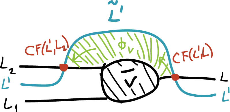
In the graded case there are some suspensions in the expression above - as in Lemma 4.4.1 - but we neglect them here. Similarly, there are certain signs in the matrix above that we again neglect as we work over $\mathbb{Z}_{2}$ . What matters here is that the upper left component of $D$ is a chain map $\tilde{\phi}_{V}:CF(L^{\prime},L)\to CF(L^{\prime},L_{2})$ . We put $\phi_{V}=[\tilde{\phi}_{V}]$ . We notice that as in the proof of Theorem 2.2.1 this map is uniquely defined up to chain homotopy and multiplication by a an element $T^{a}\in\mathcal{A}$ . In geometric terms, this map counts the Floer strips that project to the green strips in Figure 9.

The next step is to justify the commutativity of Diagram 20. For this verification we will identify geometrically the maps $\phi_{V}$ and $i_{1}$ and will relate them to the construction of $PSS^{\prime}$ . The geometric part of this argument consists in composing the two isotopic cobordisms $\overline{V}^{\prime}$ and $\overline{V}^{\prime\prime}$ from the Figures 7 and 8 with a cobordism of the form $\gamma\times L$ as in the Figure 10.

To be more precise, assume, without loss of generality, that the cylindrical positive end of both $\overline{V}^{\prime}$ and $\overline{V}^{\prime\prime}$ coincide with $[1,+\infty)\times\{2\}\times L$ . Assume also that the positive end of $\overline{V}$ coincides with $[1,+\infty)\times\{1\}\times L$ . Now take the curve $\gamma$ to be the graph of a function $g:[1,+\infty)\to\mathbb{R}$ so that $g$ is smooth, $g(t)=2$ for $t\in[1,2]\cup[4,+\infty)$ , $g$ attains its minimum at the point $3$ with minimal value $g(3)=-1$ and $3$ is the single critical point of $g$ in the interval $(2,4)$ . The curve $\gamma$ intersects (transversely) the curve $y=1$ in two points $P=(p,1)$ and $Q=(q,1)$ with $p<q$ . Finally, we put $\overline{W}^{\prime}=(\overline{V}^{\prime}\cap\pi^{-1}((-\infty,1]\times\mathbb{R}))\cup\gamma\times L$ and similarly $\overline{W}^{\prime\prime}=(\overline{V}^{\prime\prime}\cap\pi^{-1}(-\infty,1]\times\mathbb{R}))\cup\gamma\times L$ . Certainly, $\overline{W}^{\prime}$ is horizontally isotopic to $\overline{W}^{\prime\prime}$ (and both are horizontally isotopic with $\overline{V^{\prime}}$ and $\overline{V}^{\prime\prime}$ ). We will use the fact that the isotopy from $\overline{W}^{\prime}$ to $\overline{W}^{\prime\prime}$ may be assumed constant on $\pi^{-1}([1,+\infty)\times\mathbb{R})$ .

We use the two cobordisms $\overline{V}$ and $\overline{W}^{\prime}$ to deduce the commutativity of the following diagram:

(22)

where $j$ is the map induced in homology by the inclusion of the subcomplex of $CF(\overline{W}^{\prime},\overline{V})$ generated by the intersection points of $\overline{W}^{\prime}$ and $\overline{V}$ that project onto $Q$ ; $PSS^{\prime\prime}$ is a composition like $\eta\circ\overline{PSS}_{L_{1}}$ from Equation (21) only with $\overline{W}^{\prime}$ instead of $\overline{V}^{\prime}$ .

We now use the cobordisms $\overline{W}^{\prime\prime}$ and $\overline{V}$ . The fact that the horizontal isotopy from $\overline{W}^{\prime}$ to $\overline{W}^{\prime\prime}$ may be assumed constant $\pi^{-1}([1,+\infty)\times\mathbb{R})$ implies the commutativity of the triangle below up to multiplication with a term of the form $T^{a}$ :

(23)

Indeed, with the correct choice of perturbations and almost complex structure, the Floer complex $CF(\overline{W}^{\prime\prime},\overline{V})$ is of the form $(CF(L,L_{2})\oplus CF(L,L)[1]\oplus CF(L,L),D)$ where the differential $D$ is just the internal differential on both $CF(L,L_{2})$ and $CF(L,L)$ and on $CF(L,L)[1]$ (which is represented geometrically by the intersection points of $\overline{W}^{\prime\prime}$ and $\overline{V}$ that project on $P$ ) it has the form $D=d_{L}[1]+\phi_{V}-\textnormal{id}_{CF(L,L)}[-1]$ where $d_{L}$ is the differential on $CF(L,L)$ . The choice of isotopy shows that $j$ corresponds to the inclusion

CF(L,L)\to CF(L,L_{2})\oplus CF(L,L)[1]\oplus CF(L,L)

and this implies the commutativity of Diagram (23) up to multiplication by $T^{a}$ .

To summarize what was shown till now, we proved that Diagram (20) commutes and that $PSS$ and $PSS^{\prime}$ are isomorphisms. The next remark is that the morphism $\phi_{V}$ is a $QH(L;\mathcal{A})$ -module morphism. This an easy verification based on our definition of $\phi_{V}$ that we leave as exercise. As $QH(L)$ is a field this means that either $\phi_{V}$ is null or it is an injection. Thus, the same is true for $i_{1}$ and it is easy to see that a similar argument can be applied to the morphism $i_{2}$ from Diagram (19). The exactness of (19) together with the duality between the $i_{j}$ ’s and the $\eta_{r}$ ’s implies that one of the $i_{j}$ ’s has to vanish and the other is injective. We will assume that $i_{1}$ is injective and that $i_{2}$ vanishes. From Lemma 3.3.1 it is immediate to see that injectivity of $i_{1}$ with coefficients in $\mathcal{A}$ implies that the corresponding morphism $i_{1}^{\Lambda}:QH(L)\to QH(V,L_{1})$ is also injective. Similarly, the vanishing of $i_{2}$ with coefficients in $\mathcal{A}$ also implies the vanishing of $i_{2}$ over $\Lambda$ . To shorten notation we will not indicate the coefficients in the notation for these morphisms $i_{1}$ , $i_{2}$ , etc as long as there is no risk of confusion.

The first claim of the Theorem now follows easily. Indeed $i_{1}$ (now taken over $\Lambda$ ) factors:

QH(L)\to QH(V)\to QH(V,L_{1})

and thus $QH(L)\to QH(V)$ is injective. The rank inequality (2) follows immediately if we can show that for $I_{i}=Im(QH(L_{i})\to QH(V))$ and $I_{0}=Im(QH(L)\to QH(V))$ , we have $I_{1}\oplus I_{0}\subset I_{2}$ and $QH(L_{1})\to QH(V)$ is injective.

To do this we go back to the Diagram (19) and we start by noticing that the vanishing of $i_{2}$ implies that $k_{1}$ vanishes. This is seen as follows. First, by an argument similar to that applied to $i_{1}$ and $i_{2}$ we see that, over $\mathcal{A}$ , $k_{1}$ is a $QH(L_{1};\mathcal{A})$ -module map. Thus it suffices to show that $k_{1}([L_{1}])=0$ ( $[L_{1}]$ is the fundamental class and is the unit in $QH(L_{1};\mathcal{A})$ ). Secondly, by using explicitly the form of the pearl complexes associated to a function $f:V\to\mathbb{R}$ adapted to the exit region $L\cup L_{1}$ it is easy to see that $i_{2}([L])=k_{1}([L_{1}])$ and thus $k_{1}([L_{1}])=0$ . This means that $k_{1}$ vanishes over $\mathcal{A}$ . But this implies that it also vanishes over $\Lambda$ . Now $k_{1}$ and $s_{1}$ are dual so the vanishing of $k_{1}$ implies that of $s_{1}$ which means that $l_{1}:QH(L_{1})\to QH(V,L)$ is injective. But this implies that $QH(L_{1})\to QH(V)$ is injective.

We now show that $I_{0},I_{1}\subset I_{2}$ . This follows from the exact sequence:

\to QH(L_{2})\to QH(V)\to QH(V,L_{2})\to

combined with the fact that both maps $k_{1}:QH(L_{1})\to QH(V)\to QH(V,L_{2})$ and $i_{2}:QH(L)\to QH(V)\to QH(V,L_{2})$ vanish.

The last step is to show that $I_{0}\cap I_{1}=\{0\}$ . This follows form the exact sequence

\to QH(L_{1})\to QH(V)\to QH(V,L_{1})\to

together with the fact that the map $i_{1}:QH(L)\to QH(V)\to QH(V,L_{1})$ is injective. ∎

6. Examples

In this section we show Theorem 2.2.5. The examples presented here are based on the Lagrangian surgery construction as described for instance by Polterovich in [Pol]. These examples contrast with the rigidity results contained in the previous sections, in particular Theorems 2.2.1 and 2.2.2.

6.1. The trace of surgery as Lagrangian cobordism

The purpose here is to show that the trace of a Lagrangian surgery gives rise to a Lagrangian cobordism. As we shall see, this is a bit less obvious than one might first expect because Lagrangian cobordism is less flexible than Lagrangian isotopy.

We start with the local picture and fix the following two Lagrangians: $L_{1}=\mathbb{R}^{n}\subset\mathbb{C}^{n}$ and $L_{2}=i\mathbb{R}^{n}\subset\mathbb{C}^{n}$ .

We define a particular curve $H\subset\mathbb{C}$ , $H(t)=a(t)+ib(t)$ , $t\in\mathbb{R}$ , with the following properties (see also Figure 11):

i.

$H$ is smooth.
ii.

$(a(t),b(t))=(t,0)$ for $t\in(-\infty,-1]$ .
iii.

$(a(t),b(t))=(0,t)$ for $t\in[1,+\infty)$ .
iv.

$a^{\prime}(t),b^{\prime}(t)>0$ for $t\in(-1,1)$ .

Consider $L=H\cdot S^{n-1}\subset\mathbb{C}^{n}$ or more explicitly

L=\Bigl\{\bigl((a(t)+ib(t))x_{1},\ldots,(a(t)+ib(t))x_{n}\bigr)\mid t\in\mathbb{R},\,\sum x_{i}^{2}=1\Bigr\}\subset\mathbb{C}^{n}~.~

Lemma 6.1.1.

The submanifold $L\subset\mathbb{C}^{n}$ as defined above is Lagrangian and there is a Lagrangian cobordism $L\leadsto(L_{1},L_{2})$ .

By a slight abuse of notation (because we omit the handle from the notation) we will denote $L=L_{1}\#L_{2}$ .

Proof.

A straightforward calculation shows that $L\subset\mathbb{C}^{n}$ is Lagrangian (see e.g. [Pol]).

To construct the desired cobordism we now define

\widehat{H}=H\cdot S^{n}\subset\mathbb{C}^{n+1}~.~

Or more explicitly

\widehat{H}=\Bigl\{\bigl((a(t)+ib(t))x_{1},\ldots,(a(t)+ib(t))x_{n+1}\bigr)\mid t\in\mathbb{R},\,\sum x_{i}^{2}=1\Bigr\}~.~

A similar computation as before shows that $\widehat{H}$ is also Lagrangian.

We consider the projection $\pi:\mathbb{C}^{n+1}\to\mathbb{C}$ , $\pi(z_{1},\ldots z_{n+1})=z_{1}$ and we denote by $\widehat{\pi}$ its restriction to $\widehat{H}$ :

\widehat{\pi}((a(t)+ib(t))x_{1},\ldots,(a(t)+ib(t))x_{n+1})=(a(t)+ib(t))x_{1}~.~

Define $W=\widehat{\pi}^{-1}(S_{+})$ where $S_{+}=\{(x,y)\in\mathbb{R}^{2}\ |\ y\geq x\}$ , see Figure 12. (As usual, we identify $\mathbb{R}^{2}$ with $\mathbb{C}$ under $(x,y)\to x+iy$ .) A simple calculation shows that $W$ is a manifold with boundary.

Fix some $r<0$ and notice that if

\widehat{\pi}((a(t)+ib(t))(x_{1},\ldots,x_{n+1}))=(r,0)~,~

then $b(t)=0$ so that $t\leq-1$ and $a(t)=t$ . Moreover, $tx_{1}=r$ so that $\sum_{i=2}^{n+1}t^{2}x_{i}^{2}=t^{2}-r^{2}$ . Thus, for $r\leq-1$ , we have $\widehat{\pi}^{-1}(r,0)=(r,0)\times L_{1}\subset\mathbb{C}\times\mathbb{C}^{n}$ . Similarly, for $s\geq 1$ , $\widehat{\pi}^{-1}(0,s)=(0,s)\times L_{2}\subset\mathbb{C}\times\mathbb{C}^{n}$ . Also notice that $L=\widehat{\pi}^{-1}(0)$ .

We now only look to $W_{0}=W\cap\pi^{-1}([-2,0]\times[0,2])$ . It is not difficult to see that $W_{0}$ is a manifold with boundary and that $\partial W_{0}=\{(-2,0)\}\times L_{1}\cup\{(0,2)\}\times L_{2}\cup\{0,0\}\times L$ . We would like to be able to say that $W_{0}$ is a cobordism $W_{0}:L\leadsto(L_{1},L_{2})$ . For this however we still need to show that the $L$ -boundary component of $W_{0}$ can be continued to be cylindrical. We now describe explicitly this adjustment (the argument here is in fact quite general). Let $V_{L}\subset\mathbb{C}\times\mathbb{C}^{n}$ be the Lagrangian given by $V_{L}=\{(x,y)\in\mathbb{C}:x=-y\}\times L$ .

Put $L^{0}=\{(0,0)\}\times L$ . Note that $V_{L}\cap\pi^{-1}((0,0))=\widehat{H}\cap\pi^{-1}((0,0))=L^{0}$ . Fix a small neighborhood $U(L^{0})\subset\widehat{H}$ of $L^{0}\subset\widehat{H}$ and a Darboux-Weinstein neighborhood $\mathcal{N}\subset\mathbb{C}^{n+1}$ of $U(L^{0})$ and identify symplectically $\mathcal{N}$ with a tubular neighborhood of $U(L^{0})$ in $T^{*}U(L^{0})$ . Write $p:\mathcal{N}\to U(L^{0})$ for the projection corresponding via this identification to the projection in the cotangent bundle $T^{*}U(L^{0})\to U(L^{0})$ .

Note that at each point of $L^{0}$ , $V_{L}$ projects 1-1 on the tangent space of $\widehat{H}$ (via $p$ ). Thus reducing $U(L^{0})$ if necessary we can write $V_{L}\cap\mathcal{N}$ as the graph of a $1$ -form $\alpha$ on $U(L^{0})$ that vanishes on $L^{0}$ . Since $V_{L}$ is Lagrangian the form $\alpha$ is closed. As $U(L^{0})$ can be chosen so that it contracts to $L^{0}$ , we have $H^{1}(U(L^{0}),L^{0})=0$ hence $\alpha$ is exact. Let $f:U(L^{0})\to\mathbb{R}$ be so that $\alpha=df$ . Using a partition of unity construct $g:W\cup U(L^{0})\to\mathbb{R}$ so that it agrees with $f$ on $U(L^{0})\setminus W$ and vanishes outside a neighborhood of $U(L^{0})$ . Then the Lagrangian $W^{\prime}$ obtained by isotoping $W_{0}$ by the time-one Hamiltonian diffeomorphism induced by $X_{g}$ provides the cobordism desired between $L$ and $(L_{1},L_{2})$ - see also Figure 13. ∎

Remark 6.1.2.

i.

For further use, we notice that the homotopy type of the total space of the cobordism $W^{\prime}:L\leadsto L_{1}\#L_{2}$ constructed above coincides with that of the topological subspace of $M$ consisting of the union $L_{1}\cup L_{2}$ .
ii.

The construction described here also provides a cobordism $W^{\prime\prime}:(L_{2},L_{1})\to L_{2}\#L_{1}$ by simply using instead of $W$ the region $\widehat{\pi}^{-1}(S_{-})$ with

$S_{-}=\{(x,y)\in\mathbb{R}^{2}\ :\ y\leq x\}~.~$

Going from the local argument above to a global one is easy. Suppose that we have two Lagrangians $L^{\prime}$ and $L^{\prime\prime}$ that intersect transversely, possibly in more than a single point. At each intersection point we fix symplectic coordinates mapping (locally) $L^{\prime}$ to $\mathbb{R}^{n}\subset\mathbb{C}^{n}$ and mapping (again locally) $L^{\prime\prime}$ to $i\mathbb{R}^{n}\subset\mathbb{C}^{n}$ . We then apply the construction above at each of these intersection points. This produces a new Lagrangian submanifold $L^{\prime}\tilde{\#}L^{\prime\prime}$ as well as a cobordism $L^{\prime}\tilde{\#}L^{\prime\prime}\leadsto(L^{\prime},L^{\prime\prime})$ (we use $\tilde{\#}$ in the notation as $L^{\prime}\tilde{\#}L^{\prime\prime}$ is topologically not a connected sum if there are several intersection points). The homotopy type of $V$ coincides with that of the set $L^{\prime}\cup L^{\prime\prime}\subset M$ .

Remark 6.1.3.

a. The construction above can be used to produce examples of monotone cobordisms of the type $V:L\leadsto(L_{1},L_{2})$ . Indeed assume that $L_{1}$ and $L_{2}$ are uniformly monotone and intersect in a single point (for instance the longitude and latitude on a torus), then, as a consequence of a simple application of the Seifert Van Kampen Theorem, we have that $L=L_{1}\#L_{2}$ as well as the cobordism relating it to $(L_{1},L_{2})$ are also monotone with the same constants. The construction can be easily iterated to produce monotone cobordisms with arbitrarily many ends.

b. One can easily generalize the previous construction to a configuration of Lagrangian submanifolds $(L_{1},\ldots,L_{r})$ and the total surgery $L$ of the Lagrangians in the configuration. The result will be a Lagrangian cobordism $V:L\leadsto(L_{1},\ldots,L_{r})$ with one positive end and $r$ negative ends. Of course, monotonicity will in general not be preserved in this case. However, if the intersection diagram of the configuration is a tree, and if $(L_{1},\ldots,L_{r})$ are uniformly monotone, then the Lagrangian $L$ and the cobordism $V$ will be monotone too. An interesting example is when $(L_{1},\ldots,L_{r})$ is a configuration of Lagrangian spheres corresponding to a simple singularity. The relation between singularity theory and Fukaya categories has been extensively studied in recent years (see e.g. [Sei3]). Thus the constructions above (together with Theorem 2.2.1) suggests that the cobordism category is relevant in this study.

6.2. Cobordant Lagrangians that are not isotopic

In this subsection we will make use of the constructions described in §6.1 to prove Theorem 2.2.5 and thus construct an example of monotone cobordant connected Lagrangians that are not smoothly isotopic. We emphasize that while the two Lagrangians at the ends of the cobordism are exact, the minimal Maslov number of the cobordism $V$ between them is $N_{V}=1$ . We will also see that the two Lagrangians in question cannot be related by a monotone cobordism with minimal Maslov $\mu_{\textnormal{min}}\geq 2$ . A variety of other examples can be constructed following the same ideas.

We will start our construction in the ambient manifold $M=\mathbb{C}$ . We consider two circles $A=\{z\in\mathbb{C}\ :\ |z+1/2|=1\}$ and $B=\{x\in\mathbb{C}\ :\ |z-1/2|=1\}$ . We denote by $D(A)$ and $D(B)$ the two disks bounded by $A$ and $B$ respectively. We also consider two smooth curves in the plane $\mathbb{C}$ , $\gamma_{1}:[-1,1]\to\mathbb{C}$ and $\gamma_{2}:[-1,1]\to\mathbb{C}$ so that - see Figure 14:

i.

$\gamma_{1}(t)=t$ for $t\in[-1,-1/2]$
ii.

$\gamma_{1}(t)=1+(1-t)i$ for $t\in[1/2,1]$
iii.

$Re(\gamma_{1}(t))$ is strictly increasing for $t\in(-1/2,1/2-\epsilon)$ . $Im(\gamma_{1}(t))$ is strictly increasing for $t\in(-1/2,1/2-\epsilon)$ and strictly decreasing for $t\in(1/2-\epsilon,1/2)$ .
iv.

$\gamma_{2}(t)=-\gamma_{1}(t)$ for all $t\in[-1,1]$ .

We now consider the Lagrangians $A^{\prime}=\gamma_{2}\times A\subset\mathbb{C}\times M$ and $B^{\prime}=\gamma_{1}\times B\subset\mathbb{C}\times M$ . By performing surgery - as explained in §6.1 - at both intersection points $A\cap B$ we can extend the union of the two Lagrangians $A^{\prime}\cup B^{\prime}$ towards the positive end as well as towards the negative end as in the Figure 14 thus obtaining a cobordism $V:A\tilde{\#}B\leadsto B\tilde{\#}A$ .

Put $L=A\tilde{\#}B$ and $L^{\prime}=B\tilde{\#}A$ . With our choice of handles it is easy to see that $L$ and $L^{\prime}$ look as in Figure 15. Moreover, if the surgeries used in both intersection points of $A$ and $B$ use the same handle $H$ , then the area inside both circles is precisely $D(A)+D(B)-Area(D(A)\cap D(B))$ (the two handles can also be picked differently and this can modify the areas bounded by these two circles, thus producing a - non-monotone - cobordism relating non-Hamiltonian isotopic, connected Lagrangians).

It is easy to see that $V$ as constructed before is not orientable. Moreover, $V$ is also not monotone. However, it is possible to alter the ambient manifold and make the cobordism monotone in the following way. Instead of performing all the construction above in $M=\mathbb{C}$ we can as well do it in $M^{\prime}=\mathbb{C}\backslash\{P_{1},P_{2},P_{3}\}$ where the three points $P_{i}$ are such that $P_{1}\in D(A)\backslash D(B)$ , $P_{2}\in D(A)\cap D(B)$ and $P_{3}\in D(B)\backslash D(A)$ as in Figure 15. We will explicitly check monotonicity below. We notice for now that in $M^{\prime}$ , $L$ and $L^{\prime}$ are not even smoothly isotopic.

To verify that $V$ is monotone in $\mathbb{C}\times M^{\prime}$ we write $V=V_{+}\cup V_{-}$ , where $V_{+}=V\cap\pi^{-1}([0,+\infty)\times\mathbb{R})$ and $V_{-}=V\cap\pi^{-1}((-\infty,0]\times\mathbb{R})$ . Put $\widetilde{M^{\prime}}_{+}=([0,+\infty)\times\mathbb{R})\times M^{\prime}$ , $\widetilde{M^{\prime}}_{-}=((-\infty,0]\times\mathbb{R})\times M^{\prime}$ . Moreover, $V_{+}\cap V_{-}=\{P\}\times A\cup\{Q\}\times B$ , where $P=\gamma_{2}\cap i\mathbb{R}$ and $Q=\gamma_{1}\cap i\mathbb{R}$ . Each of $V_{+}$ and $V_{-}$ are homotopy equivalent to $A\cup B$ . In particular, $H_{2}(\widetilde{M^{\prime}}_{+},V_{+})=0$ and $H_{2}(\widetilde{M^{\prime}}_{-},V_{-})=0$ . This implies that $H_{2}(\mathbb{C}\times M^{\prime},V)=\mathbb{Z}\oplus\mathbb{Z}$ . There are two generators for this group each associated to one of the intersection points of $A$ and $B$ . Each of them is represented by a disk in $\mathbb{C}^{2}$ with boundary on $V$ that is given by a flat lift of the planar region bounded by the two curves $\gamma_{1}$ and $\gamma_{2}$ and the two planar projections of the handles at the ends. We orient these generators so as to be of positive area and we will now verify that they are both of Maslov index $1$ . The computation is the same for both generators and we fix just one of them, $D_{1}$ . Its boundary is a curve $\gamma:S^{1}\to\widetilde{M}=\mathbb{C}\times M$ whose projection onto $\mathbb{C}$ we denote still by $\gamma$ (this is, as mentioned before, the union of the two curves $\gamma_{1}$ and $\gamma_{2}$ and the two handles at the ends). We look at the tangent space $T_{x}V\subset T\widetilde{M}=\mathbb{C}\times\mathbb{C}$ for a point $x=\gamma(t)\in V$ . It is easy to see that this tangent space decomposes as:

T_{x}V=\mathbb{R}(\dot{\gamma}(t),0)+\mathbb{R}(0,N(t))

where $\dot{\gamma}$ is the tangent vector to $\gamma$ and $N(t)\in\mathbb{C}$ . We need to describe $N(t)$ more explicitly. For that we pick a parametrization for $\gamma$ - as described in Figure 14 - so that $\gamma:[0,8]\to\mathbb{C}$ , $\gamma(0)=P=\gamma(8)$ , $\gamma(4)=Q$ , $\gamma(t)=H(t-2)$ for $1\leq t\leq 3$ , $\gamma(t)=-H(t-6)$ for $5\leq t\leq 7$ . With this parametrization we can write $N(t)=H(t)\in\mathbb{C}$ for $1\leq t\leq 3$ ; $N(t)=iH(t)\in\mathbb{C}$ for $5\leq t\leq 7$ ; $N(t)$ is constant and tangent to $A$ in the intervals $[0,1]$ and $[7,8]$ (notice however that $N(8)\not=N(0)$ because $\gamma$ is orientation reversing) and $N(t)$ is constant and tangent to $B$ in the interval $[3,5]$ . The horizontal loop $\gamma$ is of Maslov index $2$ and from the formula above it follows that the contribution of $N(t)$ is $-1$ . Thus the total Maslov index of $D_{1}$ is $1$ .

By choosing the handles used for the intersection points appropriately we may arrange that these two generators have equal areas. Thus $V$ is monotone of minimal Maslov number $N_{V}=1$ .

It remains to show that $L$ and $L^{\prime}$ are not cobordant via a monotone cobordism with $\mu_{\textnormal{min}}\geq 2$ .¹¹ 1 This argument was suggested to us by the referee whom we would like to thank. Consider a positive ray $R^{+}$ starting at the point $P_{2}$ and having direction $i\mathbb{R}_{+}$ . While in the statements in our paper we always assume that the Lagrangians involved are compact, it is easy to see that all the techniques involved also apply to $R^{+}$ (alternatively the whole picture can be compactified - see Remark 6.2.1). Thus the Floer homologies $HF(R^{+},L)$ and $HF(R^{+},L^{\prime})$ are both defined. It is easy to see that they are not isomorphic as the first does not vanish (it is generated by the two intersection points between $R^{+}$ and $L$ ) and the second vanishes (as $R^{+}\cap L^{\prime}=0$ ). However, if $L$ and $L^{\prime}$ would be monotone cobordant via a cobordism with $\mu_{\textnormal{min}}\geq 2$ , then by Theorem 2.2.1 (in the case $k=1$ ) these two homologies should be isomorphic.

Remark 6.2.1.

It is possible to compactify $M^{\prime}$ to a closed surface (of high genus), while still keeping $V$ monotone. This can be done by enlarging the punctures around the points $P_{i}$ and adding appropriate handles. The ray $R^{+}$ will be compactified in this picture into a monotone circle.

7. Lagrangian cobordism as a category

The aim of this section is to explain how cobordism naturally organizes the Lagrangian submanifolds of a fixed symplectic manifold $(M,\omega)$ in a category and to describe a functor relating this cobordism category to the derived Fukaya category. We will then interpret Theorems 2.2.1, 2.2.2 and 2.2.3 from this perspective. In particular, a non elementary cobordism $V:L\leadsto(L_{1},\ldots L_{k})$ is viewed as a “splitting” of $L$ into the “pieces” $L_{1},\ldots,L_{k}$ .

As mentioned in the introduction an alternative categorical point of view on Lagrangian cobordism has been independently introduced by Nadler and Tanaka in [NT].

The data is organized in the following diagram

(24)

that will be explained below. The proof of the fact that $\widetilde{\mathcal{F}}$ and $\mathcal{F}$ above are functors is postponed to a forthcoming paper.

In the left corner of this Diagram 24 is the category $Cob^{d}_{0}(M)$ - the cobordism category of $M$ - formally described in §7.1. This is a geometric category with objects families of Lagrangians $(L_{1},\ldots,L_{k})$ , $L_{i}\in\mathcal{L}^{\ast}_{d}(M)$ (where $\mathcal{L}^{\ast}_{d}(M)$ is a class of Lagrangians that is also introduced in §7.1). The morphisms in this category correspond to (unions) of horizontal isotopy classes of cobordisms with a single positive end but possibly with many negative ones.

In the right corner in Diagram (24), $\mathcal{F}uk^{d}(M)$ , stands for the Fukaya category of $M$ with objects the Lagrangians in $\mathcal{L}^{\ast}_{d}(M)$ . The Floer constructions involved in defining the morphisms (and higher operations) in this $A_{\infty}$ -category are with $\mathbb{Z}_{2}$ replacing $\mathcal{A}$ (as explained in Remark 7.1.1; see also Remark 7.3.1 on why this change is required). $D\mathcal{F}uk^{d}(M)$ stands for the resulting derived Fukaya category of $M$ . The category $D\mathcal{F}uk^{d}(M)$ is triangulated and $\Sigma D\mathcal{F}uk^{d}(M)$ is the stabilization of $D\mathcal{F}uk^{d}(M)$ in the sense that the morphisms of $D\mathcal{F}uk^{d}(M)$ are enriched by those morphisms that shift “degree” (see §7.2).

Remark 7.0.1.

In the construction of $D\mathcal{F}uk^{d}(M)$ we do not complete with respect to idempotents (or split factors).

The category $T^{S}D\mathcal{F}uk^{d}(M)$ is obtained from the category $D\mathcal{F}uk^{d}(M)$ by a general construction (apparently new) that associates to any triangulated category $\mathcal{C}$ a new category $T^{S}\mathcal{C}$ - the category of (stable) triangular (or cone) resolutions over $\mathcal{C}$ . The morphisms sets $\hom(x,-)$ in this category parametrize the ways in which $x$ can be resolved by iterated exact triangles (or cone attachments). We present this construction below in §7.2. There is a canonical projection functor $\mathcal{P}:T^{S}\mathcal{C}\to\Sigma\mathcal{C}$ .

In view of the construction of $T^{S}(-)$ the objects in the category $T^{S}D\mathcal{F}uk^{d}(M)$ are also families $(L_{1},\ldots,L_{k})$ , $L_{i}\in\mathcal{L}^{\ast}_{d}(M)$ and, in fact, the functor $\widetilde{\mathcal{F}}$ is the identity on objects. Geometrically, the existence of $\widetilde{\mathcal{F}}$ is of interest because it associates to each morphism in $\mathcal{C}ob^{d}_{0}(M)$ and thus, to each cobordism $V:L\leadsto(L_{1},\ldots,L_{k})$ , an iterated decomposition of $L$ by exact triangles in $D\mathcal{F}uk^{d}(M)$ in terms of the $L_{i}$ ’s. In particular, one can deduce a variety of exact sequences relating the homologies of the ends as well as the higher structures. By §6.1 this applies, in particular, to surgery. This correspondence

cobordism\ \leftrightarrow\ triangular\ decomposition

is reminiscent of the statement in Theorem 2.2.1. Indeed, as we will see in §7.3 where we discuss the relations between this categorical point of view and our earlier results in the paper, this theorem is the basic stepping stone for the construction of $\widetilde{\mathcal{F}}$ .

7.1. The category $\mathcal{C}ob^{d}_{0}(M)$

The purpose of this subsection is to set up Lagrangian cobordism as a category. We first introduce an auxiliary category $\widetilde{{\mathcal{C}ob}^{d}}(M)$ , $d\in K$ . Its objects are families $(L_{1},L_{2},\ldots,L_{r})$ with $r\geq 1$ , $L_{i}\in\mathcal{L}_{d}(M)$ . (Recall that $\mathcal{L}_{d}(M)$ stands for the class of uniformly monotone Lagrangians $L$ with $d_{L}=d$ , and when $d\neq 0$ with the same monotonicity constant $\rho$ which is omitted from the notation.)

To describe the morphisms in this category we proceed in two steps. First, for any two horizontal isotopy classes of cobordisms $[V]$ and $[U]$ with $V:(L^{\prime}_{j})\leadsto(L_{i})$ (as in Definition 2.1.1) and $U:(K^{\prime}_{s})\leadsto(K_{r})$ we define the sum $[V]+[U]$ to be the horizontal isotopy class of a cobordism $W:(L^{\prime}_{j})+(K^{\prime}_{s})\leadsto(L_{i})+(K_{r})$ so that $W=V\coprod\widetilde{U}$ with $\widetilde{U}:(K^{\prime}_{s})\leadsto(K_{r})$ a cobordism horizontally isotopic to $U$ and so that $\widetilde{U}$ is disjoint from $V$ (to insure embeddedness we can not simply take $V$ and $U$ in the disjoint union.) Notice that the sum $[V]+[U]$ is not commutative.

The morphisms in $\widetilde{{\mathcal{C}ob}^{d}}(M)$ are now defined as follows. A morphism

[V]\in{\textnormal{Mor\/}}\bigl((L^{\prime}_{j})_{1\leq j\leq S},(L_{i})_{1\leq i\leq T}\bigr)

is a horizontal isotopy class that can be written as a sum $[V]=[V_{1}]+\cdots+[V_{S}]$ with each $V_{j}\in\mathcal{L}_{d}(\mathbb{C}\times M)$ a cobordism from the Lagrangian family formed by the single Lagrangian $L^{\prime}_{j}$ and a subfamily $(L_{r(j)},\ldots,L_{r(j)+s(j)})$ of the $(L_{i})$ ’s, and so that $r(j)+s(j)+1=r(j+1)$ . In other words, $V$ decomposes as a union of $V_{i}$ ’s each with a single positive end but with possibly many negative ones. We will often denote such a morphism by $V:(L^{\prime}_{j})\longrightarrow(L_{i})$ .

The composition of morphisms is induced by concatenation followed by a rescaling to reduce the “length” of the cobordism to the interval $[0,1]$ . It is an easy exercise to see that this is well defined precisely because our morphisms are (horizontal) isotopy classes of cobordisms and because morphisms are represented by sums of cobordisms with a single positive end - this is crucial to preserve monotonicity.

We will consider here the void set as a Lagrangian of arbitrary dimension. We now intend to factor both the objects and the morphisms in this category by equivalence relations that will transform this category in a strict monoidal one. For the objects the equivalence relation is induced by the relations

(25)

(L,\emptyset)\sim(\emptyset,L)\sim(L).

At the level of the morphisms a bit more care is needed. For each $L\in\mathcal{L}_{d}(M)$ we will define two particular cobordisms $\Phi_{L}:(\emptyset,L)\leadsto(L,\emptyset)$ and $\Psi_{L}:(L,\emptyset)\leadsto(\emptyset,L)$ as follows. Let $\gamma:[0,1]\to[0,1]$ be an increasing, surjective smooth function, strictly increasing on $(\epsilon,1-\epsilon)$ and with $\gamma^{\prime}(t)=0$ for $t\in[0,\epsilon]\cup[1-\epsilon,1]$ . We now let $\Phi(L)=graph(\gamma)\times L$ and $\Psi(L)=graph(1-\gamma)\times L$ . The equivalence relation for morphisms is now induced by the following two identifications:

(Eq 1)

For every cobordism $V$ we identify $V+\emptyset\sim\emptyset+V\sim V$ , where $\emptyset$ is the void cobordism between two void Lagrangians.
(Eq 2)

If $V:L\longrightarrow(L_{1},...,L_{i},\emptyset,L_{i+2},\ldots,L_{k})$ , then we identify $V\sim V^{\prime}\sim V^{\prime\prime}$ , where $V^{\prime}=\Phi_{L_{i+2}}\circ V$ , $V^{\prime\prime}=\Psi_{L_{i}}\circ V.$

We now construct the category $\mathcal{C}ob^{d}(M)$ . First we consider the full subcategory $\mathcal{S}\subset\widetilde{\mathcal{C}ob}^{d}(M)$ obtained by restricting the objects only to those families $(L_{1},\ldots,L_{k})$ with $L_{i}$ non-narrow for all $1\leq i\leq k$ (this is preferable because our functors ultimately make use of Floer homology and we need the quantum homology of each $L_{i}$ to be non trivial). Then $\mathcal{C}ob^{d}(M)$ is obtained by the quotient of the objects of $\mathcal{S}$ by the equivalence relation in (25) and the quotient of the morphisms of $\mathcal{S}$ by the equivalence relation in (Eq 1), (Eq 2).

This category is called the Lagrangian cobordism category of $M$ . As mentioned before, it is a strict monoidal category. To recapitulate, its objects are ordered families of Lagrangians $\in\mathcal{L}_{d}(M)$ and its morphisms:

[V]:(L^{\prime}_{j})\longrightarrow(L_{i})

can be represented by cobordisms $V\in\mathcal{L}_{d}(\mathbb{R}^{2}\times M)$ so that all $L_{i}$ ’s are non-void and all $L^{\prime}_{j}$ ’s are non-void except if there is just a single $L^{\prime}_{j}$ which can be void or there is just a single $L_{i}$ which can be void. Moreover, $V$ can be written as a disjoint union of cobordisms each with a single positive end.

It turns out that, for the the functorial picture in Diagram (24) to hold, an additional assumption is required on all the Lagrangians in our constructions, in addition to the monotonicity conditions discussed in §2.1.1. Every Lagrangian $L$ is required to satisfy

(26)

\textnormal{image\,}\bigl(\pi_{1}(L)\stackrel{{\scriptstyle i_{\ast}}}{{\longrightarrow}}\pi_{1}(M)\bigr)\ \ \mathrm{is\ torsion},

where $i_{\ast}$ is induced by the inclusion $L\subset M$ . An analogous constraint is imposed also to the Lagrangian cobordisms involved.

Remark 7.1.1.

Assuming the requirement (26), an observation due to Oh [Oh1] shows that all Floer complexes considered earlier in the paper are defined (at the chain level) with coefficients in the “polynomial” ring $\mathcal{A}^{0}=\Bigl\{\sum_{k=0}^{n}a_{k}T^{\lambda_{k}}\mid a_{k}\in K,\;n\in\mathbb{Z}\Bigr\}$ (i.e. those elements in $\mathcal{A}$ formed by finite sums). There is an obvious ring map $\mathcal{A}^{0}\to\mathbb{Z}_{2}$ obtained by sending $T\to 1$ and this allows to change the coefficients in all the structures described by specializing to $T=1$ . Clearly, all the results in this paper that have been established over $\mathcal{A}$ remain valid when working over $\mathbb{Z}_{2}$ using this change of coefficients, assuming of course that condition (26) is satisfied by all involved Lagrangians.

We denote by $\mathcal{L}^{\ast}_{d}(M)$ the Lagrangians in $\mathcal{L}_{d}(M)$ that are non-narrow and additionally satisfy (26). There is a subcategory of $\mathcal{C}ob^{d}(M)$ , that will be denoted by $\mathcal{C}ob^{d}_{0}(M)$ , whose objects consist of families of Lagrangians each one belonging to $\mathcal{L}^{\ast}_{d}(M)$ and whose morphisms are represented by Lagrangian cobordisms $V$ satisfying the analogous condition to (26), but in $\mathbb{R}^{2}\times M$ . This is again a strict monoidal category.

7.2. Cone decompositions over a triangulated category

In this subsection we will discuss a construction valid in any triangulated category. The purpose of the construction is to parametrize the various ways to decompose an object by iterated exact triangles.

Let $\mathcal{C}$ be a triangulated category. We recall [Wei] that this is an additive category together with a translation automorphism $T:\mathcal{C}\to\mathcal{C}$ and a class of triangles called exact triangles

X\stackrel{{\scriptstyle u}}{{\longrightarrow}}Y\stackrel{{\scriptstyle v}}{{\longrightarrow}}Z\stackrel{{\scriptstyle w}}{{\longrightarrow}}TX

that satisfy a number of axioms due to Verdier and to Puppe (see e.g. [Wei]).

A cone decomposition of length $k$ of an object $A\in\mathcal{C}$ is a sequence of exact triangles:

T^{-1}X_{i}\stackrel{{\scriptstyle u_{i}}}{{\longrightarrow}}Y_{i}\stackrel{{\scriptstyle v_{i}}}{{\longrightarrow}}Y_{i+1}\stackrel{{\scriptstyle w_{i}}}{{\longrightarrow}}X_{i}

with $1\leq i\leq k$ , $Y_{k+1}=A$ , $Y_{1}=0$ . (Note that $Y_{2}=X_{1}$ .) Thus $A$ is obtained in $k$ steps from $Y_{1}=0$ . To such a cone decomposition we associate the family $l(A)=(X_{1},X_{2},\dots,X_{k})$ and we call it the linearization of the cone decomposition. This definition is an abstractization of the familiar iterated cone construction in case $\mathcal{C}$ is the homotopy category of chain complexes. In that case $T$ is the shift functor $TX=X[-1]$ and the cone decomposition simply means that each chain complex $Y_{i+1}$ is obtained from $Y_{i}$ as the mapping cone of a morphism coming from some chain complex, in other words $Y_{i+1}=\textnormal{cone}(X_{i}[1]\stackrel{{\scriptstyle u_{i}}}{{\longrightarrow}}Y_{i})$ for every $i$ , and $Y_{1}=0$ , $Y_{k+1}=A$ .

We will now define a category $T^{S}\mathcal{C}$ . The construction of this category starts with the stabilization category of $\mathcal{C}$ , $\Sigma\mathcal{C}$ : $\Sigma\mathcal{C}$ has the same objects as $\mathcal{C}$ and the morphisms in $\Sigma\mathcal{C}$ from $a$ to $b\in\mathcal{O}b(\mathcal{C})$ are morphisms in $\mathcal{C}$ of the form $a\to T^{s}b$ for some integer $s$ . Next, the free monoidal isomorphism category $F^{\ast}\Sigma\mathcal{C}$ over $\Sigma\mathcal{C}$ has as objects finite families $(x_{1},\ldots,x_{k})$ where the $x_{i}$ ’s are objects in $\mathcal{C}$ . The monoidal addition, denoted by $+$ , is concatenation. The morphisms are corresponding families of isomorphisms in $\Sigma\mathcal{C}$ (thus this category differs from the free monoidal category over $\Sigma\mathcal{C}$ because that category has as morphisms families of morphisms and not only isomorphisms).

The category $T^{S}\mathcal{C}$ , called the category of (stable) triangle (or cone) resolutions over $\mathcal{C}$ is obtained from $F^{\ast}\Sigma\mathcal{C}$ by enriching the morphisms with the elements constructed as follows. Given $x\in\mathcal{O}b(\mathcal{C})$ and $(y_{1},\ldots,y_{q})\in\mathcal{O}b(F^{*}\Sigma\mathcal{C})$ a morphism $\Psi:x\longrightarrow(y_{1},\ldots,y_{q})$ is a triple $(\phi,a,\eta)$ , where $a\in\mathcal{O}b(\mathcal{C})$ , $\phi:x\to T^{s}a$ is an isomorphism for some index $s$ and $\eta$ is an equivalence class - in an obvious way - of a cone decomposition of the object $a$ with linearization $(T^{s_{1}}y_{1},T^{s_{2}}y_{2},\ldots,T^{s_{q-1}}y_{q-1},y_{q})$ for some family of indices $s_{1},\ldots,s_{q-1}$ . Below we will also sometimes use a shift index $s_{q}$ attached to the last element $y_{q}$ with the understanding that $s_{q}=0$ . Thus, not only $a$ admits a cone decomposition of length $q$ but such an equivalence class of decompositions is part of the data defining the morphism $\Psi$ .

We now define the morphisms between two general objects in $\mathcal{O}b(F^{\ast}\Sigma\mathcal{C})$ . A morphism

\Phi\in{\textnormal{Mor\/}}_{T^{S}\mathcal{C}}((x_{1},\ldots x_{m}),(y_{1},\ldots,y_{n}))

is a sum $\Phi=\Psi_{1}+\cdots+\Psi_{m}$ where $\Psi_{j}\in{\textnormal{Mor\/}}_{T^{S}\mathcal{C}}(x_{j},(y_{\alpha(j)},\ldots,y_{\alpha(j)+\nu(j)}))$ , and $\alpha(1)=1$ , $\alpha(j+1)=\alpha(j)+\nu(j)+1$ , $\alpha(m)+\nu(m)=n$ .

The composition of the morphisms in $T^{S}\mathcal{C}$ is not quite obvious (it uses the axioms of a triangulated category; it is described explicitly in [BC1]).

There is a projection functor

(27)

\mathcal{P}:T^{S}\mathcal{C}\longrightarrow\Sigma\mathcal{C}

that is defined by $\mathcal{P}(x_{1},\ldots x_{k})=x_{k}$ and whose value on morphisms is induced by associating to $\Phi\in{\textnormal{Mor\/}}_{T^{S}\mathcal{C}}(x,(x_{1},\ldots,x_{k}))$ , $\Phi=(\phi,a,\eta)$ , the composition:

\mathcal{P}(\Phi):x\stackrel{{\scriptstyle\phi}}{{\longrightarrow}}T^{s}a\stackrel{{\scriptstyle p}}{{\longrightarrow}}T^{s}x_{k}

with $p:a\to x_{k}$ defined by the last exact triangle in the cone decomposition $\eta$ of $a$ ,

T^{-1}x_{k}\longrightarrow a_{k}\longrightarrow a\stackrel{{\scriptstyle p}}{{\longrightarrow}}x_{k}~.~

7.3. Putting things together

With the definitions above we can now describe the functor $\widetilde{\mathcal{F}}$ .

The construction of $\widetilde{\mathcal{F}}$ is very simple at the level of objects:

\mathcal{O}b(\mathcal{C}ob^{d}_{0}(M))\ni(L_{1},\ldots,L_{k})\stackrel{{\scriptstyle\widetilde{\mathcal{F}}}}{{\longmapsto}}(L_{1},\ldots,L_{k})\in\mathcal{O}b(T^{S}D\mathcal{F}uk^{d}(M))~.~

To describe the functor $\widetilde{\mathcal{F}}$ on morphisms we first mention that this will be by definition a monoidal functor so that it is enough to describe $\widetilde{\mathcal{F}}(\Phi)$ where

\Phi\in{\textnormal{Mor\/}}_{\mathcal{C}ob^{d}_{0}(M)}(L,(L_{1},\ldots,L_{k}))~.~

Let

V:L\leadsto(L_{1},\ldots,L_{k})\ \textrm{with}\ \ [V]=\Phi~.~

The triangulated structure of $D\mathcal{F}uk^{d}(M)$ is induced from an $A_{\infty}$ - triangulated completion $\mathcal{F}uk^{d}(M)^{\wedge}$ of $\mathcal{F}uk^{d}(M)$ . As explained in [Sei3] there are multiple such completions but all are equivalent for our purposes. The precise version that we use here (see Remark 3.21 in [Sei3]) is obtained by first using the Yoneda embedding to view $\mathcal{F}uk^{d}(M)$ as a functor category over itself with values into chain complexes and then making use of the usual cone construction at the level of chain complexes to build a triangulated closure of the image of the embedding. The category $D\mathcal{F}uk^{d}(M)$ , has the same objects as $\mathcal{F}uk^{d}(M)^{\wedge}$ but its morphisms are obtained by applying the homology functor to the morphisms in $\mathcal{F}uk^{d}(M)^{\wedge}$ .

By rendering explicit the definitions of the various categories involved we see that to construct $\widetilde{\mathcal{F}}(\Phi)$ we need to associate to each $N\in\mathcal{L}_{d}^{\ast}(M)$ a sequence of chain complexes $Z^{N}_{i}$ , $1\leq i\leq k+1$ , with $Z_{1}^{N}=0$ , and chain morphisms $u_{i}:CF(N,L_{i})\longrightarrow Z_{i}^{N}$ so that

(28)

Z_{i+1}^{N}=\textnormal{cone}(CF(N,L_{i})\stackrel{{\scriptstyle u_{i}}}{{\longrightarrow}}Z^{N}_{i}),\;\;\forall\,1\leq i\leq k,

as well as a chain homotopy equivalence $\phi_{V}^{N}:CF(N,L)\longrightarrow Z^{N}_{k+1}$ (we again neglect the grading here). Moreover, this association is supposed to be functorial in $N$ , there should be a compatibility with all the higher structures of an $A_{\infty}$ -category as well as with the composition of cobordisms.

While these functoriality verifications are postponed to a later publication we remark that the existence of the exact sequences in (28) is precisely the statement of Theorem 2.2.1 !

Remark 7.3.1.

Working over $\mathbb{Z}_{2}$ instead of $\mathcal{A}$ (and thus the requirement (26)) is crucial here because the maps $u_{i}$ , $\phi^{N}_{V}$ above should not depend on any additional choices. This is true over $\mathbb{Z}_{2}$ but only true up to multiplication with some $T^{a}\in\mathcal{A}$ if working over $\mathcal{A}$ .

Finally, from the point of view described here, the Theorems 2.2.2 and 2.2.3 can be viewed as exhibiting algebraic obstructions to the existence of morphisms in $\mathcal{C}ob^{d}(M)$ .

References

[Abo] M. Abouzaid. Homogeneous coordinate rings and mirror symmetry for toric varieties. Geom. Topol., 10:1097–1157 (electronic), 2006.
[Alb] P. Albers. A Lagrangian Piunikhin-Salamon-Schwarz morphism and two comparison homomorphisms in Floer homology. Int. Math. Res. Not. IMRN, (4):Art. ID rnm134, 56, 2008.
[ALP] M. Audin, F. Lalonde, and L. Polterovich. Symplectic rigidity: Lagrangian submanifolds. In M. Audin and J. Lafontaine, editors, Holomorphic curves in symplectic geometry, volume 117 of Progr. Math., pages 271–321, Basel, 1994. Birkhäuser Verlag.
[Arn1] V. Arnol^′d. Lagrange and Legendre cobordisms. I. Funktsional. Anal. i Prilozhen., 14(3):1–13, 96, 1980.
[Arn2] V. Arnol^′d. Lagrange and Legendre cobordisms. II. Funktsional. Anal. i Prilozhen., 14(4):8–17, 95, 1980.
[Aud] M. Audin. Quelques calculs en cobordisme lagrangien. Ann. Inst. Fourier (Grenoble), 35(3):159–194, 1985.
[Aur] D. Auroux. Fukaya categories of symmetric products and bordered Heegaard-Floer homology. J. Gökova Geom. Topol. GGT, 4:1–54, 2010.
[BC1] P. Biran and O. Cornea. Lagrangian cobordism II. In preparation.
[BC2] P. Biran and O. Cornea. Quantum structures for Lagrangian submanifolds. Preprint (2007). Can be found at http://arxiv.org/pdf/0708.4221.
[BC3] P. Biran and O. Cornea. A Lagrangian quantum homology. In New perspectives and challenges in symplectic field theory, volume 49 of CRM Proc. Lecture Notes, pages 1–44. Amer. Math. Soc., Providence, RI, 2009.
[BC4] P. Biran and O. Cornea. Rigidity and uniruling for Lagrangian submanifolds. Geom. Topol., 13(5):2881–2989, 2009.
[BC5] P. Biran and O. Cornea. Lagrangian topology and enumerative geometry. Geometry. Topol., 16:963–1052, 2012.
[BH] R. Brown and P. Higgins. On the connection between the second relative homotopy groups of some related spaces. Proc. London Math. Soc. (3), 36(2):193–212, 1978.
[Che] Y. Chekanov. Lagrangian embeddings and Lagrangian cobordism. In Topics in singularity theory, volume 180 of Amer. Math. Soc. Transl. Ser. 2, pages 13–23. Amer. Math. Soc., Providence, RI, 1997.
[Eli] Y. Eliashberg. Cobordisme des solutions de relations différentielles. In South Rhone seminar on geometry, I (Lyon, 1983), Travaux en Cours, pages 17–31. Hermann, Paris, 1984.
[FHS] A. Floer, H. Hofer, and D. Salamon. Transversality in elliptic Morse theory for the symplectic action. Duke Math. J., 80(1):251–292, 1995.
[FOOO1] K. Fukaya, Y.-G. Oh, H. Ohta, and K. Ono. Lagrangian intersection Floer theory - anomaly and obstruction, chapter 10. Preprint, can be found at http://www.math.kyoto-u.ac.jp/~fukaya/Chapter10071117.pdf.
[FOOO2] K. Fukaya, Y.-G. Oh, H. Ohta, and K. Ono. Lagrangian intersection Floer theory: anomaly and obstruction. Part I, volume 46 of AMS/IP Studies in Advanced Mathematics. American Mathematical Society, Providence, RI, 2009.
[FOOO3] K. Fukaya, Y.-G. Oh, H. Ohta, and K. Ono. Lagrangian intersection Floer theory: anomaly and obstruction. Part II, volume 46 of AMS/IP Studies in Advanced Mathematics. American Mathematical Society, Providence, RI, 2009.
[IP] E.N. Ionel and T.H. Parker. Relative Gromov-Witten invariants. Annals of Math., 157:45–96, 2003.
[NT] D. Nadler and H.L. Tanaka. A stable infinity-category of lagrangian cobordisms. Preprint (2011). Can be found at http://arxiv.org/pdf/1109.4835v1.
[Oh1] Y.-G. Oh. Floer cohomology of Lagrangian intersections and pseudo-holomorphic disks. I. Comm. Pure Appl. Math., 46(7):949–993, 1993.
[Oh2] Y.-G. Oh. Addendum to: ”Floer cohomology of Lagrangian intersections and pseudo-holomorphic disks. I.” [Comm. Pure Appl. Math. 46 (1993), no. 7, 949–993]. Comm. Pure Appl. Math., 48(11):1299–1302, 1995.
[Oh3] Y.-G. Oh. Floer cohomology, spectral sequences, and the Maslov class of Lagrangian embeddings. Internat. Math. Res. Notices, 1996(7):305–346, 1996.
[Oh4] Y.-G. Oh. Relative floer and quantum cohomology and the symplectic topology of lagrangian submanifolds. In C. B. Thomas, editor, Contact and symplectic geometry, volume 8 of Publications of the Newton Institute, pages 201–267. Cambridge Univ. Press, Cambridge, 1996.
[Oh5] Y.-G. Oh. Floer homology and its continuity for non-compact Lagrangian submanifolds. Turkish J. Math., 25(1):103–124, 2001.
[Pol] L. Polterovich. The surgery of Lagrange submanifolds. Geom. Funct. Anal., 1(2):198–210, 1991.
[Sei1] P. Seidel. Graded Lagrangian submanifolds. Bull. Soc. Math. France, 128(1):103–149, 2000.
[Sei2] P. Seidel. A long exact sequence for symplectic floer cohomology. Topology, 42(5):1003–1063, 2003.
[Sei3] P. Seidel. Fukaya categories and Picard-Lefschetz theory. Zurich Lectures in Advanced Mathematics. European Mathematical Society (EMS), Zürich, 2008.
[Wei] A. Weibel. An introduction to homological algebra, volume 38 of Cambridge Studies in Advanced Mathematics. Cambridge University Press, Cambridge, 1994.

Lagrangian cobordism I.Thanks: The second author was supported by an NSERC Discovery grant and a FQRNT Group Research grant

1. Introduction

Acknowledgments

2. Main results

2.1. Setting.

2.1.1. Monotonicity

2.1.2. Cobordism: main definition.

Definition 2.1.1.

2.2. Statement of the results.

2.2.1. Floer homology exact sequences.

Theorem 2.2.1.

2.2.2. Quantum homology restrictions

Theorem 2.2.2.

Theorem 2.2.3.

Remark 2.2.4.

2.2.3. Examples

Theorem 2.2.5.

2.3. Comments on the definition of cobordism and some constructions

Remark 2.3.1.

3. A quick review of Lagrangian Floer theory

3.1. Lagrangian Floer homology

Remark 3.1.1.

Remarks 3.1.2.

3.2. Moving boundary conditions

Remark 3.2.1.

3.3. The pearl complex and Lagrangian quantum homology

Lemma 3.3.1.

Proof.

3.3.1. The PSS isomorphism

3.4. Products and other structures

4. Floer homology and the proof of Theorem 2.2.1

4.1. Lagrangian submanifolds with cylindrical ends

Definition 4.1.1.

Definition 4.1.2 (Horizontal isotopies).

4.2. Compactness

Lemma 4.2.1.

Proof.

Remark 4.2.2.

4.3. Definition of Floer homology for Lagrangians with cylindrical ends

Proposition 4.3.1.

Proof of Proposition 4.3.1.

4.4. Non-existence of certain holomorphic strips and the proof of Theorem 2.2.1

Lemma 4.4.1.

Remark 4.4.2.

Proof of Lemma 4.4.1.

Remark 4.4.3.

Remark 4.4.4.

5. Quantum homology and the proofs of Theorems 2.2.2 and 2.2.3

5.1. Quantum homology for Lagrangians with cylindrical ends

Proposition 5.1.1.

Proof.

Lemma 5.1.2.

Proof.

Remark 5.1.3.

5.2. The PSS isomorphism for Lagrangians with cylindrical ends

Proposition 5.2.1.

Proof.

Lemma 5.2.2.

Proof of Lemma 5.2.2.

5.3. Proof of Theorem 2.2.2

Proof.

Remark 5.3.1.

5.4. Proof of Theorem 2.2.3

Proof.

6. Examples

6.1. The trace of surgery as Lagrangian cobordism

Lemma 6.1.1.

Proof.

Remark 6.1.2.

Remark 6.1.3.

6.2. Cobordant Lagrangians that are not isotopic

Remark 6.2.1.

7. Lagrangian cobordism as a category

Remark 7.0.1.

7.1. The category 𝒞​o​b0d​(M)\mathcal{C}ob^{d}_{0}(M)

Remark 7.1.1.

7.2. Cone decompositions over a triangulated category

7.3. Putting things together

Remark 7.3.1.

References

7.1. The category $\mathcal{C}ob^{d}_{0}(M)$