Lepton electric and magnetic dipole moments via lepton flavor violating spin-1 unparticle interactions

The Feynman diagram contributing to the electromagnetic vertex is shown in Fig. 1. From Eqs. (2) and (3) we obtain the interactions of the spin-1 unparticle with both vector and axial-vector LFV couplings. We will use Feynman parameters for the calculation and the spectral form for the unparticle propagator will be considered:

After the momentum space integration is worked out, we will proceed with the spectral integral.

After some lengthy algebra we arrive at the following results. The MDM of the lepton $j$ due to spin-1 unparticle can be written as

where the $F_{J}$ functions can be written as

with $\sqrt{r_{i}}=m_{j}/m_{i}$ and

also $f_{A}(z,{{d_{\mathcal{U}}}})=f_{V}(-z,{{d_{\mathcal{U}}}})$. We note that there is a flip in the sign of the vector and axial-vector couplings.

For our analysis below, we will also need the contribution to $a_{\mu}$ from a spin-0 unparticle with both scalar and pseudoscalar LFV couplings. We obtain a similar result as that given by Eqs. (16) and (17), with $J$ running over $S$ and $P$, while the $f_{S}$ function is

and $f_{P}(z,{{d_{\mathcal{U}}}})=f_{S}(-z,{{d_{\mathcal{U}}}})$. These results coincide with those presented in [23] and serve as a cross-check for our calculation method.

We would also like to note that in the case of diagonal unparticle couplings, we obtain for the spin-0 and spin-1 unparticle contributions to $a_{\ell}$:

where $\lambda^{\ell}_{J}=\lambda_{J}^{\ell\ell}$ stands for the diagonal unparticle couplings. This result agrees with the result presented in [22] for the electron MDM.

As far as the lepton EDM is concerned, we will consider the contribution from both spin-0 and spin-1 unparticles. The EDM of fermion $j$, which can only arise if both $\lambda_{V}^{ij}$ and $\lambda_{A}^{ij}$ ($\lambda_{S}^{ij}$ and $\lambda_{P}^{ij}$) are nonzero and have an imaginary phase, is given by

where $(J,K)$ runs over $(V,A)$ and $(S,P)$. The $G_{(J,K)}$ functions are defined as

with

In the limit of a heavy internal lepton, $m_{j}\ll m_{i}$, the integration can be dealt with and we obtain

These expressions can be useful for the muon and tau loop contributions to the electron EDM and the tau loop contribution to the muon EDM.

A comprehensive analysis of the spin-1 unparticle contribution to the muon MDM would require to deal with several free parameters: six coupling constants, the unparticle scale and the unparticle operator dimension. We will take another approach instead and consider some particular scenarios of LFV together with the hypothesis that there is no large cancellation between different unparticle contributions. First of all, we will assume that there is a hierarchy in the LFV unparticle couplings as it is assumed in other models of LFV, i.e., $|\lambda^{e\mu}|<|\lambda^{e\tau}|<|\lambda^{\mu\tau}|\ll\lambda^{ii}$ for all the unparticle couplings. Since experimental data strongly constrains LFV between the muon and the electron, we will concentrate on the scenario where LFV transitions are dominated by the couplings of spin-1 unparticles with the tau and muon leptons. More specifically, we will focus on the three following scenarios:

• A-

  Vector and axial-vector LFV couplings of similar size.

• B-

  Vector-dominated LFV couplings.

• C-

  Axial-vector-dominated LFV couplings.

To discuss these scenarios we first evaluate numerically each term, $F_{J}(m_{i},{d_{\mathcal{U}}})$, of the sum of Eq. (16). The results are shown in Fig. 2 as functions of the dimension ${d_{\mathcal{U}}}$ and for $\Lambda_{\mathcal{U}}=1$ TeV. We do not show the contributions due to the electron loop as we assumed that the LFV couplings involving the electron are subdominant. While the contributions from vector couplings are positive, the axial-vector contributions are negative. We also note that $F_{A}(m_{i},{d_{\mathcal{U}}})\simeq-F_{V}(m_{i},{d_{\mathcal{U}}})$ and so the vector and axial-vector contributions can largely cancel out. This effect is more evident for the contributions of the tau lepton. Furthermore, the contributions from axial-vector couplings are larger in magnitude than the vector contributions, with the largest contribution arising from the muon loop. It means that as long the vector and axial-vector unparticle couplings were of similar order of magnitude (scenario A) the total contribution to the muon MDM could be negative. This is a scenario disfavored by the current experimental data, which requires a positive contribution to $a_{\mu}^{\mathcal{U}}$ from new physics. The situation is rather similar for the scalar and pseudoscalar contributions, which for comparison purposes are shown in Fig. 3, although in this case the scalar contributions are slightly larger in magnitude than the axial-vector contributions. If all the unparticle couplings were of similar size, the unparticle contribution to $a_{\mu}^{\mathcal{U}}$ could be negative as the axial-vector plus pseudoscalar contributions could be dominant. However, even if all the unparticle couplings were large, the total contribution to $a_{\mu}$ could still be positive by a sort of fine-tuning. We consider the scenario in which the axial-vector couplings are negligible in comparison to the vector couplings (scenario B), such that the total contribution to $a_{\mu}^{\mathcal{U}}$ is positive. Below we will analyze the possible constraints on vector unparticle couplings under this assumption.

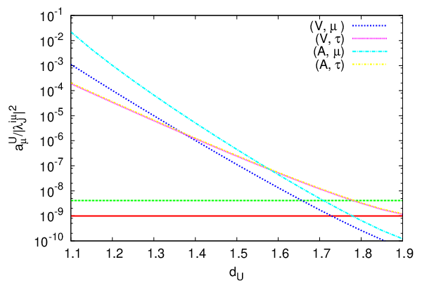
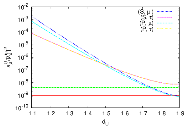
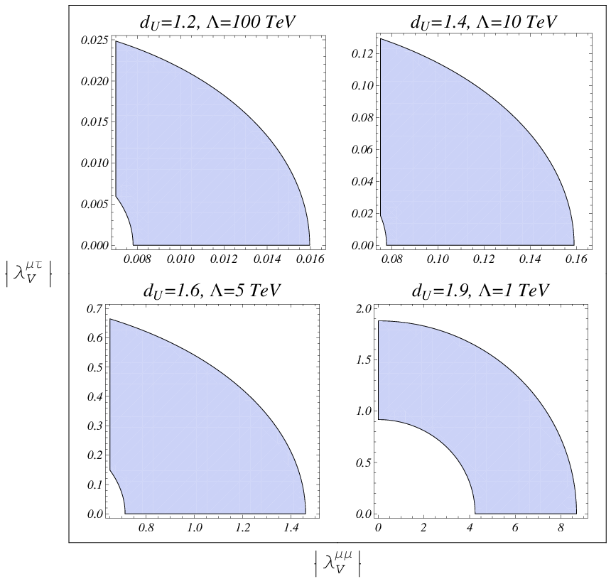
If the current discrepancy between the theoretical SM prediction and the experimental value of the muon MDM is assumed to be due entirely to unparticle interactions, the allowed limits with 95 % C.L. for this class of contributions are $98.2\times 10^{-11}\leq a_{\mu}^{\mathcal{U}}\leq 411.8\times 10^{-11}$. We have found the allowed area on the $|\lambda_{V}^{\tau\mu}|$ vs $|\lambda_{V}^{\mu\mu}|$ plane, which is shown in Fig. 4, for several values of $\Lambda_{\mathcal{U}}$ and ${d_{\mathcal{U}}}$ that are consistent with the bounds obtained for the scale $\Lambda_{\mathcal{U}}$ from mono-photon production at LEP [11] (see Table 1). As inferred from Fig. 4, the experimental data allow a magnitude of the vector couplings as large as unity for ${d_{\mathcal{U}}}\simeq 2$ and $\Lambda_{\mathcal{U}}=1$ TeV, whereas the most strong constraints are obtained for ${d_{\mathcal{U}}}$ close to unity. In general the limits on $|\lambda^{\mu\tau}_{V}|$ are slightly stronger than the limits on $|\lambda^{\mu\mu}_{V}|$, which is in agreement with our assumption. We also note that the bounds on the vector and axial-vector unparticle couplings are of similar order of magnitude than the bounds on the scalar and pseudoscalar unparticle couplings, as shown in Fig. 5. To obtain that plot we have assumed that the dominant contribution to the muon MDM arise from a spin-0 unparticle.

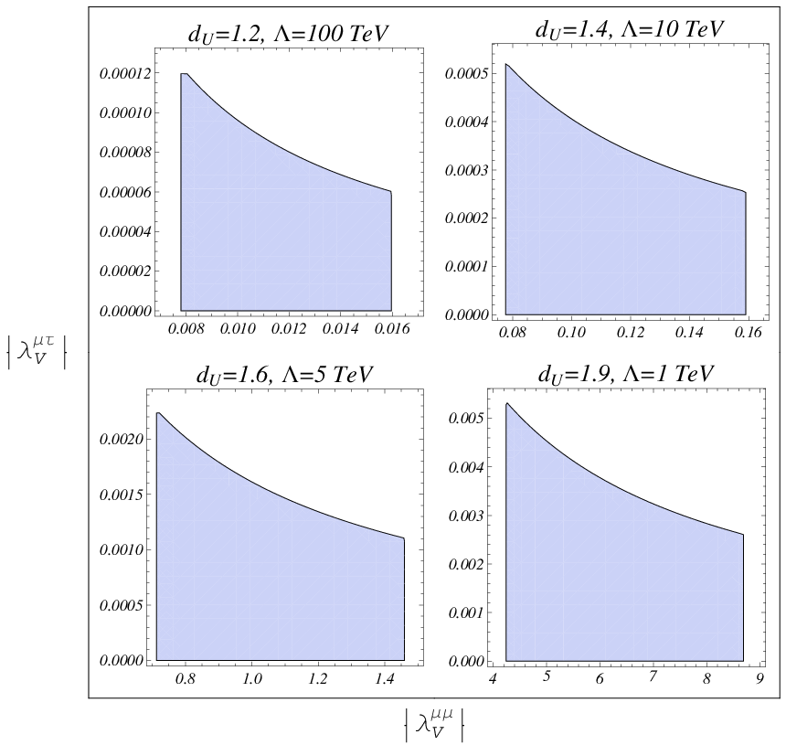
It has been long known that LFV couplings can also be constrained from the experimental bounds on the tree-level induced decays $\ell_{i}^{-}\to\ell_{j}^{-}\ell_{k}^{-}\ell_{k}^{+}$. We will examine the bounds obtained from the $\tau\to 3\mu$ decay, which involves the $\lambda_{V}^{\mu\mu}$ and $\lambda_{V}^{\tau\mu}$ couplings. The calculation for the $\ell_{i}^{-}\to\ell_{j}^{-}\ell_{k}^{-}\ell_{k}^{+}$ decay width was already presented in [19] for the scalar unparticle contribution. We have calculated the contribution from vector unparticles and the result is presented in the Appendix A. Let us consider the scenario we are working in, and neglect the axial-vector contributions. With these assumptions we can write for the $\tau\to 3\mu$ branching ratio:

with $\tau_{\tau}$ the tau mean life. The right-hand side of the inequality is the experimental constraint [33] and the $\eta_{1}$ function is defined in Appendix A.

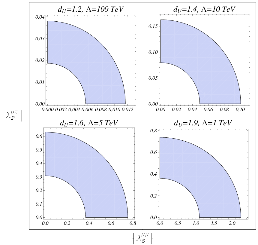
Eqs. (16) and (27) can serve to further constrain the allowed values of the coupling constants. We show in Fig. 6 the allowed area obtained after numerical evaluation of Eq. (27) for several values of $\Lambda_{\mathcal{U}}$ and ${d_{\mathcal{U}}}$. We observe that the $\tau\to 3\mu$ decay constrains considerably the size of the $\lambda_{V}^{\mu\tau}$ parameter, whose allowed value is extremely small for ${d_{\mathcal{U}}}$ close to unity, where the $\lambda_{V}^{\mu\mu}$ allowed values are considerably larger. There is also an allowed area in which the opposite is true ($|\lambda_{V}^{\mu\tau}|\gg|\lambda_{V}^{\mu\mu}|$), but we will not consider it as conflicts with our previous assumptions. For comparison purposes, we also have obtained the allowed area on the $|\lambda^{\mu\tau}_{S}|$ vs $|\lambda^{\mu\mu}_{S}|$ plane when it is considered that LFV scalar unparticle couplings give the main contributions to the muon MDM and the $\tau\to 3\mu$ decay. The results are shown in Fig. 7 for several values of $\Lambda_{\mathcal{U}}$ and ${d_{\mathcal{U}}}$. We observe that the allowed size of the scalar unparticle couplings is of similar order of magnitude than for the vector unparticle couplings.

We also analyzed the possible constraints obtained from the $\tau\to\mu\gamma$ decay. It involves the $\lambda_{V}^{\mu\tau}$, $\lambda_{V}^{\mu\mu}$ and $\lambda_{V}^{e\tau}$ couplings. We find that the respective constraints are less stringent than the ones obtained in Fig. 6, so we will not consider this decay mode.

In order to have a nonzero EDM, both kind of unparticle couplings, vector-axial or scalar-pseudoscalar, must be nonzero. Also, an imaginary phase is required. We will try to get an estimate of the order of magnitude for the electron and muon EDMs induced by unparticles. Apart from the magnitude of the $|\lambda_{V,A}^{ij}|$ and $|\lambda_{S,P}^{ij}|$ parameters, the EDM depends on the associated CP-violating phases, so its analysis is even more complicated. The most general form for the unparticle couplings is $\lambda_{J}^{ij}=|\lambda_{J}^{ij}|\exp(-i\theta_{J}^{ij})$, where $\theta_{J}^{ij}=-\theta_{J}^{ji}$ is a CP-violating phase. Therefore ${\rm Im}(\lambda_{J}^{ij}{\lambda_{K}^{*ij}})=|\lambda_{J}^{ij}||\lambda_{K}^{ij}|\sin\delta\theta_{(J,K)}^{ij}$, with $\delta\theta_{(J,K)}^{ij}=\theta_{J}^{ij}-\theta_{K}^{ij}$ the relative phase between $J$ and $K$ couplings. Depending on the relative sign of the CP violating phases, $\delta\theta_{(V,A)}^{ij}$ and $\delta\theta_{(S,P)}^{ij}$, the partial contributions can add coherently or destructively. We will content ourselves with considering a somewhat restrictive scenario, which will allows us to get an estimate of the order of magnitude of the EDM. First of all, as was the case for the muon MDM, we will assume that there is no large cancellation between different contributions to the EDM, so we can analyze each contribution separately. Also, to be consistent with the previous discussion, we will assume the following hierarchy $|\lambda_{V,S}^{\mu\tau}|\gg|\lambda_{V,S}^{\mu e}|$ and $|\lambda_{V,S}^{e\tau}|\gg|\lambda_{V,S}^{e\mu}|$. It means that the EDM would be entirely driven by the tau loop contributions. In view of this scenario, we numerically evaluate the tau loop contributions to the $G_{(J,K)}$ functions of Eq. (21). The results are shown in Fig. 8. We observe that the contribution from the tau loop to the electron and muon EDMs are indistinguishable, which means that the EDM is entirely controlled by the magnitude of the couplings constants and the imaginary phases. For this calculation we used the approximate formulas given by Eqs. (25) and (26), and made a cross-check with the exact calculation obtained by numerical integration of Eqs. (23) and (24).

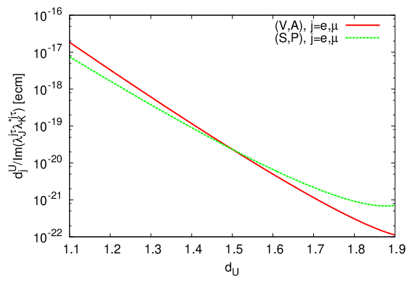
We now consider the constraints on the coupling constants obtained above to estimate the muon EDM in our working scenario. Both $(V,A)$ and $(S,P)$ contributions are of the order of $10^{-17}$ e-cm for ${d_{\mathcal{U}}}\simeq 1.1$ and $10̣^{-21}$ e-cm for ${d_{\mathcal{U}}}\simeq 1.6$. We will consider the case in which the $(V,A)$ coupling prevails over the $(S,P)$ couplings. The allowed magnitude of the $|\lambda_{V}^{\mu\tau}|$ parameter is of the order of $10^{-5}$ for ${d_{\mathcal{U}}}=1.1$ and $10^{-3}$ for ${d_{\mathcal{U}}}=1.6$. A good assumption for the $|\lambda_{A}^{\mu\tau}|$ coupling is that its magnitude is about one or two orders of magnitude below $|\lambda_{V}^{\mu\tau}|$. This would not spoil the bounds we obtained above. Therefore the muon EDM is about $|d_{\mu}^{\mathcal{U}}|\simeq|\sin\delta_{(V,A)}^{\mu\tau}|\times 10^{-30}$ e-cm for ${d_{\mathcal{U}}}\simeq 1.1$, whereas $|d_{\mu}^{\mathcal{U}}|\simeq|\sin\delta_{(V,A)}^{\mu\tau}|\times 10^{-29}$ e-cm for ${d_{\mathcal{U}}}\simeq 1.6$. These results are well below from the experimental limit on the muon EDM as the imaginary phase is expected to be very small. The magnitude of the coupling constants for LFV transitions involving the electron are expected to be more suppressed as long as the hierarchy discussed above is respected. Then we can estimate that the electron EDM induced by vector unparticles is well below the $10^{-30}$ e-cm level and far from the experimental measurement. Moreover, since the constraints on LFV spin-0 and spin-1 unparticle couplings are similar, the contributions to the muon and electron EDMs from both spin-0 and spin-1 unparticles are expected to be of similar size. Even if all different unparticle contributions add coherently, it is hard to expect a large size of the electron and muon EDMs due to unparticles.

References

- [1] T. Banks and A. Zaks, Nucl. Phys. B 196, 189 (1982).
- [2] H. Georgi, Phys. Rev. Lett. 98, 221601 (2007) [arXiv:hep-ph/0703260].
- [3] H. Georgi, Phys. Lett. B 650, 275 (2007) [arXiv:0704.2457 [hep-ph]].
- [4] G. Mack, Commun. Math. Phys. 55, 1 (1977).
- [5] Y. Nakayama, Phys. Rev. D 76, 105009 (2007) [arXiv:0707.2451 [hep-ph]].
- [6] B. Grinstein, K. A. Intriligator and I. Z. Rothstein, Phys. Lett. B 662, 367 (2008) [arXiv:0801.1140 [hep-ph]].
- [7] M. Luo and G. Zhu, Phys. Lett. B 659, 341 (2008) [arXiv:0704.3532 [hep-ph]].
- [8] S. L. Chen and X. G. He, Phys. Rev. D 76, 091702 (2007) [arXiv:0705.3946 [hep-ph]].
- [9] Y. Liao, Phys. Lett. B 665, 356 (2008) [arXiv:0804.0752 [hep-ph]].
- [10] K. Cheung, W. Y. Keung and T. C. Yuan, Phys. Rev. Lett. 99, 051803 (2007) [arXiv:0704.2588 [hep-ph]].
- [11] K. Cheung, W. Y. Keung and T. C. Yuan, Phys. Rev. D 76, 055003 (2007) [arXiv:0706.3155 [hep-ph]].
- [12] P. Mathews and V. Ravindran, Phys. Lett. B 657, 198 (2007) [arXiv:0705.4599 [hep-ph]].
- [13] M. C. Kumar, P. Mathews, V. Ravindran and A. Tripathi, Phys. Rev. D 77, 055013 (2008) [arXiv:0709.2478 [hep-ph]].
- [14] T. G. Rizzo, Phys. Lett. B 665, 361 (2008) [arXiv:0805.0281 [hep-ph]].
- [15] K. Cheung, C. S. Li and T. C. Yuan, Phys. Rev. D 77, 097701 (2008) [arXiv:0711.3361 [hep-ph]].
- [16] K. Cheung, T. W. Kephart, W. Y. Keung and T. C. Yuan, Phys. Lett. B 662, 436 (2008) [arXiv:0801.1762 [hep-ph]].
- [17] C. H. Chen and C. Q. Geng, Phys. Rev. D 76, 115003 (2007) [arXiv:0705.0689 [hep-ph]].
- [18] C. S. Huang and X. H. Wu, Phys. Rev. D 77, 075014 (2008) [arXiv:0707.1268 [hep-ph]].
- [19] T. M. Aliev, A. S. Cornell and N. Gaur, Phys. Lett. B 657, 77 (2007) [arXiv:0705.1326 [hep-ph]].
- [20] C. D. Lu, W. Wang and Y. M. Wang, Phys. Rev. D 76, 077701 (2007) [arXiv:0705.2909 [hep-ph]].
- [21] G. J. Ding and M. L. Yan, Phys. Rev. D 77, 014005 (2008).
- [22] Y. Liao, Phys. Rev. D 76, 056006 (2007) [arXiv:0705.0837 [hep-ph]].
- [23] A. Hektor, Y. Kajiyama and K. Kannike, Phys. Rev. D 78, 053008 (2008) [arXiv:0802.4015 [hep-ph]].
- [24] E. O. Iltan, Int. J. Mod. Phys. A 24, 2729 (2009) [arXiv:0710.2677 [hep-ph]].
- [25] H. Davoudiasl, Phys. Rev. Lett. 99, 141301 (2007) [arXiv:0705.3636 [hep-ph]].
- [26] S. Hannestad, G. Raffelt and Y. Y. Y. Wong, Phys. Rev. D 76, 121701 (2007) [arXiv:0708.1404 [hep-ph]].
- [27] P. K. Das, Phys. Rev. D 76, 123012 (2007) [arXiv:0708.2812 [hep-ph]].
- [28] A. Freitas and D. Wyler, JHEP 0712, 033 (2007) [arXiv:0708.4339 [hep-ph]].
- [29] E. O. Iltan, Eur. Phys. J. C 56, 113 (2008) [arXiv:0802.1277 [hep-ph]].
- [30] G. W. Bennett et al. [Muon G-2 Collaboration], Phys. Rev. D 73, 072003 (2006) [arXiv:hep-ex/0602035].
- [31] M. Passera, J. Phys. G 31, R75 (2005) [arXiv:hep-ph/0411168].
- [32] M. Davier, A. Hoecker, B. Malaescu, C. Z. Yuan and Z. Zhang, Eur. Phys. J. C 66, 1 (2010) [arXiv:0908.4300 [hep-ph]].
- [33] K. Nakamura et al. [Particle Data Group], J. Phys. G 37, 075021 (2010).
- [34] For a review of the contributions to the muon MDM from several SM extensions see for instance: F. Jegerlehner and A. Nyffeler, Phys. Rept. 477, 1 (2009) [arXiv:0902.3360 [hep-ph]].
- [35] W. Bernreuther and M. Suzuki, Rev. Mod. Phys. 63, 313 (1991) [Erratum-ibid. 64, 633 (1992)].
- [36] B. C. Regan, E. D. Commins, C. J. Schmidt, D. DeMille, Phys. Rev. Lett. 88, 071805 (2002).
- [37] G. W. Bennett et al. [Muon (g-2) Collaboration], Phys. Rev. D 80, 052008 (2009) [arXiv:0811.1207 [hep-ex]].
- [38] J. Adam et al. [MEG collaboration], arXiv:1107.5547 [hep-ex].
- [39] U. Bellgardt et al. [SINDRUM Collaboration], Nucl. Phys. B 299, 1 (1988).
- [40] S. Ritt [MEG Collaboration], Nucl. Phys. Proc. Suppl. 162, 279 (2006).
- [41] B. Aubert et al. [BABAR Collaboration], Phys. Rev. Lett. 104, 021802 (2010) [arXiv:0908.2381 [hep-ex]].
- [42] B. Aubert et al. [BABAR Collaboration], Phys. Rev. Lett. 99, 251803 (2007) [arXiv:0708.3650 [hep-ex]].
- [43] Y. Miyazaki et al. [Belle Collaboration], Phys. Lett. B 660, 154 (2008) [arXiv:0711.2189 [hep-ex]].