Genus one open books with non-left-orderable fundamental groupThanks: Yu Li was supported by a CSST undergraduate summer internshipThanks: Liam Watson was partially supported by an NSERC postdoctoral fellowship
Abstract.
Let be a closed, connected, orientable three-manifold admitting a genus one open book decomposition with one boundary component. We prove that if is an L-space, then the fundamental group of is not left-orderable. This answers a question posed by John Baldwin.
A group is left-orderable if it admits a strict total ordering of its elements that is invariant under multiplication on the left. By convention, the trivial group is not left-orderable; for definitions and background relevant to this paper see [2, 3]. Let be a closed, connected, irreducible, orientable three-manifold. It has been conjectured that is an L-space if and only if is not left-orderable [2, Conjecture 3]. We verify one direction of this conjecture when admits a genus one open book decomposition with a single boundary component.
Theorem 1.
Let be a closed, connected, orientable three-manifold admitting a genus one open book decomposition with one boundary component. If is an L-space then is not left-orderable.
Recall that an L-space is a rational homology sphere with simplest possible Heegaard Floer homology, in the sense that [10]. Baldwin gives a complete classification of L-spaces among manifolds admitting a genus one open book decomposition with a single boundary component [1, Theorem 4.1]. In particular, these may be identified as the two-fold branched covers of (the closures of) an explicit family of three-braids [1] (see Section 1). Given this classification, the proof of Theorem 1 follows from a study of the fundamental groups of the particular two-fold branched covers that arise. Having first collected some relevant known results concerning this family (see Proposition 4 and Proposition 6), the main step in our proof focusses on a particular sub-class of three-braids (see Proposition 15). We make use of a group presentation for the two-fold branched cover derived from the white graph of a diagram for the branch set due to Greene [6, 7] (see Section 2), and show that when this presentation is associated with a graph of a particular form, the resulting group cannot be left-orderable (see Proposition 8).
Before turning to the requisite material for the proof of Theorem 1 recall that, in the context of Heegaard Floer homology and two-fold branched covers, a natural extension of the class of alternating links is given by quasi-alternating links (see [11, Definition 3.1]). We remark that, as Baldwin gives a complete classification of quasi-alternating links that are the closures of three-braids [1, Theorem 8.7], it follows immediately from Theorem 1 that:
Corollary 2.
If is a quasi-alternating link with braid index at most three then the two-fold branched cover of has non-left-orderable fundamental group.
It is natural to posit, in light of [2, Conjecture 3], that the fundamental group of the two-fold branched cover of any quasi-alternating link is not left-orderable. This is known for non-split alternating links [2, Theorem 8], and further infinite families of examples may be obtained by combining the examples of quasi-alternating links that arise in [14] (as the branch sets of certain L-spaces obtained via Dehn surgery) with results about Dehn surgery and non-left-orderability established in [4, 5]. In particular, combine [4, Theorem 28] with [14, Theorem 5.1] and/or [5, Theorem 3] with [14, Theorem 6.1]. Other examples are studied in work of Ito [8] and Peters [12]. The study of quasi-alternating links in this context is closely related to the study of Dehn surgery questions pertaining to left-orderability. In particular, properties of L-spaces suggest that left-orderability of the fundamental group of a 3-manifold should be well behaved under Dehn surgery (see [4, Question 8] and [7, Question 3.1], for example).
Acknowledgements
This work formed part of an undergraduate research project undertaken while the first author was a participant in the CSST summer program at UCLA. We thank John Baldwin for suggesting the question answered by Theorem 1.
1. On Baldwin’s classification
Murasugi gives a complete classification of three-braids up to conjugacy [9] (compare [1, Theorem 2.2]). As a strict subset of these, Baldwin suggests the following families (of conjugacy classes) of three-braids:
- (1)
where , for some and
- (2)
where
- (3)
where and .
In these classes, denotes the full-twist on three strands. With these three families in hand, we summarize Baldwin’s classification of L-spaces as follows:
Theorem 3 (Baldwin [1, Section 2 and Theorem 4.1]).
A genus one open book decomposition with a single boundary component is an L-space if and only if it is the two-fold branched cover of the closure of a braid of type (1), (2) or (3).
Towards the proof of Theorem 1 we make two observations.
Proposition 4.
If is the two-fold branched cover of a braid of type (2) or (3) then is finite and hence not left-orderable.
Proof.
First consider the closures of the braids of type (2). In this case, consulting [1, Proof of Theorem 8.7 part II], the branch set in question is a pretzel knot encodes a Seifert structure with base orbifold (see in particular [1, Figure 9]). It follows from Scott’s classification of Seifert structures [13] (compare [10, Proposition 2.3]) that the two-fold branched coved in question admits elliptic geometry, and hence the fundamental group is finite as claimed.
For braids of type (3), we may appeal to [1, Proof of Theorem 8.7 part III]. First note that in the case and the branch sets in question are the (two-bridge) torus knots and , respectively. As the resulting two-fold branched covers must be lens spaces, the corresponding fundamental groups are finite cyclic. Up to mirrors, the remaining branch sets may be viewed as the closures of (these are the links , , , respectively). The corresponding two-fold branched covers may also be obtained (up to orientation reversal) by -, - and -surgery on the right-hand trefoil, respectively, giving Seifert structures with base orbifold for . As in the case of type (2), these admit elliptic geometry and hence the fundamental group is finite as claimed. ∎
Remark 5.
For Seifert fibred spaces, L-space is equivalent to non-left-orderable fundamental group [2, Theorem 4]. Therefore, combined with the fact that the branch sets of type (2) and (3) have two-fold branched covers that are L-spaces, it is sufficient for our purposes to simply note that all of these manifolds are Seifert fibred. It seems interesting to note, however, the stronger statement that all of these groups are indeed finite.
Proposition 6.
If is the two-fold branched cover of a braid of type (1) with then the branch set is alternating and hence is not left-orderable.
Proof.
Thus, to prove Theorem 1, it remains to show that the two-fold branched cover of the closure of a braid of type (1) with has non-left-orderable fundamental group.
2. On Greene’s presentation
For our purposes, a convenient description of the fundamental group of the two-fold branched cover of a link is given as follows. Let be the white graph of a checkerboard colouring of the link . Decorate the edges of according to the convention in Figure 1 and distinguish an arbitrary vertex (the root). Consider the group
where the generators are in one-to-one correspondence with the vertices of , and the relations are specified as follows. At each edge incident to a vertex define the word , where is the sign on the edge. Then is the product of the read in counter-clockwise order around a small loop centred at the vertex .
at 160 380 \pinlabel at 610 380 \endlabellist
Theorem 7 (Greene [7, Proposition 1.1]).
Let denote the two-fold branched cover of , and fix a white graph for some diagram of . Then .
To state our next result, we will make use of slightly different graph, . This is obtained from the signed white graph by removing the root vertex , and decorating each remaining vertex with an integer specifying the number of edges between and , with sign. It is immediate that retains enough information to reproduce the presentation , provided we record the region in the plane that contained the root . For our purposes, the root vertex will be in the unbounded region of the plane.
at 115 152 \pinlabel at 115 -2 \pinlabel at 33 18 \pinlabel at 177 50
at 365 152 \pinlabel at 365 -2 \pinlabel at 283 18 \pinlabel at 427 50
at -8 75 \pinlabel at 196 75
at 47 -6 \pinlabel at 152 -6
at 290 155 \pinlabel at 402 155
at 229 75 \pinlabel at 462 75
at 253 55 \pinlabel at 262 40 \pinlabel at 297 -7 \pinlabel at 326 -7
at 402 -7 \pinlabel at 422 16 \pinlabel at 433 32
at 20 120 \pinlabel at 70 155 \pinlabel at 168 120
at 270 120
\pinlabel at 320 155
\pinlabel at 418 120
\endlabellist
Now consider the case wherein consists of a single cycle of the form shown in Figure 2. Then is generated by elements denoted
where is the generator associated with the vertex removed from to form . Note that the generators for are precisely those corresponding the the vertices labelled with the . Set where is the number of vertices between the vertices labelled and , and let . For future reference, we denote the relations by for a given vertex labelled with a generator . Assuming that , the relations of have the following form:
Recall that there are two additional relations (i.e. ) and . Of course, the latter is equivalent to .
Proposition 8.
If is of the form shown in Figure 2 and either or and , then is not left-orderable.
The proof, occupying the remainder of this section, is established by way of a series of lemmas.
Lemma 9.
If is left-orderable then without loss of generality we may assume that, relative to any given left-order, .
Proof.
Suppose that is left-orderable, and fix a left order . As observed by Greene [7, Proof of Theorem 2.1], must contain at least one generator that is non-trivial and larger (or equal to) all other generators relative to , since otherwise the group is trivial (recall that the trivial group is not left-orderable by convention). Similarly, must contain a generator that is non-trivial and smaller (or equal to) all other generators relative to .
Next consider a vertex with associated generator for which every incident edge is labelled . By definition, the associated relation at this vertex is , where runs over vertices adjacent to the vertex. If we assume that is a largest element among the generators, then for any , which implies that . If we contradict ; in particular, any of the must be a largest element also (compare [7, Proof of Theorem 2.1]). The same observation holds for least elements among the generators; a similar argument applies for all incident edges labelled (in both cases). As a result, without loss of generality, we may assume that least and greatest elements among the generators correspond to vertices with incident edges that are not all labeled with the same sign.
In the present setting, we have that and are the candidates for least and greatest elements among the generators. Note that these generators must have opposite sign relative to , otherwise we contradict . We conclude that the only possibilities are either or ; by symmetry (i.e. by passing to the opposite order) we may restrict attention to the former, concluding the proof. ∎
Lemma 10.
The elements may be rewritten for all .
Proof.
The statement clearly holds for . When consider the relation so that , verifying the case . For induction, suppose the result holds for , and consider the relation so that
as claimed.∎
Lemma 11.
The elements may be rewritten
for all , or
for all . More generally, for we have
and similarly, for we have
Proof.
Identical to that of Lemma 10.∎
Lemma 12.
Every element may be represented as a word in the group elements and for .
Proof.
We prove a stronger statement: and can be represented as a word in the group elements and for .
Note that when the first claim holds trivially. Next consider the relation
so that . Therefore
and the second claim holds for as well.
For induction, assume that the conclusion holds for all . We have that
from Lemma 11, so the claim for holds. On the other hand, consider the relation
hence
In combination with the inductive hypothesis, the claim holds for .∎
Lemma 13.
Relative to any left-ordering of , must be a positive element.
Proof.
Consider the relation , which implies that
By Lemma 12, may be expressed as a word in the elements and for , denoted . In particular,
By Lemma 9, we may assume that , thus must be a positive element (if not, a product of negative elements is 1, a contradiction). Now implies that when , or when . The former implies that is negative, hence is positive as claimed. ∎
Lemma 14.
Every element may be represented as a word in the group elements and for .
Proof.
Similar to that of Lemma 12 and left to the reader.∎
Proof of Proposition 8.
Suppose that is left-orderable. By Lemma 9 we may assume, without loss of generality, that is negative and is positive. There are two cases to consider according to the hypothesis.
Case 1:
Write using Lemma 10. Recall that is positive by Lemma 13 and and are positive by assumption. Therefore is positive, as a product of positive elements. As a result, using Lemma 14 we can express as a product of positive elements, a contradiction.
Case 2: and
3. Completing the proof of Theorem 1
As observed in Section 1 it remains to consider braids of type (1) when .
Proposition 15.
If is the two-fold branched cover of a braid of type (1) with then is not left-orderable.
Proof.
We proceed considering the two cases separately; each case reduces to an application of Proposition 8.
at 185 30 \pinlabel at 194 24 \pinlabel at 120 56 \pinlabel at 120 38 \pinlabel at 240 56 \pinlabel at 240 38 \pinlabel at 343 56 \pinlabel at 343 38
at 183 156 \pinlabel at 183 176 \pinlabel at 292 156 \pinlabel at 292 176
at 206 290
\pinlabel at 206 307
\endlabellist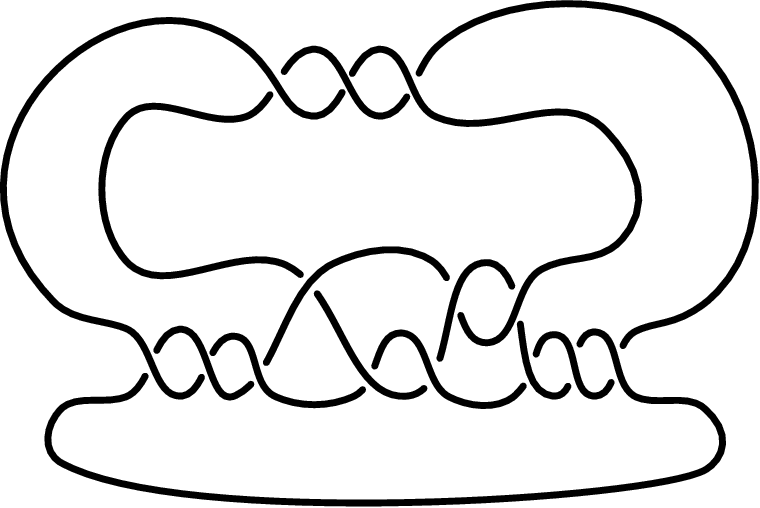
Case 1:
Revisiting the form of type (1) braids we have
where and for at least one value . Up to conjugation, this braid is equivalent to
where now , and for .
Notice that in this alternate expression the case can arise, in which case the braid in question takes the form where . Now recalling that we have
up to conjugation, where . The cases and give rise to the branch sets and , respectively, so the fundamental groups of the corresponding two-fold branched covers contain torsion and cannot be left-orderable. On the other hand, the closure of the braid gives a diagram with white graph satisfying the hypothesis of Proposition 8 (where the unbounded region is shaded black in the checkerboard colouring). We remark that, since this particular branch set is a pretzel knot, the two-fold branched cover is a Seifert fibred L-space. As a result, the desired conclusion may also be obtained from [2, Theorem 4].
Now assume that . Up to conjugation, we have the braid
where . Renaming constants, this braid may be expressed as
where for , for and . An example is given in Figure 3; the associated white graph (shading the unbounded region black) satisfies the hypothesis of Proposition 8.
Case 2:
As above, up to conjugation, consider the braids
where and for at least one value . Notice that if then and the braid in question is so that the relevant branch set is . Otherwise, and renaming constants as before we have the braid
where for and for . Notice in particular that . Now up to exchanging and taking mirrors (the former is cosmetic; the latter results in an orientation reversing homeomorphism in the two-fold branched cover) this braid is equivalent to
as in the case (this time with and ), so that the associated white graph satisfies the hypothesis of Proposition 8. ∎
References
- [1] John A. Baldwin. Heegaard Floer homology and genus one, one-boundary component open books. J. Topol., 1(4):963–992, 2008.
- [2] Steven Boyer, Cameron Gordon, and Liam Watson. On L-spaces and left-orderable fundamental groups. Preprint, arXiv:1107.5016.
- [3] Steven Boyer, Dale Rolfsen, and Bert Wiest. Orderable 3-manifold groups. Ann. Inst. Fourier (Grenoble), 55(1):243–288, 2005.
- [4] Adam Clay and Liam Watson. Left-orderable fundamental groups and Dehn surgery. Preprint, arXiv:1009.4176.
- [5] Adam Clay and Liam Watson. On cabled knots, Dehn surgery, and left-orderable fundamental groups. To appear in Math. Res. Lett., arXiv:1103.2358.
- [6] Joshua E. Greene. A spanning tree model for the Heegaard Floer homology of a branched double-cover. To appear in J. Topol., arXiv:0805.1381.
- [7] Joshua E. Greene. Alternating links and left-orderability. Preprint, arXiv:1107.5232.
- [8] Tetsuya Ito. Non-left-orderable double branched coverings. Preprint, arXiv:1106.1499.
- [9] Kunio Murasugi. On closed -braids. American Mathematical Society, Providence, R.I., 1974. Memoirs of the American Mathmatical Society, No. 151.
- [10] Peter Ozsváth and Zoltán Szabó. On knot Floer homology and lens space surgeries. Topology, 44(6):1281–1300, 2005.
- [11] Peter Ozsváth and Zoltán Szabó. On the Heegaard Floer homology of branched double-covers. Adv. Math., 194(1):1–33, 2005.
- [12] Thomas Peters. On L-spaces and non left-orderable 3-manifold groups. Preprint, arXiv:0903.4495.
- [13] Peter Scott. The geometries of -manifolds. Bull. London Math. Soc., 15(5):401–487, 1983.
- [14] Liam Watson. A surgical perspective on quasi-alternating links. To appear in Low-Dimensional and Symplectic Topology, volume 82 of Proc. Sympos. Pure Math., arXiv:0910.0449.