Testing General Relativity at Cosmological Scales: Implementation and Parameter Correlations
Abstract
The testing of general relativity at cosmological scales has become a possible and timely endeavor that is not only motivated by the pressing question of cosmic acceleration but also by the proposals of some extensions to general relativity that would manifest themselves at large scales of distance. We analyze here correlations between modified gravity growth parameters and some core cosmological parameters using the latest cosmological data sets including the refined Cosmic Evolution Survey 3D weak lensing. We provide the parametrized modified growth equations and their evolution. We implement known functional and binning approaches, and propose a new hybrid approach to evolve the modified gravity parameters in redshift (time) and scale. The hybrid parametrization combines a binned redshift dependence and a smooth evolution in scale avoiding a jump in the matter power spectrum. The formalism developed to test the consistency of current and future data with general relativity is implemented in a package that we make publicly available and call ISiTGR (Integrated Software in Testing General Relativity), an integrated set of modified modules for the publicly available packages CosmoMC and CAMB, including a modified version of the integrated Sachs-Wolfe-galaxy cross correlation module of Ho et al and a new weak-lensing likelihood module for the refined Hubble Space Telescope Cosmic Evolution Survey weak gravitational lensing tomography data. We obtain parameter constraints and correlation coefficients finding that modified gravity parameters are significantly correlated with and mildly correlated with , for all evolution methods. The degeneracies between and modified gravity parameters are found to be substantial for the functional form and also for some specific bins in the hybrid and binned methods indicating that these degeneracies will need to be taken into consideration when using future high precision data.
pacs
95.36.+x,98.80.Es,98.62.SbI introduction
There has been a growing interest in testing general relativity (GR) at cosmological scales. This has been triggered by the quest to understand the origin of cosmic acceleration which is one of the biggest puzzles in cosmology today. Specifically, one would like to test whether cosmic acceleration is due to some unknown, ”dark energy” component in the Universe or rather an extension or modification to gravity physics on cosmological scales. The growth rate of large scale structure proved to be a solid discriminator between these two possible explanations for cosmic acceleration and has been studied within this context by a number of papers. For example, some early papers explored inconsistencies between parameter constraints derived using observations that depended primarily on the growth rate of structure versus constraints derived from observations that probed only the expansion history. The presence of such inconsistencies would call into question the underlying gravity theory (see [1, 2, 4, 3]). These were followed by a number of papers using certain growth parameters that take distinct values for different gravity theories (see [5, 9, 10, 11, 19, 12, 22, 21, 28, 20, 13, 6, 29, 7, 8, 14, 16, 15, 17, 18, 23, 24, 25, 26, 27, 30, 31, 32, 33, 34, 35, 36, 37, 38, 39, 40, 41, 42, 43, 44, 45]). In this second approach, some parameters characterizing the growth rate are introduced in order to parametrize deviations from GR. These parameters have known values in GR but different values in modified gravity theories. So one possible goal is to constrain these parameters, in addition to the usual cosmological parameters, and see if they are consistent or not with the GR values. Also, recently Basilakos et al. proposed using the evolution of the linear bias as a way to test for deviations from GR [46].
These approaches have been applied using current available data sets and future simulated ones and in order to constrain growth parameters related to modifications of the perturbed Einstein equations in an effort to look for any indications of deviations from GR, but so far, none have been detected [47, 48, 49, 50, 51, 52, 53, 54, 55, 56, 57].
In this paper, we study correlations between modified gravity parameters and core cosmological parameters. We implement the evolution in time and scale of the modified gravity parameters using a functional form method and a binning method. We also propose and implement a new hybrid method that combines both. In the hybrid method, the evolution in time is represented in two redshift bins while the scale evolution follows a monotonic functional form. This provides a smooth evolution in scale combined with a binned redshift (time) dependence that was shown to be more robust than time functional forms as we discuss in the next section, see also [56, 53, 58]. We also describe the numerical framework that we introduce here as the package: Integrated Software in Testing General Relativity, ISiTGR (pronounced Is it GR and available publicly at http://www.utdallas.edu/~jdossett/isitgr/). ISiTGR is an integrated set of modified modules for the publicly available packages CosmoMC [59] and CAMB [60]. It combines all the modifications to those packages and a modified version to the of the Integrated Sachs-Wolfe (ISW)-galaxy cross correlations module by Ho et al. [61, 62] to test GR. We also include our weak-lensing likelihood module for the recently refined Hubble Space Telescope (HST) Cosmic Evolution Survey (COSMOS) weak-lensing tomography analysis in [63] which has also been modified to test GR, and a new baryon acoustic oscillation (BAO) likelihood module for the recently released WiggleZ Dark Energy Survey BAO measurement data [64].
II Parametrizing Deviations of the Growth Equations from General Relativity
II.1 Growth Equations in General Relativity
In the conformal Newtonian gauge the perturbed Friedmann-Lemaitre-Robertson-Walker (FLRW) metric is written as
| (1) |
where is the scale factor normalized to 1 today, the ’s are the comoving coordinates, and is conformal time. and are scalar potentials describing the scalar mode of the metric perturbations.
Using the first-order perturbed Einstein equations, while working in Fourier space, we can get two very useful equations that describe the evolution of the scalar potentials. The combination of the time-time and time-space equations gives the Poisson equation describing the potential . Then, to relate the two potentials to one another we take the traceless, space-space component of these equations. Explicitly, these equations are
| (2) | |||||
| (3) |
where and are the density and the shear stress, respectively, for matter species, . is the gauge-invariant, rest-frame overdensity for matter species, , the evolution of which describes the growth of inhomogeneities. It is defined by
| (4) |
where is the Hubble factor in conformal time, and for species , is the fractional overdensity and is the heat flux and is related to the divergence of the peculiar velocity, , by . Enforcing the conservation of energy momentum on the perturbed matter fluid, these quantities for uncoupled fluid species or the mass-averaged quantities for all the fluids evolve as described in [65]:
| (5) | |||||
| (6) |
Above, is the equation of state. Combining these two equations, we can express the evolution of by
| (7) |
II.2 Modified Gravity Growth Parameters
Parametrizing both modifications to Poisson’s equation, (2), as well as the ratio between the two metric potentials and in the perturbed FLRW metric (called gravitational slip by Caldwell et al. [11]) has recently been the subject of a lot of the work on testing general relativity; see, for example, [11, 49, 53, 50, 51, 52]. The parameters we use in this paper to describe modifications to the growth [modified gravity MG parameters] are based upon those used in [50].
The parametrized modifications to the growth equations proposed by [50] directly modify Eqs. (2) and (3) and make no assumptions as to the time when a deviation from GR is allowed. These modifications are as follows:
| (8) | |||||
| (9) |
where and are the MG parameters. The parameter represents a modification to the Poisson equation, while the parameter quantifies the gravitational slip (at late times, when anisotropic stress is negligible, ). In our code, rather than using the parameter which is degenerate with , we instead use the parameter as suggested in [50] (this parameter is equivalent to the parameter in [45, 53] or of [52]). Combining Eqs. (8) and (9), we arrive at the second modified growth equation used in this paper:
| (10) |
So, the modified growth equations are (8) and (10), and and are now the MG parameters. As discussed in our previous work [56], this approach of using the parameter instead of is also useful because observations of the weak-lensing and ISW are sensitive to the sum of the metric potentials and its time derivative respectively. Thus observations are able to give us direct measurements of this parameter.
II.3 Different Approaches to Evolving Modified Growth Parameters in Time and Scale
To date, there have primarily been two approaches to evolving the MG parameters in time and scale; one using a continuous functional form and the other based on binning. We implement in ISiTGR the two approaches and, additionally, a new hybrid approach, as we explain below.
The first approach involves defining a functional form for each parameter that allows it to evolve monotonically in both time and scale. This allows one to make no assumptions as to when a deviation from general relativity is allowed. Such an approach was taken in for example [50]. In that work the functional form,
| (11) |
was assumed, where denotes either or in Eqs. (8) and (9). Thus a total of six model parameters are used to test GR: , , , , , and . The parameters and parametrize time and scale dependence respectively, with GR values and . and are the present-day superhorizon values while and are the present-day subhorizon values of the and , all taking GR values of .
In the second approach, instead of evolving each of the parameters assuming some functional form, one can bin the MG parameters. This approach allows the parameters to take on different values in predefined redshift and scale bins. This technique was used in, for example, [53, 52]. In those works two redshift and two scale bins were defined and for redshifts above a certain critical redshift, GR was assumed to be valid. In each bin the parameters were allowed to take on different values resulting in a total of eight model parameters used to test GR.
The third approach that we propose here is a hybrid one where the evolution in redshift (or time) is binned into two redshift bins, but the evolution in scale evolves monotonically in the same way as the functional form above. Our motivation for this hybrid binning approach is that it takes advantage of an evolution in scale that is not so abrupt as that in the traditional binning method, while still taking advantage of a redshift (time) dependence expressed in the form of bins, which was shown to be more robust than time functional forms [56, 53, 58]. For example, in [56], we found that binning methods do not display the extent of tensions between the MG parameters (preferred by different data sets) as in the functional form method, where tensions are exacerbated by the chosen functional form. Also, in Ref. [58], the author found similar to what we noticed and that the constraints on MG parameters depend strongly on the parameter (the scale factor exponent in the functional parametrization). They further looked at ways to remove this strong dependence on the parameter suggesting and exploring binning as a solution.
To take advantage of all these techniques, we have developed two versions of our code. One version of the code uses the functional form (11). It provides the option to apply the functional form (11) to either and (as done in [50]) or and . The other version of the code is based on binning methods. It provides the option of the second approach with traditional binning (described above), or alternatively the third, hybrid approach with two redshift bins, but the evolution in scale evolves monotonically.
 |
In the binning version of the code, we evolve only and . Transitions between the redshift bin are evolved following [44, 53] and use a hyperbolic tangent function with a transition width . In this way the binning can actually be written functionally as (with representing or )
| (12) |
where is the redshift where the transition between the two redshift bins occurs and is the redshift below which GR is to be tested. We hard code to give us equally sized bins, but this of course is optional and can easily be changed. represents the binning method for in the th bin. For the suggested hybrid method it has the form
| (13) | |||||
while with traditional binning in principle evolves as
Here though, we have rather chosen to implement the traditional binning method with some control on the transition as:
| (20) | |||||
where is the transition width between bins. We set since we want to imitate traditional binning and ensure the transition between the bins is very rapid compared to the scale at which the transition occurs, thus the evolution maintains the appearance of being described by actual bins while having a functional definition. Although can be used to smooth the transition between the bins but doing so to remove the appearance of actual bins also hinders the users ability to control the value of the MG parameters at , as is easily done in the hybrid method. We leave it to the users to choose their favorite method.
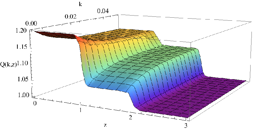
To further illustrate the hybrid evolution, in Fig. 1 we plot an example of the evolution of the MG parameter using this new hybrid form with . In this figure, one can see the binned aspect of the MG parameter evolution in redshift space, while the evolution in scale, -space, evolves monotonically. The advantages to this smooth evolution in scale are illustrated further in Fig. 2, where we compare the matter power spectrum produced using an identical set of parameters. The hybrid method produces a much more physical and smooth matter power spectrum.
 |
III Modified Gravity Growth Equations and Numerical Implementations
III.1 Synchronous Gauge Variables and CMB Implementation
We will first focus on our modifications to the publicly available code CAMB (Code for Anisotropies in the Microwave Background) [60] which calculates the various CMB anisotropy spectra (, , , ) as well as the three-dimensional matter power spectrum . These observables are very powerful in constraining both the growth history of structure in the Universe as well as the expansion history of the Universe, and thus are very useful in constraining the parameters we use to test general relativity.
CAMB is written in the synchronous gauge. Instead of using the metric potentials and of the conformal Newtonian gauge, it uses the metric potentials and consistent with the notation of Ma and Bertschinger [65]. From Eq. (18) of [65], we know the metric potentials in the two gauges are related to one another by
| (21) | |||||
| (22) | |||||
| (23) |
CAMB evolves the metric potential (actually evolving ) as well as the matter perturbations, , heat flux,, and the shear stress for each matter species in the synchronous gauge according to the evolution equations given in [65]. Additionally, the CAMB variables and are evaluated at each time step. They are useful for defining the evolution of the matter perturbations and are defined as
| (24) | |||
| (25) |
Using these variables allows CAMB to be written in such a way that the evolution of all other variables is changed simply by adjusting the evolution of the metric potential . Thus it is important that we derive an equation for the evolution of consistent with the modified growth equations (8) and (10). To do this, we begin by subbing (21) into (8) and taking the time derivative. This gives
| (26) |
where . Next subbing (8) and (22) into (10) gives an expression for :
| (27) |
Now subbing Eqs. (7), (27), as well as the time derivative of from matter conservation into (26) we get
| (28) |
where
| (29) |
Next we can sub in for and in Eq. (28) by using (22) and the time derivative of (21). This gives:
| (30) |
We want an equation where all the variables on the right-hand-side are in the synchronous gauge, as those are the variables evolved by CAMB. We already know that and are gauge invariant, so we need not worry about them. However the in the above equations is still in the conformal Newtonian gauge. It transforms to the synchronous gauge according to Eq. 27b of [65] which by converting, as described above, from to can be written as
| (31) |
So finally subbing (31) into (30) and collecting the terms we have [equivalent to Eq. A8 in [50]]
| (32) |
with
| (33) |
After the metric potentials and matter perturbations are evolved the next major change is to redefine the derivatives of the Newtonian metric potentials, , which go into evaluating the ISW effect in the CMB temperature anisotropy. We can get this quantity quickly by applying our knowledge that the quantities and are invariant in transformations between the synchronous and conformal Newtonian gauges. Thus simply taking the time derivative of (10) and subbing in for and we get:
| (34) | |||
Other small changes to the scalar source term are necessary and were calculated using a slightly modified version of the Maple worksheet lineofsight.txt available from [60].
Some additional modifications though still remain to alleviate problems caused by the likely possibility that bad combinations of MG parameters will be introduced to CAMB by the sampling routine of CosmoMC. We encountered three routines which routinely ran into problems with bad combinations of MG parameters, the reionization module, the halofit module and the CMB lensing module. To alleviate these issues we added error variables to these routines where in the event a bad parameter combination causes these modules to fail, the calculation is aborted and that parameter combination is rejected rather than causing the CosmoMC to stop. With all of these changes in place CAMB is able to calculate and output all the modified CMB spectra as well as the modified matter power spectrum.
III.2 Weak-Lensing Implementation
Weak-lensing tomography shear-shear cross correlations are useful to constrain both the expansion history and the growth history of structure in the Universe. As discussed above this data can give us direct measurements of the parameter ,;thus it is important to have a module for CosmoMC which takes advantage of this data. Here we discuss our module using the weak-lensing tomography shear-shear cross correlations of the HST-COSMOS survey recently compiled by Schrabback et. al. [63]. It is worth noting here that this data set probes scales on which perturbations are not described by linear theory alone. The parametrized modified growth equations (8) and (10) describe deviations from GR on linear scales only. Though we use the halofit module to describe the nonlinear part of the power-spectrum, it should be noted that this may not be completely accurate and should be considered a source of possible systematic error for our MG parameter constraints. The authors of [63] perform a refined analysis of the HST-COSMOS survey of [66], in combination with the COSMOS-30 photometric redshift catalog provided by [67]. The shear-shear cross correlations were calculated between 6 redshift bins, , , , , and a sixth bin that contains all faint galaxies with a numerically estimated redshift distribution from ; see Fig. 6 of [63]. Certain exclusions were made as described in [63], such as the luminous red galaxies (LRGs) to avoid G-I intrinsic alignment bias and the lowest angular theta bin because of model uncertainties. Only bright galaxies () were used in the first bin . Also, autocorrelations were not used in bins to reduce the effect of I-I intrinsic alignments. We modified the publicly available code for the COSMOS 3D weak-lensing built by Lesgourgues et. al. [68] to incorporate the shear cross correlations as seen in, for example, [63] and the MG parameters.
The shear cross correlation functions between bins are given by
| (35) |
where is the -order Bessel function of the first kind, is the modulus of the two-dimensional wave vector, and is the convergence cross-power spectra between bins .
In order to evaluate the convergence cross-power spectra, let us first recall that working with the metric (1), the convergence is defined as
| (36) |
with comoving radial distance , comoving distance to the horizon ,comoving angular diameter distance , and the weighted geometric lens-efficiency factor given by
| (37) |
corresponding to the galaxy redshift distributions . Applying the Limber approximation to (36) to get the convergence cross power spectrum in the absence of any modifications of growth gives us the usual result in terms of the three-dimensional (nonlinear) power spectrum :
| (38) |
where is the weighted geometric lens-efficiency factor as defined above corresponding to the redshift bin.
Now to incorporate our MG parametrization we substitute the late-time form (ie. negligible anisotropic stress) of (10) into (36) and again apply the Limber approximation. This gives us a modified convergence cross power spectrum that takes into account our MG parametrization:
| (39) |
In calculating our cross correlation functions we follow instructions from [63] and weight the predictions for the bin, , with logarithmic spaced upper and lower limits and , respectively, based on the number of galaxy pairs, for a given as
| (40) |
To evaluate the likelihood we use the dimensional covariance matrix for the corresponding weak shear correlations provided by Schrabback et. al. [63] applying the correction to the inverse covariance, , seen in [63, 70], as
| (41) |
for independent realizations and a dimensional data vector. We then account for the uncertainty in the numerical estimate of the galaxy redshift distribution of bin six, , by marginalizing over the nuisance parameter which is applied following [63] where for the sixth bin we instead use the galaxy redshift distribution given by . Now the likelihood () is given by:
| (42) |
III.3 ISW-Galaxy Cross Correlations Implementation
As discussed in, for example, [50, 53, 52], cross correlations between the ISW effect and the galaxy density can be very useful in constraining the MG parameters. Thus, we modified the publicly available module by Ho et al.[61, 62] for calculating these cross correlations in the presence of a modification to gravity described by Eqs. (8) and (10). Let us review some of the details of calculating these cross correlations.
First recall, when working with the perturbed FLRW metric (1) that the CMB temperature anisotropy due to the ISW effect can be written as [61]
| (43) |
where is the conformal time of recombination and is the conformal time today. The angular galaxy density fluctuations that we want to cross correlate these temperature fluctuations with are
| (44) |
where is the galaxy bias, is the normalized selection function, and is the comoving angular diameter distance redshift .
Following [61], we can once again use the Limber approximation to write the cross-power spectrum between these two fields in the absence of any modifications to the growth as
| (45) |
where the growth factor [please note that this is not the parameter we use to test GR] is calculated using the standard differential equation for at linear scales, with given in Eq. (46). This result was attained by considering at late times in GR the potentials in (43) can be written combining to (2) and (3) as
| (46) |
When testing general relativity though, Eq. (46) no longer holds and we must instead, as with the weak-lensing cross correlations, refer to the late-time version of (10) giving
| (47) |
With these changes the ISW-galaxy cross power spectrum is given by:
| (48) |
Additionally, to fully account for the gravity modifications, the differential equation used to calculate the in must be modified. Combining Eqs. (8) and (10) to get , the late-time form of differential equation for now reads
| (49) |
In order to correctly perform these cross correlations, the code by Ho et al. also corrects factor to account for a magnification bias on SDSS quasars and NVSS radio sources [61]. In calculating this magnification bias, the weak-lensing convergence must be considered on scales smaller than the Hubble distance [71]. Thus, we modify the code to account for changes in the weak-lensing convergence according to (36) and (10) but consider only large- values of the MG parameters for these corrections in calculating the magnification bias.
The original code by Ho et al. also has a likelihood code which uses cross correlations between weak-lensing of the CMB and the galaxy density. A detailed description of this part of the code is contained in [62]. We modify this portion of the code to account for the changes to the convergence in the presence of modifications to the growth as described by Eqs. (10) and (36).
III.4 WiggleZ Baryon Acoustic Oscillation Likelihood
Recently, the WiggleZ Dark Energy Survey released its full data set of BAO measurements [64]. We include a likelihood module for this data set in ISiTGR. Let us quickly review the likelihood calculation for this data.
The data set released by [64] includes measurements of the acoustic parameter at three different effective redshifts: , , and . The acoustic parameter was first introduced by [72] and is defined as
| (50) |
where is the physical matter density. is the effective distance defined by:
| (51) |
with the angular diameter distance to the redshift , .
To calculate the likelihood, the theoretical value of is calculated at each of the effective redshifts. Then using the covariance matrix for the data given in [64], the likelihood for a given model is expressed as
| (52) |
 |
 |
 |
 |
 |
| Correlation coefficients between and and the MG parameters | ||||||||
| MG parameters evolved using traditional binning | ||||||||
| Parameter | ||||||||
| 0.0116 | -0.0535 | -0.0338 | -0.0371 | 0.0114 | -0.0988 | 0.0190 | -0.0818 | |
| 0.0937 | 0.1540 | -0.1583 | -0.4267 | 0.2093 | 0.2857 | 0.2377 | 0.0185 | |
| MG parameters evolved using hybrid binning | ||||||||
| Parameter | ||||||||
| 0.1571 | -0.1639 | -0.003 | -0.0105 | 0.1814 | -0.2172 | -0.0056 | -0.0070 | |
| 0.1692 | 0.4282 | -0.1076 | 0.1676 | 0.2147 | 0.5390 | 0.1937 | 0.0716 | |
| MG parameters evolved using the functional form | |||
|---|---|---|---|
| Parameter | |||
| -0.1173 | -0.0294 | 0.0542 | |
| -0.5409 | -0.2631 | 0.5742 | |
 |
 |
 |
 |
 |
IV Correlations obtained between cosmological parameters and modified gravity growth parameters
We provide here our results about various constraints and correlation coefficients found between core cosmological parameters and modified growth parameters. We use the standard definition for the correlation coefficient:
| (53) |
where , are the parameters, is the covariance of the two parameters, and and are their respective standard deviations.
In addition to varying a given set of modified gravity parameters, we vary the six core cosmological parameters: and the , the baryon and cold-dark matter physical density parameters, respectively; , the ratio of the sound horizon to the angular diameter distance of the surface of last scattering; , the reionization optical depth; , the spectral index; and , the amplitude of the primordial power spectrum. Additionally, the results illustrated here always use the following data sets for expansion history constraints, WiggleZ BAO measurements [64], the supernovae Union2 compilation of the Supernovae Cosmology Project (SCP) [73] and references of other compiled supernovae (SN) therein. We also use the prior on km/s/Mpc given by [74], and a prior on the age of the Universe (AGE) GyrsAGEGyrs.
We include in our analysis the three parametrization approaches: functional form, binned method, and hybrid method.
First, we utilize the functional form to evolve the MG parameters. For simplicity, we choose to assume the modifications are scale-independent () and evolve the parameters and with the functional forms described by (11):
| (54) | |||||
| (55) |
So, in addition to varying the six core cosmological parameters listed above, we vary the MG parameters , (inferring from and ), and . To constrain these parameters we use all of the available data sets: the WMAP7 temperature and polarization spectra (CMB) [75], the matter power spectrum (MPK) from the Sloan Digital Sky Survey (SDSS) DR7 [76], the ISW-galaxy cross correlations [61, 62], and the refined HST-COSMOS weak-lensing tomography [63].
Second, we bin the MG parameters rather than evolve with some functional form. We bin traditionally in both and as described by (12) and (20) with , , , and :
| (56) | |||||
with
| (57) | |||||
| (58) | |||||
So, the -bins are and and GR is assumed for , while the -bins are and . We vary all eight MG parameters, , in addition to the six core cosmological parameters and again we use all of the available data sets: CMB, MPK, ISW, and WL.
Finally, we evolve the MG parameters using the newly introduced hybrid method with evolution with redshift () dependence identical to that of traditional binning method, Eq. (56), and scale () dependence described by Eq. (13) with :
| (59) | |||||
| (60) | |||||
So, just as with traditional binning, the -bins are and and GR is assumed for while the scale dependence transitions exponentially between two values for each redshift bin with a decay constant . We again vary all eight MG parameters, , in addition to the six core cosmological parameters and use all of the available data sets: CMB, MPK, ISW, and WL.
We plot the and 2D contours for the MG parameters in Figs. 3 and 4 for the three methods respectively. We find that the constraints on modified gravity parameters are consistent with general relativity for all methods; however, the correlations between these parameters and some cosmological parameters are significant as we describe below.
In Table 1, we report the results obtained for the correlation coefficients between the modified gravity parameters and cosmological parameters. The table shows that modified gravity parameters are significantly correlated with and mildly correlated with . For example, the degeneracies between and modified gravity parameters are found to be substantial, especially for the functional form evolution method where , , and . For the hybrid method, about half of the bins seem to present some strong correlations, with the strongest being . The traditional binning method seems to present less correlation than the hybrid method, but again about half of the bins have strong correlations with the largest being .
Correlations between MG parameters and have been discussed briefly by [52]. They too found that the correlations were significant. We find that for both the hybrid and traditional binning method that correlations between and the parameters are positive meaning higher values of gives rise to higher values of . We also find that, with the exception of the parameter , the high parameters are more strongly correlated than the low parameters, agreeing with the conclusions of [52] that these correlations are strongly dependent on the matter power spectrum, weak lensing, and ISW data sets. The corresponding plots are given in Figs. 5, 6, and 7, for the functional form method, traditional binning method, and hybrid method respectively. Looking at Fig. 6 we can see that there is not much difference between the slope of contours for and or , while the correlations coefficients given in Table 1 are much larger for this can be explained by the bulges in each of those contours. For this bulge is toward the higher values of that parameter and at higher values of thereby increasing the positive correlation, while for this bulge prefers lower values of said parameter, but still higher values of presenting an anticorrelation that washes out the underling positive correlation of the rest of the parameter space. These bulges are caused by parameter constraints that are not completely Gaussian, as also seen in Fig. 4. Non-Gaussianity in the constraints also accounts for the odd shapes of the contours in Fig. 5, showing the correlations for the functional form MG parameters.
V Conclusion
Testing general relativity on cosmological scales is a topic of great interest in cosmology today. It allows an exploration of the origin of cosmic acceleration, as well as testing possible extensions to general relativity. Future high precision data will allow us to test gravity on cosmological scales to a very high level of precision. In this work we focused on the presence of correlations between modified gravity growth parameters and core cosmological parameters finding that some of them can be very strong. We provided the underlying modified growth equations and their evolution. We implemented the time and scale dependencies of the MG parameters using a functional form method, a binning method, as well as, a new hybrid method. The hybrid method provides a smooth evolution in scale and a binned redshift (time) dependence that was shown to be more robust than time functional forms. We used the most recent available cosmological data sets including BAO measurements from the WiggleZ Dark Energy Survey [64] as well as the Two-Degree Field and DR7 Sloan Digital Sky surveys [76, 77]; priors on from [74]; the Wilkinson Microwave Anisotropy Probe (WMAP) 7-year CMB temperature and polarization spectra [75]; the supernovae Union2 compilation, which includes the 557 type-Ia SCP [73] and references of other compiled supernovae therein; the MPK from the SDSS DR7 [76]; the ISW-galaxy cross correlations using the 2MASS and SDSS LRG galaxy surveys [61, 62]; and the recently refined HST-COSMOS weak-lensing tomography analysis in [63]. We also described our implementation of the modified growth equations into a numerical framework, ISiTGR, an integrated set of modified modules for the packages CosmoMC [59] and CAMB [60] to be used to this end. ISiTGR modifies multiple publicly available codes: CAMB [60], CosmoMC [59], the ISW-galaxy cross correlation code [61, 62], and the original COSMOS weak-lensing code [68]. When using and referring to this package, the original codes should also be cited, as well as the above data sets when used in a particular analysis. Our analysis found that strong correlations between and modified gravity parameters are present, in addition to mild correlations with other cosmological parameters such as . The degeneracies between and modified gravity parameters are substantial for the functional form and also for nearly half of the bins in the hybrid and binned methods. These degeneracies will need to be addressed when using future high precision data to perform these tests.
Acknowledgements.
We thank T. Schrabback for providing the refined HST COSMOS data. We thank A. Lewis for useful comments. M.I. acknowledges that this material is based upon work supported by the Department of Energy (DOE) under Grant No. DE-FG02-10ER41310, NASA under Grant No. NNX09AJ55G, and that part of the calculations for this work have been performed on the Cosmology Computer Cluster funded by the Hoblitzelle Foundation. J.D. acknowledges that this research was supported in part by the DOE Office of Science Graduate Fellowship Program (SCGF). The DOE SCGF Program was made possible in part by the American Recovery and Reinvestment Act of 2009. The DOE SCGF program is administered by the Oak Ridge Institute for Science and Education for the DOE. ORISE is managed by Oak Ridge Associated Universities (ORAU) under DOE Contract No. DE-AC05-06OR23100.References
- [1] A. Lue, R. Scoccimarro, and G. Starkman, Phys. Rev. D.69, 124015 (2004).
- [2] Y. S. Song, Phys. Rev. D.71, 024026 (2005).
- [3] L. Knox, Y.S. Song, and J. A. Tyson, Phys. Rev. D.74, 023512 (2006), arXiv:astro-ph/0503644.
- [4] M. Ishak, A. Upadhye, and D. Spergel, Phys. Rev. D.74, 043513 (2006), arXiv:astro-ph/0507184.
- [5] E. Linder, Phys. Rev. D.72, 043529 (2005), arXiv:astro-ph/0507263.
- [6] T. Koivisto and D. F. Mota, Phys. Rev. D.73, 083502,(2006).
- [7] K. Koyama, J. Cosmol. Astropart. Phys.03 (2006) 017, arXiv:astro-ph/0601220.
- [8] P. Zhang, Phys. Rev. D.73, 123504 (2006), arXiv:astro-ph/0511218.
- [9] P.J. Zhang, M. Liguori, R. Bean, and S. Dodelson, Phys.Rev.Lett. 99, 141302 (2007), arXiv:0704.1932.
- [10] W. Hu and I. Sawicki, Phys. Rev. D 76, 104043 (2007).
- [11] R. Caldwell, A. Cooray, and A. Melchiorri, Phys. Rev. D.76, 023507 (2007), arXiv:astro-ph/0703375.
- [12] M. Kunz and D. Sapone, Phys. Rev. Lett. 98, 121301 (2007), arXiv:astro-ph/0612452.
- [13] D. Huterer and E. Linder, Phys. Rev. D.75, 023519 (2007), arXiv:astro-ph/0608681.
- [14] E. Linder and R. Cahn, Astropart. Phys. 28, 481 (2007), arXiv:astro-ph/0701317.
- [15] O. Dore et. al, (2007) arXiv: 0712.1599.
- [16] Y. S. Song, I. Sawicki, W. Hu, Phys. Rev. D.75, 064003 (2007), arXiv:astro-ph/0606286.
- [17] G. Gabadadze and A. Igelsias, Classical Quantum Gravity 25, 154008 (2008), arXiv:0712.4086.
- [18] D. Polarski and R. Gannouji, Phys. Lett. B. 660, 439 (2008), arXiv:0710.1510.
- [19] V. Acquaviva, A. Hajian, D. Spergel, and S. Das, Phys. Rev. D.78, 043514 (2008), arXiv:0803.2236.
- [20] E. Bertschinger and P. Zukin, Phys. Rev. D.78, 024015 (2008), arXiv:0801.2431.
- [21] S. Daniel, R. Caldwell, A. Cooray, and A. Melchiorri Phys. Rev. D.77, 103513 (2008), arXiv:0802.1068.
- [22] Y. Gong, Phys. Rev. D.78, 123010 (2008), arXiv:0808.1316.
- [23] W. Hu, Phys. Rev. D.77, 103524 (2008), arXiv:0801.2433.
- [24] B. Jain and P. Zhang, Phys. Rev. D.78, 063503 (2008), arXiv:0709.2375.
- [25] H. Wei and N. Zhang, Phys. Rev. D.78, 023011 (2008), arXiv: 0803.3292.
- [26] J. Dent, S. Dutta, and L. Perivolaropoulos, Phys. Rev. D.80, 023514 (2009), arXiv:0903.5296.
- [27] X. Fu, P. Wu, H. Yu, Phys. Lett. B 677, 12 (2009), arXiv:0905.1735.
- [28] Y. Gong, M. Ishak, and A. Wang, Phys. Rev. D.80, 023002 (2009), arXiv:0903.0001.
- [29] R. Gannouji, B. Moraes and D. Polarski, arXiv:0907.0393.
- [30] M. Ishak and J. Dossett, Phys. Rev. D.80, 043004 (2009), arXiv:0905.2470.
- [31] E. Linder, Phys. Rev. D.79, 063519 (2009), arXiv:0901.0918.
- [32] P. Serra, A. Cooray, S. Daniel, R. Caldwell, and A. Melchiorri, Phys. Rev. D 79, 101301 (2009), arXiv:0901.0917.
- [33] Y. S. Song and O. Dore, J. Cosmol. Astropart. Phys.03 (2009) 025, arXiv:0812.0002.
- [34] Y.S. Song and W. Percival, J. Cosmol. Astropart. Phys.10 (2009) 004, arXiv:0807.0810.
- [35] S. Thomas, F. Abdalla and J. Weller, Mon. Not. R. Astron. Soc.395, 197 (2009), arXiv:0810.2269.
- [36] S. Tsujikawa, R. Gannouji, B. Moraes and D. Polarski, Phys. Rev. D.80, 084044 (2009), arXiv:0908.2269.
- [37] P. Wu, H. Yu and X. Fu, J. Cosmol. Astropart. Phys.06 (2009) 019, arXiv:0905:3444.
- [38] G. Zhao, L. Pogosian, A. Silvestri and J. Zylberberg, Phys. Rev. D.79, 083513 (2009), arXiv:0809.3791.
- [39] G. Zhao, L. Pogosian, A. Silvestri, and J. Zylberberg, Phys. Rev. Lett. 103, 241301 (2009), arXiv:0905.1326.
- [40] V. Acquaviva and E. Gawiser, Phys. Rev. D.82, 082001 (2010), arXiv:1008.3392.
- [41] J. Dossett, M. Ishak, J. Moldenhauer, Y. Gong, A. Wang, J. Cosmol. Astropart. Phys.04 (2010) 022, arXiv:1004.3086.
- [42] P. Ferreira and C. Skordis, Phys. Rev. D.81, 104020 (2010), arXiv:1003.4231.
- [43] J. Jing and S. Chen, Phys. Lett. B 685, 185 (2010), arXiv:0908.4379.
- [44] L. Pogosian, A. Sivestri,K. Koyama, and G. Zhao, Phys. Rev. D.81, 104023 (2010), arXiv:1002.2382.
- [45] Y. S. Song, L. Hollenstein, G. Caldera-Cabral, and K. Koyama, J. Cosmol. Astropart. Phys.04 (2010) 018, arXiv:1001.0969.
- [46] S. Basilakos, M. Plionis, and A. Pouri, Phys. Rev. D.83, 123525 (2011), arXiv:1106.1183.
- [47] S. Wang, L. Hui, M. May, and Z. Haiman, Phys. Rev. D.76, 063503 (2007), arXiv:0705.0165.
- [48] M. Ishak, Foundation of Physics Journal 37, 1470 (2007), astro-ph/0504416.
- [49] S. Daniel, R. Caldwell, A. Cooray, P. Serra, and A. Melchiorri, Phys. Rev. D.80, 023532 (2009), arXiv:0901.0919.
- [50] R. Bean and M. Tangmatitham, Phys. Rev. D.81, 083534 (2010), arXiv:1002.4197.
- [51] S. Daniel, E. Linder, T. Smith, R. Caldwell, A. Corray, A Leauthaud, and L. Lombriser, Phys. Rev. D 81, 123508 (2010), arXiv:1002.1962.
- [52] S. Daniel and E. Linder Phys. Rev. D.82, 103523 (2010), arXiv:1008.0397.
- [53] G. Zhao et. al. Phys. Rev. D.81, 103510 (2010), arXiv:1003.0001.
- [54] L. Lombriser, Phys. Rev. D.83, 063519 (2011), arXiv:1101.0594.
- [55] I. Toreno, E. Semboloni, and T. Schrabback, Astron. Astrophys. 530, A68 (2011), arXiv:1012.5854.
- [56] J. Dossett, J. Moldenhauer, and M. Ishak, Phys. Rev. D.84, 023012, (2011), arXiv:1103.1195.
- [57] A. Hojjati, L. Pogosian, G. Zhao, J. Cosmol. Astropart. Phys.08 (2011) 005, arXiv:1106.4543.
- [58] Y. S. Song, G. B. Zhao, D. Bacon, K. Koyama, R. C. Nichol, and L. Pogosian, Phys. Rev. D.84, 083523 (2011), arXiv:1011.2106.
- [59] A. Lewis and S. Bridle, Phys. Rev. D.66, 103511 (2002). http://cosmologist.info/cosmomc/.
- [60] A. Lewis, A. Challinor, and A. Lasenby, Astrophys. J. 538, 473 (2000); http://camb.info.
- [61] S. Ho, C. Hirata, N. Padmanabhan, U. Seljak, and N. Bahcall, Phys. Rev. D.78, 043519 (2008), arXiv:0801.0642.
- [62] C. Hirata, S. Ho, N.Padmanabhan, U. Seljak, and N. Bahcall, Phys. Rev. D.78, 043520 (2008), arXiv:0801.0644.
- [63] T. Schrabback et al., Astron. Astrophys. 516, A63 (2010), arXiv:0911.0053.
- [64] C. Blake et al. Accepted for publication in Mon. Not. R. Astron. Soc.(2011), arXiv:1108.2635.
- [65] C. Ma and E. Bertschinger, Astrophys. J. 455, 7 (1995).
- [66] N. Scoville, R. G. Abraham and H. Aussel, et. al., (2007), Astropys. J. Suppl. Ser. 172, 38 (2007).
- [67] O. Ilbert, P. Capak, and M. Salvato, et. al., Astrophys. J. 690, 1236 (2009).
- [68] J. Lesgourgues, M. Viel, M.G. Haehnelt, and R. Massey, J. Cosmol. Astropart. Phys.11 (2007) 008.
- [69] T. Schrabback, private communication.
- [70] J. Hartlap, P. Simon, and P. Schneider, Astron. Astrophys. 464, 399 (2007).
- [71] T. Matsubara, Astrophys. J. Lett. 537, L77 (2000), arXiv:astro-ph/0004392.
- [72] D. J. Eisenstein et al., Astrophys. J. 633, 560 (2005).
- [73] R. Amanullah et al., Astrophys. J. 716, 712 (2010), arXiv:1004.1711.
- [74] A.G. Riess et al., Astrophys. J. 659, 98 (2007).
- [75] J.Dunkley, E.Komatsu, D.L.Larson, and M.R.Nolta The WMAP Team likelihood http://lambda.gsfc.nasa.gov/; D. Larson et al., Astrophys. J. Suppl. Ser. 192, 16 (2011), arXiv:1001.4635; N. Jarosik et al., Astrophys. J. Suppl. Ser. 192, 14 (2011), arXiv:1001.4744; E. Komatsu et al., Astrophys. J. Suppl. Ser. 192, 18 (2011), arXiv:1001.4538.
- [76] B. A. Reid et al. Mon. Not. R. Astron. Soc.Volume 404, 60 (2010), arXiv:0907.1659.
- [77] W. J. Percival et al. Mon. Not. R. Astron. Soc.Volume 401, 2148 (2010), arXiv:0907.1660.