跳到论文正文
W Papers独立论文阅读器 arXiv:1109.4582 论文正文 计算阅读时间 · 0%
引用这篇论文根据当前论文元数据生成,正式投稿前建议核对。


License: arXiv.org perpetual non-exclusive license
arXiv:1109.4582v4 [math.AP] 22 Apr 2012

Statistics of wave functions for a point scatterer on the torus

Zeév Rudnick and Henrik Ueberschär Address: Raymond and Beverly Sackler School of Mathematical Sciences, Tel Aviv University, Tel Aviv 69978, Israel Email address: rudnick@post.tau.ac.il Address: Raymond and Beverly Sackler School of Mathematical Sciences, Tel Aviv University, Tel Aviv 69978, Israel Email address: henrik@post.tau.ac.il
Date: August 24, 2026
Abstract.

Quantum systems whose classical counterpart have ergodic dynamics are quantum ergodic in the sense that almost all eigenstates are uniformly distributed in phase space. In contrast, when the classical dynamics is integrable, there is concentration of eigenfunctions on invariant structures in phase space. In this paper we study eigenfunction statistics for the Laplacian perturbed by a delta-potential (also known as a point scatterer) on a flat torus, a popular model used to study the transition between integrability and chaos in quantum mechanics. The eigenfunctions of this operator consist of eigenfunctions of the Laplacian which vanish at the scatterer, and new, or perturbed, eigenfunctions. We show that almost all of the perturbed eigenfunctions are uniformly distributed in configuration space.

1. Introduction

Quantum systems whose classical counterpart have ergodic dynamics satisfy Schnirelman’s theorem, which asserts that almost all eigenstates are uniformly distributed in phase space in an appropriate sense [21, 7, 23]. In contrast, when the classical dynamics is integrable, there is concentration of eigenfunctions on invariant structures in phase space. In this paper we study eigenfunction statistics for an intermediate system, that of a point scatterer on the flat torus.

The use of point scatterers, or δ\delta-potentials, goes back to the Kronig-Penney model [13] which is an idealized solvable model used to explain conductivity in a solid crystal and the appearance of electronic band structure. They have also been studied in the mathematical literature to explain the spurious occurrence of the Riemann zeros in a numerical experiment [8]. Billiards with a point scatterer have been used extensively in the quantum chaos literature, starting with Seba [19], to model quantum systems strongly perturbed in a region smaller than the wavelength of the particle.

The flat torus is a standard example of a system for which the geodesic flow is completely integrable. Placing a scatterer at a point x0x_{0} in the torus does not change the classical dynamics except for a measure zero set of trajectories, and gives a quantum system whose dynamics is generated by an operator formally written as

(1.1) −Δ+α​δx0-\Delta+\alpha\delta_{x_{0}}

with δx0\delta_{x_{0}} being the Dirac mass at x0x_{0} and α\alpha being a coupling parameter. Mathematically this corresponds to picking a self-adjoint extension of the Laplacian −Δ-\Delta acting on functions vanishing near x0x_{0} (see Section § 3 and Appendix § A). Such extensions are parameterized by a phase ϕ∈(−π,π]\phi\in(-\pi,\pi], with ϕ=π\phi=\pi corresponding to the standard Laplacian (α=0\alpha=0 in (1.1)). We denote the corresponding operator by −Δx0,ϕ-\Delta_{x_{0},\phi}, whose domain consists of a suitable space of functions f⁡(x)f(x) whose behavior near x0x_{0} is given by

(1.2) f⁡(x)=C⁡(cos⁡ϕ2⋅log⁡|x−x0|2​π+sin⁡ϕ2)+o⁡(1),x→x0f(x)=C\left(\cos\frac{\phi}{2}\cdot\frac{\log|x-x_{0}|}{2\pi}+\sin\frac{\phi}{2}\right)+o(1),\quad x\to x_{0}

for some constant CC. For ϕ=π\phi=\pi the eigenvalues are those of the standard Laplacian. For ϕ≠π\phi\neq\pi (α≠0\alpha\neq 0) the resulting spectral problem still has the eigenvalues from the unperturbed problem, with multiplicity decreased by one, as well as a new set Λϕ\Lambda_{\phi} of eigenvalues interlaced between the sequence of unperturbed eigenvalues, each appearing with multiplicity one, and satisfying the spectral equation

(1.3) ∑n|ψn​(x0)|2​(1λn−λ−λnλn2+1)=c0​tan⁡ϕ2\sum_{n}|\psi_{n}(x_{0})|^{2}(\frac{1}{\lambda_{n}-\lambda}-\frac{\lambda_{n}}{\lambda_{n}^{2}+1})=c_{0}\tan\frac{\phi}{2}

for a certain c0>0c_{0}>0, where {ψn​(x)}\{\psi_{n}(x)\} form an orthonormal basis of eigenfunctions for the unperturbed problem: −Δ​ψn=λn​ψn-\Delta\psi_{n}=\lambda_{n}\psi_{n}. The eigenfunction corresponding to λ∈Λϕ\lambda\in\Lambda_{\phi} is the Green’s function

(1.4) Gλ​(x,x0)=(Δ+λ)−1​δx0.G_{\lambda}(x;x_{0})=(\Delta+\lambda)^{-1}\delta_{x_{0}}\;.

Our main result is that for almost all λ∈Λϕ\lambda\in\Lambda_{\phi}, the perturbed eigenfunctions Gλ​(∙,x0)G_{\lambda}(\bullet;x_{0}) are uniformly distributed in position space. To formulate the result precisely, we denote by

(1.5) gλ​(x):=Gλ​(x,x0)‖Gλ‖2g_{\lambda}(x):=\frac{G_{\lambda}(x;x_{0})}{||G_{\lambda}||_{2}}

the L2L^{2}-normalized Green’s function:

Theorem 1.1.

Fix ϕ∈(−π,π)\phi\in(-\pi,\pi). There is a subset Λϕ,∞⊂Λϕ\Lambda_{\phi,\infty}\subset\Lambda_{\phi} of density one so that for all observables a∈C∞​(𝕋2)a\in C^{\infty}({\mathbb{T}}^{2}),

(1.6) ∫𝕋2a⁡(x)​gλ​(x)2​𝑑x→1area⁡(𝕋2)​∫𝕋2a⁡(x)​𝑑x\int_{{\mathbb{T}}^{2}}a(x)g_{\lambda}(x)^{2}dx\to\frac{1}{\operatorname{area}({\mathbb{T}}^{2})}\int_{{\mathbb{T}}^{2}}a(x)dx

as λ→∞\lambda\to\infty along the subsequence Λϕ,∞\Lambda_{\phi,\infty}

Remarks:

For the eigenfunctions of the unperturbed Laplacian, there is a variety of possible limits in the position representation, which were investigated by Jakobson [10].

A result of the same nature as our Theorem 1.1 was recently obtained in [15] for billiards in rational polygons. There it is shown that for any orthonormal basis of eigenfunctions, there is a density one subsequence which equidistributes in configuration space. The method of [15] adapts the proof of quantum ergodicity for billiards of [24] to work in configuration space and inputs the theorem of Kerckhoff, Masur and Smillie [12] who showed that for rational polygons, the billiard flow is uniquely ergodic in almost every direction. Our argument here is completely different and is very specific to this particular model.

A related, and in some sense complementary, issue was studied by Berkolaiko, Keating and Winn [2] who predict that for an irrational torus with a point scatterer there is a subsequence of eigenfuctions which ”scar” in momentum space, and this was proved by Keating, Marklof and Winn [11] to be the case assuming that the eigenvalues of the Laplacian on the unperturbed irrational torus have Poisson spacing distribution, as is predicted by the Berry-Tabor conjecture.

It is important to note that we (as well as [2, 11]) deal with the limit of large energy λ→∞\lambda\to\infty for a fixed phase ϕ≠π\phi\neq\pi, which is called the weak coupling limit in the physics literature. An interesting problem would be to understand the strong coupling limit, where λ→∞\lambda\to\infty together with ϕ→π\phi\to\pi while tan⁡(ϕ/2)≈log⁡λ\tan(\phi/2)\approx\log\lambda, so that the RHS of the spectral equation (1.3) blows up. In that range it has been argued that the spectrum displays intermediate statistics [20, 5, 3, 4, 17].

Acknowledgments: We thank Maja Rudolph for her help with the numerical investigation of some of these issues, and John Friedlander for discussions concerning sums of two squares. Z.R. was partially supported by the Israel Science Foundation (grant No. 1083/10). H.U. was supported by a Minerva Fellowship.

2. The flat torus

2.1. Basic setup

We consider a flat torus 𝕋2{\mathbb{T}}^{2} obtained by identifying opposite sides of a rectangle with side lengths 2​π/a2\pi/a, 2​π​a2\pi a, so that 𝕋2=ℝ2/2​π​ℒ0{\mathbb{T}}^{2}={\mathbb{R}}^{2}/2\pi\mathcal{L}_{0} where ℒ0=ℤ⁡(1/a,0)⊕ℤ⁡(0,a)\mathcal{L}_{0}={\mathbb{Z}}(1/a,0)\oplus{\mathbb{Z}}(0,a) is a unimodular lattice.

An orthonormal basis of eigenfunctions for the Laplacian Δ\Delta on 𝕋2{\mathbb{T}}^{2} consists of the exponentials

(2.1) 12​π​ei​⟨x,ξ⟩\frac{1}{2\pi}e^{i\langle x,\xi\rangle}

where ξ\xi ranges over the dual, or reciprocal, lattice

(2.2) ℒ={x∈ℝ2:⟨x,ℓ⟩∈ℤ,∀ℓ∈ℒ0}={(ma,na):m,n∈ℤ}\mathcal{L}=\{x\in{\mathbb{R}}^{2}:\langle x,\ell\rangle\in{\mathbb{Z}},\quad\forall\ell\in\mathcal{L}_{0}\}=\{(ma,\frac{n}{a}):m,n\in{\mathbb{Z}}\}

The eigenvalues of the Laplacian on 𝕋2{\mathbb{T}}^{2} are the norms |ξ|2|\xi|^{2} of the vectors of the dual lattice ℒ\mathcal{L}. Weyl’s law for the torus, establishing the asymptotics of the counting function N⁡(x)N(x) of eigenvalues below xx, is equivalent to counting the number of points of the lattice ℒ\mathcal{L} in a disk (equivalently the number of points of the standard lattice ℤ2{\mathbb{Z}}^{2} in an ellipse), and therefore reads

(2.3) N⁡(x)=#⁡{|ξ|2≤x:ξ∈ℒ}=π​x+O⁡(xθ)N(x)=\#\{|\xi|^{2}\leq x:\xi\in\mathcal{L}\}=\pi x+O(x^{\theta})

The exponent θ\theta in the remainder term is known to be at least θ>1/4\theta>1/4. The “trivial” bound on the remainder term, as the length of the boundary, translates into θ≤1/2\theta\leq 1/2. A nontrivial bound uses Poisson summation and the method of stationary phase leads to θ≤1/3\theta\leq 1/3. We will need a better bound

(2.4) θ<13\theta<\frac{1}{3}

such as the one due to van der Corput [22]. The current world record of θ≤131/416+o⁡(1)\theta\leq 131/416+o(1) is due to Huxley [9].

Using the remainder term (2.3), we may deduce a bound for the number of lattice points in an annulus: Define

(2.5) A⁡(λ,L)={ξ∈ℒ:λ−L<|ξ|2<λ+L}A(\lambda,L)=\{\xi\in\mathcal{L}:\lambda-L<|\xi|^{2}<\lambda+L\}

Then (2.3) implies

(2.6) #​A​(λ,L)=2​π​L+O⁡(λθ)\#A(\lambda,L)=2\pi L+O(\lambda^{\theta})

2.2. Multiplicities

Denote by 𝒩={0<n1<…}\mathcal{N}=\{0<n_{1}<\dots\} the set of norms of the dual lattice vectors. The multiplicities in the spectrum are

(2.7) rℒ​(n)=#⁡{ξ∈ℒ:|ξ|2=n}r_{\mathcal{L}}(n)=\#\{\xi\in\mathcal{L}:|\xi|^{2}=n\}

The lattice ℒ\mathcal{L} is rational if, after a suitable scaling, the norms |ξ|2|\xi|^{2} are all rational. The norm of an arbitrary lattice vector ξ=(m​a,n/a)\xi=(ma,n/a) is

(2.8) |ξ|2=a2​m2+n2/a2=1a2​(a4​m2+n2)|\xi|^{2}=a^{2}m^{2}+n^{2}/a^{2}=\frac{1}{a^{2}}(a^{4}m^{2}+n^{2})

so that the lattice is rational if and only if a4∈ℚa^{4}\in{\mathbb{Q}} is rational.

In the irrational case, the multiplicities are entirely due to the reflection symmetries (x,y)↦(±x,±y)(x,y)\mapsto(\pm x,\pm y) and are given by

(2.9) rℒ​(n)={1,n=02,n=a2​u2​ or ​v2/a2,u,v∈ℤ4, otherwiser_{\mathcal{L}}(n)=\begin{cases}1,&n=0\\ 2,&n=a^{2}u^{2}\mbox{ or }v^{2}/a^{2},u,v\in{\mathbb{Z}}\\ 4,&\mbox{ otherwise}\end{cases}

and in particular are generically equal to 44.

For the rational case the multiplicities are complicated arithmetic functions. For instance in the case of the standard lattice ℒ=ℤ2\mathcal{L}={\mathbb{Z}}^{2}, the multiplicity r⁡(n)=#⁡{(x,y)∈ℤ2:x2+y2=n}r(n)=\#\{(x,y)\in{\mathbb{Z}}^{2}:x^{2}+y^{2}=n\} depends on the prime factorization of the integer nn. In any case, it is well known that we have an upper bound on the multiplicities of the form (see e.g. the proof of [16, Lemma 7.2])

(2.10) rℒ​(n)≪no⁡(1)r_{\mathcal{L}}(n)\ll n^{o(1)}

The counting function of the norms is

(2.11) 𝒩⁡(x):=#⁡{n∈𝒩:n≤x}\mathcal{N}(x):=\#\{n\in\mathcal{N}:n\leq x\}

Since we have the upper bound (2.10) and since we know that the sum over n≤xn\leq x of the multiplicities is asymptotically π​x\pi x (2.3), we deduce a lower bound

(2.12) 𝒩⁡(x)≫x1−o⁡(1)\mathcal{N}(x)\gg x^{1-o(1)}

2.3. Nearest neighbor gaps

If the norms are ordered by 𝒩={0<n1<n2<…}\mathcal{N}=\{0<n_{1}<n_{2}<\dots\}, we need to understand the spacings (or gaps) nk+1−nkn_{k+1}-n_{k} between successive norms. The individual values are difficult to understand. From (2.3) we certainly have nk+1−nk≪nkθn_{k+1}-n_{k}\ll n_{k}^{\theta}. However one can do better by arguing as follows [1]: First find the largest integer square u2<nk+1/a2u^{2}<n_{k+1}/a^{2}, which one can do so that nk+1−a2​u2≪nk+1n_{k+1}-a^{2}u^{2}\ll\sqrt{n_{k+1}}. After that find the largest square v2/a2<nk+1−a2​u2v^{2}/a^{2}<n_{k+1}-a^{2}u^{2}, which one can do so that nk+1−a2​u2−v2/a2≪nk+1−a2​u2≪nk+11/4n_{k+1}-a^{2}u^{2}-v^{2}/a^{2}\ll\sqrt{n_{k+1}-a^{2}u^{2}}\ll n_{k+1}^{1/4}. Thus we found a norm n=a2​u2+v2/a2∈𝒩n=a^{2}u^{2}+v^{2}/a^{2}\in\mathcal{N} with n<nk+1n<n_{k+1} so that n≤nkn\leq n_{k} giving

(2.13) nk+1−nk≪nk1/4n_{k+1}-n_{k}\ll n_{k}^{1/4}

The average spacing for norms up to xx is, using (2.13),

(2.14) 1𝒩⁡(x)​∑nk≤x(nk−nk−1)=x⁡(1+o⁡(1))𝒩⁡(x)\frac{1}{\mathcal{N}(x)}\sum_{n_{k}\leq x}(n_{k}-n_{k-1})=\frac{x(1+o(1))}{\mathcal{N}(x)}

and by the lower bound (2.12) we deduce that

(2.15) 1𝒩⁡(x)​∑nk≤x(nk−nk−1)≪xo⁡(1)\frac{1}{\mathcal{N}(x)}\sum_{n_{k}\leq x}(n_{k}-n_{k-1})\ll x^{o(1)}

Since we are dealing with averages of positive quantities, we find:

Lemma 2.1.

For almost all kk, that is on a density one sequence, the spacings satisfy

(2.16) nk+1−nk≪nko⁡(1)n_{k+1}-n_{k}\ll n_{k}^{o(1)}

3. point scatterers and δ\delta-potentials

In this section we review the theory of point scatterers (see [6]), with some details left to Appendix A.

3.1. A finite-dimensional model

We want to study the Schrödinger operator with a delta-potential on the flat DD-dimensional torus 𝕋D=ℝD/2​π​ℒ0{\mathbb{T}}^{D}={\mathbb{R}}^{D}/2\pi\mathcal{L}_{0}, where ℒ0⊂ℝD\mathcal{L}_{0}\subset{\mathbb{R}}^{D} is a unimodular lattice. The operator is formally given by

(3.1) −Δ+α​δ-\Delta+\alpha\delta

where δ\delta is the Dirac delta-function at the point x0x_{0}.

To make sense of the operator (3.1), we say that for a wave function ψ∈C∞​(𝕋D)\psi\in C^{\infty}({\mathbb{T}}^{D}), multiplication by δ\delta should give

(3.2) δ​ψ=ψ⁡(x0)​δ=⟨ψ,δ⟩​δ\delta\psi=\psi(x_{0})\delta=\langle\psi,\delta\rangle\delta

which we try to think of as a rank-one operator.

As an approximation, it is useful to examine a finite-dimensional model: a rank one perturbation of a self-adjoint operator H0H_{0} on a finite-dimensional Hilbert space ℋ\mathcal{H} of the form

(3.3) H=H0+α​Pv,Pv​u=⟨u,v⟩​v,u∈ℋH=H_{0}+\alpha P_{v},\quad P_{v}u=\langle u,v\rangle v,\quad u\in\mathcal{H}

where 0≠v∈ℋ0\neq v\in\mathcal{H} and α≠0\alpha\neq 0 is real. Let ϕn\phi_{n} be an orthonormal basis of ℋ\mathcal{H} consisting of eigenvectors H0H_{0} , with eigenvalues ϵn\epsilon_{n}: H0​ϕn=ϵn​ϕnH_{0}\phi_{n}=\epsilon_{n}\phi_{n}. The eigenvectors ϕn\phi_{n} of H0H_{0} with ⟨ϕn,v⟩=0\langle\phi_{n},v\rangle=0 are clearly still eigenvectors of HH. The new part of the spectrum is given by:

Lemma 3.1.

The eigenvalues E∉Spec ​(H0)E\notin\mbox{Spec }(H_{0}) of the perturbed operator HH are the solutions of the equation

(3.4) ⟨(E−H0)−1​v,v⟩=1α\langle(E-H_{0})^{-1}v,v\rangle=\frac{1}{\alpha}

or equivalently

(3.5) ∑n|⟨v,ϕn⟩|2E−ϵn=1α\sum_{n}\frac{|\langle v,\phi_{n}\rangle|^{2}}{E-\epsilon_{n}}=\frac{1}{\alpha}

with corresponding eigenfunction

(3.6) u=(E−H0)−1​vu=(E-H_{0})^{-1}v
Proof.

We rewrite the eigenvalue equation H​u=E​uHu=Eu for HH in the form

(3.7) (E−H0)​u=α⁡⟨u,v⟩​v(E-H_{0})u=\alpha\langle u,v\rangle v

If E∉Spec​(H0)E\notin\mbox{Spec}(H_{0}) then necessarily ⟨u,v⟩≠0\langle u,v\rangle\neq 0 and we find that

(3.8) u=α⁡⟨u,v⟩​(E−H0)−1​vu=\alpha\langle u,v\rangle(E-H_{0})^{-1}v\

Thus up to a scalar multiple

(3.9) u=(E−H0)−1​vu=(E-H_{0})^{-1}v

Substituting (3.9) in the eigenvalue equation (3.7) gives

(3.10) v=α⁡⟨(E−H0)−1​v,v⟩​vv=\alpha\langle(E-H_{0})^{-1}v,v\rangle v

that is

(3.11) ⟨(E−H0)−1​v,v⟩=1α\langle(E-H_{0})^{-1}v,v\rangle=\frac{1}{\alpha}

Expanding v=∑n⟨v,ϕn⟩​ϕnv=\sum_{n}\langle v,\phi_{n}\rangle\phi_{n} in terms of the normalized eigenvectors ϕn\phi_{n} of H0H_{0} gives

(3.12) ∑n|⟨v,ϕn⟩|2E−ϵn=1α\sum_{n}\frac{|\langle v,\phi_{n}\rangle|^{2}}{E-\epsilon_{n}}=\frac{1}{\alpha}

Conversely, if E∉Spec​(H0)E\notin\mbox{Spec}(H_{0}) and (3.4) holds, take u=(E−H0)−1​vu=(E-H_{0})^{-1}v as in (3.6). Then

(H−E)​u=(H0−E)​u+α⁡⟨u,v⟩​v(H-E)u=(H_{0}-E)u+\alpha\langle u,v\rangle v

Since (H0−E)​u=(H0−E)​(E−H0)−1​v=−v(H_{0}-E)u=(H_{0}-E)(E-H_{0})^{-1}v=-v and α⁡⟨u,v⟩​v=α⁡⟨(E−H0)−1​v,v⟩​v=v\alpha\langle u,v\rangle v=\alpha\langle(E-H_{0})^{-1}v,v\rangle v=v by (3.4) we find that H​u=E​uHu=Eu. ∎

Now take for H0H_{0} the free Schrödinger operator H0=−ΔH_{0}=-\Delta acting on C∞​(𝕋D)⊂L2​(𝕋D)C^{\infty}({\mathbb{T}}^{D})\subset L^{2}({\mathbb{T}}^{D}), and v=δx0v=\delta_{x_{0}}. Then the eigenfunctions (3.6) with eigenvalues E∉Spec ​(H0)E\notin\mbox{Spec }(H_{0}) are the Green’s function

(3.13) GE​(∙,x0)=(E−H0)−1​δx0G_{E}(\bullet;x_{0})=(E-H_{0})^{-1}\delta_{x_{0}}

However the sum (3.5) diverges; indeed,in that case the RHS of (3.5) equals

(3.14) ∑n|ϕn​(x0)|2E−ϵn\sum_{n}\frac{|\phi_{n}(x_{0})|^{2}}{E-\epsilon_{n}}

which is divergent in dimension D>1D>1, by Weyl’s law. In fact (3.14) is just the Green’s function evaluated on the diagonal, which is divergent in dimension D>1D>1. Thus one needs a regularization procedure.

3.2. Regularization

One regularization procedure is through the theory of self-adjoint extensions. A succinct account of this procedure is given in [6]. For the reader’s convenience this will be reviewed in Appendix § A. One starts with the standard Laplacian Δ\-\Delta, for which an orthogonal basis of eigenfunctions are the exponentials ei​⟨ξ,x⟩e^{i\langle\xi,x\rangle}, ξ\xi in the dual lattice ℒ\mathcal{L} with corresponding eigenvalue |ξ|2|\xi|^{2}. The idea is that for functions vanishing at the point x0x_{0} all candidates have to coincide with the unperturbed operator H0=−ΔH_{0}=-\Delta. We want to extend it to a bigger space. Denoting by −Δx0-\Delta_{x_{0}} the unperturbed operator restricted to Cc∞​(𝕋D\{x0})C_{c}^{\infty}({\mathbb{T}}^{D}\backslash\{x_{0}\}), one finds that the adjoint has as its domain Dom⁡(−Δx0∗)\operatorname{Dom}(-\Delta_{x_{0}}^{*}) the Sobolev space H2​(𝕋D\{x0})H^{2}({\mathbb{T}}^{D}\backslash\{x_{0}\}). In dimension D=2,3D=2,3 this equals11 1 In dimension D=1D=1 one wants Δ​f−c0​δ−c1​δ′∈L2​(𝕋1)\Delta f-c_{0}\delta-c_{1}\delta^{\prime}\in L^{2}({\mathbb{T}}^{1}), while in dimensions D≥4D\geq 4, H0H_{0} is essentially self adjoint and there are no self-adjoint extensions. the space of f∈L2​(𝕋D)f\in L^{2}({\mathbb{T}}^{D}) for which ∃A∈ℂ\exists A\in{\mathbb{C}} s.t.

(3.15) Δ​f−A​δx0∈L2​(𝕋D)\Delta f-A\delta_{x_{0}}\in L^{2}({\mathbb{T}}^{D})

and for such ff, there is some B∈ℂB\in{\mathbb{C}} so that for xx near x0x_{0},

(3.16) f⁡(x)=A​G(D)​(|x−x0|)+B+o⁡(1),f(x)=AG^{(D)}(|x-x_{0}|)+B+o(1),

where

(3.17) G(D)​(r)={12​π​log⁡r,D=2−14​π​r,D=3.G^{(D)}(r)=\begin{cases}\frac{1}{2\pi}\log r,&D=2\\ -\frac{1}{4\pi r},&D=3\end{cases}\;.

One finds that in dimension D=2,3D=2,3 there is a one-parameter family of extensions, parameterized by ϕ∈ℝ/2​π​ℤ≃U⁡(1)\phi\in{\mathbb{R}}/2\pi{\mathbb{Z}}\simeq U(1), denoted by −Δϕ,x0-\Delta_{\phi,x_{0}} with domain given by f∈Dom⁡(−Δx0∗)f\in\operatorname{Dom}(-\Delta_{x_{0}}^{*}) for which there is some a∈ℂa\in{\mathbb{C}} with

(3.18) f⁡(x)=a⁡(cos⁡ϕ2⋅G(D)​(|x−x0|)+sin⁡ϕ2)+o⁡(1),x→x0f(x)=a\left(\cos\frac{\phi}{2}\cdot G^{(D)}(|x-x_{0}|)+\sin\frac{\phi}{2}\right)+o(1),\quad x\to x_{0}

The action of −Δϕ,x0-\Delta_{\phi,x_{0}} on ff satisfying (3.15) is then given by

(3.19) −Δϕ,x0​f=−Δ​f+A​δx0-\Delta_{\phi,x_{0}}f=-\Delta f+A\delta_{x_{0}}

The divergent equation (3.5) is replaced by the convergent equation for the new eigenvalues λ∉σ⁡(Δ)\lambda\notin\sigma(\Delta):

(3.20) ∑ξ∈ℒ{1|ξ|2−λ−|ξ|2|ξ|4+1}=c0​tan⁡ϕ2\sum_{\xi\in\mathcal{L}}\left\{\frac{1}{|\xi|^{2}-\lambda}-\frac{|\xi|^{2}}{|\xi|^{4}+1}\right\}=c_{0}\tan\frac{\phi}{2}

where

c0=∑ξ∈ℒ1|ξ|4+1.c_{0}=\sum_{\xi\in\mathcal{L}}\frac{1}{|\xi|^{4}+1}.

We can rewrite (3.20) as

(3.21) ∑n∈𝒩rℒ​(n)​{1n−λ−nn2+1}=c0​tan⁡ϕ2\sum_{n\in\mathcal{N}}r_{\mathcal{L}}(n)\left\{\frac{1}{n-\lambda}-\frac{n}{n^{2}+1}\right\}=c_{0}\tan\frac{\phi}{2}

where

rℒ​(n)=#⁡{n=|ξ|2:ξ∈ℒ}r_{\mathcal{L}}(n)=\#\{n=|\xi|^{2}:\xi\in\mathcal{L}\}

and 𝒩\mathcal{N} is the set of norms of vectors in ℒ\mathcal{L} (without multiplicity). The corresponding eigenfunction is a multiple of Gλ​(x,x0)=(Δ+λ)−1​δx0G_{\lambda}(x;x_{0})=(\Delta+\lambda)^{-1}\delta_{x_{0}}, which has the L2L^{2}-expansion

(3.22) Gλ(x,x0)=−14​π2∑ξ∈ℒexp⁡(i​ξ⋅(x−x0))|ξ|2−λ,x≠x0.G_{\lambda}(x,x_{0})=-\frac{1}{4\pi^{2}}\sum_{\xi\in\mathcal{L}}\frac{\exp({\mathrm{i}}\xi\cdot(x-x_{0}))}{|\xi|^{2}-\lambda},\qquad x\neq x_{0}.

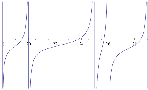
As may be seen from (3.21), the new eigenvalues interlace between the sequence 𝒩={n1<n2<…}\mathcal{N}=\{n_{1}<n_{2}<\dots\} of norms, see Figure 1. We may thus label the perturbed eigenvalues λk=λkϕ\lambda_{k}=\lambda_{k}^{\phi} so that

(3.23) n1<λ1<n2<λ2<⋯<nk<λk<nk+1<…n_{1}<\lambda_{1}<n_{2}<\lambda_{2}<\dots<n_{k}<\lambda_{k}<n_{k+1}<\dots
Refer to caption
Figure 1. A plot of the spectral function on the LHS of the eigenvalue equation (3.21) for the standard lattice ℒ=ℤ2\mathcal{L}={\mathbb{Z}}^{2}. The intersections of the plot with the xx-axis are the perturbed eigenvalues corresponding to ϕ=0\phi=0, alternating with the norms.

3.3. The density of states

The density of states of the perturbed eigenvalues depends strongly on the particular torus, that is on the lattice it determines.

For the standard lattice ℤ2{\mathbb{Z}}^{2}, a theorem of Landau [14] asserts that

(3.24) #⁡{n∈𝒩,n≤x}∼B​xlog⁡x,\#\{n\in\mathcal{N},n\leq x\}\sim B\frac{x}{\sqrt{\log x}},

where B=12∏(1−p−2)−1/2=0.764…B=\frac{1}{\sqrt{2}}\prod(1-p^{-2})^{-1/2}=0.764\dots, the product over primes p=3mod4p=3\bmod 4. Consequently we deduce a form of Weyl’s law for the perturbed spectrum Λϕ\Lambda_{\phi} of Δϕ,x0\Delta_{\phi,x_{0}} for the standard lattice:

(3.25) #⁡{λ∈Λϕ:λ≤x}∼B​xlog⁡x\#\{\lambda\in\Lambda_{\phi}:\lambda\leq x\}\sim B\frac{x}{\sqrt{\log x}}

In the irrational case, the multiplicities are typically 44, see (2.9). Then Weyl’s law in those cases would read as

(3.26) #⁡{λ∈Λϕ:λ≤x}∼π4​x\#\{\lambda\in\Lambda_{\phi}:\lambda\leq x\}\sim\frac{\pi}{4}x

4. The norm of GλG_{\lambda}

We will need a lower bound on the L2L^{2}-norm of the Green’s function GλG_{\lambda}. We are able to get a good bound for a sub-sequence of density one. To define this subsequence, we recall our discussion of the gaps between consecutive norms.

According to Lemma 2.1, for almost all kk we have

(4.1) nk+1−nk≪nko⁡(1)n_{k+1}-n_{k}\ll n_{k}^{o(1)}

We define the set Λg⊂Λ\Lambda_{g}\subset\Lambda of eigenvalues λk\lambda_{k} (using the labeling (3.23)) so that (4.1) holds:

(4.2) Λg={λk∈Λ:nk+1−nk≪λko⁡(1)}\Lambda_{g}=\{\lambda_{k}\in\Lambda:n_{k+1}-n_{k}\ll\lambda_{k}^{o(1)}\}

By the discussion above, this is a set of density one in Λ\Lambda (and conjecturally all of Λ\Lambda).

Lemma 4.1.

For λ∈Λg\lambda\in\Lambda_{g} (i.e. for almost all λ\lambda), we have

(4.3) ‖Gλ‖≫1λo⁡(1)||G_{\lambda}||\gg\frac{1}{\lambda^{o(1)}}
Proof.

Let nk=nk​(λ)n_{k}=n_{k}(\lambda), nk+1=nk+1​(λ)n_{k+1}=n_{k+1}(\lambda) be consecutive norms so that nk<λ<nk+1n_{k}<\lambda<n_{k+1}. Then trivially

(4.4) ‖Gλ‖22≫∑n∈𝒩rℒ​(n)(n−λ)2≥1(nk−λ)2>1(nk+1−nk)2\left\|G_{\lambda}\right\|^{2}_{2}\gg\sum_{n\in\mathcal{N}}\frac{r_{\mathcal{L}}(n)}{(n-\lambda)^{2}}\geq\frac{1}{(n_{k}-\lambda)^{2}}>\frac{1}{(n_{k+1}-n_{k})^{2}}

Since for λ∈Λg\lambda\in\Lambda_{g} we know that nk+1−nk≪nko⁡(1)n_{k+1}-n_{k}\ll n_{k}^{o(1)}, (4.3) follows. ∎

It is natural to conjecture that (4.3) holds for all λ\lambda.

5. Truncation

For L>0L>0 let A⁡(λ,L)A(\lambda,L) be the set of lattice points in the annulus λ−L<|x|2<λ+L\lambda-L<|x|^{2}<\lambda+L:

(5.1) A⁡(λ,L)={ξ∈ℒ:||ξ|2−λ|<L}A(\lambda,L)=\{\xi\in\mathcal{L}:\left||\xi|^{2}-\lambda\right|<L\}

We denote the truncated Green’s function by

(5.2) Gλ,L(x,x0)=−14​π2∑ξ∈A⁡(λ,L)exp⁡(i​ξ⋅(x−x0))|ξ|2−λ.G_{\lambda,L}(x,x_{0})=-\frac{1}{4\pi^{2}}\sum_{\xi\in A(\lambda,L)}\frac{\exp({\mathrm{i}}\xi\cdot(x-x_{0}))}{|\xi|^{2}-\lambda}.

Let gλg_{\lambda} and gλ,Lg_{\lambda,L} be the L2L^{2}-normalized Green’s function and its truncation:

(5.3) gλ=Gλ‖Gλ‖,gλ,L=Gλ,L‖Gλ,L‖g_{\lambda}=\frac{G_{\lambda}}{||G_{\lambda}||},\quad g_{\lambda,L}=\frac{G_{\lambda,L}}{||G_{\lambda,L}||}

We have the following approximation.

Lemma 5.1.

Let L=λδL=\lambda^{\delta}, θ/2<δ<1\theta/2<\delta<1. As λ→∞\lambda\to\infty along Λg\Lambda_{g},

‖gλ−gλ,L‖2→0.\left\|g_{\lambda}-g_{\lambda,L}\right\|_{2}\to 0.
Proof.

Note that

(5.4) ‖Gλ‖Gλ‖2−Gλ,L‖Gλ,L‖2‖2≤‖Gλ−Gλ,L‖2‖Gλ‖2+‖Gλ,L‖2​|1‖Gλ‖2−1‖Gλ,L‖2|≤ 2​‖Gλ−Gλ,L‖2‖Gλ‖2.\begin{split}\left\|\frac{G_{\lambda}}{\left\|G_{\lambda}\right\|_{2}}-\frac{G_{\lambda,L}}{\left\|G_{\lambda,L}\right\|_{2}}\right\|_{2}\leq&\;\frac{\left\|G_{\lambda}-G_{\lambda,L}\right\|_{2}}{\left\|G_{\lambda}\right\|_{2}}\\ &+\left\|G_{\lambda,L}\right\|_{2}\left|\frac{1}{\left\|G_{\lambda}\right\|_{2}}-\frac{1}{\left\|G_{\lambda,L}\right\|_{2}}\right|\\ \leq&\;2\,\frac{\left\|G_{\lambda}-G_{\lambda,L}\right\|_{2}}{\left\|G_{\lambda}\right\|_{2}}.\end{split}

We have

(5.5) ‖Gλ−Gλ,L‖22=116​π4​∑||ξ|2−λ|≥λδ1(|ξ|2−λ)2\left\|G_{\lambda}-G_{\lambda,L}\right\|_{2}^{2}=\frac{1}{16\pi^{4}}\sum_{||\xi|^{2}-\lambda|\geq\lambda^{\delta}}\frac{1}{(|\xi|^{2}-\lambda)^{2}}

We recall how to evaluate lattice sums using summation by parts:

Let n1<n2<…n_{1}<n_{2}<\dots be the set of norms, and

(5.6) N⁡(t)=∑nk≤trℒ​(nk)N(t)=\sum_{n_{k}\leq t}r_{\mathcal{L}}(n_{k})

Then for a smooth function f⁡(t)f(t) on ℝ{\mathbb{R}} we have

(5.7) ∑nA<|ξ|2≤nBf⁡(|ξ|2)=N⁡(nB)​f​(nB)−N⁡(nA)​f​(nA+1)−∫nA+1nBf′​(t)​N​(t)​𝑑t\sum_{n_{A}<|\xi|^{2}\leq n_{B}}f(|\xi|^{2})=N(n_{B})f(n_{B})-N(n_{A})f(n_{A+1})-\int_{n_{A+1}}^{n_{B}}f^{\prime}(t)N(t)dt

Now use the lattice count with remainder (2.3) to get

(5.8) ∑nA<|ξ|2≤nBf⁡(|ξ|2)=π​∫nA+1nBf⁡(t)​𝑑t+O⁡(nBθ​f​(nB)+nA+1θ​f​(nA))+O⁡(∫nA+1nB|f′​(t)|​tθ​dt)\sum_{n_{A}<|\xi|^{2}\leq n_{B}}f(|\xi|^{2})=\pi\int_{n_{A+1}}^{n_{B}}f(t)dt\\ +O(n_{B}^{\theta}f(n_{B})+n_{A+1}^{\theta}f(n_{A}))+O(\int_{n_{A+1}}^{n_{B}}|f^{\prime}(t)|t^{\theta}dt)

Applying (5.8) with f⁡(t)=1/(t−λ)2f(t)=1/(t-\lambda)^{2}, once with nA=n1n_{A}=n_{1} and nB≤λ−L<nB+1n_{B}\leq\lambda-L<n_{B+1} and then with nA−1<λ+L≤nA<nA+1n_{A-1}<\lambda+L\leq n_{A}<n_{A+1} and nB=∞n_{B}=\infty gives

(5.9) ‖Gλ−Gλ,L‖22≪1L+λθL2\left\|G_{\lambda}-G_{\lambda,L}\right\|_{2}^{2}\ll\frac{1}{L}+\frac{\lambda^{\theta}}{L^{2}}

Since for λ∈Λg\lambda\in\Lambda_{g} we have ‖Gλ‖2≫1/λo⁡(1)||G_{\lambda}||^{2}\gg 1/\lambda^{o(1)} by Lemma 4.1, we find

‖Gλ−GλL‖22‖Gλ‖22≪λo⁡(1)​(1L+λθL2)\frac{\left\|G_{\lambda}-G^{L}_{\lambda}\right\|_{2}^{2}}{\left\|G_{\lambda}\right\|_{2}^{2}}\ll\lambda^{o(1)}\left(\frac{1}{L}+\frac{\lambda^{\theta}}{L^{2}}\right)

which tends to zero if δ>θ/2\delta>\theta/2. ∎

Consequently we may study the matrix elements by replacing gλg_{\lambda} by the truncated version gλ,Lg_{\lambda,L}:

Lemma 5.2.

Let f∈C∞​(𝕋2)f\in C^{\infty}({\mathbb{T}}^{2}) and L=λδL=\lambda^{\delta}, θ/2<δ<1\theta/2<\delta<1. We have

|⟨f​gλ,gλ⟩−⟨f​gλ,L,gλ,L⟩|→0|\left\langle f\,g_{\lambda},g_{\lambda}\right\rangle-\left\langle f\,g_{\lambda,L},g_{\lambda,L}\right\rangle|\to 0

as λ→∞\lambda\to\infty along Λg\Lambda_{g}.

Proof.

Let f∈C∞​(𝕋2)f\in C^{\infty}({\mathbb{T}}^{2}). We define the multiplication operator Mf:L2​(𝕋2)→L2​(𝕋2)M_{f}:L^{2}({\mathbb{T}}^{2})\to L^{2}({\mathbb{T}}^{2}) by

Mf​(g)=f​g.M_{f}(g)=f\,g.

Since MfM_{f} is a continuous operator on L2​(𝕋2)L^{2}({\mathbb{T}}^{2}), we have that

‖gλ−gλ,L‖2→0\left\|g_{\lambda}-g_{\lambda,L}\right\|_{2}\to 0

for λ∈Λg\lambda\in\Lambda_{g} implies

‖Mf​(gλ−gλ,L)‖2→0\left\|M_{f}(g_{\lambda}-g_{\lambda,L})\right\|_{2}\to 0

and hence

|⟨Mf​gλ,gλ−gλ,L⟩|≤‖Mf‖∞​‖gλ−gλ,L‖→0.|\left\langle M_{f}\,g_{\lambda},g_{\lambda}-g_{\lambda,L}\right\rangle|\leq\left\|M_{f}\right\|_{\infty}\left\|g_{\lambda}-g_{\lambda,L}\right\|\to 0.

If we repeat this, where we switch gλg_{\lambda} and gλ,Lg_{\lambda,L}, we obtain

|⟨Mf​gλ,gλ⟩−⟨Mf​gλ,L,gλ,L⟩|→0.|\left\langle M_{f}g_{\lambda},g_{\lambda}\right\rangle-\left\langle M_{f}g_{\lambda,L},g_{\lambda,L}\right\rangle|\to 0.

∎

6. Exceptional eigenvalues and a Diophantine inequality

Fix a nonzero vector 0≠ζ∈ℒ0\neq\zeta\in\mathcal{L}, and δ∈(θ2,12−θ)\delta\in(\tfrac{\theta}{2},\tfrac{1}{2}-\theta) (such δ\delta exists because θ<1/3\theta<1/3). Let SζS_{\zeta} be the set of vectors satisfying

(6.1) Sζ={η∈ℒ:|⟨η,ζ⟩|≤|η|2​δ}S_{\zeta}=\{\eta\in\mathcal{L}:|\langle\eta,\zeta\rangle|\leq|\eta|^{2\delta}\}

We define a subset Λζ⊂Λ\Lambda_{\zeta}\subset\Lambda of eigenvalues

(6.2) Λζ={λ∈Λ:A⁡(λ,λδ)∩Sζ=∅}\Lambda_{\zeta}=\{\lambda\in\Lambda:A(\lambda,\lambda^{\delta})\cap S_{\zeta}=\emptyset\}

(recall that A⁡(λ,L)A(\lambda,L) are the lattice points η∈ℒ\eta\in\mathcal{L} in the annulus (5.1)). Our goal in this section is to show that

Proposition 6.1.

Λζ\Lambda_{\zeta} is a subset of density one in Λ\Lambda.

Proof.

Let

(6.3) Bζ=Λ\Λζ={λ∈Λ:A⁡(λ,λδ)∩Sζ≠∅}B_{\zeta}=\Lambda\backslash\Lambda_{\zeta}=\{\lambda\in\Lambda:A(\lambda,\lambda^{\delta})\cap S_{\zeta}\neq\emptyset\}

We will show that BζB_{\zeta} has density zero in the set Λ\Lambda of all perturbed eigenvalues, in fact

(6.4) #⁡{λ∈Bζ:λ≤X}≪X1−δ′|ζ|\#\{\lambda\in B_{\zeta}:\lambda\leq X\}\ll\frac{X^{1-\delta^{\prime}}}{|\zeta|}

for δ′=1/2−θ−δ>0\delta^{\prime}=1/2-\theta-\delta>0.

We first show that

Lemma 6.2.
(6.5) #⁡{η∈Sζ:|η|2≤X}≪X12+δ|ζ|\#\{\eta\in S_{\zeta}:|\eta|^{2}\leq X\}\ll\frac{X^{\frac{1}{2}+\delta}}{|\zeta|}
Proof.

Introduce cartesian coordinates with one of the axes in the direction of the vector ζ\zeta by writing every x∈ℝ2x\in{\mathbb{R}}^{2} as

(6.6) x=u​ζ|ζ|+v​ζ⟂|ζ⟂|x=u\frac{\zeta}{|\zeta|}+v\frac{\zeta^{\perp}}{|\zeta^{\perp}|}

where if ζ=(a​p,qa)\zeta=(ap,\frac{q}{a}) then ζ⟂=(−qa,p​a)\zeta^{\perp}=(-\frac{q}{a},pa) is a vector orthogonal to ζ\zeta. In these coordinates,

(6.7) ⟨x,ζ⟩=u​|ζ|,|x|2=u2+v2\langle x,\zeta\rangle=u|\zeta|\;,\quad|x|^{2}=u^{2}+v^{2}

and our set of lattice points is thus contained in the rectangle

(6.8) ℛ={uζ|ζ|+vζ⟂|ζ⟂|:|u|≤Xδ|ζ|,|v|≤X1/2}\mathcal{R}=\{u\frac{\zeta}{|\zeta|}+v\frac{\zeta^{\perp}}{|\zeta^{\perp}|}:|u|\leq\frac{X^{\delta}}{|\zeta|},\quad|v|\leq X^{1/2}\}

Now estimating the number of lattice points in a rectangle is a simple matter: Putting a fundamental domain ℱ={(ax,y/a):0≤x,y≤1}\mathcal{F}=\{(ax,y/a):0\leq x,y\leq 1\} for the lattice (which has unit area for the case at hand) centered around each lattice point in ℛ\mathcal{R}, we get a figure whose area is the number of lattice points in question, and which is contained in a slightly bigger rectangle whose dimensions are expanded by the diameter dℒ=a2+1/a2d_{\mathcal{L}}=\sqrt{a^{2}+1/a^{2}} of ℱ\mathcal{F}:

(6.9) ℛ+={uζ|ζ|+vζ⟂|ζ⟂|:|u|≤Xδ|ζ|+dℒ,|v|≤X1/2+dℒ}\mathcal{R}^{+}=\{u\frac{\zeta}{|\zeta|}+v\frac{\zeta^{\perp}}{|\zeta^{\perp}|}:|u|\leq\frac{X^{\delta}}{|\zeta|}+d_{\mathcal{L}},\quad|v|\leq X^{1/2}+d_{\mathcal{L}}\}

Thus we see that #​ℒ∩ℛ\#\mathcal{L}\cap\mathcal{R} is bounded by the area of ℛ+\mathcal{R}^{+}, which is:

(6.10) area⁡ℛ+=2​(Xδ|ζ|+dℒ)×2​(X1/2+dℒ)=4​X1/2+δ|ζ|+Oℒ​(X1/2)\operatorname{area}\mathcal{R}^{+}=2(\frac{X^{\delta}}{|\zeta|}+d_{\mathcal{L}})\times 2(X^{1/2}+d_{\mathcal{L}})=\frac{4X^{1/2+\delta}}{|\zeta|}+O_{\mathcal{L}}(X^{1/2})

Therefore

(6.11) #⁡{η∈Sζ:|η|2≤X}≤area⁡ℛ+=4​X1/2+δ|ζ|+Oℒ​(X1/2)\#\{\eta\in S_{\zeta}:|\eta|^{2}\leq X\}\leq\operatorname{area}\mathcal{R}^{+}=\frac{4X^{1/2+\delta}}{|\zeta|}+O_{\mathcal{L}}(X^{1/2})

as claimed. ∎

Next we define 𝒩ζ⊂𝒩\mathcal{N}_{\zeta}\subset\mathcal{N} to be the set of norms |η|2|\eta|^{2} of η∈Sζ\eta\in S_{\zeta}, without multiplicities. We clearly have

(6.12) #⁡{n∈𝒩ζ:n≤X}≤#⁡{η∈Sζ:|η|2≤X}≪X1/2+δ|ζ|\#\{n\in\mathcal{N}_{\zeta}:n\leq X\}\leq\#\{\eta\in S_{\zeta}:|\eta|^{2}\leq X\}\ll\frac{X^{1/2+\delta}}{|\zeta|}

by Lemma 6.2.

We have a map

(6.13) ι:Bζ→𝒩ζ\iota:B_{\zeta}\to\mathcal{N}_{\zeta}

defined by ι⁡(λ)\iota(\lambda) being the closest n∈𝒩ζn\in\mathcal{N}_{\zeta} to λ\lambda; if there are two such elements, i.e. n−<λ<n+n_{-}<\lambda<n_{+} with n±∈𝒩ζn_{\pm}\in\mathcal{N}_{\zeta} and n+−λ=λ−n−n_{+}-\lambda=\lambda-n_{-}, then set ι⁡(λ)=n+\iota(\lambda)=n_{+}. Thus we get a well defined map, whose fibers satisfy

ι−1(n)⊆{λ∈Λ:∃η∈Sζ∩A(λ,λδ),|η|2=n}⊆Λ∩[n−2nδ,n+2nδ]\iota^{-1}(n)\subseteq\{\lambda\in\Lambda:\exists\eta\in S_{\zeta}\cap A(\lambda,\lambda^{\delta}),|\eta|^{2}=n\}\subseteq\Lambda\cap[n-2n^{\delta},n+2n^{\delta}]

for n≫1n\gg 1.

Since Λ\Lambda is interlaced between the norms 𝒩\mathcal{N}, we have

(6.14) #​Λ∩[n−2​nδ,n+2​nδ]≪∑n−3​nδ<m<n+3​nδrℒ​(m)=#​A​(n,3​nδ)\#\Lambda\cap[n-2n^{\delta},n+2n^{\delta}]\ll\sum_{n-3n^{\delta}<m<n+3n^{\delta}}r_{\mathcal{L}}(m)=\#A(n,3n^{\delta})

which is the number of lattice points in an annulus. By (2.6),

(6.15) #​A​(n,3​nδ)≪nδ+nθ\#A(n,3n^{\delta})\ll n^{\delta}+n^{\theta}

and hence (since δ<θ\delta<\theta)

(6.16) #​ι−1​(n)≪nθ\#\iota^{-1}(n)\ll n^{\theta}

We thus find

(6.17) #⁡{λ∈Bζ:λ≤X}=∑n∈𝒩ζn≤X#​ι−1​(n)≪Xθ​#​{n∈𝒩ζ:n≤X}≪X1/2+δ+θ|ζ|\begin{split}\#\{\lambda\in B_{\zeta}:\lambda\leq X\}&=\sum_{\begin{subarray}{c}n\in\mathcal{N}_{\zeta}\\ n\leq X\end{subarray}}\#\iota^{-1}(n)\\ &\ll X^{\theta}\#\{n\in\mathcal{N}_{\zeta}:n\leq X\}\ll\frac{X^{1/2+\delta+\theta}}{|\zeta|}\end{split}

That is

(6.18) #⁡{λ∈Bζ:λ≤X}≪X1−δ′|ζ|\#\{\lambda\in B_{\zeta}:\lambda\leq X\}\ll\frac{X^{1-\delta^{\prime}}}{|\zeta|}

with δ′=1/2−θ−δ>0\delta^{\prime}=1/2-\theta-\delta>0. ∎

7. Proof of Theorem 1.1

7.1. Fixed observables

Fix a nonzero vector ζ∈ℒ\zeta\in\mathcal{L} and recall the definition (6.2), (4.2) of the sets of eigenvalues Λζ\Lambda_{\zeta} and Λg\Lambda_{g}; both are of density one in Λ\Lambda and thus

(7.1) Λg,ζ:=Λg∩Λζ\Lambda_{g,\zeta}:=\Lambda_{g}\cap\Lambda_{\zeta}

is still a set of density one in Λ\Lambda.

We will show that ⟨eζ​gλ,gλ⟩→0\langle e_{\zeta}g_{\lambda},g_{\lambda}\rangle\to 0 as λ→∞\lambda\to\infty along Λg,ζ\Lambda_{g,\zeta}. By Lemma 5.1 it suffices to show:

Proposition 7.1.

Take λ∈Λg,δ\lambda\in\Lambda_{g,\delta} and L=λδL=\lambda^{\delta}, δ∈(θ2,12−θ)\delta\in(\tfrac{\theta}{2},\tfrac{1}{2}-\theta). Fix nonzero ζ∈ℒ\zeta\in\mathcal{L}. As λ→0\lambda\to 0 while λ∈Λg,ζ\lambda\in\Lambda_{g,\zeta},

(7.2) ⟨eζ​gλ,L,gλ,L⟩→0\left\langle e_{\zeta}\,g_{\lambda,L},g_{\lambda,L}\right\rangle\to 0
Proof.

For ξ∈ℒ\xi\in\mathcal{L} and λ∈Λg,ζ\lambda\in\Lambda_{g,\zeta} define

c⁡(ξ)=1|ξ|2−λ.c(\xi)=\frac{1}{|\xi|^{2}-\lambda}.

The L2L^{2}-norm of the truncated Green’s function Gλ,LG_{\lambda,L} (L=λδL=\lambda^{\delta}) is given by

(7.3) ‖Gλ,L‖22=116​π4​∑ξ∈A⁡(λ,L)c​(ξ)2\left\|G_{\lambda,L}\right\|_{2}^{2}=\frac{1}{16\pi^{4}}\sum_{\xi\in A(\lambda,L)}c(\xi)^{2}

and hence

(7.4) ⟨eζ​Gλ,L,Gλ,L⟩=116​π4​∑ξ∈A⁡(λ,L)c⁡(ξ)​c​(ξ−ζ).\left\langle e_{\zeta}\,G_{\lambda,L},G_{\lambda,L}\right\rangle=\frac{1}{16\pi^{4}}\sum_{\xi\in A(\lambda,L)}c(\xi)c(\xi-\zeta)\;.

Cauchy-Schwarz gives

|⟨eζ​Gλ,L,Gλ,L⟩|2≤‖Gλ,L‖22​∑ξ∈A⁡(λ,L)c​(ξ−ζ)2.|\left\langle e_{\zeta}\,G_{\lambda,L},G_{\lambda,L}\right\rangle|^{2}\leq\left\|G_{\lambda,L}\right\|_{2}^{2}\,\sum_{\xi\in A(\lambda,L)}c(\xi-\zeta)^{2}.

Note that for λ∈Λζ,g\lambda\in\Lambda_{\zeta,g},

|c⁡(ξ−ζ)|≪1L.|c(\xi-\zeta)|\ll\frac{1}{L}.

Indeed

(7.5) |ξ−ζ|2−λ=|ξ|2−λ−2​⟨ξ,ζ⟩+|ζ|2|\xi-\zeta|^{2}-\lambda=|\xi|^{2}-\lambda-2\langle\xi,\zeta\rangle+|\zeta|^{2}

and since for λ∈Λζ\lambda\in\Lambda_{\zeta} and ξ∈A⁡(λ,L)\xi\in A(\lambda,L) we have |⟨ξ,ζ⟩|>|ξ|2​δ∼L|\langle\xi,\zeta\rangle|>|\xi|^{2\delta}\sim L we find that

(7.6) ||ξ−ζ|2−λ|≥2​L​(1+o⁡(1))−L−|ζ|2≫L\left||\xi-\zeta|^{2}-\lambda\right|\geq 2L(1+o(1))-L-|\zeta|^{2}\gg L

Using (2.6) gives the bound

(7.7) ∑ξ∈A⁡(λ,L)c​(ξ−ζ)2≪#​A​(λ,L)L2≪λθL2\sum_{\xi\in A(\lambda,L)}c(\xi-\zeta)^{2}\ll\frac{\#A(\lambda,L)}{L^{2}}\ll\frac{\lambda^{\theta}}{L^{2}}

(recall θ≥1/4\theta\geq 1/4) so that we find

(7.8) ⟨eζ​Gλ,L,Gλ,L⟩≪‖Gλ‖​λθ/2L\left\langle e_{\zeta}\,G_{\lambda,L},G_{\lambda,L}\right\rangle\ll||G_{\lambda}||\frac{\lambda^{\theta/2}}{L}

The lower bound ‖Gλ‖≫1/λo⁡(1)||G_{\lambda}||\gg 1/\lambda^{o(1)} of Lemma 4.1 implies

⟨eζ​gλ,L,gλ,L⟩=⟨eζ​Gλ,L,Gλ,L⟩‖Gλ,L‖22≪λθ/2+o⁡(1)L=λθ/2+o⁡(1)λδ\left\langle e_{\zeta}\,g_{\lambda,L},g_{\lambda,L}\right\rangle=\frac{\left\langle e_{\zeta}\,G_{\lambda,L},G_{\lambda,L}\right\rangle}{\left\|G_{\lambda,L}\right\|_{2}^{2}}\ll\frac{\lambda^{\theta/2+o(1)}}{L}=\frac{\lambda^{\theta/2+o(1)}}{\lambda^{\delta}}

for λ∈Λg,ζ\lambda\in\Lambda_{g,\zeta}, which tends to zero since δ>θ/2\delta>\theta/2. ∎

7.2. A diagonalization argument

We have shown that for each 0≠ζ∈ℒ0\neq\zeta\in\mathcal{L}, there is a density one subset Λg,ζ\Lambda_{g,\zeta} of eigenvalues so that ⟨eζ​gλ,gλ⟩→0\langle e_{\zeta}g_{\lambda},g_{\lambda}\rangle\to 0 as λ→∞\lambda\to\infty along Λg,ζ\Lambda_{g,\zeta}. It remains to see that there is a density one subset Λ∞⊂Λ\Lambda_{\infty}\subset\Lambda so that for every observable a∈C∞​(𝕋2)a\in C^{\infty}({\mathbb{T}}^{2}), we have

(7.9) ⟨a​gλ,gλ⟩→1area​(𝕋2)​∫𝕋2a⁡(x)​𝑑x\langle ag_{\lambda},g_{\lambda}\rangle\to\frac{1}{\mbox{area}({\mathbb{T}}^{2})}\int_{{\mathbb{T}}^{2}}a(x)dx

as λ→∞\lambda\to\infty along Λ∞\Lambda_{\infty}. We recall the argument, which can be found e.g. in [7]. For J≥1J\geq 1, let ΛJ⊂Λ\Lambda_{J}\subset\Lambda be of density one so that for all |ζ|≤J|\zeta|\leq J, ⟨eζ​gλ,gλ⟩→0\langle e_{\zeta}g_{\lambda},g_{\lambda}\rangle\to 0 as λ→∞\lambda\to\infty along Λg,ζ\Lambda_{g,\zeta}, and in particular for every trigonometric polynomial PJ​(x)=∑|ζ|≤Jpζ​eζ​(x)P_{J}(x)=\sum_{|\zeta|\leq J}p_{\zeta}e_{\zeta}(x) we have

(7.10) ⟨PJ​gλ,gλ⟩→1area​(𝕋2)​∫𝕋2PJ​(x)​𝑑x\langle P_{J}g_{\lambda},g_{\lambda}\rangle\to\frac{1}{\mbox{area}({\mathbb{T}}^{2})}\int_{{\mathbb{T}}^{2}}P_{J}(x)dx

We may assume that ΛJ+1⊆ΛJ\Lambda_{J+1}\subseteq\Lambda_{J} for each JJ. Now choose MJM_{J} so that for all X>MJX>M_{J},

(7.11) 1#⁡{λ∈Λ:λ≤X}#{λ∈ΛJ:λ≤X}≥1−12J\frac{1}{\#\{\lambda\in\Lambda:\lambda\leq X\}}\#\{\lambda\in\Lambda_{J}:\lambda\leq X\}\geq 1-\frac{1}{2^{J}}

and let Λ∞\Lambda_{\infty} be such that Λ∞∩[MJ,MJ+1]=ΛJ∩[MJ,MJ+1]\Lambda_{\infty}\cap[M_{J},M_{J+1}]=\Lambda_{J}\cap[M_{J},M_{J+1}] for all JJ. Then Λ∞∩[0,MJ+1]\Lambda_{\infty}\cap[0,M_{J+1}] contains ΛJ∩[0,MJ+1]\Lambda_{J}\cap[0,M_{J+1}] and therefore Λ∞\Lambda_{\infty} has density one in Λ\Lambda and (7.10) holds for λ∈Λ∞\lambda\in\Lambda_{\infty}. Since the trigonometric polynomials are dense in C∞​(𝕋2)C^{\infty}({\mathbb{T}}^{2}) in the uniform norm and the probability measures |gλ​(x)|2​d​x|g_{\lambda}(x)|^{2}dx are continuous with respect to this norm, we find that (7.9) holds.

Appendix A A rigorous description of the point scatterer

Denote by δx0\delta_{x_{0}} the Dirac distribution at x0∈𝕋2x_{0}\in\mathbb{T}^{2}. We are interested in solutions to the equation

(A.1) (Δ+λ)​f=δx0,f∈C∞​(𝕋2∖{x0}),‖f‖2=1(\Delta+\lambda)f=\delta_{x_{0}},\qquad f\in C^{\infty}(\mathbb{T}^{2}\setminus\{x_{0}\}),\;\left\|f\right\|_{2}=1

and its association with the eigenfunctions and eigenvalues of a family of self-adjoint operators. Consider the domain of C∞C^{\infty}-functions which vanish in a neighborhood of x0x_{0}

D0=C0∞​(𝕋2∖{x0})D_{0}=C^{\infty}_{0}(\mathbb{T}^{2}\setminus\{x_{0}\})

and denote −Δx0=−Δ|D0-\Delta_{x_{0}}=-\Delta|_{D_{0}}. The operators associated with equation (A.1) form the family of self-adjoint extensions of the positive symmetric operator −Δx0-\Delta_{x_{0}} (cf. [6], section 1, p. 277).

We make the following conventions in the definition of the Green’s function.

Definition 1.

Denote by σ⁡(−Δ)\sigma(-\Delta) the spectrum of −Δ-\Delta on C2​(𝕋2)C^{2}(\mathbb{T}^{2}). We define the Green’s function Gλ​(x,y)G_{\lambda}(x;y) at energy λ∈ℂ∖σ⁡(−Δ)\lambda\in{\mathbb{C}}\setminus\sigma(-\Delta) on 𝕋2\mathbb{T}^{2} as the integral kernel of the resolvent (Δ+λ)−1(\Delta+\lambda)^{-1}, that is

(A.2) (Δ+λ)−1​f​(y)=∫𝕋2Gλ​(x,y)​f​(x)​𝑑x.(\Delta+\lambda)^{-1}f(y)=\int_{\mathbb{T}^{2}}G_{\lambda}(x,y)f(x)dx.

In order to give a self-contained presentation of the theory of self-adjoint extensions, we briefly recall the standard definitions of the adjoint of an operator, symmetry and self-adjointness.

Definition 2.

Let HH be a Hilbert space and Dom⁡(B)⊂H\operatorname{Dom}(B)\subset H. Consider the operator B:Dom⁡(B)→HB:\operatorname{Dom}(B)\to H. We define

Dom(B∗)={y∈H∣∃a∈H:∀x∈Dom(B):⟨Bx,y⟩=⟨x,a⟩}\operatorname{Dom}(B^{*})=\{y\in H\mid\exists a\in H:\;\forall x\in\operatorname{Dom}(B):\;\left\langle Bx,y\right\rangle=\left\langle x,a\right\rangle\}

then we define the adjoint B∗B^{*} of BB as the map B∗:Dom⁡(B∗)→HB^{*}:\operatorname{Dom}(B^{*})\to H,

B∗​y=a.B^{*}y=a.

We call BB symmetric if

∀x,y∈Dom⁡(B):⟨B​x,y⟩=⟨x,B​y⟩.\forall x,y\in\operatorname{Dom}(B):\left\langle Bx,y\right\rangle=\left\langle x,By\right\rangle.

We call BB self-adjoint if BB is symmetric and

Dom⁡(B)=Dom⁡(B∗).\operatorname{Dom}(B)=\operatorname{Dom}(B^{*}).

We have the following well-known results from self-adjoint extension theory which we summarize briefly. Proofs can be found in [18], Chapter X.1. We will give the relevant references for each lemma.

Definition 3.

Let BB be a densely defined symmetric operator on a Hilbert space HH. Denote its adjoint by B∗B^{*}. Let η∈ℂ∖ℝ\eta\in{\mathbb{C}}\setminus{\mathbb{R}}. The deficiency spaces of BB at η\eta and η¯\bar{\eta} are defined as

(A.3) Dη​(B)=ker⁡{B∗−η},Dη¯​(B)=ker⁡{B∗−η¯}.D_{\eta}(B)=\ker\{B^{*}-\eta\},\qquad D_{\bar{\eta}}(B)=\ker\{B^{*}-\bar{\eta}\}.

We refer to the members of a basis of a deficiency space as deficiency elements.

The following lemma is proven as part of Theorem X.1, p. 136 in [18].

Lemma A.1.

As a function of η\eta, dimDη​(B)\dim D_{\eta}(B) is constant on the upper (lower) complex half-plane.

We proceed with the definition of the deficiency indices of a closed symmetric operator which indicate if the operator can be extended to a self-adjoint operator.

Definition 4.

If dimDη​(B)=m\dim D_{\eta}(B)=m and dimDη¯​(B)=n\dim D_{\bar{\eta}}(B)=n for nonnegative integers mm, nn, we say that the operator BB has deficiency indices (m,n)(m,n).

The following lemma is Corollary (a), p. 141 in [18].

Lemma A.2.

BB has deficiency indices (0,0)(0,0) if, and only if, BB is self-adjoint.

If the deficiency indices are nonzero and equal, then a family of self-adjoint extensions exists and can be constructed as follows. This lemma combines Theorem X.2, p. 140 and Corollary (b), p. 141 in [18].

Lemma A.3.

If a closed positive symmetric operator BB has deficiency indices (n,n)(n,n), n≥1n\geq 1, then for each unitary map U:Di​(B)→D−i​(B)U:D_{\mathrm{i}}(B)\to D_{-{\mathrm{i}}}(B) there is a self-adjoint extension BU:DU→HB_{U}:D_{U}\to H, where

(A.4) DU={f=g+h+U​h∣(g,h)∈Dom⁡(B)×Di​(B)}D_{U}=\{f=g+h+Uh\mid(g,h)\in\operatorname{Dom}(B)\times D_{{\mathrm{i}}}(B)\}

and BUB_{U} acts as follows

(A.5) BU​f=B​g+i​h−i​U​h.B_{U}f=Bg+{\mathrm{i}}h-{\mathrm{i}}Uh.

The operator BUB_{U} has deficiency indices (0,0)(0,0). Conversely, every self-adjoint extension of BB is of this form.

We apply Lemma A.3 to construct a one parameter family of self-adjoint extensions of the operator −Δx0-\Delta_{x_{0}}. Denote the domain of the closure of −Δx0-\Delta_{x_{0}} by D0~\tilde{D_{0}}.

Lemma A.4.

The operator −Δx0-\Delta_{x_{0}} has deficiency indices (1,1)(1,1). The corresponding deficiency elements are the Green’s functions Gi​(x,x0)G_{{\mathrm{i}}}(x,x_{0}), G−i​(x,x0)G_{-{\mathrm{i}}}(x,x_{0}).

The self-adjoint extensions of −Δx0-\Delta_{x_{0}} are given by the one parameter family

(A.6) −Δφ:Dφ→L2(𝕋2),φ∈(−π,π]-\Delta_{\varphi}:D_{\varphi}\to L^{2}(\mathbb{T}^{2}),\qquad\varphi\in(-\pi,\pi]

where

(A.7) Dφ={g+cGi+cei​φG−i:g∈D0~,c∈ℂ}D_{\varphi}=\{g+cG_{\mathrm{i}}+ce^{{\mathrm{i}}\varphi}G_{-{\mathrm{i}}}:g\in\tilde{D_{0}},c\in{\mathbb{C}}\}

and

(A.8) −Δφ​f=−Δ​g+c​i​Gi−c​ei​φ​i​G−i.-\Delta_{\varphi}f=-\Delta g+c{\mathrm{i}}G_{\mathrm{i}}-ce^{{\mathrm{i}}\varphi}{\mathrm{i}}G_{-{\mathrm{i}}}.
Proof.

By definition of the Green’s function we have that

(A.9) ker⁡{(Δx0)∗±i}=ℒ⁡{G±i}.\ker\{(\Delta_{x_{0}})^{*}\pm{\mathrm{i}}\}={\mathcal{L}}\{G_{\pm{\mathrm{i}}}\}.

Hence −Δx0-\Delta_{x_{0}} has deficiency indices (1,1)(1,1) and we may apply Lemma A.3 to obtain the result. ∎

Remark A.5.

Note that −Δπ-\Delta_{\pi} recovers the Laplacian on C∞​(𝕋2)C^{\infty}(\mathbb{T}^{2}).

Next we derive an equation for eigenvalues of the operator −Δφ-\Delta_{\varphi}, φ∈(−π,π)\varphi\in(-\pi,\pi).

Lemma A.6.

Let φ∈(−π,π)\varphi\in(-\pi,\pi). We have that λ∉σ⁡(−Δ)\lambda\notin\sigma(-\Delta) is an eigenvalue of −Δφ-\Delta_{\varphi} if, and only if,

(A.10) ∑ξ∈ℒ(1|ξ|2−λ−|ξ|2|ξ|4+1)=c0​tan⁡(φ/2),\sum_{\xi\in\mathcal{L}}\left(\frac{1}{|\xi|^{2}-\lambda}-\frac{|\xi|^{2}}{|\xi|^{4}+1}\right)=c_{0}\tan(\varphi/2),

where

c0=∑ξ∈ℒ1|ξ|4+1.c_{0}=\sum_{\xi\in\mathcal{L}}\frac{1}{|\xi|^{4}+1}.

The corresponding eigenfunction is a multiple of Gλ​(x,x0)G_{\lambda}(x;x_{0}).

Proof.

Let f∈Dφf\in D_{\varphi} and ‖f‖2=1\left\|f\right\|_{2}=1. Then ff must be of the form

(A.11) f=g+c​Gi+c​ei​φ​G−i,g∈D0,c∈ℂ.f=g+cG_{\mathrm{i}}+ce^{{\mathrm{i}}\varphi}G_{-{\mathrm{i}}},\qquad g\in D_{0},c\in{\mathbb{C}}.

Let us first assume that λ∉σ⁡(−Δ)\lambda\notin\sigma(-\Delta) is an eigenvalue of −Δφ-\Delta_{\varphi}. We have

(A.12) 0=(Δφ+λ)​f=(Δ+λ)​g+c⁡(λ−i)​Gi+c​ei​φ​(λ+i)​G−i.0=(\Delta_{\varphi}+\lambda)f=(\Delta+\lambda)g+c(\lambda-{\mathrm{i}})G_{\mathrm{i}}+ce^{{\mathrm{i}}\varphi}(\lambda+{\mathrm{i}})G_{-{\mathrm{i}}}.

We apply the resolvent (Δ+λ)−1(\Delta+\lambda)^{-1} to both sides to obtain

(A.13) 0=g+c​λ−iΔ+λ​Gi+c​ei​φ​λ+iΔ+λ​G−i.0=g+c\frac{\lambda-{\mathrm{i}}}{\Delta+\lambda}G_{\mathrm{i}}+ce^{{\mathrm{i}}\varphi}\frac{\lambda+{\mathrm{i}}}{\Delta+\lambda}G_{-{\mathrm{i}}}.

In view of the iterated resolvent identity

(A.14) (λ∓i)​1Δ+λ​1Δ±i=1Δ±i−1Δ+λ(\lambda\mp{\mathrm{i}})\frac{1}{\Delta+\lambda}\frac{1}{\Delta\pm{\mathrm{i}}}=\frac{1}{\Delta\pm{\mathrm{i}}}-\frac{1}{\Delta+\lambda}

we can rewrite equation (A.13) as

(A.15) 0=g⁡(x)+c⁡(Gi−Gλ)​(x,x0)+c​ei​φ​(G−i−Gλ)​(x,x0).0=g(x)+c(G_{\mathrm{i}}-G_{\lambda})(x,x_{0})+ce^{{\mathrm{i}}\varphi}(G_{-{\mathrm{i}}}-G_{\lambda})(x,x_{0}).

In particular

(A.16) f=g+c⁡(Gi+ei​ϕ​G−i)=c⁡(1+ei​ϕ)​Gλf=g+c(G_{\mathrm{i}}+e^{{\mathrm{i}}\phi}G_{-{\mathrm{i}}})=c(1+e^{{\mathrm{i}}\phi})G_{\lambda}

and so ff is a multiple of GλG_{\lambda}.

If we now take the limit x→x0x\to x_{0} on the r.h.s. of (A.15) we obtain

(A.17) 0=limx→x0(Gi−Gλ)​(x,x0)+ei​φ​limx→x0(G−i−Gλ)​(x,x0)0=\lim_{x\to x_{0}}(G_{\mathrm{i}}-G_{\lambda})(x,x_{0})+e^{{\mathrm{i}}\varphi}\lim_{x\to x_{0}}(G_{-{\mathrm{i}}}-G_{\lambda})(x,x_{0})

and note that λ∉σ⁡(−Δ)\lambda\notin\sigma(-\Delta) implies c≠0c\neq 0 so we may drop the constant. A simple rearrangement of this equation yields

(A.18) tan⁡(φ/2)​limx→x0Im⁡Gi​(x,x0)=limx→x0(Gλ−Re⁡Gi)​(x,x0).\tan(\varphi/2)\lim_{x\to x_{0}}\operatorname{Im}G_{\mathrm{i}}(x,x_{0})=\lim_{x\to x_{0}}(G_{\lambda}-\operatorname{Re}G_{\mathrm{i}})(x,x_{0}).

In order to obtain equation (A.10) we require the following L2L^{2}-identity for the Green’s function GλG_{\lambda} on 𝕋2\mathbb{T}^{2}

(A.19) Gλ(x,x0)=−14​π2∑ξ∈ℒexp⁡(i​ξ⋅(x−x0))|ξ|2−λ,x≠x0.G_{\lambda}(x,x_{0})=-\frac{1}{4\pi^{2}}\sum_{\xi\in\mathcal{L}}\frac{\exp({\mathrm{i}}\xi\cdot(x-x_{0}))}{|\xi|^{2}-\lambda},\qquad x\neq x_{0}.

We rewrite the r.h.s. of (A.18) as

(A.20) −14​π2∑ξ∈ℒe(ξ⋅(x−x0)){1|ξ|2−λ−Re1|ξ|2−i}=−14​π2∑ξ∈ℒe(ξ⋅(x−x0)){1|ξ|2−λ−|ξ|2|ξ|4+1}⟶x→x0−14​π2∑ξ∈ℒ{1|ξ|2−λ−|ξ|2|ξ|4+1}.\begin{split}&-\frac{1}{4\pi^{2}}\sum_{\xi\in\mathcal{L}}e(\xi\cdot(x-x_{0}))\left\{\frac{1}{|\xi|^{2}-\lambda}-\operatorname{Re}\frac{1}{|\xi|^{2}-{\mathrm{i}}}\right\}\\ =&-\frac{1}{4\pi^{2}}\sum_{\xi\in\mathcal{L}}e(\xi\cdot(x-x_{0}))\left\{\frac{1}{|\xi|^{2}-\lambda}-\frac{|\xi|^{2}}{|\xi|^{4}+1}\right\}\\ &\stackrel{{\scriptstyle x\to x_{0}}}{{\longrightarrow}}-\frac{1}{4\pi^{2}}\sum_{\xi\in\mathcal{L}}\left\{\frac{1}{|\xi|^{2}-\lambda}-\frac{|\xi|^{2}}{|\xi|^{4}+1}\right\}.\end{split}

Finally, note that

limx→x0ImGi(x,x0)=−14​π2∑ξ∈ℒ1|ξ|4+1.\lim_{x\to x_{0}}\operatorname{Im}G_{\mathrm{i}}(x,x_{0})=-\frac{1}{4\pi^{2}}\sum_{\xi\in\mathcal{L}}\frac{1}{|\xi|^{4}+1}.

To see the reverse implication assume that λ\lambda solves equation (A.17), a rearrangement of equation (A.10). The r.h.s. of equation (A.17) has singularities at points which are in σ⁡(−Δ)\sigma(-\Delta), hence λ∉σ⁡(−Δ)\lambda\notin\sigma(-\Delta). We define

fλ​(x)=(Gλ−Gi)​(x,x0)+ei​φ​(Gλ−G−i)​(x,x0)f_{\lambda}(x)=(G_{\lambda}-G_{\mathrm{i}})(x,x_{0})+e^{{\mathrm{i}}\varphi}(G_{\lambda}-G_{-{\mathrm{i}}})(x,x_{0})

and observe that

(A.21) (1+ei​φ)​Gλ=fλ+Gi+ei​φ​G−i∈Dφ(1+e^{{\mathrm{i}}\varphi})G_{\lambda}=f_{\lambda}+G_{{\mathrm{i}}}+e^{{\mathrm{i}}\varphi}G_{-{\mathrm{i}}}\in D_{\varphi}

because equation (A.17) implies fλ​(x0)=0f_{\lambda}(x_{0})=0. The iterated resolvent identity (A.14) implies

(A.22) (Δφ+λ)​fλ=(Δ+λ)​fλ=−(λ−i)​Gi−(λ+i)​Gi(\Delta_{\varphi}+\lambda)f_{\lambda}=(\Delta+\lambda)f_{\lambda}=-(\lambda-{\mathrm{i}})G_{\mathrm{i}}-(\lambda+{\mathrm{i}})G_{\mathrm{i}}

and by the definition of the operator Δφ\Delta_{\varphi} we have

(A.23) (1+ei​φ)​(Δφ+λ)​Gλ=(Δ+λ)​fλ+(λ−i)​Gi+(λ+i)​G−i=0.(1+e^{{\mathrm{i}}\varphi})(\Delta_{\varphi}+\lambda)G_{\lambda}=(\Delta+\lambda)f_{\lambda}+(\lambda-{\mathrm{i}})G_{\mathrm{i}}+(\lambda+{\mathrm{i}})G_{-{\mathrm{i}}}=0.

This concludes the proof. ∎

References

  • [1] R. P. Bambah and S. Chowla. On numbers which can be expressed as a sum of two squares. Proc. Nat. Inst. Sci. India, 13, 101–103 (1947).
  • [2] G. Berkolaiko, J. P. Keating and B. Winn. Intermediate wave functions statistics, Phys. Rev. Lett. 91, 134103 (2003).
  • [3] E. Bogomolny, U. Gerland and C. Schmit. Singular statistics. Phys. Rev. E (3) 63 (2001), no. 3, part 2, 036206.
  • [4] E. Bogomolny, O. Giraud and C. Schmit. Nearest-neighbor distribution for singular billiards. Phys. Rev. E (3) 65 (2002), no. 5, 056214.
  • [5] T. Shigehara and Taksu Cheon, Wave chaos in quantum billiards with a small but finite-size scatterer. Phys. Rev. E 54, 1321–1331 (1996).
  • [6] Y. Colin de Verdière. Pseudo-laplaciens I. Annales de l’Institut Fourier, tome 32, no. 3, 275-286, 1982.
  • [7] Y. Colin de Verdière Ergodicité et fonctions propres du laplacien. Comm. Math. Phys. 102 (1985), no. 3, 497–502.
  • [8] D. A. Hejhal. Some observations concerning eigenvalues of the Laplacian and Dirichlet L-series. Recent progress in analytic number theory, Symp. Durham 1979, Vol. 2, 95-110 (1981).
  • [9] M. N  Huxley, Exponential sums and lattice points. III. Proc. London Math. Soc. (3) 87 (2003), no. 3, 591–609.
  • [10] D. Jakobson. Quantum limits on flat tori. Ann. of Math. (2) 145 (1997), 235–266.
  • [11] J. P. Keating, J. Marklof and B. Winn. Localized eigenfunctions in S̆eba billiards. J. Math. Phys. 51 (2010), no. 6, 062101.
  • [12] S. Kerckhoff, H. Masur and J. Smillie, Ergodicity of billiard flows and quadratic differentials. Ann. of Math. (2) 124 (1986), no. 2, 293–311.
  • [13] R. de L.  Kronig and W. G. Penney, Quantum Mechanics of Electrons in Crystal Lattices. Proceedings of the Royal Society of London. Series A, Vol. 130, No. 814 (Feb. 3, 1931), pp. 499–513.
  • [14] E. Landau, Über die Einteilung der positiven ganzen Zahlen in vier Klassen nach der Mindeszahl der zu ihrer additiven Zusammensetzung erforderlichen Quadrate. Arch. Math. Phys. 13, 305–312, 1908.
  • [15] J. Marklof and Z. Rudnick, Almost all eigenfunctions of a rational polygon are uniformly distributed. J. of Spectral Theory. 2 (2012), 107–113.
  • [16] F. Oravecz, Z. Rudnick and I. Wigman, The Leray measure of nodal sets for random eigenfunctions on the torus, Annales de l’Institut Fourier 58 (1), (2008), 299–335.
  • [17] S. Rahav and S. Fishman. Spectral statistics of rectangular billiards with localized perturbations. Nonlinearity 15 (2002), no. 5, 1541–1594.
  • [18] M. Reed and B. Simon. Methods of Modern Mathematical Physics, Vol. 2: Fourier Analysis and Self-Adjointness. Academic Press, London, 1975.
  • [19] P. S̆eba. Wave Chaos in Singular Quantum Billiard. Phys. Rev. Letters, Vol. 64, No. 16, 1855-58, 1990.
  • [20] T. Shigehara, Conditions for the appearance of wave chaos in quantum singular systems with a pointlike scatterer. Phys. Rev. E 50, 4357–4370 (1994).
  • [21] A. Snirel’man Ergodic properties of eigenfunctions. Uspekhi Mat. Nauk 29, no. 6 (180), 181–182, 1974
  • [22] J. G . van der Corput, Neue zahlentheoretische Abschätzungen. Math. Ann. 89 (1923), no. 3–4, 215–254.
  • [23] S. Zelditch. Uniform distribution of eigenfunctions on compact hyperbolic surfaces. Duke Math. J. 55, no. 4, 919-941, 1987.
  • [24] S. Zelditch and M. Zworski, Ergodicity of eigenfunctions for ergodic billiards. Comm. Math. Phys. 175, 673–682, (1996).