Strategy of Competition between Two Groups based on a Contrarian Opinion Model
Abstract
We introduce a contrarian opinion (CO) model in which a fraction of contrarians within a group holds a strong opinion opposite to the opinion held by the rest of the group. At the initial stage, stable clusters of two opinions, and exist. Then we introduce contrarians which hold a strong opinion into the opinion group. Through their interactions, the contrarians are able to decrease the size of the largest opinion cluster, and even destroy it. We see this kind of method in operation, e.g when companies send free new products to potential customers in order to convince them to adopt the product and influence others. We study the CO model, using two different strategies, on both Erdös-Rényi and scale-free networks. In strategy I, the contrarians are positioned at random. In strategy II, the contrarians are chosen to be the highest degrees nodes. We find that for both strategies the size of the largest cluster decreases to zero as increases as in a phase transition. At a critical threshold value the system undergoes a second-order phase transition that belongs to the same universality class of mean field percolation. We find that even for an Erdös-Rényi type model, where the degrees of the nodes are not so distinct, strategy II is significantly more effctive in reducing the size of the largest opinion cluster and, at very small values of , the largest opinion cluster is destroyed.
pacs
89.75.Hc, 89.65.-s, 64.60.-i, 89.75.DaI Introduction
Competition between two groups or among a larger number of groups is ubiquitous in business and politics: the decades-long battle between the Mac and the PC in the computer industry, between Procter & Gamble and Unilever in the personal products industry, among all major international and local banks in the financial market, and among politicians and interest groups in the world of governance. All competitors want to increase the number of their supporters and thus increase their chances of success. In gathering supporters, competitors put much effort into persuading skeptics and those opponents who may actually be potential supporters. This kind of activity is normally modeled as a dynamic process on a complex network in which the nodes are the agents and the links are the interactions between agents. The goal of these models is to understand how an initially disordered configuration can become an ordered configuration through the interaction between agents. In the context of social science, order means agreement and disorder means disagreement [1, 2]. Most of these models—e.g., the Sznajd model [3], the voter model [4, 5], the majority rule model [6, 7], and the social impact model [8, 9]—are based on two-state spin systems which tend to reduce the variability of the initial state and lead to a consensus state in which all the agents share the same opinion. However this consensus state is not very realistic, since in many real competitions there are always at least two groups that co-exist at the same time.
Recently a non-consensus opinion (NCO) model [10] was developed, where two opinions and compete and reach a non-consensus stable state. At each time step each node adopts the opinion of the majority in its “neighborhood,” which consists of its nearest neighbors and itself. When there is a tie, the node does not change its state. Considering also the node’s own opinion leads to the non-consensus state. The dynamics are such that a steady state in which opinions and coexist is quickly reached. It was conjectured, and supported by intensive simulations [10], that the NCO model in complex networks belongs to the same universality class as percolation [10, 12, 11].
Here we test how competition strategies are affected when “contrarians” are introduced. Contrarians are agents who hold a strong opinion that is opposition to an opinion held by the rest of the group, and are not influenced by their opinion but can influence them. We develop a spin-type contrarian opinion (CO) model in which contrarian agents are introduced into the steady state of the NCO model. The goal of the contrarians is to change the opinions of the current supporters of the rival group [13]. We see this strategy in operation, for example, when companies send free new products to potential customers in order to convince them to adopt the product and encourage their friends to do the same. We can observe it also in political campaigns when candidates “bribe” voters by offering favors. The questions we ask in our model are as follows. Do these free products and bribes work and how? Who are the best individuals to chose as contrarians in order to make most impact on opinion change.
In this paper we introduce, into group , a fraction of contrarians, which are defined to be agents that hold a strong opinion, who will influence those who hold the opinion to change their opinion to . We study two different strategies of introducing contrarians, (I) random choosing of contrarians, and (II) targeted. We study these strategies on two types of networks, Erdös-Rényi (ER) [14] and scale free (SF) [15]. We find, for both strategies, that the relative size of the largest cluster in state undergoes a second order phase transition at a critical fraction of contrarians . Moreover we find that, for both networks analyzed here, the targeted strategy is much more efficient than the random strategy. Our results indicate that the observed second order phase transition can be mapped into mean field percolation.
II The CO Model
In the NCO model[10], initially, a fraction of agents with opinions and with opinions are selected at random. At each time step, each network node adopts the majority opinion based on the opinions of its neighbors and itself. All updates are performed simultaneously at each time step until a steady state is reached in which both opinions coexist, which occurs for above a critical threshold .
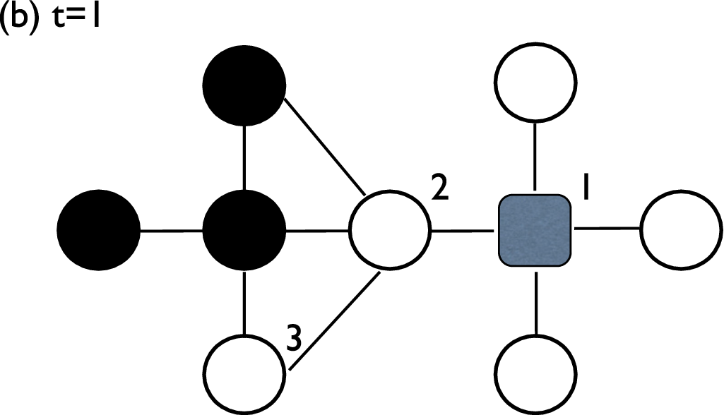
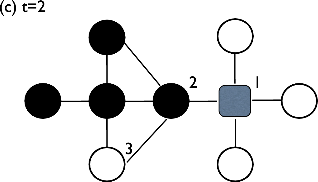
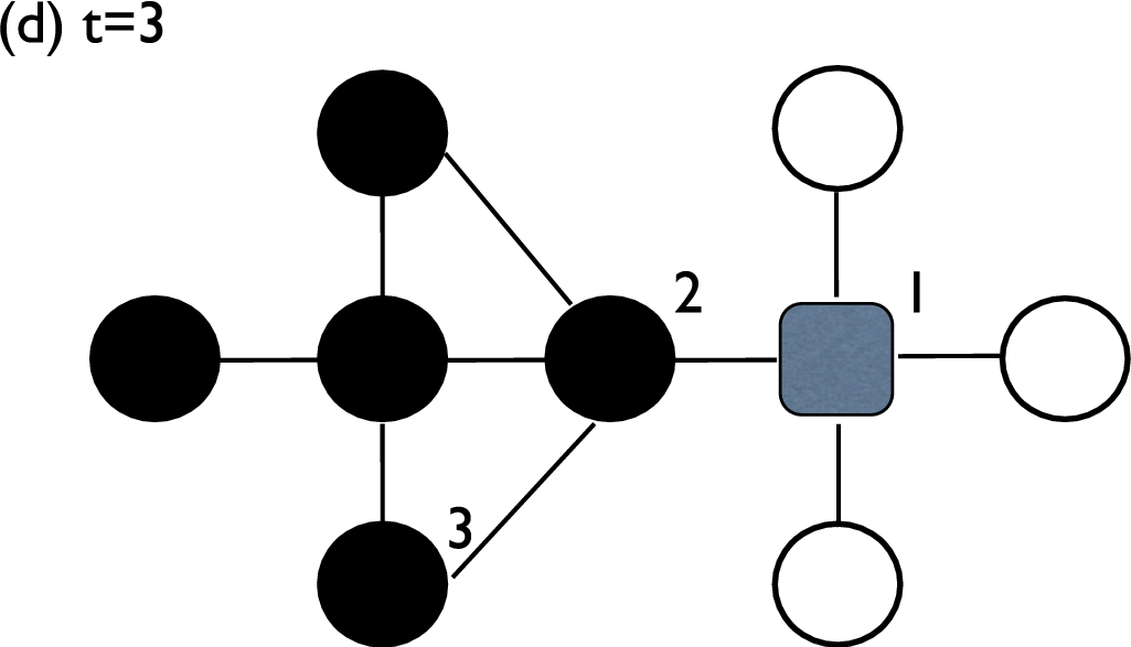
In our CO model, the initial state is the final state of the NCO model. Above we have stable clusters of both or opinions in a network of agents. We choose, initially, a fraction of opinion agents that are changed into opinion agents and so become contrarians. By contrarian we mean that, they will never change their opinion but they can influence others. Then we use again the NCO dynamics to reach a new steady state. In the new steady state the agents form again clusters of two opposite opinions above a certain threshold that now depends on . Because of the contrarians of type , the clusters become smaller and the clusters increase. In Fig. 1 we show a schematic plot of the dynamics of the CO model.
We use both random and targeted strategies to choose a fraction of agents that flip into state , and we analyze the results on ER and SF networks. In strategy I we randomly choose a fraction of A agents, and in strategy II we choose the top percent of the highest degree agents, to become contrarians. Notice that the contrarians act as a quenched disorder in the network [16, 11].
III Simulation Results
We perform simulations of the CO model in complex networks, on both ER and SF networks. ER networks are characterized by a Poisson degree distribution with , where is the degree of a node and is the average degree. In SF networks the degree distribution is given by , for , where is the smallest degree, is the degree cutoff and is the exponent characterizing the broadness of the distribution. In all our simulations we use the natural cutoff, which is controlled by [17]. We performed all the simulations for network realizations.
III.1 CO model on ER networks
We denote by the size of the largest cluster in the steady state. We study the effect of the contrarians. In Fig. 2 we plot as a function of for different values of for ER networks under both random and targeted strategies. The plot shows that there exists a critical value that depends on , below which approaches zero. As increases, the largest cluster becomes significantly smaller as well as less robust, as can been seen from the shift of to the larger value. In the inset of Fig. 2, we plot the size of the second largest cluster, , as a function of for different values of . shows a sharp peak characteristic of a second order phase transition, where is the order parameter and is the control parameter. Above a certain value of , the phase transition does not occur because, above , the average connectivity of the nodes decreases dramatically, the networks break into small clusters and no giant component of opinion appears. In Fig. 3 we show, for both strategies, the average degree of the opinion agents as a function of for different values of . As shown in [10] for , has a significant increase above where the nodes with opinion are majority. This is because when these nodes are in the minority group, they have a small average connectivity since the minority group doesn’t include high degree nodes. This process is analogous to targeted removing of the high degree nodes. Only when they become majority nodes, close to , the original connectivity of the full network is recovered. However, as increases, we never reach the original average degree of the full network because increasing is equivalent to increasing the quenched disorder. It is known that for ER networks the transition is lost when [14]. As we can see from the plots, for (strategy I) and (strategy II), drops below , and then the giant component cannot be sustained.
The loss of robustness is significantly more pronounced in the targeted strategy compared to the random strategy, as seen in Fig. 2(c), where we plot as a function of for both strategies. From this plot we can see that the targeted strategy is significantly more efficient to annihilate the opinion clusters than the random strategy. For example, for , the network is 25% less robust in the targeted strategy compared to the random one. The reason is that the initial state of our model is the final state of the NCO model, which above its threshold has clusters of nodes of all sizes. Thus under the random strategy we select nodes at random that are mainly in small clusters. Under the targeted strategy the selection of contrarians from the nodes of highest degree places them mainly in the largest initial cluster where they can influence more than if they were isolated in smaller clusters, as in the random strategy. The high degree nodes shorten the distances between all the pairs of nodes in a cluster, which allows them to interact more easily. Also, because they have many neighbors, they can influence the opinions of other nodes more efficiently.
In order to verify the above arguments, we compute, for our initial condition () before adding the contrarians, the degree distribution of nodes inside and outside the largest cluster. In Fig. 4(a) we plot the degree distributions of nodes inside and outside the largest cluster for three different values of above the threshold of the NCO model. Notice that the nodes outside the largest cluster have a degree distribution with a high probability of low connectivity. The probability of low connectivity increases as increases, and thus under a targeted strategy the nodes in those small clusters are almost never designated as contrarians. Thus nodes in the largest component are more likely to be selected under a targeted strategy than under a random one.
In order to further test our assumption, we compute the fraction , defined as the ratio of the number of nodes with degree in the largest cluster and the total number of nodes in all the clusters with the same degree. When , all the nodes with degree are in the largest cluster. In Fig. 4(b), we plot as a function of for different values of . As increases, we see that is faster for increasing because the larger is, the larger will be. Thus the highest degree nodes belong to the largest cluster and the lower degree nodes are less likely to be in the largest cluster. This explains why a targeted strategy is significantly more efficient than a random one.
Because is our main parameter, we next investigate the behavior of the system as a function of for different values of . In Fig. 5 we plot as a function of for fixed for ER networks under both strategies. From the plot we can see that is more robust as is larger, and the behavior of the curve is again characteristic of a second order phase transition. However this curve seems to be smoother than the transition found above (see Fig. 2) with as the control parameter.
In the inset of Fig. 5 (a) we plot the first derivative of with respect to for two different system sizes for . We can see a jump that becomes sharper as the system size increases. We find the same behavior for other values of above the threshold. In Figs. 6 (a) and 6 (b) we show and the first derivative of with respect to for and for different values of . We find that the peak of and the jump of the derivative of occurs at the same value of . This behavior is characteristic of a second order phase transition, where the peak of indicates the position of the threshold . In Fig. 6(c) we plot the critical threshold as a function of for both strategies. Comparing the two strategies for the same value of , strategy II always has the smaller . This demonstrates again that strategy II is better because a very small fraction of is enough to destroy the opinion clusters.
Next, we present results indicating that the CO model is in the same universality class as regular percolation. Percolation in random networks (e.g, ER)[12, 11, 18] predicts that at criticality the cluster size distribution of finite clusters with . In Fig. 7 we plot for both random and targeted strategies as a function of for finite clusters at criticality. As we can see for both strategies, . Moreover, from we calculate the exponent , which represents how the mean finite size diverges with distance to criticality (not shown here), from which we obtain , as in mean field percolation. The values of the two exponents we obtain strongly indicate that our CO model in ER networks is in the same universality class as mean field percolation in complex networks below [19].
III.2 CO model on SF networks
Many real social networks are not ER, but instead possess a SF degree distribution. It is well known that dynamic processes in SF networks propagate significantly more efficiently [20, 21, 22, 23, 24, 25] than in ER networks. For SF networks we find that the system also undergoes a second order phase transition as in ER networks with mean field exponents (not shown here).
In Fig. 8 (a) we plot as a function of for SF networks with . For a certain value of , when , we lose the largest cluster. Thus the larger the value of , the less robust the networks. From the plot, we find that for all values of , strategy II has much larger than strategy I. This shows that SF networks are significantly less robust under strategy II than under strategy I, which shows that for SF networks, strategy II is significantly more efficient compared to strategy I. To further test our conclusion, in Fig. 8 (b), we plot as a function of for the same SF networks. As is the minimum concentration of contrarians needed to destroy the largest cluster, thus for the same initial condition, the networks are less robust with smaller than larger one. As shown in Fig. 8(b), for the same value of , under strategy II is always significantly smaller than under strategy I. This result again support our former conclusion that for SF networks, strategy II is more efficient than strategy I. As mentioned above, this is because the targeted strategy sends most of the contrarians into the largest cluster. In order to test that, in Fig. 9 we plot as a function of for SF networks. As we can see from Fig. 9, almost all of the high degree nodes () belong to the largest cluster. This behavior is more pronounced as increases because increases with .
III.3 Comparison between ER and SF networks
If we compare all our results between ER and SF networks, we find that both strategies are more efficient for SF networks. For example, when we compare Fig. 9 (a) with Fig. 2 (c) we see that for all the values of , is larger for SF networks than for ER networks for both strategies. The main difference between ER and SF networks is that SF networks possess larger hubs than ER networks, and thus it is more efficient to destroy the largest cluster. We also find that the targeted strategy is more efficient in SF than in ER networks due to the presence of these large hubs. For example, when , the SF network is 64% less robust under the targeted strategy than under the random strategy. In ER networks, for the same value of , the robustness of the networks decreases only by 17%. If we compare Fig. 4 (b) with Fig. 9 we see that higher degree nodes are more likely to belong to the largest cluster in SF networks than in ER networks, since faster in SF networks compared to ER networks.
III.4 Minority vs Majority
When two groups compete, either group can use both random and targeted strategies to influence the other group. Will the impact of these strategies differ if the group using them is in the majority, as opposed to being in the minority? Because the largest majority cluster will have a larger average degree than the largest minority cluster, we assume it will be harder to change the opinion of the majority than the minority for . In order to quantitatively understand the effect of contrarians in both a minority group and a majority group, we compute the relative change of the size of the largest minority and majority clusters, , given by
where is the size of the largest cluster in our final steady state and is the cluster before adding the contrarians. Notice that () means that the agents are minority (majority). In Fig. 10 we plot as a function of for (minority) and (majority) under both strategies for both ER and SF networks. From the plots we can see that below (marked by arrows in the plots), is larger for minority than for majority for the same value of , under both strategies I and II, and for the two networks used here, ER and SF. Thus, as argued above, the minority groups are easier to convince than the majority groups. Moreover, this phenomenon is more pronounced under the targeted strategy than under the random. In the inset of Fig. 10 we plot , which is the ratio between of minority and of majority, as a function of . As we can see for the ER network, the contrarians under a targeted strategy are twice more effective when they are in the minority group than when they are in the majority group, while under a random strategy they are approximately 1.5 times more effective. We can see a similar but more significant tendency in SF networks. This agrees with empirical fact, where majority groups always have more power than minority groups, and thus it is easier for a majority group to change the opinion of a minority group. We conclude that our model seems to mimic well the two-group competition in the real world, and that it also reveals some underlying complex phenomena associated with the process.
IV Conclusions
In introducing contrarians into a system, we have used two strategies: (i) random and (ii) targeted. Our contrarians hold a strong opinion and the system has two stable opinion clusters and opinion clusters. We find that, for both strategies, the size of the largest opinion cluster shrinks, as in a phase transition phenomena. As the concentration of contrarians increases, the largest cluster becomes smaller and smaller until it reaches zero at a critical concentration . Above , the largest cluster disappears. Our results show that the system undergoes a second order phase transition for both control parameters and , behavior that resembles mean field percolation. We also find that, for both ER and SF networks, the targeted strategy is more efficient than the random strategy, because the targeted strategy always sends more contrarians into the largest cluster than the random. Both strategies effect more the minority group and much less the majority group. Note that since SF networks have hubs, both strategies work better in SF networks than in ER networks. Based on our results, we can answer the questions we raise in the introduction. Free products and favors (“bribes”) do effectively attract more supporters, but the most effective strategy is to target those potential supporters with the most connections and offer the free products and favors to them.
Acknowledgments
We thank Jia Shao for discussions, and UNMdP, FONCYT-PICT 2008/0293, ONR, DTRA, DFG, EU project Epiwork, and the Israel Science Foundation for financial support.
References
- [1] C. Castellano, S. Fortunato and V.loreto, Rev. Mod. Phys. 81, 591 (2009).
- [2] S. Galam, Europhys. Lett. 70, 705 (2005).
- [3] K. Sznajd-Weron and J. Sznajd, Int. J. Mod. Phys. C 11, 1157 (2000).
- [4] T. M. Liggett, Stochastic Interacting Systems: Contact Voter, and Exclusion Processes (Springer, Berlin, 1999).
- [5] R. Lambiotte and S. Redner, Europhys. Lett. 82 18007 (2008).
- [6] S. Galam, Eur. PHYS. J. B 25, 403 (2002).
- [7] P. L. Krapivsky and S. Redner, Phys. Rev. Lett. 90, 238701 (2003).
- [8] B. Latané, Am. Psychol 36, 343 (1981).
- [9] A. Nowak et al, Psychol. Rev. 97, 362 (1990).
- [10] J. Shao et al, Phys. Rev. Lett. 103, 018701 (2009).
- [11] A. Bunde and S. Havlin, Fractals and Disordered Systems, Springer-Verlag (1994).
- [12] D. Stauffer and A. Aharony, Introduction to percolation theory, Taylor & Francis (2003).
- [13] S. Galam, arXiv:0803.2453v1 (2008).
- [14] P. Erdös and A. Rényi, Publications of the Mathematical Institute of the Hungarian Academy of Science 5, 17 (1960).
- [15] A.-L. Barabási and R. Albert, Science 286, 509 (1999).
- [16] A.-L. Barabási and H. E. Stanley, Fractal concepts in surface growth, Cambridge University Press (1995).
- [17] R. Cohen, K. Erez, D. ben-Avraham and S. Havlin, Phys. Rev. Lett. 85, 4626 (2000).
- [18] R. Cohen and S. Havlin, Complex Network: Structure, Robustness and Function, Cambridge University Press (2010).
- [19] In simulations of NCO model on 2D lattices, Shao et al[10] suggested that it is in the same universality class as invasion percolation. We expect that our CO model on 2D lattices will be also in the same class as invasion percolation.
- [20] R. Pastor-Satorras and A. Vespignani, Phys. Rev. Lett. 86, 3200 (2001).
- [21] E. López el al., Phys. Rev. Lett. 94, 248701 (2005).
- [22] Z. Wu el al., Phys. Rev. E 71, 045101(R) (2005).
- [23] A. E. Motter, Phys. Rev. Lett. 93, 098701 (2004).
- [24] G. Korniss, Phys. Rev. E 75, 051121 (2007).
- [25] M. Boguñá and D. Krioukov, Phys. Rev. Lett. 102, 058701 (2009).