The Spectrum of the Diffuse Galactic Light I: The Milky Way in Scattered Light
Abstract
We measure the optical spectrum of the Diffuse Galactic Light (DGL) – the local Milky Way in reflection – using 92,000 blank-sky spectra from the Sloan Digital Sky Survey (SDSS). We correlate the SDSS optical intensity in regions of blank sky against 100 m intensity independently measured by the COsmic Background Explorer (COBE) and InfraRed Astronomy Satellite (IRAS) satellites, which provides a measure of the dust column density times the intensity of illuminating starlight. The spectrum of scattered light is very blue and shows a clear 4000 Å break and broad Mg b absorption. This is consistent with scattered starlight, and the continuum of the DGL is well-reproduced by a simple radiative transfer model of the Galaxy. We also detect line emission in H, H, [N ii], and [S ii], consistent with scattered light from the local interstellar medium (ISM). The strength of [N ii] and [S ii], combined with upper limits on [O iii] and [He i], indicate a relatively soft ionizing spectrum. We find that our measurements of the DGL can constrain dust models, favoring a grain size distribution with relatively few large grains. We also estimate the fraction of high-latitude H which is scattered to be %.
Subject headings
ISM: dust, extinction; Scattering; Methods: statisticalI. Introduction
All astronomical observations include light from diffuse sources other than the target object. In ground-based data, the dominant sources of contamination in the optical are airglow, scattered sunlight, and artificial sources. Space-based missions must still contend with zodiacal light, and all observations will include some emission and scattering from the Galaxy’s interstellar medium (ISM) – the diffuse Galactic light (DGL).
The first quantitative measurements of the DGL were photoelectric measurements by Elvey & Roach [18] at ; after subtracting the zodiacal and airglow contributions, the DGL was detected for . Subsequent studies from the ground [17] and a sounding rocket [53] found intensities at corresponding to 10th magnitude stars per square degree, or . Subsequent observations from satellites [29, 36, 25, 58, 34, 37, 28, 38, 43, 45] extended these studies into the vacuum ultraviolet (UV). Most of these studies were broadband, but Martin et al. [34] detected fluorescent emission from UV-pumped H2.
The spectrum of the DGL contains a wealth of information about the physical environment where it originates and the dust that emits or scatters it into our line-of-sight. In this paper, we present a novel way of measuring the spectrum of light scattered by the Galactic ISM. This is a spectrum of the Galaxy in reflection, plus possible luminescence from interstellar dust.
II. Methodology
The optical surface brightness of the DGL, , is far too low to measure a spectrum directly. Further, any such spectrum would be a combination of terrestrial airglow, scattered artificial light, zodiacal light, scattering and emission by interstellar dust, emission by diffuse gas, and unresolved background objects. In this section we describe a novel technique to measure the spectrum of scattering by the Galactic ISM. We use 92,000 sky spectra from the Sloan Digital Sky Survey [56, SDSS,], correlating their intensities against independently measured 100 m emission to isolate the components of the DGL associated with interstellar dust. In a companion paper (Brandt & Draine 2011, in preparation) we use the full-sky H map compiled by [19] to isolate the component of the DGL associated with emission by diffuse H ii.
II.1. The SDSS Sky Fibers
The Seventh Data Release of the SDSS [1] contains more than 1.6 million spectra of stars, galaxies, and quasars, making it by far the largest such dataset ever assembled. The spectra were taken by plugging 640 fibers into a plate, with each fiber feeding the light of its target object into a pair of spectrographs. Each group of 640 spectra was then calibrated and sky-subtracted by the SDSS spectroscopic pipeline (Stoughton et al. 46; Burles & Schlegel unpub.).
To obtain an accurate measurement of the sky background, a minimum of 32 fibers on each plate were placed on blank sky regions. These positions were relatively uniformly distributed over each plate, and required no detection by the photometric pipeline to in any band (Lupton, priv. commun.). A few (%) of the sky fibers were erroneously placed over bright sources, but these were flagged and removed by the reduction pipeline, leaving a total of about 92,000 blank sky spectra used to compute the background flux. The sky fibers were used to construct a “supersky” spectrum for each plate scaled to unit airmass. This spectrum was then rescaled to the airmass at each fiber (including the sky fibers themselves) and subtracted from that fiber’s spectrum. Each plate also included 8 F dwarfs as spectrophotometric standards, 8 F subdwarfs as reddening standards, and 2 hot subdwarfs [46]. The residual sky spectra, along with all of the other spectra, were flux-calibrated to these standards.
The sky spectra on a given plate show modest fiber-to-fiber variation, but are dominated by noise associated with terrestrial airglow. Hidden within this noise are real variations due to extraterrestrial sources: zodiacal light, scattering and emission by diffuse interstellar dust, emission by diffuse gas, and faint, unresolved background sources. We can isolate the components associated with Galactic dust using the independently measured InfraRed Astronomy Satellite (IRAS) 100 m map, reduced and calibrated by [44], hereafter SFD. The bulk of this emission comes from thermally radiating dust grains heated to 18 K by starlight. By tracing interstellar dust illuminated by Milky Way stars, the 100 m map allows us to measure the spectrum of the Galaxy in scattered light.
II.2. Correlating Against 100 m Intensity
In 1983, IRAS mapped the entire sky at 12, 25, 60, and 100 microns [40]. SFD later smoothed the 100 m map and corrected it for point sources and zodiacal light, creating a map of diffuse Galactic infrared emission. They further used COsmic Background Explorer (COBE) data [7] at 240 m to estimate the temperature of the dust, ultimately producing a 6′ resolution map of 100 m emission and a lower resolution temperature map suitable to convert 100 m emission into a dust column density. This map was intended mainly to estimate and correct for Galactic extinction. Here, we use it to correlate illuminated dust with residual intensity in the SDSS sky fibers.
In the optically thin limit, we expect the intensity of scattered starlight to be proportional to the column density of dust times the intensity of the illuminating starlight. For dust with near 100 m, the intensity of the illuminating (and hence, scattered) starlight should be proportional to . [41] have found that the m emission is well-approximated by dust with . We therefore expect the SDSS sky fiber residual intensity to be roughly proportional to , where the optical depth at 100 m, , is proportional to the dust column density. We expect the 100 m intensity itself to have a temperature dependence. For 18 K dust radiating at 100 m, , so that
| (1) |
We use the measured 100 m intensity to trace the product of the intensity of the illuminating starlight and the dust column. In practice, temperature variations are sufficiently small that using the SFD column density times produces results indistinguishable from those simply using 100 m intensity.
Two complications prevent us from assuming a linear relationship between sky fiber residuals and 100 m intensity:
- 1.
Such a model neglects self-absorption by optically thick dust.
- 2.
The spectroscopic pipeline has already subtracted a scaled sky spectrum from each fiber, which includes a component of the DGL. This component differs from plate to plate.
We avoid the first problem by excluding spectra and entire plates where the dust is optically thick to visible light, with according to SFD; our results are insensitive to the precise value of this threshold. For a dust temperature of 18 K, this corresponds to 100 m emission exceeding . We address the second point by assuming residual optical intensity to be proportional to the excess 100 m intensity relative to the the average over that fiber’s plate. Our model is then
| (2) |
where is the residual intensity in sky fiber on plate at wavelength , is the 100 m intensity at fiber ’s location, denotes an average over the sky fibers on plate , and is a dimensionless number that describes the relative strength of scattered and thermal emission. We then solve for the best-fit spectrum of coefficients , our correlation spectrum. Defining
| (3) | ||||
| (4) |
the maximum likelihood estimate for is
| (5) |
and its variance is
| (6) |
In Equations (5) and (6), is the variance of as estimated by the SDSS pipeline.
By using the residual, sky-subtracted intensity, our model adopts the flux calibrations performed by the SDSS spectroscopic pipeline. Beginning with the Sixth Data Release, SDSS spectra have been flux-calibrated to PSF magnitudes appropriate for point sources rather than fiber magnitudes appropriate for extended sources. Dividing by the SDSS fiber aperture therefore gives an incorrect intensity. Figure 4 of [2] shows the difference between PSF and fiber magnitudes of point sources to be very nearly Gaussian with a mean of 0.35 magnitudes. The typical seeing for spectroscopy was poor (2′′); as a result, the aperture correction was found to be a very weak function of wavelength. We therefore recalibrate all of our spectra to fiber magnitudes using the average flux conversion factor of before dividing by the 2.96′′ fiber aperture.
We would like to apply the model in Equations (2)–(6) to each wavelength observed by SDSS. However, the wavelengths that were observed differed slightly from night to night. This variation is only a few tenths of a percent, but is sufficient to blur spectral features if not removed. We therefore define a new wavelength array of 4000 elements, similar to but slightly larger than the 3852 element array in most SDSS spectra. We use cubic splines to interpolate all spectra and errors onto this new array. The interpolation introduces a correlation between neighboring wavelength elements. In Section IV.1, we discuss this in detail, and demonstrate that our measured spectra and errors are statistically very well-behaved.
Figure 1 illustrates our model for the spectrum of scattered light. To increase the signal-to-noise ratio in Figure 1, we have binned each spectrum’s 60 wavelength elements from 6900-7000 Å. Each patch of blank sky thus contributes a single point: its residual intensity averaged over the interval from 6900 to 7000 Å. After discarding bad sky fibers flagged by the spectroscopic pipeline along with fibers and plates with MJy sr-1 (corresponding to ), we are left with nearly 90,000 points representing over 5 million intensity measurements. We indicate these points by logarithmically spaced contours where their density is extremely high. We then fit them with Equation (2), correlating the residual optical intensities against their fibers’ excess 100 m emission. There is a positive correlation between the two quantities (), driven by the entire ensemble of points and significant at more than .
The best-fit slope in Figure 1 is biased low by its neglect of errors in the 100 m map and by structure unresolved by IRAS, but by a factor independent of wavelength. Chromatic effects due to seeing and atmospheric dispersion are small [2]. We discuss the calibration of the correlation spectrum in Sections IV.2 and IV.3.

II.3. Sky Coverage
The SDSS focused much of its spectroscopy on the Northern Galactic Cap because of that region’s low levels of extinction. For the same reason, many of its plates are not very useful for inferring the spectrum of scattered light. The part of the SDSS footprint that is most useful for our purposes has significant small-scale variation in 100 m emission, and is disproportionately in regions of low Galactic latitude.
Figure 2 shows the sky coverage of the SDSS spectroscopic survey (upper panel), and the sky coverage weighted by its power to affect the fit described by Equation (2) (lower panel). For any plate, the effect on the fit will be roughly proportional to the variance of the 100 m intensity over that plate,
| (7) |
To obtain the weighted map, we have multiplied the fiber density by the ratio of to its average over the entire sample, .
Stripe 82 is clearly visible in the lower-left (and extreme lower-right) parts of each map. This region, defined by , , was repeatedly imaged as part of the SDSS Supernova Survey [3, 21, 1]. It was also the target of several “special” plates not part of the main SDSS surveys [3]. Stripe 82, along with a variety of patches at modest Galactic latitude and a swath at the southern limit of SDSS’s main footprint (in Galactic coordinates), contributes the bulk of our measured signal.


III. Results: Spectra
Here we present our correlation spectra of the DGL, , computed as described in Section II. We present three sets of spectra: the continuum of the scattered spectrum, and the spectra from 4830-5040 Å and from 6530-6770 Å to show emission lines. We also divide the sky into three regions by Galactic latitude and longitude to explore the spatial variation of the scattered light.
III.1. Continuum of the Correlation Spectrum
We obtain the spectrum of the DGL associated with 100 m emission using the method described in Section II.2. By fitting Equation (2) to the SDSS residual sky spectra, we obtain a dimensionless coefficient at each wavelength relating optical intensity to 100 m emission. We then mask the nebular emission lines H, H, [N ii] , [N ii] , [S ii] , and [S ii] and bin the correlation spectra in intervals of 50 Å to increase the signal-to-noise ratio. We do not mask auroral lines like [O i] 6300, which are uncorrelated with the 100 m intensity. As we show in Section IV.1, our errors are independent except for an interpolation effect, and they are normally distributed. The errors on the binned spectra pass the same statistical test.
Figure 3 shows the continuum spectrum of the DGL computed using all the sky fibers. The spectrum is very blue, yet it shows a clear 4000 Å break characteristic of old stellar populations. Broad Mg and Fe b absorption are also visible just blueward of 5200 Å. All of these characteristics are consistent with a continuum of scattered starlight. A simplified radiative transfer calculation, discussed in Section V.1, confirms scattering as the source of the DGL and shows that it may be used to discriminate between dust models. The four plotted curves use two estimates of the continuum of the interstellar radiation field (ISRF) and two dust models, the [57] and [49] models (hereafter ZDA04 and WD01); an excess of large grains in the latter produces a redder scattered spectrum. As we discuss in Section IV.2, errors and small-scale structure in the 100 m map bias our recovered correlation spectrum low by an unknown factor, which we estimate to be (see Section IV.2). We have therefore scaled the radiative transfer models to a common level to show their different shapes. The scale factors are indicated on the plot, and are all consistent with our estimate for the bias.


Figure 4 shows the continuum spectra from restricted areas of the sky. The left panel divides the sky by Galactic latitude, with the ranges chosen to have comparable 100 m emission summed over our sky fibers. In the highest latitude bin, this flux is distributed over a much larger number of sky fibers and the resulting measurement is considerably noisier (see Figure 2). Still, the errors are reliable (see Section IV.1), and the shape differs from its values at lower latitude by many sigma. It is not clear whether the spatial variation is due to variation in the dust properties, in the illuminating starlight, systematic effects that become important when the signal is weak, or some combination of these factors. In particular, [55] find a correlation of SDSS galaxy density with SFD 100 m emission in regions of low extinction, consistent with extragalactic contamination of the SFD map. [55] report that this contamination corresponds to an inferred , or MJy sr-1. This would represent about 15% of the 100 m intensity in our sky fibers with , and an even larger fraction of the intraplate variation to which we are sensitive.
The right panel of Figure 4 shows the continuum spectra for different regions in Galactic longitude. We take the longitude to run from to , and choose our regions to be equal in area and symmetric about the Galactic center. About half of our signal comes from the region opposite the center, with . As with Galactic latitude, there are significant spatial variations in the correlation spectrum. It is unclear whether the redder spectrum in the direction of the Galactic center is due to larger grains, redder illuminating starlight, or some other effect. This spectrum is the most sensitive to the cutoff at high optical depth (Section II.2), which may indicate significantly reddened illuminating starlight.
III.2. Emission Lines
Figure 5 shows the correlation spectrum in the wavelength ranges 4830-5040 Å and 6530-6770 Å, computed using all of the sky fibers without binning the . The spectrum of the DGL exhibits strong nebular emission lines which we masked to show the continuum in Figures 3 and 4. We detect H, H, [N ii] , [N ii] , [S ii] , and [S ii] at high significance, but see only weak emission in the [O iii] line excited by early O-type stars. Unfortunately, the [O ii] line lies just outside the SDSS wavelength range. These emission lines likely represent scattered photons that were originally emitted from H ii regions and the diffuse warm ionized medium (WIM).


We list line strengths in Table 1 measured as equivalent widths, which are unaffected by bias factors (Section IV.2). We use an interval of 6 SDSS wavelength elements, corresponding to a velocity range of 400 km s-1, to measure line intensities. For the lines between 6500 and 6800 Å, we use the average intensity over the interval from 6600 to 6700 Å as our estimate of the continuum. For H, we use 30 wavelength elements on each side of the line, running from 4829-4858 Å and from 4864-4893 Å. The ratio of the [N ii] doublet, [N ii] to [N ii] , provides a check on our recovered spectrum; our measured value of matches the ratio of 3 expected from the Einstein A coefficients.
In order to measure the strengths of the Balmer lines in emission, we need to account for the fact that they appear in absorption in stellar spectra. Fortunately, the strength of the Balmer absorption lines in composite stellar spectra is closely correlated with that of the Å Calcium break. We measure the 4000 Å break in our continuum spectrum and use a range of model stellar spectra from [8], hereafter BC03, to fit a linear relationship between the strength of the break and the Balmer equivalent widths. We use models of 6 Gyr of constant star formation, single stellar populations of 2.5 Gyr, 5 Gyr, and 11 Gyr, and two exponential star formation histories, each with metallicities of 0.02 and 0.008 ( and ); a combination of these models should provide a reasonable fit to stellar populations in the Solar neighborhood. Defining to be the ratio of the integrated intensity between 3850 and 4000 Å to the integrated intensity between 4000 and 4150 Å, and computing the continua and the line widths as described above, we find best-fit relationships of
| (8) | ||||
| (9) |
for the model stellar spectra. The root-mean-square scatters of the BC03 equivalent widths around the fits given by Equations (8) and (9) are 0.06 Å and 0.1 Å, respectively, significantly smaller than the errors in our measurements of the DGL. Correcting for stellar absorption increases our measured H and H line strengths by 20%.
| Line | Equivalent Width [Å] | Energy Ratio of Line to | |
|---|---|---|---|
| H | H | ||
| H | aaCorrected for stellar absorption using Equations (8) and (9). | 1 | |
| O iii | |||
| O iii | |||
| He i | |||
| N ii | |||
| H | aaCorrected for stellar absorption using Equations (8) and (9). | 1 | |
| N ii | |||
| S ii | |||
| S ii | |||
The corrected equivalent width of H in emission is consistent with its value of 11 Å in the local ISRF [14, Table 12.1], obtained by integrating the full-sky H map compiled by [19] from the Wisconsin H Mapper [42, WHAM,], Southern H Sky Survey Atlas [22, SHASSA,], and Virginia Tech Spectral-Line Survey [11, VTSS,]. The line ratios provide a probe of the average physical conditions in the local ISM. The strength of the singly ionized [N ii] and [S ii] lines and weakness of [O iii] and [He i] indicate that most of the S, N, and O are singly ionized, while the He is largely neutral. This implies a lack of photons with eV in the Solar neighborhood, which can be understood from the lack of stars of spectral type O8 and earlier within 300 pc of the Sun. The nearest eight O stars are listed in Table 2. We discuss the physical conditions of the local ISM in more detail in Section V.
| GOS ID | Other ID | Spectral Type | Distance (pc) |
|---|---|---|---|
| G006.28 | Oph | O9.5V | 112 |
| G203.86 | Ori A | O9.5V | 221 |
| G206.45 | Ori A | O9.7Ib | 239 |
| G202.94 | 15 Mon | O7V | 309 |
| G255.98 | Pup | O4I | 335 |
| G262.80 | Vel | O9:I: | 349 |
| G195.05 | Ori A | O8III | 361 |
| G206.82 | Ori AB | O9.5V | 380 |


Figure 6 shows the strength of the emission lines H, [N ii] , [N ii] , [S ii] , and [S ii] relative to 100 m emission for different ranges of Galactic longitude and latitude. The lines are somewhat stronger at low Galactic latitude and in the direction of the Galactic center, though this could reflect the relative number of nearby H ii regions rather than the physical conditions in the ISM. An important caveat is that, because of spatial variations in the 100 m intensity, the correlation spectra in different regions of the sky need not share the same bias factor (Sections IV.2 and IV.3). The ratios of the [S ii] and [N ii] lines to H, which are robust to calibration difficulties, vary little across the sky.
IV. Calibration and Measurement Errors
The standard errors on our correlation spectra are very nearly normally distributed with the variance given by our maximum likelihood estimator, up to a constant factor due to our interpolation of the original SDSS spectra onto a common wavelength array. The absolute calibration of the is more problematic. Our neglect of (unknown) measurement errors in the 100 m intensity and structure unresolved by IRAS introduces a bias, nearly independent of wavelength, which we estimate to be a factor of . We demonstrate both of these results below.
IV.1. Measurement Errors
The errors in our correlation spectra are derived from fits to about 90,000 intensities over the full sky. The sky spectra are first interpolated onto a common wavelength array, introducing a correlation between the intensities at neighboring wavelengths. The difference between the intensities at wavelength elements and ranges from to 1 time(s) its value without interpolation (a factor of corresponds to the original and final arrays being offset by half a wavelength increment). Because the offsets between the original and resampled wavelengths are random, the denominator of this fraction is uniformly distributed between 1 and 2, which reduces the average difference by a factor of
| (10) |
This correlation will propagate through the individual interpolated spectra to the . If the element-to-element variations in are dominated by Gaussian measurement errors, we expect the quantities
| (11) |
to be normally distributed with unit variance; and are given by Equations (5) and (6), respectively.
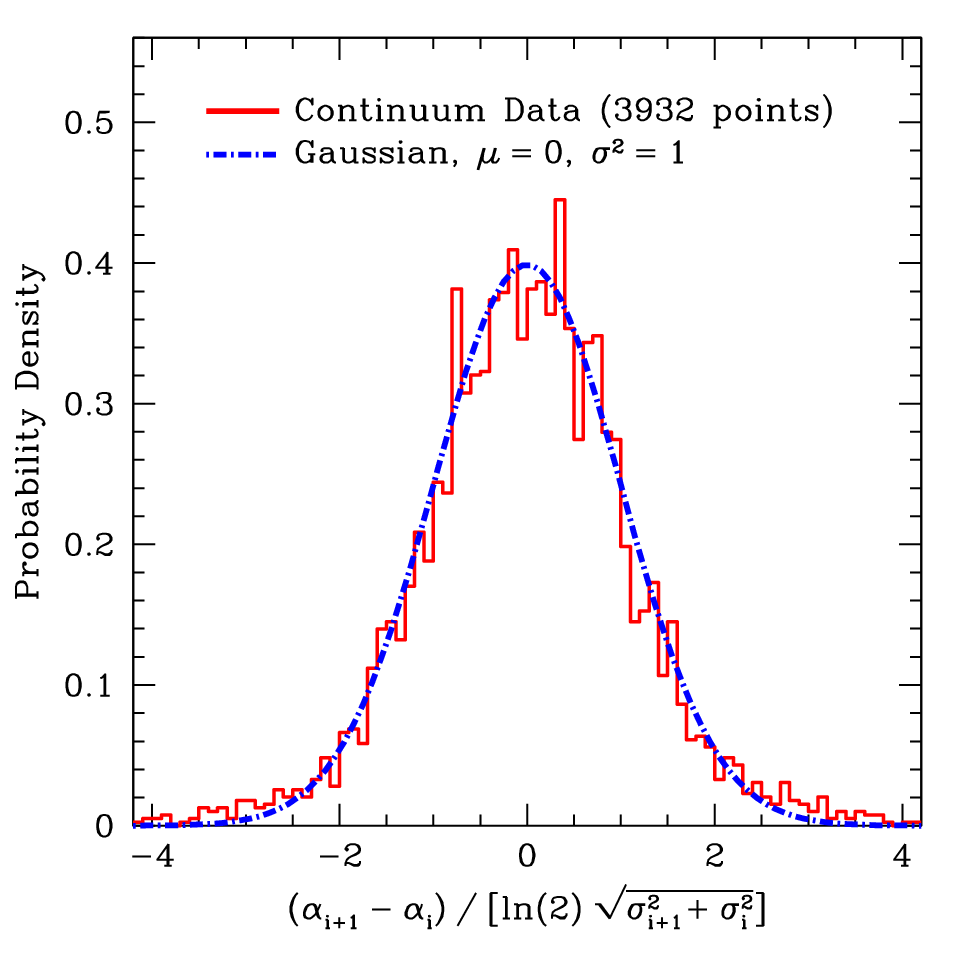
Figure 7 shows that the distribution of as defined by Equation (11) is exceedingly well-fit by a normal distribution with zero mean and unit variance. We have masked 67 of the 3999 normalized intensity differences which lie near the emission lines H, H, [N ii] , [N ii] , [S ii] , and [S ii] . At these wavelengths, real spectral features contribute to the element-to-element variation in . Even with 3932 values of across the wavelength range, a Kolmogorov-Smirnov (K-S) test only detects deviation from Gaussianity with 83% confidence.
The exceptional agreement shown in Figure 7 gives us confidence that our measured errors are reliable and independent (up to a factor of from interpolating). We have verified that coadding neighboring wavelength elements, as we did to smooth the continuum in Section III.1 and to compute the equivalent widths of lines in Section III.2, does not affect the statistical properties of the errors.
IV.2. Biases in the Correlation Spectra
Our model of the correlation between 100 m intensity and optical intensity (Equation (2)) includes errors in the SDSS sky fiber residuals, but neglects (unknown) errors in the 100 m intensity at each fiber’s location and structure unresolved by IRAS. This introduces a wavelength-independent bias to our recovered spectra (Figures 3 - 6). We first derive an expression for the bias and then estimate its value.
The correlation spectrum (Equation (2)) is derived from a minimization. The maximum likelihood values of the and their variances are given by Equations (5) and (6), with and defined in Equations (3) and (4); is the excess 100 m intensity in fiber relative to the average on plate , is the residual sky fiber intensity at wavelength in fiber on plate , and is its variance as estimated by the SDSS pipeline. We let denote the true excess 100 m emission at sky fiber on plate , so that the measurement error, including the effects of unresolved structure, is .
Assuming the model in Equation (2) to be correct, we may write as , with representing the measurement error in the sky fiber intensity. We further assume the error terms and to be uncorrelated with zero mean and invoke the large number of sky fibers (nearly ) to neglect sums of and . The first factor in Equation (5) becomes
| (12) |
This is the same value we would measure with . Noting that the mean 100 m excess, , is zero by construction, our estimate of is biased low by a factor
| (13) |
where is the observed variance in and would be its value with no measurement errors. Thus,
| (14) |
Note that this bias is independent of wavelength and of the errors in the sky fiber intensities. We have empirically verified the latter by adding noise to the intensities; we recover the same correlation spectra to within the errors.
IV.3. Calibrating the Correlation Spectra
An unbiased estimator for , for example a likelihood function of the form
| (15) |
would remove all calibration issues. The SDSS pipeline provides an estimate of , the likelihood of measuring sky fiber residual in sky fiber given a correlation spectrum and true 100 m intensity . Unfortunately, we have almost no information on the errors in the 100 m intensity to estimate , the likelihood of measuring excess 100 m intensity given a true value , and can only guess at a prior, , from the 100 m map itself.
Because of these difficulties, we use two alternative and independent approaches. We first construct an estimator that we expect to be asymptotically unbiased, assuming the error in residual 100 m intensity to depend weakly on the true residual value at a fiber position. This is a reasonable assumption, particularly because we are subtracting the mean 100 m emission over a plate; an -value of zero does not correspond to zero intensity. We then show the results of our radiative transfer calculations assuming ZDA04 dust and a plane-parallel galaxy.
Under the assumption of uniform errors in the residual 100 m intensity, Equation (14) shows that restricting the sample to fibers with large (and therefore large ) will give an asymptotically unbiased estimate. We therefore recalculate between 6600 and 6700 Å using only the fibers with . Figure 8 shows as a function of , calculated by varying from 0 to 4 MJy sr-1; as expected, increases with . Figure 8 suggests a bias factor of at least 1.72. This is also supported by our radiative transfer model, discussed in detail in Section V.1, which suggests a bias of 1.72.4. We conservatively adopt a bias factor of , indicated by the shaded region of Figure 8, to calibrate our correlation spectrum.

V. Discussion
V.1. Scattered Light and Dust Models
Many features of the DGL – the 4000 Å break, broad Mg Fe b absorption, and a much bluer continuum than that of stars with these spectral features – support the hypothesis that the DGL is dominated by scattered starlight. This is hardly surprising, as the spectrum was derived by correlating residual optical intensity with 100 m intensity over small spatial scales. A simplified radiative transfer calculation confirms that our spectrum is consistent with dust scattering and allows us to use the DGL to discriminate between dust models.
Our model of the DGL uses an infinite plane-parallel galaxy with a Gaussian vertical distribution of dust,
| (16) |
with pc [33, 39]. We approximate the stellar distribution as the sum of two exponential distributions with scale heights of 300 pc and 1350 pc [6, 23]. The 300 pc component dominates the distribution with about 90% of the stars.
We use two estimates of the stellar emission spectrum:
- 1.
A model that reproduces the local ISRF of [35], hereafter MMP83, in the midplane, and
- 2.
A stellar population synthesis model from BC03, with solar metallicity and an exponential star formation history over 12 Gyr.
The MMP83 ISRF for Å is approximated as a sum of three dilute blackbodies of , 4000, and 7000 K, with dilution coefficients , , and , respectively. We compute the attenuation of the stellar emission using Equation (A3), setting the attenuated spectrum equal to the local ISRF. In this way, we “de-redden” the MMP83 ISRF to obtain the stellar source spectrum.
We show all of the ISRF spectra in Figure 9. The peak of the de-reddened MMP83 is at about 8000 Å, corresponding to a temperature of 4600 K. The spectrum is similar to a BC03 model with a 5 Gyr star formation timescale, though MMP83 has less UV emission. This is probably a result of the relative lack of early O stars in the Solar neighborhood and of our model’s neglect of extinction from dust in a young star’s birth cloud [9]. The UV discrepancy becomes much more serious for BC03 models with more extended star formation histories. This UV excess significantly increases the dust heating and decreases the ratio of scattering in the optical to emission in the far-infrared. For a star formation timescale of 5 Gyr, this is a 30-40% effect relative to the de-reddened MMP83 model (see Figures 8 and 10).
Theoretical and observational estimates of the local star formation history favor roughly constant star formation rates over 10 Gyr [26, 10]. Such models do not agree with our measured spectrum of the DGL and, using our radiative transfer model, would produce a very different ISRF from MMP83. This may indicate that a substantial fraction of the illuminating starlight originates relatively far from the Solar neighborhood, it may be a result of our simplified radiative transfer, or it may indicate that stars in the Solar neighborhood are generally older than is currently thought. The spatial variation of the DGL (Figure 4) shows that the geometry of the radiative transfer problem is likely to be important. A more detailed model of the Galaxy could better constrain the average stellar source spectrum.

Our radiative transfer calculations neglect multiple scatterings. This is a good approximation at high Galactic latitude where the optical depths are low. It becomes poor near the midplane, but SDSS has very little sky coverage near the Galactic plane (Figure 2). We assume all absorbed starlight to be reradiated isotropically in the infrared and use a Henyey-Greenstein phase function for scattering in the optical. We use the dust model of [15] to convert total infrared power to IRAS 100 m bandpass power, with
| (17) |
The central value corresponds to their model with an incident starlight intensity 80% of that in the Solar neighborhood, which [15] found to provide the best fit to the average far-infrared spectrum measured by [20]. The confidence interval in Equation (17) includes models from 0.5 to 1.5 times the local starlight intensity. Once a dust model is specified, with wavelength-dependent cross-sections, albedos, and anisotropy parameters, our model for the scattered light spectrum has no free parameters. We derive the relevant equations in the Appendix and evaluate them numerically.
Figure 10 shows the results of our calculations to be remarkably insensitive to the details of the galaxy modeling (other than the assumed stellar source spectrum). Though not shown, models with a single exponential distribution of stars and with an exponential, rather than Gaussian, dust distribution, are nearly indistinguishable from the present models. For () the H i has [12] falling below this relation for . For and , we would then expect for , and lower values at . We use for our fiducial distribution.
Figure 11 shows that the optical depths at the SDSS sky fibers, computed using the SFD estimates of and assuming dust, are roughly bracketed by and . This suggests that the sky fiber locations were slightly biased toward lower-than-average H i column densities.


While the details of the model galaxy have little effect on the predicted spectrum, the dust model matters a great deal. The WD01 model appears to have too many large grains, giving too much scattering at long wavelengths. The size distribution of ZDA04 brings our model into much better agreement with the data (see Figure 3). While our model predicts the scattering spectrum to be a very weak function of Galactic latitude, variations in the dust properties, geometry, or illuminating starlight could result in much larger differences. Possible spatial variations in 100 m errors and small-scale structure (Section IV.2) further complicate the interpretation of the spatial variations seen in Figure 4.
V.2. Line Emission
On the evidence presented above, we can be confident that the continuum of the correlation spectrum consists primarily of scattered starlight. It is more difficult to show that the line emission is scattered rather than from ionized gas physically associated with the dust. The strongest piece of evidence is that the equivalent width of H in the correlation spectrum, Å, matches its measured value of 11 Å in the local ISRF (Section III.2). Because scattering will preserve the equivalent width of H in the ISRF incident on the dust, a stronger H line would have indicated an additional, nearly continuum-free component seen in direct emission and correlating with 100 m intensity.
If the emission lines observed in Section III.2 are observed mostly or entirely in reflection, they provide a probe of the average physics of the nearby ISM. As discussed in Section III.2, the strength of the [N ii] and [S ii] lines, combined with the weakness of the [O iii] lines, indicate relatively few photons with eV. This is probably due to the lack of early-type O stars in the Solar neighborhood.

The observed strengths of the collisionally-excited lines relative to recombination lines of similar wavelength are:
| (18) | ||||
| (19) | ||||
| (20) |
These allow us to estimate the temperature of the ISM where the lines originate and the state of ionization of S, N, and O. Figure 12 shows predicted line ratios as functions of electron temperature , calculated using H and H emissivities from Draine [14], collision strengths for N ii from Hudson & Bell [27], for S ii from Tayal & Zatsarinny [48], and for O iii from Aggarwal & Keenan [4]. A density was assumed; the results are insensitive to provided .
Nitrogen is not depleted in the ISM, and the first and second ionization potentials (14.0 and 29.6 eV) lead us to expect N ii/H ii to be close to the solar abundance (N/H) [5]. If we assume (N ii/H ii)/(N/H) we see from Figure 12 that the observed [N ii](6550+6565)/H ratio allows only temperatures K.
Sulfur is not expected to be depleted in H ii regions or the diffuse ISM. With an ionization potential of 23.38 eV for S iiS iii, S ii will be the dominant ionization stage in H ii regions where He is neutral. If we assume S ii/H ii to be between 0.7 and 1.0 the solar abundance (S/H) [5], then we see from Figure 12 that the observed [S ii(6718+6733)]/H requires K.
Oxygen is only slightly depleted in the diffuse ISM, with 20% of the O resident in silicates. The second ionization potential of oxygen is 35.1 eV, and therefore O iii will be present only when He is ionized. A star of spectral type O8 or earlier is required for the He ionization zone to account for more than 50% of the mass in the H ii region [14]. As seen in Table 2, the nearest such stars are 15 Mon (O7V, pc) and Pup (O4I, pc). The reflected light in the DGL is expected to originate mainly within a few hundred pc of the Sun, and therefore the contribution from H ii regions should be dominated by H ii regions where He is neutral and O is singly ionized. Figure 12 shows that the observed strength of [O iii](4960+5008)/H is consistent with O iii/H ii between 0.039 and 0.15 of (O/H) [5]. The observed [O iii] emission can be reproduced by emission from H ii regions with K and O iii/H ii .
He i 5877 is not detected, with a 3- upper limit He i 5877/H; for K, this corresponds to He ii/H ii , which is not a useful constraint.
The emission lines measured in the correlation spectrum are therefore consistent with the line ratios expected for H ii regions within 400 pc of the Sun, for electron temperature K. These temperatures and ionization states are also consistent with the WIM [30], which we expect to contribute a significant fraction of the line emission, particularly at high latitudes.
V.3. The Fraction of Scattered H at High Latitude
The previous section argued that the H in our correlation spectrum is scattered. We can then use the calibrated correlation spectra to estimate the fraction of the observed H at high Galactic latitude that is scattered light. We simply integrate the correlation spectrum over the H line and multiply by the ratio of the total 100 m to H emission over the high latitude sky fibers.
From Figures 8 and 10, we take the ratio m to be . This continuum value allows us to convert an H equivalent width in our correlation spectrum into an intensity relative to the 100 m intensity. We then have
| (21) |
where the H intensity is in Rayleighs11 1 photons cm-2 s-1 sr-1 and we recall (Table 1) that in our correlation spectrum. Our result (21) is close to the value found recently by Witt et al. [50].
Averaging the 100 m intensity from SFD and the H intensity from [19] over all regions with gives a ratio
| (22) |
The ratio of the coefficients in (21,22) gives a scattered fraction of H at high latitudes of . We add the statistical error of 5% in the H equivalent width and our conservative estimate of the uncertainty in the calibration shown in Figure 8 in quadrature, giving a scattered H fraction at high latitude of
| (23) |
Witt et al. [50] produced a scatter diagram of the scattered H fraction (their Fig. 6). The centroid of their distribution appears to be close to our measured value .
Wood & Reynolds [54] estimated that 5–20% of the H at high latitudes would be scattered light from H ii regions. In a theoretical study of the emission spectrum of the diffuse H, Dong & Draine [13] concluded that the observed line ratios, including the low ratio of radio free-free to H, could be understood if 20% of the diffuse H is actually reflected from dust, rather than emission from recombining gas in that direction. All of these results are consistent with our value .
We expect the scattered H to originate both from H ii regions around young stars and from the WIM. Our line ratios seem to be more consistent with those of the WIM than with classical H ii regions [30], which may indicate that the WIM dominates the line emission in our correlation spectra. However, this could also be due to the lack of nearby H ii regions illuminated by early O stars. Our line ratios do seem to be compatible with those in the Per H ii region, which is illuminated by a B0.5sdO system [30, Fig. 12 of].
V.4. Dust Luminescence
We find no evidence of the Extended Red Emission (ERE) observed in some reflection nebulae (e.g., NGC 7023) as a broad emission excess peaking near 7000Å, with a FWHM 1500Å [52, and references therein]; a similar broad excess is reported to be present in the diffuse ISM [24, 47, 51]. The spectrum of light reflected by cirrus clouds was measured by Szomoru & Guhathakurta [47], who reported a broad peak in near 6500Å that was attributed to luminescence, on the grounds that scattering is insufficient. Our study also finds peaking near 6500Å (see Figure 3) but the observed spectrum appears to be consistent with what is expected for scattering. Indeed, our scattering models tend to over-predict the DGL around 70009000 Å (Figure 3), depending on the adopted dust size distribution.
If we posit that the slight excess emission between 5500 Å and 7500 Å over our prediction with the ZDA04 dust model (see Fig. 3) is an upper limit on the ERE, we infer that dust luminescence accounts for no more than 10% of the DGL in this wavelength range and less elsewhere. After calibrating the spectra and relating to the total IR power using Eq. (17), this implies a ratio of ERE to infrared power of 0.4%, or a ratio of ERE to scattered power of 1%.
The ERE will be a function of the intensity of illuminating UV light and the dust column density. It is possible that our technique, which requires spatial variations of the ERE correlated with 100 m intensity over a 1∘ scale, is ill-suited to its detection. If the UV ISRF is particularly weak or spatially variable on small scales, it could at least partially explain the lack of ERE in our correlation spectrum. We have therefore performed two tests.
First, we made our optical depth cutoff more stringent to restrict the calculation to regions optically thin to UV photons. Reducing this cutoff by a factor of 2 had a negligible effect on the correlation spectrum. Unfortunately, when we reduced it further, the main stellar spectral features disappeared and new features similar to those in the high latitude spectrum of Figure 4 appeared. At such low levels of 100 m emission, we expect extragalactic contamination to be significant.
We have also tried to estimate empirically how much of the small-scale variation (over 1∘) in 100 m emission is due to variations in the illuminating starlight and how much is due to variations in the dust column density. We recalculated the correlation spectrum, correlating the SDSS intensities against dust optical depth rather than 100 m intensity. Our recovered correlation spectrum was nearly identical. Unfortunately, the resolution of the SFD temperature map used to convert from 100 m intensity to optical depth, , is too coarse to make this test conclusive.
While we find no evidence of hidden ERE in our correlation spectrum, a more thorough investigation may require instruments that can more directly probe the dust-scattered optical spectrum.
VI. Summary and Conclusions
In this paper, we have measured the spectrum of the scattered component of the DGL using 90,000 calibration spectra from SDSS by correlating against 100 m intensity measured by COBE and IRAS and reduced by SFD. The correlation spectrum of the DGL is consistent with scattering of photons emitted by stars and by ionized gas. Its continuum and lines show interesting variations across the sky, which could be due to differences in the illuminating starlight, in the dust properties, or structure in the Galaxy. Our spectrum is not calibrated because the correlation neglects (unknown) errors and small-scale structure in the 100 m intensity. However, an asymptotically unbiased estimator agrees well with simplified radiative transfer calculations and allows us to calibrate the average spectrum of the DGL. In calibrating the data, we also provide an estimate of the errors and small-scale structure in the SFD 100 m map.
With a simplified radiative transfer calculation assuming a plane-parallel galaxy, we show that the spectrum of the DGL can discriminate between dust models. The ZDA04 dust model is preferred to the WD01 model, which has more large grains and scatters too much red light. The ZDA04 model fits the data very well without requiring dust luminescence as a source of ERE. Indeed, our radiative transfer calculations tend to over-predict scattering redward of 7000 Å.
Our measurement of H in the DGL allows us to indirectly measure the fraction of scattered H at high Galactic latitude. We find an average value of , consistent with the results of Wood & Reynolds [54], Witt et al. [50] and the value inferred by [13]. The line emission also allows us to constrain the properties of local H ii regions. The lack of emission from species with high ionization energies is consistent with the lack of nearby early O stars, and the average scattered spectrum is consistent with gas at 7500 K.
Our results are the product of the extraordinary SDSS, the only dataset of its kind. It would be possible, though difficult, to incorporate the new Baryon Oscillations Spectroscopic Survey spectra [16, BOSS,] into the analysis. The new fibers are smaller (2′′ instead of 3′′), losing far more light and making spectrophotometric calibration much more difficult. The DGL is a sufficiently weak signal that it requires thousands of blank sky spectra to extract useful results. These spectra also need to be in regions with significant dust columns, regions that tend to be avoided by large extragalactic surveys. The SDSS spectra will likely remain the best tool for analyzing the DGL for some time.
While the optical data are unlikely to improve in the near future, WISE and AKARI may allow significant improvements to the infrared map. Our results indicate that the measurement errors and small-scale structure in the SFD 100 m map are nearly as large as the 1∘ variations to which our correlations are sensitive. By combining high resolution infrared data with the SFD maps, we could improve the quality of our DGL spectra and resulting constraints on Galactic stars and dust.
http://www.sdss.org/ .
Appendix A Scattering and Absorption in a Plane-Parallel Exponential Galaxy
We test dust models by calculating scattered spectra in an infinite plane-parallel galaxy, using vertical distributions of stars and dust appropriate to the Solar neighborhood. The Sun is assumed to lie in the midplane, . We calculate the absorption (and hence, infrared emission) and scattering along each line-of-sight, neglecting multiple scatterings.
We denote the (wavelength-dependent) optical depth of dust above height along a vertical line-of-sight as ,
| (A1) |
where is the extinction cross-section and is the dust density. Consider a sheet of stars with uniform surface power density at height . The optical depth from an annulus of stars at a distance from the grain’s projected position in the stellar sheet to a grain at height is
| (A2) |
The total flux density (neglecting multiply scattered photons) incident on a grain at height is then
| (A3) |
where is the exponential integral and is related to by Equation (A1). The total reradiated intensity is an integral of the absorbed fraction of Equation (A3) over all wavelengths and stellar sheets. Defining as the albedo, the total infrared intensity from a sightline at Galactic latitude is
| (A4) |
A dust model, like the [15] model used in Equation (17), is needed to convert into a specific intensity at infrared frequency .
Anisotropic scattering makes it more difficult to calculate the optical intensity. Consider an annulus of the stellar sheet centered directly below a dust grain, and let sweep out the annulus, with pointed away from us. If the dust grain is along a sightline at Galactic latitude , the law of cosines gives the required scattering angle as
| (A5) |
The intensity of light scattered in our direction from a stellar sheet at height is then given by
| (A6) |
with being the normalized phase function and defined by Equation (A2). We use a Henyey-Greenstein phase function for simplicity. If is constant, the integral is trivial and we recover Equation (A3) modulo a factor of . Scattered light is further attenuated by dust along the line-of-sight. Neglecting multiple scatterings, we finally have
| (A7) |
where and are related by Equation (A1) and is defined by Equation (A2). As for Equation (A4), we integrate Equation (A7) over . We do not integrate over wavelength; the spectrum of is shown in Figure 3 normalized by the infrared intensity at 100 m, which is related to by Equation (17). The ratio depends very weakly on Galactic latitude , the normalization of the optical depth, and the details of the stellar and dust distributions. Once an ISRF and dust model are supplied, there are no other free parameters.
References
- [1] Abazajian, K. N., Adelman-McCarthy, J. K., Agüeros, M. A., et al. 2009, ApJS, 182, 543
- [2] Adelman-McCarthy, J. K., Agüeros, M. A., Allam, S. S., et al. 2008, ApJS, 175, 297
- [3] Adelman-McCarthy, J. K., Agüeros, M. A., Allam, S. S., et al. 2006, ApJS, 162, 38
- [4] Aggarwal, K. M., & Keenan, F. P. 1999, ApJS, 123, 311
- [5] Asplund, M., Grevesse, N., Sauval, A. J., & Scott, P. 2009, ARA&A, 47, 481
- [6] Binney, J., & Merrifield, M. 1998, Galactic Astronomy (Princeton, NJ: Princeton University Press)
- [7] Boggess, N. W., Mather, J. C., Weiss, R., et al. 1992, ApJ, 397, 420
- [8] Bruzual, G., & Charlot, S. 2003, MNRAS, 344, 1000
- [9] Charlot, S., & Fall, S. M. 2000, ApJ, 539, 718
- [10] Cignoni, M., Degl’Innocenti, S., Prada Moroni, P. G., & Shore, S. N. 2006, A&A, 459, 783
- [11] Dennison, B., Simonetti, J. H., & Topasna, G. A. 1998, PASA, 15, 147
- [12] Dickey, J. M., Terzian, Y., & Salpeter, E. E. 1978, ApJS, 36, 77
- [13] Dong, R., & Draine, B. T. 2011, ApJ, 727, 35
- [14] Draine, B. T. 2011, Physics of the Interstellar and Intergalactic Medium (Princeton, NJ: Princeton University Press)
- [15] Draine, B. T., & Li, A. 2007, ApJ, 657, 810
- [16] Eisenstein, D. J., Weinberg, D. H., Agol, E., et al. 2011, AJ, 142, 72
- [17] Elsässer, H., & Haug, U. 1960, ZAp, 50, 121
- [18] Elvey, C. T., & Roach, F. E. 1937, ApJ, 85, 213
- [19] Finkbeiner, D. P. 2003, ApJS, 146, 407
- [20] Finkbeiner, D. P., Davis, M., & Schlegel, D. J. 1999, ApJ, 524, 867
- [21] Frieman, J. A., Bassett, B., Becker, A., et al. 2008, AJ, 135, 338
- [22] Gaustad, J. E., McCullough, P. R., Rosing, W., & Van Buren, D. 2001, PASP, 113, 1326
- [23] Gilmore, G., & Reid, N. 1983, MNRAS, 202, 1025
- [24] Gordon, K. D., Witt, A. N., & Friedmann, B. C. 1998, ApJ, 498, 522
- [25] Henry, R. C. 1981, ApJ, 244, L69
- [26] Hernández, X., Avila-Reese, V., & Firmani, C. 2001, MNRAS, 327, 329
- [27] Hudson, C. E., & Bell, K. L. 2005, A&A, 430, 725
- [28] Hurwitz, M., Bowyer, S., & Martin, C. 1991, ApJ, 372, 167
- [29] Lillie, C. F., & Witt, A. N. 1976, ApJ, 208, 64
- [30] Madsen, G. J., Reynolds, R. J., & Haffner, L. M. 2006, ApJ, 652, 401
- [31] Maíz Apellániz, J., Alfaro, E. J., & Sota, A. 2008, ArXiv e-prints, 0804.2553
- [32] Maíz-Apellániz, J., Walborn, N. R., Galué, H. Á., & Wei, L. H. 2004, ApJS, 151, 103
- [33] Malhotra, S. 1995, ApJ, 448, 138
- [34] Martin, C., Hurwitz, M., & Bowyer, S. 1990, ApJ, 354, 220
- [35] Mathis, J. S., Mezger, P. G., & Panagia, N. 1983, A&A, 128, 212
- [36] Morgan, D. H., Nandy, K., & Thompson, G. L. 1978, MNRAS, 185, 371
- [37] Murthy, J., Henry, R. C., Feldman, P. D., & Tennyson, P. D. 1990, A&A, 231, 187
- [38] Murthy, J., Henry, R. C., & Holberg, J. B. 1991, ApJ, 383, 198
- [39] Nakanishi, H., & Sofue, Y. 2003, PASJ, 55, 191
- [40] Neugebauer, G., Habing, H. J., van Duinen, R., et al. 1984, ApJ, 278, L1
- [41] Planck Collaboration, Ade, P. A. R., Aghanim, N., et al. 2011, ArXiv e-prints, 1101.2029
- [42] Reynolds, R. J., Haffner, L. M., & Madsen, G. J. 2002, in ASPC, Vol. 282, Galaxies: the Third Dimension, ed. M. Rosada, L. Binette, & L. Arias, 31
- [43] Sasseen, T. P., & Deharveng, J.-M. 1996, ApJ, 469, 691
- [44] Schlegel, D. J., Finkbeiner, D. P., & Davis, M. 1998, ApJ, 500, 525
- [45] Seon, K.-I., Edelstein, J., Korpela, E., et al. 2011, ApJS, 196, 15
- [46] Stoughton, C., Lupton, R. H., Bernardi, M., et al. 2002, AJ, 123, 485
- [47] Szomoru, A., & Guhathakurta, P. 1998, ApJ, 494, L93
- [48] Tayal, S. S., & Zatsarinny, O. 2010, ApJS, 188, 32
- [49] Weingartner, J. C., & Draine, B. T. 2001, ApJ, 548, 296
- [50] Witt, A. N., Gold, B., Barnes, F. S., III, et al. 2010, ApJ, 724, 1551
- [51] Witt, A. N., Mandel, S., Sell, P. H., Dixon, T., & Vijh, U. P. 2008, ApJ, 679, 497
- [52] Witt, A. N., & Vijh, U. P. 2004, in ASPC 309, Astrophysics of Dust, ed. A. N. Witt, G. C. Clayton, & B. T. Draine (San Francisco, CA: ASP), 115
- [53] Wolstencroft, R. D., & Rose, L. J. 1966, Nature, 209, 388
- [54] Wood, K., & Reynolds, R. J. 1999, ApJ, 525, 799
- [55] Yahata, K., Yonehara, A., Suto, Y., et al. 2007, PASJ, 59, 205
- [56] York, D. G., Adelman, J., Anderson, J. E., Jr., et al. 2000, AJ, 120, 1579
- [57] Zubko, V., Dwek, E., & Arendt, R. G. 2004, ApJS, 152, 211
- [58] Zvereva, A. M., Severnyi, A. B., Granitskii, L. V., et al. 1982, A&A, 116, 312