Pricing Weather Derivatives for Extreme Events

We begin by introducing the model used for modeling maxima (minima can always be rewritten as $\min(Y_{1},...,Y_{n})=-\max(-Y_{1},...,-Y_{n})$, so there is no loss in generality when one considers only maxima). Let $Y_{1},...,Y_{n}$ be independent and identically distributed univariate random variables with some distribution function $F$, and let $M_{n}=\max(Y_{1},...,Y_{n})$ be the maximum. If $M_{n}$ converges to a non-degenerate distribution under re-normalization as

for some sequences $a_{n}$ and $b_{n}$, then $G$ must be a member of the Generalized Extreme Value (GEV) family, with distribution function

Here $a_{+}=\mbox{max}(a,0),$ and $\mu,\sigma,$ and $\xi$ are the location, scale, and shape parameters, respectively (Coles, 2001). The sign of the shape parameter $\xi$ corresponds to the three classical extreme value distributions: $\xi>0$ is Fréchet, $\xi<0$ is Weibull, and $\xi\rightarrow 0$ (in the limit) is Gumbel. The Fréchet case corresponds to a heavy tailed distribution, Gumbel is intermediate, and Weibull has a bounded upper limit.

In practice, it isn’t necessary to worry about specifying sequences $b_{n}$ and $a_{n}$ due to the property of max-stability: If $Y_{1},...,Y_{n}$ are independent and identically distributed from $G$, then $\max(Y_{1},...,Y_{n})$ also has the same distribution with only a change in location and scale, as $G^{n}(y)=G(A_{n}y+B_{n})$ for constants $A_{n}$ and $B_{n}$. A distribution is a member of the Generalized Extreme Value family if and only if it is max-stable (Leadbetter et. al., 1983). A practical consequence of this property is that if one changes the block size (from monthly maxima to annual maxima, for instance) and fits a new model, new estimates for the three GEV parameters ($\mu,\sigma,\xi)$ are obtained, but the model is still GEV.

A special case of the Generalized Extreme Value family is the unit-Fréchet, with distribution function $G(m)=\exp(-{1}/{m})$. Any member of the Generalized Extreme Value family may be transformed to have unit-Fréchet margins as follows: if $Y$ has a Generalized Extreme Value distribution with range $0<Y<\infty$, then a new variable $U$ may be defined as

and $U$ has unit-Fréchet margins. If the parameters are unknown, they may first be estimated and then the transformation to $U$ is taken. When we model multivariate or spatial extremes, there is no loss in generality when one assumes the margins are all unit-Fréchet. In practice, one would first estimate all marginal distributions and transform to unit-Fréchet, then in a second step analyze the spatial dependence.

The GEV model can be fit to observed data using maximum likelihood estimation. Call the parameter vector $\phi$. This parameter can be as simple as three fixed parameters, as $\phi=(\mu,\sigma,\xi)$. Alternatively, one can model the GEV parameters using temporal or spatial covariates. A few examples include $\mu=\mu_{1}+\mu_{2}\cdot t$, where $t$ is time, or $\sigma=\sigma_{1}+\sigma_{2}\cdot lat+\sigma_{3}\cdot lon+\sigma_{4}\cdot elev$, which considers effects of latitude, longitude, and elevation on the scale parameter. No matter the structure of the parameter $\phi$, define the density function $g(m;\phi)=\frac{d}{dm}G(m;\phi)$. Then, the maximum likelihood estimate of $\phi$ is

This maximization is often done numerically, and has been implemented in a number of software programs including R (R Development Core Team, 2010) using the function fgev in the package evd. The density function for the fitted model is obtained by plugging in the maximum likelihood estimate as $g(m;\hat{\phi}_{MLE}).$

Once we have a fitted model, we can use this to estimate the necessary pure premium and risk loading. This requires estimates of the first two moments of the unknown payment variable $L$, as

where $L(m;s,t)^{d}$ is the loss payment for realization $M=m$ raised to the $d^{th}$ power ($d=1$ or $2$), and $g(m)$ is the density function of the maxima. The first type of weather derivative discussed has $L(m;s,t)^{d}=\alpha^{d}$ for $m\geq s$, which means the integral can be evaluated exactly as

The second and third types of derivatives involve more complicated integrals, so we use monte carlo techniques to estimate them. This approach can be used to estimate moments for other types of derivatives with even more complicated payment structures, and is thus the most general approach. Here we draw a large iid sample $M_{i}\sim G(m)$ for $i=1,...,I$, and for each draw we compute the payment $L(m_{i})$. Assuming that $E(|L(M)|^{2})$ is finite, then by the Strong Law of Large Numbers as $I\rightarrow\infty$, sample means converge to the first and second moments as (Robert, 2007)

and

Furthermore, if the fourth moment is finite, as $\int L(m)^{4}g(m)\,dm<\infty$, then by the Central Limit Theorem we know that the sample average in equation 6 is asymptotically normal with variance $\mbox{var}(L(M))/I$, and the sample average in equation 7 is asymptotically normal with variance $\mbox{var}(L(M)^{2})/I$. We estimate the expected payments under the second and third contracts by drawing $M_{1},...,M_{I}\sim G(m\mid\hat{\phi})$, and compute $L(m_{i})$ and $L(m_{i})^{2}$ for each of draw using $I=1,000,000$ total draws. This total number was chosen to provide highly accurate estimates within a reasonable time, and simulations showed it was sufficiently high to eliminate concern for purely numerical monte carlo error. Sample averages of each converge to the theoretical first and second moments, which are used in the pricing model. One example of a risk-loaded premium based on marginal variance is

for some dollar amount $\lambda$, chosen to satisfy some risk tolerance criteria.

As an example of how this model may be used, consider pricing a weather derivative with payments whenever the maximum daily summer temperature in the city of Phoenix, AZ exceeds some high threshold $s$. On June 26, 1990, Phoenix airport was forced to close because the temperature exceeded 122 degrees Fahrenheit. Aircraft operating manuals did not provide information for takeoff and landing procedures in temperatures above 120 degrees Fahrenheit. The closure caused the predictable sort of economic disruption which accompanies airport closures. We envision a weather derivative as a useful tool in this situation.

To price the derivative, we collect maximum daily summer temperatures at the Phoenix airport, $y_{i,j}$ for year $i$ and day $j$, where $j=1,...,92$ (the 92 days in June, July, and August) for years 1933 to 2010. This data comes from the National Climate Data Center. For each year $i$, we take the block maximum $m_{i}=\max(y_{i,1},...,y_{i,92})$, and model these annual maxima $m_{i}$ as a Generalized Extreme Value distribution. Plotting these data, we observe evidence of a slight positive trend over time (figure 1). A simple linear model of maximum temperature versus year shows a statistically significant positive slope of 0.03363, with p-value 0.007. We also find no evidence that annual maximum temperatures are autocorrelated.

We estimate the GEV parameter $\phi$ using maximum likelihood estimation, as shown in equation 4, but with the possibility of a trend on the location parameter, as $\mu=\mu_{1}+\mu_{2}\cdot t$ where $t$ is year. Thus, the GEV parameter here is actually $\phi=(\mu_{1},\mu_{2},\sigma,\xi)$. The maximum likelihood estimates (with standard errors shown in brackets) are $\hat{\mu}_{1}=113.367\hskip 5.69054pt[0.250]$, $\hat{\mu}_{2}=0.035\hskip 5.69054pt[0.011]$, $\hat{\sigma}=1.931\hskip 5.69054pt[0.176]$, and $\hat{\xi}=-0.090\hskip 5.69054pt[0.078]$. Figure 2 shows some common diagnostics and the return level plot. The return level plot shows the expected number of years before an exceedance of a certain level is reached. This is the same as the reciprocal of the probability of a specified exceedance, and forms the basis for statements such as describing an event as a“once every 50 years" event.

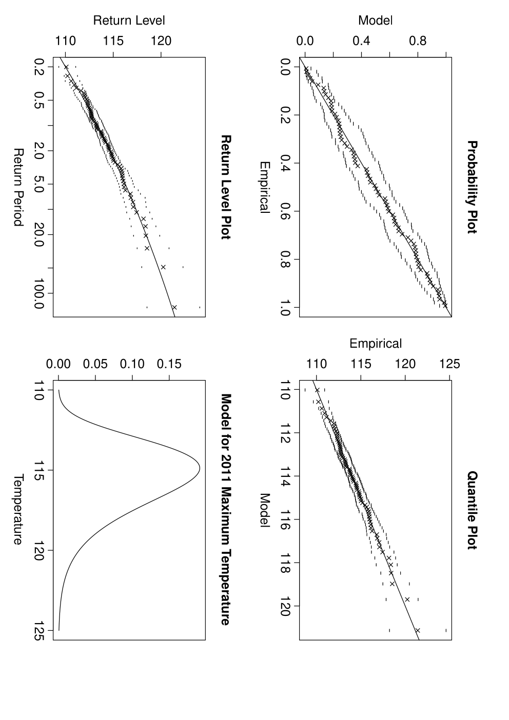
With the fitted model for maximum summer temperature, we can estimate the first and second moments of various weather derivative payments in the year 2011. Estimated moments for the three types of derivatives from section 1 are shown in tables 1, 2, 3, and 4. As the limit $t\rightarrow\infty$, payments under the second and third types are equal.

Tables like these can be used to price a wide range of weather derivatives. Consider a weather derivative with payment $1000\cdot(M-118)$ for $M\leq 125$ and $7000$ for $M\geq 125$, where $M$ is the maximum summer temperature in Phoenix. Using equation 8 with $\lambda=0.0001$, the tables show the pure premium should be $223.89+0.0001\cdot(618.16\cdot 10^{3}-223.89^{2})=280.69$. Premiums for other limits, strike values, and payment structures can be estimated from the same general approach once a fitted model has been obtained.

The basic object in spatial statistics is a stochastic process $Y(x),x\in X$ where $X$ is a subset of $R^{p}$, usually with $p=2$. Let

be the mean of the process defined for all of $X$, and assume that the variance of $Y(x)$ exists everywhere in $X$. The process is said to be Gaussian if for any $K\geq 1$ and locations $x_{1},...,x_{K}$, the vector $(Y(x_{1}),...,Y(x_{K}))$ has a multivariate normal distribution. The process is strictly stationary if the joint distribution of $(Y(x_{1}),...,Y(x_{K}))$ is the same as $(Y(x_{1}+h),...,Y(x_{K}+h))$ for any $h\in X$ and for any $K$ points $x_{1},...,x_{K}$. For a Gaussian process, strict stationarity implies

That is, the covariance of the process at any two locations is some function $C$ which depends only on the separation vector between points, and not the particular locations. This is also called second-order stationarity. Next, we define the variogram through the relation

where the quantity $2\gamma$ is the variogram, and $\gamma$ is the semi-variogram. Under the assumption of strict (or second-order) stationarity,

where $\rho(h)$ is the correlation between two locations separated by vector $h$. Further, if we have $\gamma(h)=\gamma(||h||)$ for all $h\in X$, meaning if the semi-variogram only depends on $h$ through its length $||h||$, then the process is isotropic. The correlation function $\rho(h)$ is then usually chosen from one of the valid families of correlations for Gaussian processes. A few common choices are Whittle-Matérn,

Cauchy,

and powered exponential

where $c_{1},c_{2}$ and $\nu$ are the nugget, range, and smooth parameters, $\Gamma$ is the gamma function and $K_{\nu}$ is the modified Bessel function of the third kind with order $\nu$. It is common to fix the nugget as $c_{1}=1$, which forces $\rho(h)\rightarrow c_{1}=1$ as $h\rightarrow 0$. This is a reasonable assumption for many environmental processes, and we make this assumption throughout this paper and do not attempt to model the nugget. Throughout the remainder of this paper, the unknown spatial dependence parameter is called $\theta=(c_{2},\nu)$.

The final definition we need before we can introduce the model for spatial extremes is the multivariate extreme value distribution. Let $(Y_{i1},...,Y_{iK})$, $i=1,...,n$ be independent and identically distributed replicates of a $K-$dimensional random vector and let $M_{n}=(M_{n1},...,M_{nK})$ be the vector of componentwise maxima, where $M_{nk}=\max(Y_{1k},...,Y_{nk})$ for $k=1,...,K$. A non-degenerate limit for $M_{n}$ exists if there exist sequences $a_{nk}>0$ and $b_{nk}$, $k=1,...,K$ such that

Then $G$ is a multivariate extreme value distribution, and is max-stable in the sense that for any $n\geq 1$ there exist sequences $A_{nk}>0$, $B_{nk}$, $k=1,...,K$ such that

The marginal distributions of a multivariate extreme value distribution are necessarily univariate Generalized Extreme Value distributions.

Here we introduce the spatial analog of the multivariate extreme value distribution. Let $Z(x),x\in X\subseteq R^{p}$ be a stochastic process. If for all $n\geq 1$, there exist sequences $a_{n}(x),b_{n}(x)$ for some $x_{1},...,x_{K}\in X$ such that

then $G_{x_{1},...,x_{K}}$ is a multivariate extreme value distribution. If the above holds for all possible $x_{1},...,x_{K}\in X$ for any $K\geq 1$, then the process is a max-stable process. To briefly summarize, if we have a max-stable process $Z(x)$ defined for all $x\in X$, then at any single location $x\in X$ the distribution of $Z(x)$ is GEV, and all finite vectors $(Z(x_{1}),...,Z(x_{K}))$ follow a multivariate extreme value distribution. In this sense, max-stable processes are the infinite dimensional generalization of multivariate extremes, and nicely extend the GEV to spatial domains.

Constructing a max-stable process is accomplished through a point process approach. Let $Y(x)$ be a non-negative stationary process on $R^{p}$ such that $E(Y(x))=1$ at each $x$. Let $\Pi$ be a Poisson process on $R_{+}$ with intensity $dw/w^{2}$. If $Y_{i}(x)$ are independent replicates of $Y(x)$, then

is a stationary max-stable process with unit Fréchet margins (De Haan, 1984). From this, the joint distribution may be represented as

Varying the choice of the process $Y(x)$ gives different max-stable processes. Smith (unpublished manuscript, 1990) constructed a process known as the Gaussian extreme value process by taking $Y_{i}(x)$ to be a multivariate Gaussian centered at the point $x_{i}$ with covariance matrix $\Sigma$. Smith also introduced the “rainfall-storms" interpretation in 2 dimensions: think of $R^{2}$ as the space of storm centers, $s_{i}$ as the magnitude of the $i^{th}$ storm, and $Y_{i}(x)$ as the shape of the storm centered at position $x_{i}$. The maximum of independent storms at each location $x$ is taken to be the max-stable process. A realization of this process is shown in figure  3. A particular strength of the Smith model is the ability to handle anisotropy, as shown in the figure. This comes from the off diagonal covariance parameter $\Sigma_{12}$ in

We will consider the use of the Smith model only to check the assumption of isotropy, which is required for the next class of max-stable processes. Schlather (2002) introduced a flexible set of models for max-stable processes, termed extremal Gaussian processes. Consider a stationary Gaussian process $Y(x)$ on $R^{p}$ with correlation function $\rho(\cdot;\theta)$ and finite mean $\delta=E\max(0,Y(x))\in(0,\infty)$. Let $w_{i}$ be a Poisson process on $(0,\infty)$ with intensity measure $\delta^{-1}w^{-2}ds$. Then

is a stationary max-stable process with unit-Fréchet margins. The bivariate distribution function is

where $\rho(h;\theta)$ is the correlation of the underlying Gaussian process $Y(x)$ and $h=||x_{1}-x_{2}||$. Figure 3 shows one realization of a process with the Whittle-Matérn correlation function. These processes are flexible, and produce plausible realizations of environmental processes. We have elected to concentrate on the Schlather model in this paper.

A potential stumbling block to using max-stable processes is that the closed-form expression of the joint likelihood shown in equation 9 can only be written out for dimension one or two. This means only the univariate likelihood (which is GEV) and bivariate likelihood function (as shown in equation 10) are available in closed form. When one considers the joint distribution of a max-stable process at three or more locations, a closed-form expression for the joint likelihood is unavailable. One way to proceed with a likelihood-based approach is to substitute the composite likelihood for the unavailable joint likelihood. The composite log-likelihood is defined as

where each term $f(z_{i,n},z_{j,n};\theta)$ is a bivariate marginal density function based on locations $i$ and $j$. The two inner sums sum over all unique pairs, while the outer sums over the $N$ i.i.d. replicates. Similar to the full likelihood function, the parameter which maximizes a composite log likelihood can be found, and is termed a maximum composite likelihood estimate, or MCLE. The maximum composite likelihood estimator is consistent and asymptotically normal (Lindsay, 1988) (Cox and Reid, 2004) as

where $H(\theta)=E(-H_{\theta}\ell_{C}(\theta;Z))$ is the expected information matrix, $J(\theta)=V(D_{\theta}\ell_{C}(\theta;Z))$ is the covariance of the score, and $H_{\theta}$ is the Hessian matrix, $D_{\theta}$ is the gradient vector, and $V$ is the covariance matrix. In the setting with the full likelihood and MLE, we have $H(\theta)=J(\theta)$, but for the composite likelihood setting these matrices are not equal.

Padoan et. al. (2010) used composite likelihoods to model the joint spatial dependence of extremes, and implemented their work in the R package SpatialExtremes. The maximum composite likelihood estimator $\hat{\theta}_{MCLE}$ is found using the numerical optimizer command optim. Estimates of the variances are found by plugging in $\hat{\theta}_{MCLE}$ into expressions for $H$ and $J$:

Model selection is based on minimizing the composite likelihood information criteria (CLIC) (Varin and Vidoni, 2005), equal to

where the second term is the composite log-likelihood penalty term.

In our setting, this approach is used as follows: we begin with $Y$ independent and identically distributed realizations of an observed set of spatial extremes data, for locations $x_{1},...,x_{K}$. Thus there are $Y$ replicates and $K$ locations. For each location $x_{k}$, we transform the GEV data to unit-Fréchet margins by first estimating all GEV parameters $\hat{\mu}(x_{k}),\hat{\sigma}(x_{k}),\hat{\xi}(x_{k}),k=1,...,K$, then using these in the transformation shown in equation 3. Next we obtain the maximum composite likelihood estimate for the dependence parameter $\widehat{\theta}_{MCLE}=(\hat{c}_{2},\hat{\nu})$ of the max-stable process using the composite likelihood approach outlined above. The result is a fitted model for the extremes at the $K$ specific locations, with spatial GEV parameter $\hat{\phi}=(\hat{\mu}(x_{k}),\hat{\sigma}(x_{k}),\hat{\xi}(x_{k}),k=1,...,K)$ and spatial dependence parameter $\hat{\theta}=(\hat{c}_{2},\hat{\nu})$.

We evaluate the approach through simulations, first with a single detailed case and then larger numbers of simulations. It will be convenient to define some new notation to keep simulation results clear. Call the true full parameter $\theta=(\mu(x_{1}),\sigma(x_{1}),\xi(x_{1}),...,\mu(x_{K}),\sigma(x_{K}),\xi(x_{K}),c_{2},\nu)$, and the estimated parameter $\hat{\theta}$. Call the true marginal variance $MV(\theta)$, and call an estimate of this based on a fitted model $\widehat{MV}(\hat{\theta})$. We begin with a single detailed case.

We simulated a max-stable process with parameters chosen to mimic annual temperature maxima in North America. The process had unit-Fréchet margins and Whittle-Matérn covariance with dependence parameter $(c_{1},c_{2},\nu)=(1,3,1)$ for 75 years at 20 locations randomly placed on a 10 by 10 grid. Call the vertical dimension latitude ($lat$) and the horizontal longitude ($lon$). To make this data consistent with annual temperature maxima, at each location we transformed to the GEV scale by specifying parameters $\mu(x)=110-lat/2$, $\sigma(x)=1.5+lat/5,$ and $\xi(x)=-0.1$. The basic idea was to imagine higher latitude locations having overall lower extreme temperatures, but higher variability of extremes. We used these transformations for each of the 20 locations to produce a max-stable process with GEV($\mu(x),\sigma(x),\xi(x)$) margins. We fix this as the “observed" data.

Next, we analyzed these data using composite likelihood estimation. For each location $x_{k}$, we obtained a maximum likelihood estimate $\hat{\phi}(x_{k})=\hat{\mu}(x_{k}),\hat{\sigma}(x_{k}),\hat{\xi}(x_{k}),k=1,...,K$ using equation 4, and then used these to transform each margin to unit-Fréchet using equation 3. We fit a max-stable process with Whittle-Matérn correlation with nugget parameter 1, and obtained maximum composite likelihood estimate $(\hat{c}_{2},\hat{\nu})$. Using this fitted model, we simulated a large number of processes and transformed them to the temperature scale using $\hat{\mu}(x_{k}),\hat{\sigma}(x_{k}),\hat{\xi}(x_{k})$ at each location $x_{k}$.

Thus we have described a means of simulating $i=1,...,I$ extreme temperature events $m_{i,k}$ for locations $x_{1},...,x_{K}$ from our fitted model. This information was used to estimate payments for weather derivatives by computing $L(m_{i,k};s,t)$ . Table 5 shows results from one simulation. We simulated 200,000 extreme temperature events at the same 20 locations, and used these to compute payments $L_{i,k}$ for $i=1,...,200,000$ and $k=1,...,K$. Shown are payments for a weather derivative paying 1 when $T\geq 112$, the aggregate payment $\sum_{k=1}^{19}L_{k}$, and the payments for a possible weather derivative $L_{20}$. The marginal variance of adding the $20^{th}$ derivative was estimated as $\widehat{MV}_{20}(\hat{\theta})=22.788-21.216=1.572$, which is clearly much larger than 0.081, the estimated variance of the payments when dependence terms are ignored. An additional 200,000 simulations from the true model with parameter $\theta$ shows the true marginal variance $MV_{20}(\theta)$ is 1.250. This particular simulation showed an overestimation of the marginal variance of 25.7%, which is clearly a substantial error, but not when compared to the error from ignoring spatial dependence.

We evaluated the performance of this method in estimating the marginal variance of adding a $4^{th}$ weather derivative to an existing portfolio composed of $L_{1},L_{2}$, and $L_{3}$. This quantity is key to pricing a risk load for $L_{4}$. We randomly placed $K=25$ locations on a 10 by 10 grid, and randomly selected 4 of these to represent locations of weather derivatives. The target quantity was $MV_{4}$, the marginal variance of adding a fourth derivative. We estimated this quantity using two methods:

1. 1.

   Estimate $MV_{4}$ using equation 18, which accounts for spatial dependence by fitting a max-stable process and uses simulations from the model, with fitted parameter $\widehat{\theta}=(\hat{\mu}(x_{1}),\hat{\sigma}(x_{1}),\hat{\xi}(x_{1}),...,\hat{\mu}(x_{4}),\hat{\sigma}(x_{4}),\hat{\xi}(x_{4}),\hat{c_{2}},\hat{\nu})$.

2. 2.

   Estimate $MV_{4}$ using equation 17, which fits a GEV to the data at location $k=4$ but does not account for spatial dependence among the derivatives, with fitted parameter is $\widehat{\theta}=(\hat{\mu}_{4},\hat{\sigma}_{4},\hat{\xi})$.

Again, call the true full parameter $\theta=(\mu(x_{1}),\sigma(x_{1}),\xi(x_{1}),...,\mu(x_{K}),\sigma(x_{K}),\xi(x_{K}),c_{2},\nu)$, and the estimated parameter $\hat{\theta}$. Call the true marginal variance $MV(\theta)$, and an estimate $\widehat{MV}(\hat{\theta})$. The true marginal variance was found by simulating $I=1,000,000$ realizations of a max-stable process under the true parameter $\theta$, and using equation 18. Method 1 uses the same approach, but with estimated parameter $\hat{\theta}$, as we showed in the single example above. Method 2 ignores spatial dependence. The first measure of error we use is percentage error,

where $j=1,...,500$ refers to a simulation run. This choice preserves the sign of estimation error. Results are shown in figure 4. Here, we see the peril of ignoring spatial dependence of losses in a collection of weather derivatives. The right column shows that as the range of the spatial dependence increases, the underestimation bias of estimating marginal variance $MV_{4}$ increases. The left column shows the unbiased results obtained from incorporating dependence using the method of this paper.

We also show the asymptotic results for Method 1 in table 6. Here, we use a slight variant of estimation error called mean absolute percentage error,

This choice does not preserve the sign of error, but is more suited to showing asymptotic results. Results from 150 simulations in a variety of years and dependence ranges are shown in table 6. For all dependence ranges shown, the error in estimation falls as more data is available. The remaining error is primarily due to parameter estimation error in $\widehat{\theta}$ .

Here we discuss using the models to price a risk load. Feldblum (1990) described five methods for an insurer to determine the risk load for writing a policy with unknown loss $L$. The first two methods discussed were the variance approach, where $R=\lambda\cdot\mbox{var}(L)$, and the standard deviation approach, where $R=\lambda\cdot\sqrt{\mbox{var}(L)}$. Kreps (1990) and also Philbrick (1991) discussed how a new policy adds risk through the marginal increase in total variance, shown in equation 18. Gogol (1992) cautioned that these methods of pricing risk loads are order-dependent if losses are correlated, leading to a mismatch between individual renewal risk loads and the total portfolio risk load, best illustrated by a toy example.

Consider two correlated policies, $L_{1}$ and $L_{2}$, and consider computing the risk load based on marginal variance in two ways:

1. 1.

   A risk load using marginal variance for the total loss $L=L_{1}+L_{2}$ would be
   $\lambda\left(\mbox{var}(L_{1})+\mbox{var}(L_{2})+2\cdot\mbox{cov}(L_{1},L_{2})\right)$.

2. 2.

   A risk load computed individually would go as follows: when $L_{2}$ is priced, the risk load is $\lambda(\mbox{var}(L_{2})+2\cdot\mbox{cov}(L_{1},L_{2}))$. When $L_{1}$ renews, it receives risk load $\lambda(\mbox{var}(L_{1})+2\cdot\mbox{cov}(L_{1},L_{2}))$. The sum of these renewal risk loads is $\lambda\left(\mbox{var}(L_{1})+\mbox{var}(L_{2})+4\cdot\mbox{cov}(L_{1},L_{2})\right)$, which has double counted the covariance terms and does not match the total portfolio risk load.

References

- Coles (2001) Coles, S. (2001). An Introduction to Statistical Modeling of Extreme Values. London, Springer.
- Cox and Reid (2004) Cox, D., Reid, N. (2004). A note on pseudo-likelihood constructed from marginal densities. Biometrika, 91:729-737.
- Cressie (1993) Cressie, N. (1993). Statistics for Spatial Data. New York, Wiley Interscience.
- De Haan (1984) De Haan, L. (1984). A spectral representation for max-stable processes. The Annals of Probability. 12:1194-1204.
- Embrechts, et. al. (1999) Embrechts, P., Resnick, S., Samorodnitsky, G. (1999). Extreme Value Theory as a Risk Management Tool. North American Actuarial Journal 26, pp. 30-41.
- Feldblum (1990) Feldblum, S. (1990). Risk Loads for insurers. Proceedings of the Casualty Actuarial Society LXXVII, 160-195.
- Jewson and Brix (2005) Jewson, S. and Brix, A. (2005). Weather Derivative Valuation. Cambridge University Press, 2005.
- Kreps (1990) Kreps, R. (1990). Reinsurer Risk Loads from Marginal Surplus Requirements. Proceedings of the Casualty Actuarial Society LXXVII, 196-203.
- Kunreauther and Michel-Kerjan (2009) Kunreuther, H., Michel-Kerjan, E. (2009). At War with the Weather: Managing Large-Scale Risks in a New Era of Catastrophes The MIT Press, 2009.
- Gogol (1992) Gogol, D. (1992). Discussion of Kreps: Reinsurer Risk Loads from Marginal Surplus Requirements. Proceedings of the Casualty Actuarial Society LXXIX, 362-366.
- Goodwin and Smith (1995) Goodwin, B., Smith, V. (1995). The Economics of Crop Insurance and Disaster Aid The AEI Press, 1995.
- Leadbetter et. al. (1983) Leadbetter, M., Lindgren, G., Rootzén, H. (1983). Extremes and Related Properties of Random Sequences and Series. New York, Springer Verlag.
- Lindsay (1988) Lindsay, B. (1988). Composite likelihood methods. Contemporary Mathematics, 80:221-239.
- Mango (1998) Mango, D. (1998). An Application of Game Theory: Property Catastrophe Risk Load Proceedings of the Casualty Actuarial Society LXXXV, pp. 157-186.
- Mikosch (2006) Mikosch, T. (2006). Copulas: Tales and Facts. Extremes, 9:3-20.
- Padoan et. al. (2010) Padoan S., Ribatet M., Sisson S. (2010). Likelihood-based inference for max-stable processes. JASA, 105(489):263-277
- Philbrick (1991) Philbrick, S. (1991). Discussion of Feldblum: Risk Loads for Insurers. Proceedings of the Casualty Actuarial Society LXXVIII, 56-63.
- R Development Core Team (2010) R Development Core Team (2010). R: A language and environment for statistical computing. R Foundation for Statistical Computing, Vienna, Austria. ISBN 3-900051-07-0, URL http://www.R-project.org.
- Richards et. al. (2004) Richards, T., Manfredo, M., Sanders, D. (2004). Pricing Weather Derivatives. American Journal of Agricultural Economics, 86(4), 1005-1017.
- Robert (2007) Robert C. (2007). The Bayesian Choice: From Decision Theoretic Foundations to Computational implementation, second ed. Springer
- Schlather (2002) Schlather M. (2002). Models for stationary max-stable random fields. Extremes, 5.1, 33-44
- Varin and Vidoni (2005) Varin, C., Vidoni, P. (2005). A note on composite likelihood inference and model selection. Biometrika, 92(3):519-528.
Robert Erhardt
Department of Statistics and Operations Research
University of North Carolina at Chapel Hill
Chapel Hill, NC 27599