Secure Multiplex Coding Over Interference Channel with Confidential Messages

To prove that the above region is an inner bound on the capacity region, we need to explicitly show that there does exist certain scheme that can achieve the bound. In part 1 of the proof, we present the scheme, and in part 2 we evaluate the equivocation rate.

Part 1: Random Coding Scheme

Before we present the random coding scheme, some notations are introduced here: let $(c_{t,1}^{n},\cdots,c_{t,T_{t}}^{n})\in(\mathcal{C}_{t,1}^{n},\cdots,\mathcal{C}_{t,T_{t}}^{n})$ be the secret messages for transmitter $t$, and denote $\mathcal{C}_{t}^{n}=\prod_{i=1}^{T_{t}+1}\mathcal{C}_{t,i}^{n}$, where $\mathcal{C}_{t,T_{t}+1}^{n}$ is the alphabet of randomness used by the stochastic encoder, and $n$ denotes the code length. In here and all the following expressions $t=1$ or $2$. Let $\mathcal{F}_{t}^{n}$ be the set of all linear bijective maps from $\mathcal{C}_{t}^{n}$ to itself.

We modify the random coding scheme proposed in [15], and apply the secure multiplex coding techniques. The new scheme is described in detail as the follows:

Fix the distribution of $P(u)$, $P(w_{t},v_{t}|u)$ and $P(x_{t}|v_{t})$, also since the channel distribution $P(y_{1},y_{2}|x_{1},x_{2})$ is given, all the distributions in (25) are now fixed.

1. Codebook Generation: Sender $t$ and receiver $t$ fix and agree on the choice of a bijective function $f_{t}^{n}\in\mathcal{F}_{t}^{n}$. Given $T_{t}$ secret messages $(c_{t,1}^{n},\cdots,c_{t,T_{t}}^{n})\in(\mathcal{C}_{t,1}^{n},\cdots,\mathcal{C}_{t,T_{t}}^{n})$, uniformly choose $c_{t,T_{t}+1}^{n}\in\mathcal{C}_{t,T_{t}+1}^{n}$, let $c_{t}=(f_{t}^{n})^{-1}(c_{t,1}^{n},\cdots,c_{t,T_{t}+1}^{n})$. Here the message $c_{t,T_{t}+1}^{n}$ is used by the stochastic encoder to increase the randomness in the secret message.

In order to use multiplex coding, we write:

In (33), $f_{t}^{n}$ belongs to the family of linear bijective maps $F_{t}^{n}$, and this is achieved by matrix multiplication. Applying $(f_{t}^{n})^{-1}$ on the secret messages can be achieved in the following way:

C_t^n = (L_t)^-1* [C_t,1^n, ⋯, C_t, T_t+1^n]^T

Note that if the length of $C_{t,i}^{n}$ is $k_{t,i}$ bits, then $L_{t}$ is a nonsingular matrix of size $l_{t}\times l_{t}$ with $l_{t}=\sum_{1\leq i\leq T_{t}+1}k_{t,i}$. Since $C_{t}^{n}$ has $l_{t}$ bits, we just need to take some part of the bits for $B_{t}^{n}$ and part for $E_{t}^{n}$, then the condition of independence will be satisfied. This is guaranteed by the uniformness of $L_{t}$ and $C_{t}^{n}$.

Equation (33) actually means that we do not distinguish which part was to be sent over the “private channel” and which was to be sent over the “common channel”, after the random bijective mapping, we just divide the message into two parts and sent them. But we need to require that $E_{t}^{n}$ and $B_{t}^{n}$ are mutually independent, this can be achieved because all the messages $c_{t,i}^{n}$ have uniform distribution over its alphabet and are all independent.

Then in the following, we will encode $E_{t}^{n}$ and $B_{t}^{n}$ in two different ways.

Randomly generate a sequence u with probability $P(\textbf{u})=\prod_{i=1}^{n}P(u_{i})$, and assume that both transmitters and receivers know the time-sharing sequence u.

For transmitter $t$, generate $2^{nS_{t}}$ independent sequences ($S_{t}$ is the information rate over the “common channel”) $\textbf{w}_{t}$ each with probability $P(\textbf{w}_{t}|\textbf{u})=\prod_{i=1}^{n}P(w_{t,i}|u_{i})$. Then generate $2^{nR_{t}}$ ($R_{t}=S_{t}+T_{t}$, and $T_{t}$ is the rate of information over “private channel”) independent sequences $\textbf{v}_{t}$ each with probability $P(\textbf{v}_{t}|\textbf{w}_{t}\textbf{u})=\prod_{i=1}^{n}P(v_{t,i}|w_{t,i},u_{i})$.

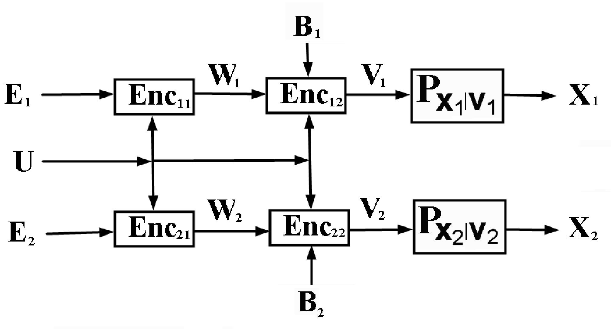
2. Encoding: Encode $c_{t}$ with encoder $t1$ and $t2$ (here $t=1$ or 2, refer to Fig. 2), according to the codebook generated in the previous step and obtain the codeword $v_{t}^{n}$. Then the transmitters generate the channel input sequences based on respective mappings $P_{X_{1}|V_{1}}$ and $P_{X_{2}|V_{2}}$. Actually this step is to apply artificial noise to $v_{t}^{n}$ according to the conditional probability distribution and get the transmitted signal. This step is to make the channel of the other receiver more noisy, and the intended receiver $t$ is supposed to know this $P_{X_{t}|V_{t}}$.

The encoder structure is illustrated by the following figure:

In the above figure, $U$ is the time-sharing sequence known by all the transmitters and receivers. The codebook for encoder $ij$ is denoted as $\lambda_{ij}\in\Lambda_{ij}$ ($i,j=1,2$), for the simplicity of notations, let $\lambda=(\lambda_{11},\lambda_{12},\lambda_{21},\lambda_{22})$, and $\Lambda=(\Lambda_{11},\Lambda_{12},\Lambda_{21},\Lambda_{22})$.

According to the structure of the encoder, we have the following relationship among the variables:

W_t^n = Λ(E_t^n, U^n), V_t^n = Λ(B_t^n, W_t^n, U^n)

3. Decoding: Without loss of generality, we consider for receiver 1. Let $A_{\epsilon}^{(n)}(W_{1},V_{1},W_{2},Y_{1},U)$ denote the set of jointly typical sequences defined in [17] page 521. Since receiver 1 is supposed to know the time sharing sequence $U^{n}$, after receiving $Y_{1}^{n}$, the receiver will try to find $\hat{W_{1}^{n}},\hat{V_{1}^{n}},\hat{W_{2}^{n}}$ such that $(\hat{W_{1}^{n}},\hat{V_{1}^{n}},\hat{W_{2}^{n}},Y_{1}^{n},U^{n})\in A_{\epsilon}^{(n)}(W_{1},V_{1},W_{2},Y_{1},U)$. When such choice exists and is unique then the decoding is successful, then message $E_{1}^{n}$ and $B_{1}^{n}$ can be restored, and the confidential message can be readily obtained by $f_{1}^{n}(E_{1}^{n},B_{1}^{n})$; otherwise declare error.

Part 2: Evaluation of Equivocation Rate

If we compare our modified scheme with the original one in [15], it can be easily observed that the decoding error probability in the new scheme is at least as good as the original one, which saves us the efforts to analyze the probability of decoding error. Hence we only need to show the existence of the tuple $(u,\lambda,f_{1}^{n},f_{2}^{n})$ such that the strong secrecy requirement (2), (3), (4) and (5) can be fulfilled. Without loss of generality, we just need to consider the information leaked to receiver 2 from sender 1. In [8], it has been proved that if $F_{1}^{n}$ is an uniform random variable on $\mathcal{F}_{1}^{n}$ and $\alpha_{1,\mathcal{I}}$ is the projection from $\mathcal{C}_{1}^{n}$ to $\prod_{i\in\mathcal{I}}\mathcal{C}_{1,i}^{n}$, then $\alpha_{1,\mathcal{I}}\circ F_{1}^{n}$ is a family of two-universal hashing functions. The projection is simply $\alpha_{1,\mathcal{I}}(C_{1}^{n})\triangleq\{C_{i,1}^{n}\mid i\in\mathcal{I}\}$. With a little abuse of notations, we also write $C_{1}^{n}=(F_{1}^{n})^{-1}(C_{1,1}^{n},\ldots,C_{1,T_{1}+1}^{n})$ (but the distinction can be made between the context compared with equation (33)), by the uniformness of the distribution it can be seen $C_{1}^{n}$ and $F_{1}^{n}$ are statistically independent.

We first calculate the mutual information $I(\alpha_{1,\mathcal{I}}(F_{1}^{n}(C_{1}^{n}));Y_{2}^{n}|F_{1}^{n},\Lambda,U^{n})$ averaged over all possible choices of $(u,\lambda,f_{1}^{n})$. Then by some probabilistic argument, the achievability of the theorem can be proved.

The following derivation is similar to [7] and [8], we first fix the code book $\lambda$ and the synchronization sequence $u$, and $\rho$ is a real constant with $0<\rho<1$.

where

We have the following relationship: $W_{t}^{n}=\Lambda(E_{t}^{n},U^{n})$ and $V_{t}^{n}=\Lambda(B_{t}^{n},W_{t}^{n},U^{n})$, thus

Take (38) into (35) and continue the derivation, we have

Then we average the above upper bound over $\Lambda$ and $U^{n}$:

References

• [1] Y. Liang, H. V. Poor, and S. Shamai (Shitz), Information Theoretic Security. Hanover, MA, USA: NOW Publishers, 2009.
• [2] R. Liu, I. Maric, P. Spasojevic, R. D. Yates, “Discrete memoryless interference and broadcast channels with confidential messages: Secrecy rate regions,” IEEE Trans. Inf. Theory, Vol. 54, No. 6, page 2493–2507, June 2008.
• [3] U. Maurer and S. Wolf, “Information-theoretic key agreement: From weak to strong secrecy for free,” in Proc. Eurocrypt, 2000, Lecture Notes in Computer Science, pp. 351–368.
• [4] D. Kobayashi, H. Yamamoto, and T. Ogawa, “How to attain the ordinary channel capacity securely in wiretap channels,” in Proc. 2005 IEEE Information Theory Workshop on Theory and Practice in Information-Theoretic Security, Oct. 2005, pp. 13–18, arXiv:cs/0509047.
• [5] R. G. Gallager. Information Theory and Reliable Communication. John Wiley & Sons, New York, 1968.
• [6] M. Hayashi. “Exponential decreasing rate of leaked information in universal random privacy amplification,” IEEE Trans. Inform. Theory, Vol 57, No. 6, page 3989–4001, June 2011, arXiv:0904.0308.
• [7] R. Matsumoto and M. Hayashi, “Strong security and separated code constructions for the broadcast channels with confidential messages,” 2011, arXiv:1010.0743.
• [8] R. Matsumoto, M. Hayashi, “Secure multiplex coding with a common message,” in Proc. ISIT 2011, Saint-Petersburg, Russia, Jul. 2011, page 1931–1935, arXiv:1101.4036.
• [9] R. Matsumoto, M. Hayashi, “Secure multiplex network coding,” in Proc. IEEE NetCod 2011, Beijing, China, Jul. 2011, page 24–29, arXiv:1102.3002.
• [10] J. Barros and M. Bloch. “Strong secrecy for wireless channels,” In R. Safavi-Naini, editor, ICITS 2008, volume 5155 of Lecture Notes in Compute Sciences, pages 40–53. Springer-Verlag, 2008.
• [11] U. M. Maurer. “The strong secret key rate of discrete random triples,” In R. E. Blahut et al., editors, Communications and Cryptography – Two Sides of One Tapestry, pages 271–285. Kluwer Academic Publishers, 1994.
• [12] X. He, A. Yener, “Interference channels with strong secrecy,” Proc. 47th annual Allerton Conference, page 811–818, Illinois, USA, Sep. 2009.
• [13] J. L. Carter and M. N. Wegman. Universal classes of hash functions. J. Comput. System Sci., Vol 18, No. 2, page 143–154, Apr. 1979.
• [14] A. B. Carleial, “Interference channels,” IEEE trans. Inf. Theory, Vol. 24, No. 1, page 60–70, Jan. 1978.
• [15] H.F. Chong, M. Motani, H.K. Garg, H.E. Gamal, “On the Han-Kobayashi region for the interference channel,” IEEE Trans. Inf. theory, Vol. 54, No. 7, page 3188–3195, July 2008
• [16] T. S. Han and K. Kobayashi, “A new achievable rate region for the interference channel,” IEEE Trans. Inf. Theory, Vol. 27, No. 1, page 49–60, Jan. 1981.
• [17] T. Cover and J. Thomas, Elements of Information Theory. New York: Wiley, 1991.