The non-perturbative renormalization group in the ordered phase.
Abstract
We study some analytical properties of the solutions of the non perturbative renormalization group flow equations for a scalar field theory with symmetry in the ordered phase, i.e. at temperatures below the critical temperature. The study is made in the framework of the local potential approximation. We show that the required physical discontinuity of the magnetic susceptibility at ( spontaneous magnetization) is reproduced only if the cut-off function which separates high and low energy modes satisfies to some restrictive explicit mathematical conditions; we stress that these conditions are not satisfied by a sharp cut-off in dimensions of space .
By generalizing a method proposed earlier by Bonanno and Lacagnina ( Nucl. Phys. B 693 (2004) 36.) to any kind of cut-off we propose to solve numerically the renormalization group flow equations for the threshold functions rather than for the local potential. It yields an algorithm sufficiently robust and precise to extract universal as well as non universal quantities from numerical experiments at any temperature, in particular at sub-critical temperatures in the ordered phase. Numerical results obtained for the potential with three different cut-off functions are reported and compared. The data confirm our theoretical predictions concerning the analytical behavior of at .
Fixed point solutions of the adimensionned renormalization group flow equations are also obtained in the same vein, that is by solving the fixed points equations and the associated eigenvalue problem for the threshold functions rather than for the potential. We report high precision data for the odd and even spectra of critical exponents for different cut-offs obtained in this way.
Keywords:
Non perturbative renormalization group; Local potential approximation; potential; Critical exponents; Numerical experimentspacs
02.30.Jr;02.30.Hq;02.60.Lj;05.10.Cc;11.10.Gh;64.60.F-I Introduction
During the last twenty years the non-perturbative approach to the renormalization group (RG) originated by Wilson [1, 2] has been the subject of a revival in both statistical and quantum field theory. Two main formulations of the non perturbative renormalization group (NPRG) have been developed in parallel to study a system at equilibrium at, or near to, criticality ; for instance, in the simplest case, a system described, at microscopic scale (in momentum scale), by an action where is a scalar field. In the first approach, one realizes a continuous RG transformation of the action from to and, a priori, no expansion with respect to whatsoever small parameter being required. At scale- (in momentum space) the high energy modes , , are integrated out in the “Wilsonian” action which is a functional of the slow modes , . This ”coarse-graining” operation requires the implementation of some cut-off of the propagator, either sharp or soft, aiming at separating slow () and fast () modes. This ”coarse-graining” process is devised in such a way that all the Wilsonian actions yield the same physics in the infra-red (IR) limit (). The flow of , from the microscopic scale to the macroscopic scale , is governed by the Wilson-Polchinski equation [1, 2, 3] in case of a smooth cut-off and the Wegner-Houghton [4, 5] equation in case of a sharp cut-off. Powerfull approximation schemes has been devised to obtain approximate, non-perturbative solutions of these equations; for a review see Ref. [6].
The second formulation, called the “effective average action” approach, was developed after the seminal works of Nicoll, Chang and Stanley for the sharp cut-off version [7, 8] and Wetterich, Ellwanger and Morris for the smooth cut-off version [9, 10, 11, 12]. This method implements on the effective average action - roughly speaking the Gibbs free energy of the fast modes , of the classical field - rather than on the Wilsonian action the ideas of integration of high-energy modes that underlies any RG approach. The flow of results in equations which can be solved under the same kind of non perturbative approximations than those used for the Wilson-Polchinski or Wegner-Houghton equations. The main advantage of this more recent formulation is that it gives access to the RG flow of physical quantities, i.e. the Gibbs free energy and its field derivatives, the vertex functions, rather than to such an abstract object as the Wilsonian action . Quite remarkably, the same kind of formalism was developed in a less elaborated language by Reatto et al. in the domain of the theory of classical liquids [13, 15, 14], many years before these recent contributions to statistical field theory. The relations between these corpora of works is discussed in ref. [16]. Recent reviews and lectures devoted to Wetterich’s approach are available [17, 18] and should be consulted for a thorough discussion. Wetterich’s version of the RG is in fact equivalent to that of Wilson-Polchinski as discussed in Ref. [12, 19].
In this paper we will adhere to Wetterich point of view and focus on the study of approximate solutions of the NPRG for a scalar field theory with symmetry, at a temperature below the critical temperature , i.e. in the “ordered phase” or “two phase region”. For the system exhibits a spontaneous magnetization which can take any value in the interval with an equal probability in the thermodynamic limit. Henceforth we shall reserve the name spontaneous magnetization for . As a result the susceptibility is infinite, or equivalently, the second derivative of the Gibbs free energy with respect to the magnetization
in the ordered phase. The potential , strictly convex for () is affine for .
The simplest non-perturbative version of the NPRG, i.e. the local potential approximation (LPA), yields indeed a convex free energy with a plateau as noticed in Refs [13, 15, 14, 17, 20]. However it has been discovered by Reatto et al. that the analytic behavior of in the vicinity of depends strongly on the choice of cut-off and dimension . For a sharp cut-off (and in ), is a continuous function of , notably at , and thus [13]. This is a serious flaw of the theory since obviously should be discontinuous at , i.e. vanishing identically in the two phase region with a jump to a finite positive value outside the two-phase region corresponding to a finite susceptibility. In other words one should have and . However, with another choice of cut-off function proposed by Litim [21], it was shown by Parolla et al. in Ref. [15] that, at least in , exhibits the correct discontinuity at . In this work we extend these results to any kind of cut-off and dimensions of space and obtain the mathematical properties to be satisfied by the cut-off function to obtain the required discontinuity of the susceptibility at . The crux of the whole matter is that the RG flow of Gibbs free energy stops in the ordered phase at some finite RG time and that the solutions of the RG flow can thus be obtained as asymptotic stationnary solutions for well chosen dimensionned functions the behavior of which gives insight on the region .
These analytical results are then checked by numerical experiments in the case of a potential where the RG flow equations are solved with a new algorithm which generalizes that devised by Bonanno and Lacagnina [20] to any kind of cut-off. The idea is to solve the RG flow for the threshold function rather than for the potential itself, or one of its derivatives. The partial differential equation for the threshold function is of quasi-linear parabolic type (rather than of non-linear parabolic type for the potential yielding huge numerical instabilities in the ordered phase) and can thus be solved with an arbitrary high accuracy. The approach to convexity of the Gibbs free energy is then achieved exactly with vanishing identically in the ordered phase, down to the smallest real available on your computer if wanted. Solving RG flow equations for the threshold function above is also possible of course, but of less interest. A good numerical precision can therefore be achieved making possible to extract precise universal as well as non-universal quantities from numerical experiments. Thorough numerical investigations have thus been undertaken with three different cut-off functions, i.e. the sharp cut-off, Litim’s regulator and an exponential smooth cut-off, aiming inter alia at testing the theoretical predictions on the behavior of at ; a thorough comparison and discussion of the data provided by the different cut-off is also presented.
This study is finally completed by solving the adimensionned flow equations asymptotically in the same vein as that used to solve the dimensionned equations, i.e. by solving the fixed point equations and the associated eigenvalue problem for the threshold functions rather than for the potential. Fixed point functions and critical exponents are then obtained for the three cut-offs with a very high numerical precision, notably for the exponential smooth cut-off non considered up to now; in the case of the sharp and Litim’s cut-off we recover the results obtained previously [22, 23].
The paper is organized as follows; in section II we summarize briefly Wetterich formalism and the LPA approximation. The properties of the RG in the two-phase region are then explored in depth yielding the mathematical conditions to be fulfilled by the cut-off function in order to obtain the correct discontinuous behavior of at . In section III we devise a new numerical algorithm in which a correct account of both initial and boundary conditions is given. This material is used to perform extensive numerical experiments aimed at testing the theoretical predictions of section II and at computing some universal and non-universal quantities of the potential. Section IV is devoted to a somehow new presentation and numerical study of the adimensionned flow equations. Estimations of the critical exponents of the (or Ising) model in the LPA and for three different cut-off are reported. In the case of Litim’s and sharp cut-off our results are in perfect agreement with those of ref.[22, 23] and in the case of the exponential smooth cut-off we provide the first high precision data for the even and odd spectrum of critical exponents. We conclude in Section V
II NPRG Flow equations in the local potential approximation
II.1 The model and the NPRG
We consider a scalar field theory defined at scale by it’s microscopic action
| (1) |
where is a scalar field defined at some point of the domain which encloses the system, ( dimensions of space.), symmetry is assumed (i.e. ) and we stick to the convention that brackets denote functionals while parenthesis are for functions. Below, for numerical applications, we shall restrict ourselves to the potential , i.e. a coarse-grained version of the Ising model with ( ), and will denote by the value of parameter at the critical point in the LPA approximation. Finally it is understood that acts as an ultra-violet (UV) cut-off in integrals defined in Fourier space, i.e. .
Following Wetterich [17] we introduce a family of related -models depending on an index in momentum space with . The bare action of the model - not to be confused with the Wilsonian action briefly alluded to in the introduction- is defined by
| (2) |
where is a massive term aimed at separating high and low energy field modes. is called the cut-off or regulator function. Translational invariance implies and the general behavior of the cut-off function is where is some positive prefactor accounting for field-renormalization and is some smooth approximation of the Heaviside step function so that when then . The cut-off functions must have the following generic behavior
- (i)
when , identically () and the original model is recovered.
- (ii)
when , is sufficiently ”large ” so that all the fluctuations are frozen by the massive term, i.e. the mean-field approximation becomes nearly exact.
- (iii)
when , is a decreasing function of which tends rapidly to for , thus the rapid modes are unaffected by the massive term. On the contrary the slow modes have a large mass which decouples them from the fast modes.
The physics of the k-systems is encoded in their partition functions
| (3) |
where the functional measure integrates over all the field modes () and ( source). At scale “k” the slow modes , , are frozen by their mass and can therefore be interpreted as the generator of the connected Green’s function with an IR cut-off. It is a convex function of the source and it’s Legendre transform defined as
| (4) |
is also a convex functional of the order parameter . is the “ true” Gibbs free energy of the k-system. However it proves convenient to introduce and consider rather the effective average action of Wetterich
| (5) |
By contrast with this functional of the field is non-convex but has simple limits which follow from the mathematical properties of the cut-off function [17], i.e. :
- •
when no fluctuations has been integrated out. and we will suppose that (mean field approximation).
- •
when all fluctuations have been integrated out and is the Gibbs free energy of the model under study.
Therefore when decreases from its initial value to all the fluctuations of the field are progressively integrated out and the effective action flows from the bare action (i.e. the mean-field approximation for ) to the Gibbs free energy of the model. The flow equation reads as [17]
| (6) |
where the inverse in the r.h.s. of Eq. (6) has to be understood in the operator sense, is the vertex function of order 2 and denotes is dimensional Fourier transform. Note that depends functionally on the field and the equation for is thus not closed. One has to resort to approximations to solve the flow.
II.2 The local potential approximation
A simple, non trivial way to tackle with Eq. (6) is to restrict the functional space to functionals of the form
| (7) |
which constitutes the popular local potential approximation (LPA). Note that in this scheme there is no field-renormalization so that . We also stress that the local potential is a function of the local field at point , not a functional. Combining Eqs. (6) and (7) one then obtains a closed partial differential equation (PDE) for the which reads as
| (8) |
where the potential is evaluated for a uniform magnetization and denotes its partial derivative with respect to . The PDE Eq. (8) is non-linear but however quite easy to solve numerically above the critical point (, in the case of the potential). Difficulties arise in the ordered phase. To understand why, we rewrite Eq. (8) under a more convenient form. We define the dimensionless variable , the RG time chosen to increases from 0 to when decreases from to 0, the dimensionless variable and the dimensionless functions of “y” : (so that ), , and so that
| (9) |
where and the threshold function (according to Wetterich terminology) is defined as
| (10) |
This function plays a central role in the mathematical analysis of Sec. II.3 and we need first to study its relevant analytical properties. For reasonable cut-off functions the two functions , and are positive for so that is a decreasing function of it’s argument. In any reasonable case the function is defined on the interval where is the largest pole of the integrand in the r.h.s. of Eq. (10) (for any reasonable choices of the cut-off there is in general only a single pole). Therefore decreases from to 0 when increases from to . Finally note that is indeed a dimensionless quantity which gives sense to Eq. (9).
Before we tackle the general case let us consider two important cases. First, the (ultra) sharp cut-off defined by the regulator where the parameter . In that case one shows that [17], so that the flow equation reads as
| (11) |
A second important case that we shall consider is Litim’s regulator which yields and the flow equation [21]
| (12) |
| = | 2.36806229624554475822396946574 |
|---|---|
| = | -3.83637249545350290077137812782 |
| = | 34.2450749455029367943794121780 |
| = | 26.7493978693695013104149308428 |
| = | -123.598329790226947089342622508 |
| = | 600.184183291720248551501270440 |
| = | 26.7493978693695013104149308428 |
| = | -4.62060231762294359247562464639 |
| = | .0406488093691634129962437962261 |
Let us consider now a regular smooth cut-off function. We have retained the exponential regulator widely used in recent numerical studies (see e. g. ref [24])
| (13) |
that is, written in reduced form , where is some positive parameter. It is easy to see that
- (i)
When the function , defined for , exhibits a single minimum at some and .
- (ii)
When the minimum of occurs precisely at and
- (iii)
When the minimum of on the interval is located at but .
The choice yields the better critical exponents according to the authors of reference [24] so we will retain this value; we are thus in the case (i) where the minimum of function is located at some non-zero value . We introduce . The threshold function is thus a monotonously decreasing function defined on the interval . Let us precise now its asymptotic behavior at each boundary of the interval.
Wetterich et al. [17] have shown how to obtain the behavior of for ; one expands around its minimum, i. e. , where and recognize the fact that, at the leading order,
| (14) | |||||
where
| (15) |
and .
Note that in Litim’s case one has , ; therefore the previous analysis breaks down and diverges as rather than as . In the case of the ultra sharp cut-off but the function is not well defined yielding a logarithmic divergence of as .
On the other hand an asymptotic behavior of for is readily obtained from (10) and reads
| (16) |
Since is bijective from to it can be inverted and we denote by its inverse. This function is defined on the interval where it decreases from to .
For we infers from (16) that
| (17) |
where
| (18) |
and for
| (19) |
The values of the constants are determined numerically; they are resumed in Table 1 in the case . For numerical applications the functions or , as well as their derivatives if required, have been fitted by polynomial expressions taking into account their asymptotic behaviors.
II.3 Flow equations for the threshold functions

As suggested first by Bonanno and Lacagnina [20] (however in a more restricted context) it is convenient to perform the change of variables with
| (20) |
The one to one mapping insures the mathematical equivalence of solving the RG flow equations either for or for . However, for numerical reasons the RG flow equation for is much easier to solve than that for [20]. The RG flow equation for is readily deduced from that for (cf. (9)) :
| (21) |
Eq. (21) is a quasi-linear parabolic PDE which can be studied analytically in some depth, notably in the two phase region, and for which, in addition, the mathematicians have provided us with robust and efficient solvers in view of a numerical study. For the exponential smooth cut-off (13) the function and its derivatives which enter Eq. (21) must be determined numerically. It is worthy to write down explicitely these flow equations
- •
for the sharp cut-off regulator ( and )
(22) - •
and for Litim’s regulator ( and )
(23)

II.4 Behavior of the flow in the ordered phase

Below , a spontaneous magnetization can settle in the system in the absence of an external magnetic field . More precisely, in the thermodynamic limit, any magnetization is likely to settle with the same probability. Roughly speaking we have a coexistence region of two (or more) magnetized phases analogous to a liquid-vapor coexistence. Therefore from which it follows that, in the limit the denominator of the r.h.s. of Eq. (8) tends to zero. Therefore the threshold function should become large and positive as and finally it should diverge to at for any magnetization in the two phase region .
With the hypothesis that is large and positive, as follows from (19); then the flow equation (21) for simplifies to
| (24) |
which can be integrated to give
| (25) |
for where is the constant of integration (depending on ) of Eq. (24). Clearly can be interpreted as a precursor of the magnetization of the system at scale . Note that can be obtained numerically from the numerical solution of PDE (21) from the value of at the origin. As expected one finds that for the function diverges to (recall that ) when as for any magnetization in the two phase region.
Outside the coexistence region -i.e. for - one expects a finite compressibility and thus tends to as with , as follows from (16). This behavior of is exemplified in figure 1 (details concerning the numerical procedure to solve (21) will be given in Sec. III).
One of the consequences of Eq. (25) is the universal behavior :
| (26) |
The function of the argument is thus universal as , i.e. it is independent of the thermodynamic state (provided the temperature satisfies ), the regulator , the value of , and the dimension of space . This remarkable features are illustrated in figure 2.
One can of course infer the behavior of the potential and its derivatives from that of and one has, for
| (27) |
where we have noted that for a symmetry; see figure 3 for an illustration. In the special case of the sharp cut-off and Litim regulator recall that one has to set in the above equations. Another interesting consequence of this simple behavior for the potential and its derivatives is the expression of the ”true” susceptibility of the k-system (cf Eq. (5)) which reads as
| (28) | |||||
and is thus positive at any . However the strict convexity of is preserved at each step of the RG flow in the LPA approximation only if as follows from the discussion after Eq. (12). Note that in that case Eq. (28) becomes . In the case , strict convexity could be violated and the validity of the LPA is no more guaranteed.
The simple behavior described by Eqs. (27) is independent of the regulator and has been known from long [14, 20]. However Parolla et al. [13, 15, 14] were the first to remark, in a more refined discussion, that the behavior of the susceptibility for depends strongly on the asymptotic behavior of for . For the sharp cut-off regulator they found that is continuous and equal to zero at (for ) (see Ref. [13]) while for the Litim regulator they found that, for , exhibits a discontinuity from a finite positive value at to a zero value at ( cf Ref. [15]). This discontinuity of the susceptibility jumping from an infinite value in the two phase region to a finite one outside, is of course the expected physical behavior for . In other words, in the case of the sharp cut-off regulator, the spinodal and the binodal curves merge in a single curve, which is a serious flaw in the theory (see figure 4).
We now extend the analysis of Parolla et al. to the quite general case :
| (29) |
where is an arbitrary exponent, not to be confused with the critical exponent of the correlation length! This expression includes notably the case of the exponential smooth cut-off considered in this paper - with , cf Eq. (14)- since only the singularity of as is relevant to study the behavior of as .

As follows from (25), when , diverges therefore to for for and tends uniformly to outside the interval (see fig. 1). This behavior is too “drastic” to discriminate the analytical properties of in the vicinity of . Borrowing an idea of Reatto et al. we introduce the following new function of the field
| (30) |
In the two phase region as and thus , while outside yielding to reach a finite value at . It follows from (25) and (30) that for and
| (31) |
We are led to introduce the new variable
| (32) |
such that, at fixed and for , one has
| (33) |
valid if , i. e. if . As quoted pleasingly by Parola et al.[13, 15] this variable allows us to “zoom“ in the region . Inside the two-phase region and we have the asymptotic behavior (33) of , while for , i. e. outside the the two-phase region, the function should reach a finite value . To avoid a proliferation of notations we still write the function expressed in terms of its new variables .
The dependence of the reduced spontaneous magnetization on as will prove of great importance in our analysis. A priori it should be reasonable to assume a k-dependence as
| (34) |
for sufficiently small ’s, since should be an analytical function of vector . Parameter describes the displacement of the precursor of the spontaneous magnetization with scale . With this reasonable assumption we can finally wrote the RG flow equation :
| (35) | |||||
We now analyse the asymptotic behavior of the stationary solutions () of EDP (35) at in the limit . This is justified since below the flow stops at some finite . These solutions are similar to scaling solutions at a fixed point; however and have dimensions and we cannot thus speak of scaling solutions stricto sensu. Obviously, in order to find these solutions, which we cannot refrain to christen as fixed point solutions despite our previous remarks, we have to discriminate our study according the sign of the exponent in Eq. (35).
II.4.1

Neglecting terms which tend to 0 when in Eq. (35) one finds the implicit fixed-point equation :
| (36) |
where . This is an autonomous differential equation which can be solved analytically :
| (37) |
where are integration constants, and a primitive of . We define as the integer part of , as its decimal part, i. e. , and we have
| (38) | |||||
where the third term in the r.h.s. of the equation is present only if and is the Lerch transcendent [25, 26]. This curiosity is defined on the disk (although it can be extended by analytical continuation to the cut plane ). It is defined as
| (39) | |||||
When is an integer Eq. (38) reduces to the simple form :
| (40) | |||||
This result was first obtain in Ref.[15] in the case (Litim case). From the known behavior of Lerch function, in particular for one deduces that
| (41) |
We are now in position to discuss the property of the fixed point solution Eq. (37). In the two phase region, , the function diverges to , thus , and one has asymptotically which fixes the value of the integration constant , from which we deduces . In the one phase sector, we find that reaches a finite value as . Returning to our old variables we have shown that the fixed point solution satisfies :
| (42) |
from which follows that for (and ) the susceptibility is discontinuous at . See Fig.(5) for an illustration.
II.4.2

We consider here the marginal case . It is an important one since it corresponds to the general smooth cut-off (, cf Eq. (14)) in . Neglecting terms which tend to 0 when in Eq. (35) one finds the implicit fixed-point equation :
| (43) |
This equation does not seem to have an analytical solution but, asymptotically :
| (44a) | |||||
| (44b) | |||||
Equation (44a) is required by the correct matching with the solution (33) in the two-phase region while (44b) guarantees finite susceptibility outside the magnetization curve. We conclude again in favor of a discontinuity of the susceptibility at . See Fig.(6) for an illustration.
II.4.3

In this case the term in ”a” which accounts for the displacement of the spontaneous magnetization with scale (cf Eq. (34)) can be discarded from Eq. (35). The function is no more adapted to our discussion and we are led to a new change of variables to eliminate the relevant dependence on from the RG flow equation. Let us introduce
| (45) |
By use of these variables the RG flow equation for admits in the limit a stationnary solution which satisfies the following differential equation :
| (46) |
This equation cannot be solved analytically but it satisfies the boundary conditions
| (47a) | |||||
| (47b) | |||||
Equation (47a) is required by the correct matching with the solution (33) in the two-phase region, while (47b) implies a non-physical divergence of the susceptibility on the magnetization curve. Indeed it follows from (47b) and (45) that ( since ) where the exponent
| (48) |
is strictly positive if . Not unexpectedly, one recovers, in the limit , the exponent obtained by Parolla et al. in the case of the sharp cut-off [13]. For the cut-off considered in this section the LPA seems to detect the spinodal rather than the coexistence curve and the exponent can be interpreted as the exponent of the inverse compressibility on the spinodal. Note that, however, it depends strongly on the non physical exponent which characterizes the divergence of the threshold function as .

We conclude that for (and and ) the LPA has the unphysical feature to give an infinite susceptibility at . The isotherm is continuous with and vanishes exactly in the two-phase region. See Figs. (7) and (8) for an illustration.
The conclusion of this section is that, if the singularity of the threshold function at is characterized by the exponent (cf Eq. (29)) and if , then
- •
For the inverse compressibility is continuous at , which constitutes a severe flaw of the theory.
- •
For the inverse compressibility is discontinuous at
III Numerical integration of the dimensionned RG flow equations
III.1 Algorithm
In order to solve the EDP (21) we must specify
- •
(i) an arbitrary initial condition at ()
(49) where is some maximum magnetization.
- •
(ii) boundary conditions
(50) where is some minimum value of the scale .
- •
(iii) The functions and a priori arbitrary must be such that [30]
(51)
Under these 3 conditions the RG flow equation for have a unique solution. The choice of and relies on physical grounds. At the cut-off function should diverge [17, 18] such that . Thus, clearly, must be imposed as an initial condition even if is not large enough so that is not actually infinite in the mathematical sense.
We propose to choose as boundary conditions the one-loop approximation for . Most authors usually adopt free boundary conditions. At a large fluctuations are frozen and the one-loop approximation should be pertinent. It is easy to see that at the one-loop level one has, up to an additional constant, independent of the field [27]
| (52) | |||||
from which it follows that :
| (53) | |||||
Therefore the one-loop approximation for reads as
| (54) |
To summarize we impose
- •
(i) initial condition : .
- •
(ii) boundary conditions .
and we stress that the compatibility condition (51) is obviously satisfied hence the RG flow equation can be solved safely at least from a mathematical point of view.
III.2 Numerical experiments

The RG flow equation (21), completed with the initial and boundary conditions of Section III.1, is a standard well-conditionned quasi-linear parabolic EDP which can easily be solved numerically. We adopted the fully implicit predictor-corrector integration scheme of Douglas and Jones [32] which proved to be very efficient and precise. Douglas and Jones have proved that their procedure leads to an unconditional convergence to the solution and that the truncation error is of order where is the discrete time-step and the grid-step for the field.
We limited ourselves to the potential with (arbitrary units) and being kept fixed while varying in order to make some contact with previous numerical studies [20]. This is a well acceptable choice of initial condition provided one does not want to describe nonuniversal characteristics of, e.g., the Ising model. The model was studied with the sharp, Litim and smooth cut-off regulators introduced in Section II.2. Some studies with the simplified smooth cut-off described by Eq. (29) with were also performed to compute in the vicinity of . Since no numerical simulations are available for this continuous version of the model we tried to extract from our data similarities as well as differences between the various versions of the LPA.
Typically we retained , after checking that the results were not influenced by the boundaries conditions. The time-step was typically and the field-step ranging from to according to the problem at hand. In all cases the integration of the EDP was stopped at some between and after checking that the solution did not evolve any more. Typically about time steps were necessary to reach convergence. For the smooth cut-off it was moreover necessary to fit the function defined as the inverse of function (cf Eq. (10)), its derivatives and inverse yielding unavoidable systematic errors and a reduction of the precision on the data.
III.2.1 Thermodynamic potentials below
We display in Fig. 1 the evolution of threshold function when the scale-k of the RG flow decreases from to . The curves have been obtained with Litim’s regulator; other approximations give similar curves, except the Sharp cut-off since can become negative in this case. The universal behavior (26) of the LPA is exemplified in Fig. 2 in the appropriate reduced variables.
The behavior of the potential which can be extracted from is displayed in Fig. 3. Note that the second derivative the true Gibbs potential of the k-system remains positive as we shown in sec II.4 (cf. Eq. (28)). For the considered state and at the lowest where we stopped the integration of the RG flow one finds and the inverse susceptibility jumps from at to at . Lowering the value of doe not change the value of the spontaneous magnetization (for a given grid step) while may be given any arbitrary small value for .
The approach to convexity is also well illustrated by the anti-clockwise rotation of the plateau of , i.e. the precursor of the magnetic field, towards an horizontal segment as in agreement with Eq. (27). Finally one notes that all the behaves as parabola inside the coexistence curve, according to Eq. (26), as soon as is sufficiently small.
III.2.2 Continuity/discontinuity of the susceptibility
Here we check numerically the conclusions of Sec II.4 concerning the continuity or discontinuity of the susceptibility at in the various versions of the LPA. Fig 4 displays the inverse susceptibility in the vicinity of for the sharp, Litim’s, and exponential smooth cut-off in dimensions. A relatively small field-step is required to be convinced of the (dis)continuity of the curves. Although such numerical checks cannot be retained as mathematical proofs stricto sensu, the theoretical predictions, i. e. continuity of at for the sharp cut-off and discontinuity for the Litim and smooth exponential regulator are quite well supported by the numerical outcomes.
Figs 5, 6, 7 and 8 display the curves obtained numerically in the case of the simplified smooth cut-off threshold function, i.e. for dimensions of space , , , and respectively. Recall that the behavior of any theory involving a smooth regulator is expected to be of that type. In all cases , and while the parameter of the potential has been adjusted for a spontaneous magnetization . For each dimension ”” we considered several values of field-step ranging from to corresponding resp. to a sampling of to points in the interval in order to emphasize the numerical difficulty to check this (dis)continuity. As expected (see Sec II.4 ) a spectacular change of behavior at . From continuous at low dimensions (cf the analysis of Sec II.4.1) becomes discontinuous for . Generally at most a single point seems to survive half the way the two discontinuity points whatever the tiny the value of considered. In particular note that, exactly at , “looks” indisputably discontinuous at as anticipated by the analysis of sect II.4.2.
III.2.3 Determination of the critical point and the critical exponents
It follows from Eq. (27) that the quantity is well suited to discriminate states at a temperature above from those at a temperature below . Indeed, as , diverges to at ( since the inverse compressibility is finite for ), while it tends to for subcritical states, ( cf Eq. (27)). A dicothomy procedure then yields the precise determination of the critical temperature as exemplifies by Fig.9 which displays results only for the ultra-sharp cut-off since in the other variations of the LPA (Litim’s or smooth cut-off) the bunch of curves is roughly similar and brings no new information. The results for are reported in table 2. For a given approximation they depend slightly on the field-step but as soon as is as small as we noted no effect on , up to its digit, by decreasing its magnitude. Note that we can ascertain exact digits on the value of from the data obtained with .
| (Litim) | (Sharp) | (Smooth) | |
|---|---|---|---|
| -0.1969317598 | -0.2971859571 | -0.4120948764 | |
| -0.1969322088 | -0.2971863642 | -0.4120953249 | |
| -0.1969322133 | -0.2971863684 | -0.4120953292 |
| Litim | Sharp | Smooth | |
|---|---|---|---|
| 0.3327(8) | 0.3532(9) | 0.3352(8) | |
| 1.2768(14) | 1.3292(26) | 1.2781(14) | |
| 0.0578(32) | -0.0356(44) | 0.0515(32) |
Quite noticeable is the dispersion of the values of corresponding to different cut-off functions which casts some doubts to the validity of the LPA to predict quantitative non universal results. This is an important detail that the non-universal parameters appear to depend strongly on the initial value considered at . If one changes something (a cutoff function for example), then the nonuniversal characteristics of the system changes. Moreover the MF approximation injected as an initial condition for the flow is a too crude approximation. From this respect our results are only but superficially at odds with those obtained recently by Dupuis and Machado for the Ising and lattice models where an excellent agreement (within a few percents) between the LPA prediction for and the MC data was found [29]. However in their work all these authors adopt a slightly modified version of the NPRG-LPA in which the effective action at is not taken as the mean field result but as the exact one (at this scale) and where integrations over the continuous momenta is replaced by a summation over the vectors of the first Brillouin zone. Similarly in the domain of the theory of liquids, the works reported by Reatto et al. attest good agreement between the LPA and the MC data [13, 15, 14]; in this case the exact physics of a reference system (the hard spheres fluid) is injected in the theory.
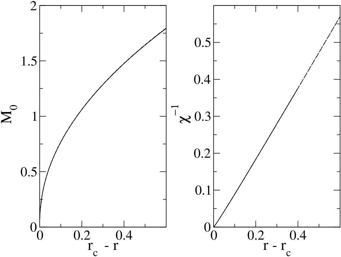
However when either the spontaneous magnetization (for ) or the inverse susceptibility (for ) are reported on a graph as functions of rather than versus all the curves obtained by means of different regulators collapse on a single, approximatively universal one, at least at large scale. This striking observation is exemplified in Fig. 10. In first approximation the effect of the cut-off seems to be a simple shift on . If we abandon the Sirius point of view and zoom in the vicinity of the various routes yield in fact different behaviors since the critical exponents differ slightly. A series of numerical experiments which are resumed in Fig. 11 allows a rough determination of the critical exponents of the magnetization -- and the susceptibility --. As apparent in Table III the values obtained for these two exponents in the case of the Litim and Smooth cut-off regulators are in good agreement but they differ quite significantly from those obtained for the sharp cut-off. By passing we note that Rushbrook’s equality yields a negative (exponent of the specific heat) in the case of the sharp cut-of, a well-known flaw of this approximation. A more stringent discussion will be given in next section where the exponents will be calculated with a high precision.
IV Integration of the adimensionned RG equations
.

IV.1 Adimensionned RG flow equations
In order to study fixed point solutions and the spectrum of critical exponents of the LPA we need to work with dimensionless potentials and fields. Since and we define the dimensionless magnetization and the dimensionless potential , so that the RG flow Eq. (9) takes now the form
| (55) |
in which the ’ designates a derivative with respect to . Further simplification can be obtained by introducing finally reduced variables. In the general case one defines and . Litim case will be our exception with the choice , and the redefinition valid henceforth . With these notations we have now in any case :
| (56) |
IV.2 Fixed points and exponents
Fixed point solutions and of Eqs. (56) and (57) resp. are peculiar solutions of the ordinary differential equations (ODE)
| (58a) | |||||
| (58b) | |||||
respectively. Note that if is a solution of Eq. (58a) then is a solution of Eq. (58b); similarly from a solution of (58b) one builds to get a solution of (58a). Because of the assumed symmetry we will consider only even solutions of Eq. (58a). Then, since , is also an even solution of Eq. (58b).
Once an even fixed point has been found (analytically or numerically) one investigates the behavior of the solutions of Eqs. (56) and (57) in the vicinity of this fixed point. As usual, we write and consider as small. Linearizing Eq. (56) with respect to leads to the eigenvalue equation :
| (59a) |
Similarly writing and linearizing the full RG flow equation with respect to yields.
| (59b) |
A first glance, since
the two spectra are identical and the eigenfunctions related by
| (60) |
Strictly speaking this is true only if is not identically equal to 0. Thus if it turns out that is either a constant or a linear function of then eigenvalue does not belong to the spectrum of the RG operator acting on . As well known, odd and even eigenvectors form two mutually orthogonal linear subsets and will be both considered in the sequel.
IV.3 Trivial solutions
Such trivial solutions exist whatever the type of fixed point; they are more easily detected on the eigenvalue problem (59a), i.e. that attached to the linearization of the RG about . Let us rewrite Eq. (58a) for as well as the equation for its derivative ; one has
| (61a) | |||||
| (61b) | |||||
Comparing these equations to the eigenvalue problem (59a) one readily sees that
- (i)
The constant is a trivial even eigenfunction of (59a) with the eigenvalue
- (ii)
- (iii)
with is another trivial odd eigenvector associated with the magnetic field.
From the remark of the previous section it follows that only the trivial odd eigenvalue survives in the eigenvalue problem (59a), i.e. that attached to the linearization of the RG flow about . According to (60) the corresponding eigenvector is the odd function .
IV.4 Gaussian fixed point
We show now that, provided that , the LPA admits a Gaussian fixed point, with the usual spectrum of exponents, irrespective to the type of cut-off. The fixed-point equation for , i.e. Eq. (58a), admits as a special solution. By integration it gives ( symmetry) and with ; where for the sharp and Litim’s cut-off respectively and, numerically, for our smooth cut-off. Obviously is the related special solution of Eq. (58b) provided .
The linearized eigenvalue problem for reads
| (62) |
where (cf for Sharp and Litim’s cut-off, while, numerically for the smooth-cut-off). The change of variables
| (63a) | ||||||
| (63b) | ||||||
allows to rewrite Eq. (62) as Hermite equation :
| (64) |
If we request the potential to be bounded by polynomials, must be restricted to an integer. Then Eq. (64) becomes the equation defining Hermite Polynomials . The parity of being that of , the spectrum of even eigenvalues is given by
| (65) |
with and . The trivial relevant operator with is indeed present in the spectrum as discussed in sec (IV.3). Whatever the type of cut-off we recover the well-known result : in we find one relevant operator ( with ), a marginal operator ( with ) and the first irrelevant operator with () while in there are two relevant operators ( and with and , respectively) and a marginal operator ( with ), while the first irrelevant operator is with . Some remarks are in order.
- •
An analysis similar to that of ref.[5] reveals that the marginal operators become irrelevant at the quadratic order.
- •
- •
The odd spectrum is given by , an integer. It includes the trivial solution . The other trivial odd eigenvalue is absent accidently from the spectrum, since it should correspond to a zero eigenvector ().
IV.5 Non Gaussian fixed point
In this section we focus on the non Gaussian fixed point in . Recently, the LPA fixed point equation for have been solved with a very high numerical precision for the sharp and Litim’s cut-off [22, 23]. Here we report numerical solutions for only in dimension ; the three cut-offs considered in this paper were examined and compared. Eq (58b) can be solved by the shooting method with boundary conditions imposed either at the origin or at [22, 23], hence the names given to the two methods considered below.
IV.5.1 ab origine

| Litim | Sharp | Smooth | |
|---|---|---|---|
| 0.122859820243702 | 0.61903040294652 | 7.355923051 | |
| -0.186064249470314 | -.46153372011621 | -.7995141985 | |
| 20.644305503116 | 94.128646935418 | 22.95208767 |
The LPA fixed point equation (58b) is a second order ODE for the function . Here we solve it numerically in by providing two initial conditions at . The first one, ensures the parity required by symmetry. It is now well-known that an arbitrary value of yields a solution singular at some finite value of the field. At we have for the Smooth or Litim’s cut-off and for the sharp cut-off. These singular values for correspond to . Actually, the general solution of (58b) involves a moving singularity of the form
| Smooth, Litim | (66a) | ||||
| Sharp | (66b) | ||||
where, in the case of Litim’s cut-off (the behavior near the singularity is driven by the asymptotics at infinity of the function , cf Eq. (16)). Figure 12 displays the variation of the singular point with the initial condition in the case of the Smooth cut-off (similar curves are obtained for the Sharp and Litim’s cut-off). Two peaks where diverges to can be noticed. The one on the left corresponds the Gaussian fixed point where is a constant with (see section IV.4). The one one the right corresponds to the Wilson-Fisher fixed point with that we are looking at..
Our requirement is that the physical solution must be non singular on the entire range so we must push to infinity by adjusting the value of by a dichotomy process in the vicinity of the right peak of figure 12 [33]. Of course high precision ODE solvers are required for this kind of study.
We solved equation (58b) as well as all the ODE of this paper with the DOPRI853 algorithm of Hairer et al. [31] which is an explicit Runge-Kutta integrator of order “8” and order “5” embedded, with adaptive step-size. We imposed relative and absolute errors of and respectively; the code was written in FORTRAN90 in quadruple precision. Even with this high technology it is impossible to obtain very large values of by tuning . Our results are summarized in Table 4. Our results for deduced of our result for agree within 14 figures with those of ref.[22, 23] in the case of Litim’s and sharp cut-off regulators. The data reported in Table 4 for the smooth cut-off are much less precise due to the use of fits for computing function . The complicated behavior of function is exemplified in fig. (13) (red curve); We displayed only the result for the smooth cut-off, Litim’s case is similar while for the sharp cut-off tends to at instead of “0”.
This ab origine method is rather deceptive but however usefull to check the data obtained by the ad originem shooting method that we discuss now.
IV.5.2 ad originem

The existence of a moving singularity at which seems impossible to “push“ at infinity suggests to solve Eq. (58b) with initial conditions at infinity, at least large, towards . The analysis of the asymptotic solutions of (58b) for shows the existence of power law solutions. This second family of solutions with regular scaling properties must obviously be preferred to the singular solutions discussed in section (IV.5.1). One can show that, asymptotically, for one has, for the smooth cut-off regulator
| (67a) | ||||
| with and an arbitrary coefficient. Recall that enters the asymptotic behavior (17) of as and are given in table 1. Litim’s case can be obtained from (67a) by the substitution , and . In the case of the sharp cut-off one has | ||||
| (67b) | ||||
In all cases the asymptotics depend on a single parameter which fixes the two initial conditions and at . is determined in such a way that . This is the shooting method ad originem.
| Litim | Sharp | Smooth | |
| 33.3250777220334 | .091029082436564 | 392.879344670467 |
The code DOPRI853 detects a stiff problem at large ”x“ so it is impossible to choose a very large value of . Actually we retained , and for Litim’s, the sharp and smooth cut-off regulators respectively. However taking into account the full asymptotic expansions(67a) or (67b) one recovers exactly, i.e. with all the significant figures reported in table 4 , the values of obtained by the shooting ab origine. The values of coefficient at the fixed point obtained by a dichotomy are given in table 5. Stiff integrators could be used instead of DOPRI853.
Figure 13 displays our results for (smooth cut-off case) obtained by the two shooting methods. At small ”x” both curves coincide quasi exactly up to some ; at two branches of the solution separate one that comes from the origin, the other, with scaling properties at infinity which comes from infinity. This hysteresis phenomenom cannot be discarded numerically.

From one deduce and thus the fixed point by integration (up to an additional constant). In private and informal discussions the opinion circulates that the histogram of the order parameter of the Ising model at its critical point should coincide with (up to normalization constants). We are not aware of any rigorous proof of this assertion but tentatively took it seriously. This histogram has been obtained by Monte Carlo simulations [34] and is compared in figure14 with the theoretical predictions of the LPA within the three versions considered in this paper. Note that all the histograms has been normalized in such way that the two first even moments are equal to unity, i.e. and . To inject some quantitative elements in the discussion of these curves we note that the kurtosis is experimentally, while in the LPA one finds , and for Litim’s, the sharp and smooth regulators respectively.
The behavior of at large deviations “” can also be obtained in the framework of the LPA by computing the asymptotics of the fixed point solution . Assuming a power law behavior as , Eq. (58a) is used to obtain
| (68a) | ||||
| with and a coefficient which enters at each order in the asymptotics (it’s value is such that ). Of course is related to the coefficient which governs the asymptotics of , one finds that . Recall finally that enters the asymptotic behavior (16) of as and are given in table 1. | ||||
Litim’s case can be obtained from (68a) by the substitution and while, in the case of the sharp cut-off, one has
| (68b) |
where, once again but .
IV.5.3 critical exponents
| Litim | Sharp | Smooth | |
|---|---|---|---|
| 1.539499459806177 | 1.450412451707412 | 1.53706 | |
| 0.649561773880648 | 0.689459056162135 | 0.650594 | |
| 0.655745939193339 | 0.595239852232561 | 0.654104 | |
| 3.180006512059168 | 2.838426658241768 | 3.17183 | |
| 5.912230612747701 | 5.184192105359884 | 5.55112 | |
| 8.796092825413904 | 7.596792580450411 | 8.76972 | |
| 11.798087658336857 | 10.057968960649436 | 11.7609 | |
| 14.896053175688298 | 12.556722422589013 | 14.8473 | |
| 0.4999999999999999 | 0.499999999999999 | 0.500004 | |
| 1.8867038380914204 | 1.691338925641807 | 1.88197 | |
| 4.5243907336707728 | 3.998514715824934 | 4.51219 | |
| 7.3376506433543136 | 6.382503789820088 | 7.31630 | |
| 10.2839007240259583 | 8.821709390384049 | 10.2522 | |
| 13.3361699643459432 | 11.302996690411253 | 13.2933 |
We turn now to the eigenvalue equation (59b). Again this is a second order ODE the solution of which is characterized a priori by two integration constants. Actually one of these is irrelevant and corresponds to the arbitrariness of the normalization of an eigenfunction. Since the fixed point solution is an even function of equation (59b) is invariant under a parity change and the spectrum separates into even and odd eigenvalues. The second integration constant is thus fixed by the choice (even) or (odd). The shooting ad originem method seems mandatory and one proceeds as in section IV.5.2.
For the smooth cut-off regulator the asymptotic behavior of the eigenfunctions as is found to be
| (69a) | ||||
| where is an arbitrary constant and . Imposing this form for at some large one tunes to obtain either or The case of the sharp cut-off is special : | ||||
| (69b) | ||||
| where . | ||||
Our results for the even and odd spectra are reported in table 6. In the even case there are no trivial eigenvalues, as shown in Sec. IV.3, and the first eigenvalue is related to the critical exponent of the correlation length of the Ising model. The first negative eigenvalue is minus the Ising-like first correction-to-scaling exponent and so-on. In the odd case, as discussed in Sec. IV.3 there are in general two positive trivial eigenvalues and , among which only the second one survives in the spectrum. The first non-trivial eigenvalue is negative and defines the subcritical exponent and so on.
The numerical data for serves as a stringent test for the precision of the numerical procedure; while (at least) significative digits are obtained for the sharp and Litim’s cut-off no more than digits can be ascertain in the case of the smooth cut-off. It originates in the various fitting procedures devised to evaluate the function and its derivatives. In the case of Litim’s and the sharp cut-off our results are in perfect agreement with those of ref.[22, 23]. Overall good agreement between the Litim and smooth cut-off spectra should be stressed.
Since in the LPA, one can compute all critical exponents from the critical exponent of the correlation length by the scaling relations. One has for : , , and . The values are reported in table 7. The comparison with the data of Table 3, obtained by solving the dimensionned PDE flow equation, is deceptive since there is no good agreement even by taking into account the error bars. The values obtained for ( ) by the numerical experiments of section III are systematically larger (smaller) than that obtained in this section. The explanation of this discrepancy relies probably in systematic errors due to the size of the field and time steps in the numerical resolution of the PDE.
| Litim | Sharp | Smooth | |
|---|---|---|---|
| 0.324780886940324 | 0.3447295280810675 | 0.325297 | |
| 1.299123547761296 | 1.37891811232427 | 1.301188 | |
| 0.051314678358056 | -0.068377168486405 | 0.048218 |
V Conclusion
In this paper we attempted to make an exhaustive study of the properties of the model in the ordered phase in the framework of the NPRG within the LPA approximation.
We shown that the approach to the convexity is independent of the cut-off, but that fine details are strongly affected by the choice of the regulator, notably the analytical behavior of the inverse magnetic susceptibility at . We proved that the singularity of the threshold function about its largest pole (or essential singularity) governs the behavior of at ; if as then the inverse compressibility is discontinuous at (as required on physical grounds) only if the inequality holds. In particular Litim’s and any smooth cut-off yield a discontinuity of in dimension , while the sharp cut-off incorrectly predicts a continuous behavior and thus a merging of the spinodal and binodal curves.
We have confirmed these subtle properties of the solution below by extensive numerical experiments with the help of a new algorithm which solves the RG flow equations for the threshold functions rather than for the potential or one of its derivatives. The main advantage of the method is to replace the numerical resolution of a highly non linear PDE which exhibits numerical instabilities in the ordered phase by that of a quasi-linear parabolic PDE with good convergence properties.
The ”standard” version of the LPA retained in this work does not allow to compute the critical parameter of the model which depends strongly upon the choice of cut-off. The main reason is that the choice of the MF approximation as an initial condition for the RG flow is a too crude approximation. Modified versions of the NPRG [13, 15, 14, 19, 29] remedy to this flaw and yield a quite precise estimate for . However we noticed that, choosing as a new variable instead of , the thermodynamics of the LPA (spontaneous magnetization, magnetic susceptibility) for the potential is remarkably independent of the cut-off, except very close to the critical point. The latter merely shift to incorrect values. The numerical solution of the dimensionned RG flow equation does not yield a very precise estimate of the critical exponents either, probably because of small numerical errors in the resolution of the PDE.
In order to compute precisely the critical exponents one must solve the linearized RG about the Fisher fixed point. It can also be done for the threshold functions instead of the potential or its derivatives without any noticeable numerical differences but with the advantage of getting rid of some trivial solutions corresponding to redundant operators. The solution of the resulting fixed point equations and associated eigenvalue problems can be obtained with a high numerical precision with the help of a non-stiff solver like DOPRI853 [31] for instance. Since the ad originem problem is stiff, stiff integrators could be of some help however to reduce the integration step and should be tested.
It is not clear whether the LPA scenario for the ordered phase survives for more elaborate approximation schemes, this could be the subject of further investigations.
Acknowledgements.
The author would like to thank personally C. Bervillier for enlightening e-mail correspondence, notably sec. IV.3 owes much to his remarks, and, collectively, all the members of the “groupe de travail NPRG” of the LPTMC (Jussieu, Paris), directed and animated by G. Tarjus, for many discussions. The anonymous referee of this paper is acknowleged for many pertinent remarks on the manuscript.References
- [1] K. G. Wilson, J. Kogut, Phys. Rep. C 12 (1974) 77.
- [2] F. J. Wegner, Phase Transitions and Critical Phenomena Vol. VI, C. Domb and M. S. Green eds., Academic Press, New York, 1976.
- [3] J. Polchinski, Nucl. Phys. B 231 (1984) 269.
- [4] F. J. Wegner and A. Houghton, Phys. Rev. A 8 (1972) 401.
- [5] A. Hasenfratz and P. Hasenfratz, Nucl. Phys. B 270 (1986) 687.
- [6] C. Bervillier, C. Bagnuls, Phys. Rep. 348 (2001) 91.
- [7] J. F. Nicoll, T. S. Chang, H. E. Stanley, Phys. Rev. Lett. 33 (1974) 540; ibid, Phys. Rev. A 13 (1976) 1251.
- [8] J. F. Nicoll, T. S. Chang, Phys. Lett. A 62 (1977) 287.
- [9] C. Wetterich, Nucl. Phys. B 352, (1991) 529.
- [10] C. Wetterich, Phys. Lett. B 301 (1993) 90.
- [11] U. Ellwanger, Z. Phys. C 62 (1994) 63.
- [12] T. R. Morris, Int. J. Mod. Phys. A 9 (1994) 2411.
- [13] A. Parola, D. Pini and L. Reatto, Phys. Rev. E 48 (1993) 3321.
- [14] A. Parola and L. Reatto, Adv. Phys. 44 (1995) 211.
- [15] A. Parola, D. Pini and L. Reatto, Mol. Phys. 107 (2009) 503.
- [16] J.-M. Caillol, Mol. Phys. 104 (2006) 1931; ibid, Mol. Phys. (to appear)
- [17] J. Berges, N. Tetradis, C. Wetterich, Phys. Rep. 363 (2002) 223.
- [18] B. Delamotte, Order, Disorder and Criticality. Advanced Problems of Phase Transition Theory, Vol. II, Y. Holovatch ed., World Scientific, Singapore, 2007.
- [19] J.-M. Caillol, J. Phys. A : Math. Gen. 42 (2009), 225004.
- [20] A. Bonanno, G. Lacagnina, Nucl. Phys. B 693 (2004) 36.
- [21] D. Litim, Phys. Lett. B 486 (2000) 92.
- [22] C. Bervillier, B. Boisseau, H. Giacomini, Nucl. Phys. B 789 (2008) 525.
- [23] C. Bervillier, B. Boisseau, H. Giacomini, Nucl. Phys. B 801 (2008) 296.
- [24] L. Canet, B. Delamotte, D. Mouhanna and J. Vidal, Phys. Rev. D 67 (2003) 065004.
- [25] I. S. Gradshteyn, I. M. Ryzhik Tables of Integrals, Series, and Products, (New-York, Academic Press (4th ed.) 1965); (see Chapter 9.55)
- [26] M. Lerch, Acta Mathematica 11 (1887) 1.
- [27] J. Zinn-Justin, Quantum Field Theory and Critical Phenomena, (Oxford: Clarendon Press,1989).
- [28] F. J. Wegner, J. Phys. C:Solid State Phys. 7 (1974) 2098.
- [29] T. Machado and N. Dupuis, Phys. Rev. E 82 (2010) 041128.
- [30] W. F. Ames, Numerical Methods for Partial Differential Equations (Academic, London, 1977).
- [31] E. Hairer, S. P. Nørsett and G. Wanner, Solving ordinary Differential Equations I (Springer, corrected 3rd printing 2008).
- [32] J. Jr. Douglas and B. F. Jones, J. Soc. ind. appl. Math 11 (1963) 195; See also ref. [30] (Chapter 2.14).
- [33] G. Felder, Comm. Math. Phys. 111 (1987) 101.
- [34] M. M. Tsypin and H. W. J. Blöte, Phys. Rev. E 62 (2000) 73.