Parity and reality properties of the EPRL spinfoam

The vertex amplitude $A_{v}$ as a function of $SU(2)$ elements $h_{l}$ on its surrounding graph is given by [13]:

where we made the dependence on $\gamma$ explicit in the notation. $n$ labels the graph’s nodes, $l$ labels the links, and $s(l),t(l)$ are the source and target nodes of the link $l$. As usual, for a graph with $N$ nodes, we integrate over just $N-1$ Lorentz group elements $g_{n}$, with the remaining one fixed to the identity in order to make the integral finite. In this subsection, we will show that $A_{v,\gamma}=A_{v,-\gamma}$. For this purpose, it’s convenient to think of the integration variables in (3) as actual $SL(2,\mathbb{C})$ (or $SU(2)$) matrices, rather than abstract group elements. To streamline notations, we introduce a symbol for the $J$-conjugate of an $SL(2,\mathbb{C})$ matrix:

where the $J$ in the second expression is the standard parity operation on 2-spinors. The operation (4) preserves the multiplication order and the Haar measure, and leaves $SU(2)$ matrices unchanged. It can be interpreted as either a $P$ or a $T$ reflection of the Lorentz rotations.

The inequivalent $SL(2,\mathbb{C})$ matrices are fully characterized by their complex trace. In its eigenframe, such a matrix is seen to consist of a spatial rotation and a boost in the perpendicular plane. The trace then encodes the rotation angle and the boost parameter. The complex conjugate of a given trace encodes (for instance) the same rotation with the opposite boost. Intuitively, this corresponds to a symmetry of the unitary Lorentz reps:

We will use below a special case of this relation:

Let us present a short proof of (6). The equivalence of matrices with equal traces will then imply the general relation (5). The $(p,j)$ representation of $SL(2,\mathbb{C})$ is given by functions of a 2-spinor $z$ with the homogeneity property:

with the group action and the Hilbert product defined by:

The integral is over non-collinear spinors $z$, and the two-form measure $\Omega$ is defined as:

where $z_{0}$ and $z_{1}$ are the two components of $z$. Note that $\Omega$ is real. Now, consider the representation obtained by acting with the matrices $g^{J}$ instead of $g$:

We claim that this new representation is in fact the $(-p,j)$ representation under a change of variables. To see this, define a new set of homogeneous functions $\tilde{f}(z)\equiv f(Jz)$. The expression (9) for the Hermitian product is invariant under $z\rightarrow Jz$ (the 2-form (10) picks up a minus sign, but this is canceled as usual by a reversal of the integration interval). In terms of $Jz$, the transformation law (11) takes the form:

Therefore, the functions $\tilde{f}(z)$ transform under the canonical rule (8). Finally, the homogeneity of $\tilde{f}(z)$ is obtained from (7) by interchanging $\lambda$ and $\bar{\lambda}$. The result is the homogeneity rule of the $(p,-j)$ representation. We conclude that the action of $g^{J}$ on the $(p,j)$ representation elements $f$ is isomorphic to the action of $g$ on the $(p,-j)$ representation elements $\tilde{f}$. As is well known, the $(p,-j)$ representation is isomorphic to the $(-p,j)$ representation, so eq. (6) follows.

Coming back to the vertex amplitude (3), let us perform a change of integration variables at the nodes:

This does not affect the Haar measure, or the fixing of one of the $g_{n}$ to the identity. Therefore, $dg_{n}\rightarrow dg_{n}$. Since $k_{l}=k_{l}^{J}$, the argument of the $SL(2,\mathbb{C})$ character in (3) transforms as:

Using (6), this implies:

Since the entire operation was just a change of integration variables, we obtain the result:

In [12], the vertex amplitude for a semicoherent state with spins $j_{ab}$ and spinor parameters $\xi_{ab}$ is written as:

where $n$ labels the graph’s nodes, $l$ labels the links, and $a,b$ label the source and target nodes of each link. $(-1)^{\chi}$ is a global sign factor from combinatorics, and the “link propagator” $\tilde{P}_{ab}$ is given by:

We refer the reader to [12] for a full explanation of this expression. The integral is performed over 2-spinors $z_{ab}$ with the measure $\Omega$ from (10). The $Z$ spinors are a shorthand notation for $Z_{ab}=g_{a}^{\dagger}z_{ab}$ and $Z_{ba}=g_{b}^{\dagger}z_{ab}$. The angle brackets stand for the Hermitian inner product in $\mathbb{C}^{2}$, and the norms $\|Z\|$ are defined with respect to that inner product. The phase factor $c_{ab}$ is given by:

We set $p_{ab}=\gamma j_{ab}$, which makes all the $c_{ab}$’s equal:

Note the asymmetric treatment in (27) of the link’s source and target nodes $a$ and $b$. We may interchange them by using the symmetry property of the $\beta$ form [12]:

We then have:

Now consider the change of integration variables:

The $dg_{n}$ and $\Omega$ integrals are invariant under these changes; so is the fixing to the identity of one of the $g_{n}$. The induced change in $Z_{ab}$ and $Z_{ba}$ is:

This turns (32) into:

This is the same as $P_{ab}$, except for the sign on $JZ_{ba}$ and an inversion of the $(\|Z_{ba}\|/\|Z_{ab}\|)^{2ip_{ab}}$ factor. This last difference corresponds to flipping the sign of $p_{ab}$, or equivalently of $\gamma$. Keeping in mind also the dependence of $c_{ab}$ on $p_{ab}$, we get:

The sign factor cancels nicely with the one in (31), giving:

where $L$ is the number of links in the graph. There is a discrepancy between the symmetries (37) and (16). It suggests that the vertex amplitudes (3) and (26) are not quite the same. Since (16) is a cleaner symmetry, it appears sensible to adopt a version of the semicoherent amplitude (26) that respects it. This amounts to omitting the $c_{ab}$ factors in (26)-(27) and defining:

This is the definition that we’ll adopt in the numerical analysis below. As we’ll see in section III.4, the omission of the $c_{ab}$ factors also leads to a more symmetric relation between parity-related amplitudes at fixed $\gamma$.

The work reported in this section began with the hope that the vertex is not invariant under $\gamma\rightarrow-\gamma$. Then a modified vertex of the form $A_{v,\gamma}+A_{v,-\gamma}$ could have resolved the chirality problems. As we’ve seen, this is not the case, and the proposed modification is trivial.

One may consider an alternative modification, which we now briefly discuss. $\gamma$ is traditionally taken to be a global parameter. However, its actual usage in the vertex amplitude (3) or (38) is to raise the representations on each link from $SU(2)$ to $SL(2,\mathbb{C})$ - an operation which can be considered for each link separately. In particular, we can imagine using different signs of $\gamma$ on different links. To restore the symmetry between the links, we must then sum over all $2^{L}$ such possibilities.

The arguments of subsections II.1-II.2, which demonstrated invariance under a global flip of $\gamma$, no longer apply. Therefore, this “per-link” flipping of $\gamma$ may be a genuine and interesting modification of the model. However, we must note that in the large-spin limit studied in [12], it degenerates back to the “global” flip $A_{v,\gamma}+A_{v,-\gamma}$. Indeed, it was shown in [12] that to avoid exponential suppression, $p_{ab}$ must be proportional to $j_{ab}$ with the same coefficient on all the links. Therefore, mixed terms with $\gamma$ on some links and $-\gamma$ on the others won’t contribute to the asymptotic amplitude.

We now turn to the parity structure of the large-spin 4-simplex amplitudes. We wrote a numerical script for the task. The script works with the semicoherent states described in [12], but without the $c_{ab}$ phase factors as we discussed in section II.2. The script is used to generate appropriate boundary-state parameters $(j_{ab},\xi_{ab})$ from simpler geometric data, to find the two critical points $(g_{a},z_{ab})_{\pm}$ for the transition amplitude, to calculate the Hessian of the “action” at these points, and finally to calculate the “semicoherent” piece of the graviton propagator.

In the Euclidean calculation of the graviton propagator [7], the authors used a regular 4-simplex for maximal symmetry. In a Lorentzian signature, a regular 4-simplex doesn’t exist. We therefore work with the next most symmetric possibility, i.e. an isosceles 4-simplex. It’s composed of a regular “base” tetrahedron in the $t=0$ hyperplane centered at the origin, and 4 isosceles “side” tetrahedra whose apexes meet at a point $(h,0,0,0)$. In turn, each of the isosceles tetrahedra is composed of a regular base triangle (where they touch the base tetrahedron) and 3 isosceles side triangles (where they touch each other). The base tetrahedron is labeled as node no. $0$, and the side tetrahedra are labeled as nodes $1\dots 4$.

Figure 1 depicts (in one fewer dimension) the location of the tetrahedra in the “source” 3d space, where the boundary state is defined. Here again, the base tetrahedron is centered at the origin. The side tetrahedra have a smaller height, and are glued to the base tetrahedron’s faces from the inside (see section III.3 on this point). The $SL(2,\mathbb{C})$ rotation matrices $g_{a}$ at the two critical points leave the base tetrahedron intact, while the side tetrahedra are boosted around their base triangles until their side triangles and apexes meet. The difference between the two critical points is that one boosts the side tetrahedra into positive $t$, and the other into negative $t$.

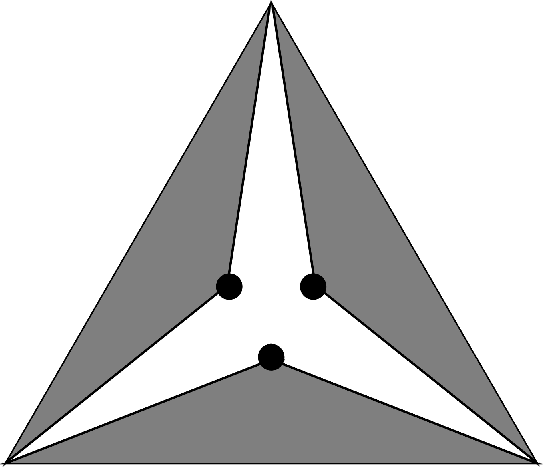
We note that exchanging two tetrahedra among the equivalent set $1\dots 4$ amounts to a parity-odd isometry on the 4-simplex. For instance, we can (and do) choose 4d axes so that tetrahedra $0,3,4$ are centered on the $z=0$ hyperplane, while tetrahedra $1,2$ are centered at opposite values of $z$. Then the exchange $1\leftrightarrow 2$ corresponds to the parity-odd isometry $z\rightarrow-z$. This correspondence between parity and the exchange of two tetrahedra will play a crucial role in the analysis of the graviton propagator in section III.5.

In this subsection, we describe the logical flow of the numerical calculation. Several details more related to programming than to geometry are deferred to the Appendix.

The recipe for semiclassical amplitudes in [12] begins with the parameters $(j_{ab},\xi_{ab})$ of the boundary state. These are then translated into a discrete 4-simplex geometry by the critical points of the integrals (38), if the boundary parameters admit such critical points. The geometry at the critical points may be Euclidean, Lorentzian or degenerate (i.e. effectively 3-dimensional). In the present context, our goal is slightly different. We wish to start with a boundary state which corresponds to a Lorentzian 4-simplex, and use this as a background for the graviton propagator. Therefore, the calculation works “backwards”: we start by specifying the desired geometry of the Lorentzian 4-simplex at the critical points, and calculate from that the required parameters $(j_{ab},\xi_{ab})$ of the boundary state.

The vertex positions of the base tetrahedron are hard-coded into the script. Its edge length is normalized to 1. This is the only hard-coded geometric data. All the rest is calculated dynamically in order to minimize human error, in particular with regard to signs and orientations. The script accepts as an input the rapidity with which the side tetrahedra are to be boosted at the critical points. From this we calculate their height and locations in the 3d source space, i.e. their vertex coordinates prior to boosting.

Once the coordinates of the tetrahedra are known, the parameters $(j_{ab},\xi_{ab})$ of the boundary state are calculated, following the prescription of [12] in reverse (up to the caveat in section III.3). We take the spins $j_{ab}$ to simply equal the corresponding triangle areas. The normalization is irrelevant for our purposes, and no harm is done by the non-half-integer values - in the stationary-phase limit, only the relative sizes of the spins matter. For $a<b$, we choose arbitrarily the phase of $\xi_{ab}$ according to the convention $(e^{-i\varphi/2}\cos(\theta/2),e^{i\varphi/2}\sin(\theta/2))$. The phase of $\xi_{ba}$ is then determined geometrically by the prescription in [12].

We calculate the rotation matrices $g^{\pm}_{a}$ at the critical points from the geometry of the 4-simplex. The critical values $z^{\pm}_{ab}$ of the $z_{ab}$ spinors are then determined from the first critical-point equation in [12], with the second component of each spinor normalized to 1.

The major task, and the one which drove us to a numerical treatment in the first place, is to calculate the Hessian $H$ of the “action” $S$ [12] at the two critical points. For that purpose, we must first encode the integration variables $(g_{a},z_{ab})$ into a set of $24+20=44$ non-redundant real quantities. Also, it’s useful to choose these quantities so that the Haar and $\Omega$ measures become trivial around the critical points. We do this as follows. For the rotation matrices, we first note that only 4 of them should be integrated over. We therefore keep $g_{0}=1_{2\times 2}$, and encode only the four others. For each of those, we encode not $g_{a}$ itself, but the matrix $\tilde{g}_{a}=g_{a}(g^{\pm}_{a})^{-1}$, which represents the deviation from the critical point. As the 6 independent real components of $\tilde{g}_{a}$, we use the real and imaginary parts of $((\tilde{g}_{a})_{01}+(\tilde{g}_{a})_{10})/2$, $i((\tilde{g}_{a})_{01}-(\tilde{g}_{a})_{10})/2$ and $(\tilde{g}_{a})_{00}$. Near the identity, these correspond to the Cartesian components of the rotation and boost generators, which ensures even spacing under the Haar measure. To encode the $z_{ab}$ spinors, we simply use the real and imaginary parts of $(z_{ab})_{0}$, after normalizing $(z_{ab})_{1}$ to 1.

With these ingredients in place, we calculate the Hessian by straightforward numerical differentiation. We will use the determinant of $H$ for the relative weights of the critical points in the amplitude, and its inverse for the graviton propagator.

We next calculate the gradients of the metric insertion functions $q_{n}^{ab}$ for $a,b\neq n$ at the two critical points. The prescription for the metric insertions is taken from [8], with two trivial modifications: to accommodate for all the cases $a<b$, $a=b$ and $a>b$, and to correct for the $ab\leftrightarrow ba$ discrepancy in conventions between [8] and [12]. This results in the following formula for $q_{n}^{ab}(g_{a},z_{ab})$:

where $\vec{\sigma}$ are the Pauli matrices.

At each of the two critical points, we contract the gradients of $q_{n}^{ab}$ with the inverse Hessian to obtain the semicoherent graviton propagator:

The propagator component $G_{mn}^{(ab)(cd)}$ represents the correlator between the metric elements $\underline{ma}\cdot\underline{mb}$ and $\underline{nc}\cdot\underline{nd}$. The indices $i,j$ in (43) run over the independent components of $(g_{a},z_{ab})$.

Two caveats are in order. First, the script only handles the case $m\neq n$ and $a,b,c,d\neq m,n$, when the double metric insertion is simply given by the product of two single insertions. Second, as mentioned in the Introduction, the quantity that we’re computing is not the full graviton propagator, but only its “semicoherent” piece. The full propagator would have been obtained from a fully coherent boundary state, with a weighted sum over spins. This sum would pick just one of the two critical points, and add a contribution to (43) from the derivatives with respect to $j_{ab}$. In fact, this contribution is the one containing the standard Regge propagator. We ignore it in the present context, because we are interested in parity violation, and that comes from the derivatives with respect to $(g_{a},z_{ab})$. Thus, we are calculating only the potentially troublesome part of the propagator. It can be cleanly separated from the $j_{ab}$-derivatives contribution, due to the vanishing of the Hessian elements $H_{jg},H_{jz},H_{j\bar{z}}$ [8].

We stress that all of the above can be done analytically. In particular, numerical differentiation is not necessary: not only the relevant functions, but also their derivatives are worked out analytically in [8]. The virtue of the numerics in this case is purely tactical - it provides a shortcut to some basic answers, allowing us to avoid tedious and error-prone derivations. Also, it will be able to provide a useful check for future analytical results. In fact, the hands-on numerics has already helped us uncover a minor problem in earlier analytical work, as we now describe.

The critical-point equations on $(g_{a},z_{ab})$ do not have solutions for generic boundary states $(j_{ab},\xi_{ab})$. In order to correspond to a semiclassical Regge geometry, the boundary-state parameters must satisfy certain constraints. These constraints have a geometric interpretation, as described respectively in [11] and [12] for the Euclidean and Lorentzian models. In the Euclidean, the $\xi_{ab}$ should be understood as the spinor “square roots” of the outgoing face normals of the tetrahedra, embedded in 3d space. Then the critical-point solutions correspond to folding these tetrahedra into a 4-simplex using 4d rotations. The same procedure was then carried over to the Lorentzian model in [12]. As we noticed while looking for critical points in the numerics, there is in fact a subtle difference between the two cases which must be taken into account.

For concreteness, consider the isosceles 4-simplex described in sections III.1-III.2. In the Euclidean model, its tetrahedra can be embedded in 3d space as a four-pointed “star”: the base tetrahedron is situated at the center, with the side tetrahedra glued to its faces from the outside. To fold this into a 4-simplex, the side tetrahedra must be rotated along their heights into the 4th dimension by some obtuse angle. Now, in the Lorentzian case such a rotation is not continuous with the identity: it would require passing through null and timelike configurations. In other words, it isn’t part of $SL(2,\mathbb{C})$. To fix this, we must glue the side tetrahedra to the inside of the base tetrahedron, as in figure 1. That way, they can be folded together by a finite boost.

Now, the critical-point equations in [12] require the spinors $\xi_{ab}$ and $J\xi_{ba}$ to point in the same direction after the 4d rotations. In other words, $\xi_{ab}$ and $\xi_{ba}$ should point in opposite directions. This is the case in the Euclidean setup, with all the $\xi$’s pointing along the outgoing normals of their respective tetrahedra. However, now that we took the side tetrahedra to lie inside the base tetrahedron, the base and side outgoing normals are parallel rather than antiparallel. This can be cured by taking the $\xi$’s for the side tetrahedra (or the base tetrahedron) to point along the ingoing normals to their respective faces.

This conclusion can be generalized to arbitrary Lorentzian 4-polytopes with spacelike boundaries. The boundary polyhedra can be classified according to the time-orientation of their outgoing 4d normal (not to be confused with the face normals discussed above). In constructing the semiclassical boundary state, we must take the $\xi$ spinors for the past-pointing polyhedra (say) to point along the outgoing face normals, and for the future-pointing polyhedra - along the ingoing face normals. This was the prescription we used in the numerical script.

In [12], the asymptotic analysis of the Lorentzian 4-simplex amplitude (with Lorentzian critical points) ends with the following expression:

where the sign factor comes from combinatorics, and $S_{Regge}$ is the Regge action:

with $\Theta_{ab}$ the dihedral angles (actually, boost parameters). The coefficients $N_{\pm}$ of the two parity-related critical points are given by:

where the piece in the second parentheses is the one which depends on the critical point. We again omitted the $c_{ab}$ phase factors, as discussed in section II.2. The authors of [12] left the ratio $N_{+}/N_{-}$ as an open question. We studied this question using the numerical script. Specifically, the script calculates the quantity $\left(\sqrt{\det H}\prod\|Z_{ab}\|^{2}\|Z_{ba}\|^{2}\right)^{-1}$ at the two critical points, keeping in mind that the $\Omega$ measure is trivial in our conventions. The numbers point clearly towards the simple result:

In other words, the amplitude (44) is real. In particular, the magnitudes $|N_{+}|=|N_{-}|$ are equal. Furthermore, at small $\gamma$ we have:

Here and below, we present extrapolations from numerical results as exact analytical relations. In all such cases, what’s actually implied is that the LHS and RHS agree to an accuracy of several digits, for a representative sample of points in the parameter space.

The results (47)-(48) may be compared with the Euclidean situation [11], where the coefficients of $\exp(iS_{Regge})$ and $\exp(-iS_{Regge})$ are equal for arbitrary $\gamma$ (and two additional terms appear). Note that the simple relation (47) is sensitive to the overall phase of the boundary state. It holds when the overall phase of $\xi_{ab}$ and $\xi_{ba}$ is fixed by the 3d rotation which makes the corresponding triangles congruent, as prescribed in [12]. The result is also dependent on our omission of the $c_{ab}$ phase factors in (38) and (46).

As a cross-check, the numerical results for $N_{\pm}$ confirm the $\gamma\rightarrow-\gamma$ symmetry claimed in section II. Concretely, the identity $N_{\pm}(\gamma)=N_{\mp}(-\gamma)$ is seen to hold.

Our main object of interest is the graviton propagator, in particular its parity-related components. More specifically, as discussed in section III.2, we are calculating the “semicoherent” propagator (43), where the summed indices $i,j$ run over the independent components of $(g_{a},z_{ab})$ and not over the spins $j_{ab}$. We calculate the quantity (43) at the two critical points separately, noting that only one will remain after the sum over spins. Also, we reiterate that (43) is valid only for $m\neq n$ and $a,b,c,d\neq m,n$.

As a first result of this calculation, we again see a confirmation of the $\gamma\rightarrow-\gamma$ symmetry, i.e. $G_{mn}^{(ab)(cd)}(\gamma)=G_{mn}^{(ab)(cd)}(-\gamma)$. To go further, we restrict our attention to the components $G_{0n}^{(ab)(cd)}$, with $1\leq n,a,b,c,d\leq 4$ and $a,b,c,d\neq n$. As expected from rotational invariance, all even permutations of the equivalent nodes $(1,2,3,4)$ result in the same value for $G_{0n}^{(ab)(cd)}$. However, odd permutations, which are related to the even ones by spatial parity, result in a different value. As representatives of these two equivalence classes, we pick $G_{01}^{(23)(24)}$ and $G_{01}^{(24)(23)}$. We now evaluate these components at the same critical point (the “positive” one), since that’s how they will enter the full coherent propagator. In figure 2, we plot the real and imaginary parts of these quantities (divided by $\gamma^{4}$), as well as their complex phase, as functions of $\gamma$. We use fixed values for the spins and a fixed boost parameter determining the shape of the 4-simplex. From the numbers and from the graphs, we make the following observations:

1. 1.

   The ratio of the two parity-related propagator components is:

   $\displaystyle G_{01}^{(23)(24)}/G_{01}^{(24)(23)}=e^{2\pi i/3}\ ,$

   (49)

   exactly as in the Euclidean case [7]. In particular, we see that this result holds also for 4-simplices which are not regular.

2. 2.

   At small $\gamma$, the semicoherent propagator scales as $\gamma^{4}$. This can be seen from the fact that $G/\gamma^{4}$ remains regular as $\gamma\rightarrow 0$. The same scaling law has been found to hold in the Euclidean model [7]. Since the $P$-invariant Regge piece of the propagator scales as $\gamma^{3}$ [8], it will dominate at small $\gamma$.

3. 3.

   At small $\gamma$, the two parity-related components become each other’s conjugates:

   $\displaystyle\gamma\rightarrow 0\quad\Rightarrow\quad G_{01}^{(23)(24)}=\overline{G_{01}^{(24)(23)}}\ .$

   (50)

   The same was found in [7] for the Euclidean model.

4. 4.

   In the Euclidean regular 4-simplex [7], the semicoherent piece of the propagator is proportional to $\gamma^{4}(7-i\sqrt{15}\,\gamma)$. With such a dependence, the graphs in figure 2(a) would have been straight lines. We conclude that the Lorentzian propagator does not have the same polynomial dependence on $\gamma$.

Finally, another regularity emerges from comparing the propagator components at the two critical points. Specifically, a propagator component at one point equals the complex conjugate of the parity-related component at the other point. For example:

We stress that the above results for the graviton propagator do not depend on the choice of phases for the spinors $\xi_{ab}$ defining the boundary state. This is in contrast to the results for the transition amplitude in section III.4. The reason for this robustness is that the propagator is a ratio [7, 8] between two amplitudes - one with the metric insertions and one without. Any phase factors in the boundary state cancel when taking this ratio. Thus, it appears unlikely that the parity-violating result (49) is an artifact of any phase or orientation choices in the definition of the boundary state (other than the global orientation, which is the subject of interest).

References

- [1] L. Freidel, K. Krasnov, “A New Spin Foam Model for 4d Gravity,” Class. Quant. Grav. 25, 125018 (2008). [arXiv:0708.1595 [gr-qc]].
- [2] J. Engle, E. Livine, R. Pereira and C. Rovelli, “LQG vertex with finite Immirzi parameter,” Nucl. Phys. B 799, 136 (2008) [arXiv:0711.0146 [gr-qc]].
- [3] J. W. Barrett and L. Crane, “A Lorentzian signature model for quantum general relativity,” Class. Quant. Grav. 17, 3101 (2000) [gr-qc/9904025].
- [4] E. Alesci and C. Rovelli, “The Complete LQG propagator. I. Difficulties with the Barrett-Crane vertex,” Phys. Rev. D 76, 104012 (2007) [arXiv:0708.0883 [gr-qc]].
- [5] C. Rovelli, “Graviton propagator from background-independent quantum gravity,” Phys. Rev. Lett. 97, 151301 (2006) [gr-qc/0508124].
- [6] E. Bianchi, L. Modesto, C. Rovelli and S. Speziale, “Graviton propagator in loop quantum gravity,” Class. Quant. Grav. 23, 6989 (2006) [arXiv:gr-qc/0604044 [gr-qc]].
- [7] E. Bianchi, E. Magliaro and C. Perini, “LQG propagator from the new spin foams,” Nucl. Phys. B 822, 245 (2009) [arXiv:0905.4082 [gr-qc]].
- [8] E. Bianchi and Y. Ding, “Lorentzian spinfoam propagator,” arXiv:1109.6538 [gr-qc].
- [9] E. Alesci and C. Rovelli, “The Complete LQG propagator. II. Asymptotic behavior of the vertex,” Phys. Rev. D 77, 044024 (2008) [arXiv:0711.1284 [gr-qc]].
- [10] E. Alesci, E. Bianchi and C. Rovelli, “LQG propagator: III. The New vertex,” Class. Quant. Grav. 26, 215001 (2009) [arXiv:0812.5018 [gr-qc]].
- [11] J. W. Barrett, R. J. Dowdall, W. J. Fairbairn, H. Gomes, F. Hellmann, “Asymptotic analysis of the EPRL four-simplex amplitude,” J. Math. Phys. 50, 112504 (2009). [arXiv:0902.1170 [gr-qc]].
- [12] J. W. Barrett, R. J. Dowdall, W. J. Fairbairn, F. Hellmann and R. Pereira, “Lorentzian spin foam amplitudes: Graphical calculus and asymptotics,” Class. Quant. Grav. 27, 165009 (2010) [arXiv:0907.2440 [gr-qc]].
- [13] C. Rovelli, “Zakopane lectures on loop gravity,” [arXiv:1102.3660 [gr-qc]].
- [14] V. D. Dao and V. H. Nguyen, “On the theory of unitary representations of the sl(2c) group,” Acta Phys. Hung. 22, 201 (1967).
- [15] M. Bojowald, “The Semiclassical limit of loop quantum cosmology,” Class. Quant. Grav. 18, L109 (2001) [gr-qc/0105113].
- [16] E. Magliaro and C. Perini, “Emergence of gravity from spinfoams,” Europhys. Lett. 95, 30007 (2011) [arXiv:1108.2258 [gr-qc]].
- [17] C. Rovelli, “Black hole entropy from loop quantum gravity,” Phys. Rev. Lett. 77, 3288 (1996) [gr-qc/9603063].
- [18] A. Ashtekar, J. C. Baez and K. Krasnov, “Quantum geometry of isolated horizons and black hole entropy,” Adv. Theor. Math. Phys. 4, 1 (2000) [gr-qc/0005126].
- [19] J. Engle, A. Perez and K. Noui, “Black hole entropy and SU(2) Chern-Simons theory,” Phys. Rev. Lett. 105, 031302 (2010) [arXiv:0905.3168 [gr-qc]].