Functional renormalization group and variational Monte Carlo studies of the electronic instabilities in graphene near 1/4 doping
Abstract
We study the electronic instabilities of near 1/4 electron doped graphene using the singular-mode functional renormalization group, with a self-adaptive k-mesh to improve the treatment of the van Hove singularities, and variational Monte-Carlo method. At 1/4 doping the system is a chiral spin density wave state exhibiting the anomalous quantized Hall effect. When the doping deviates from 1/4, the Cooper pairing becomes the leading instability. Our results suggest that near 1/4 electron- or hole- doping (away from the neutral point) the graphene is either a Chern insulator or a topoligical superconductor.
pacs
74.20.-z, 74.20.Rp, 74.70.Wz, 81.05.ue, 71.27.+aI Introduction
Graphene, a single atomic layer of graphite, has been a focus of interest since the pioneering work of Novoselov and Geim[1]. At the fundamental level the past research activities on graphene mostly focused on exploring the consequences of the unique Dirac-like bandstructure[2]. On the experimental side, few exceptions include the observation of the fractional quantum Hall effect[3, 4], the detection of the Fermi velocity renormalization[5], and the possible observation of “plasmaron” in angle-resovled photosemission[6]. In general the effects of electron-electron interaction on the properties of graphene remain a frontier of this field. Previously based on the resonating-valence-bond[7] concept Pathak et al.[8] and Black-Schaffer and Doniach [9] proposed that doped graphene should be a high temperature superconductor with pairing symmetry. (Henceforth and are used to denote interchangeably and symmetries, respectively.) In particular, the possibility of unusual superconductivity and other orders in doped graphene with van Hove singularities at (or near) the Fermi level becomes a hot issue.[10, 11] Most recently by a perturbative renormalization group calculation Nandkishore et al. concluded that the van Hove singularities on the Fermi surface drive chiral superconductivity in the limit of vanishing interaction strength[12].
On a different front Tao Li recently proposed that due to the existence of Fermi surface nesting 1/4 electron doped Hubbard model on honeycomb lattice favors the formation of a magnetic insulating state which possesses nonzero spin chirality and exhibit the anomalous quantized Hall effect, hence is a Chern insulator[13]. Thus near quarter doping graphene suddenly becomes a playing ground where either a Chern insulator or a topological superconductor can potentially be realized. Because the realization of either phases in heavily doped graphene will be truly exciting, we feel it is meaningful to examine this problem using the more realistic band structure and interaction parameters.
In view of the heavy doping we use the Hubbard interaction to model the screened Coulomb interaction. We perform singular-mode functional renormalization group (SM-FRG)[14] and variational Monte Carlo (VMC) calculations to address the possible electronic instabilities. Since the interaction strength is estimated to be a fraction of the band width, we believe SM-FRG should yield qualitatively correct answer. The VMC is used to further confirm such belief. The main results are summarized as follows. At 1/4 electron doping and for interaction strength appropriate for graphene we found the chiral spin density wave (SDW) state is the dominating instability. When the doping level slightly deviates from 1/4 we find the pairing instability surpasses that of the chiral SDW. We propose a schematic phase diagram in Fig. 6(b). As in pnictides and overdoped cuprates[15], the pairing mechanism is due to a strong scattering channel shared by the SDW and pairing.
II Model
The real-space hamiltonian we used is given by
| (1) | |||||
where denotes bonds connecting sites and , is the spin polarity, is the chemical potential, is the total electron number operator, the -term is the on-site Hubbard interaction and is the Coulomb interaction on nearest-neighbor bonds . The honeycomb lattice has two sublattices which we denote as and henceforth. As suggested in Ref. [2] we take eV, eV, and eV for hoppings between the first, second the third neighbors, respectively, and set . As for , we expect in doped graphene, and take as a typical upper bound. Theoretically, enriched phases may appear for even larger values of .[16, 11]
III Method
The SM-FRG method[14] we used is a modification of the FRG method[17] applied to the cuprates[18] and pnictides[19]. Fig.1 (a) shows a generic 4-point vertex function which appears in the interaction . Here represent momentum (or real space position) and sublattice. The spin and are conserved during fermion propagation, and will be suppressed henceforth. Figs.1(b)-(d) are rearrangements of (a) into the pairing (P), the crossing (C) and the direct (D) channels in such a way that a collective momentum can be associated and the other momentum dependence can be decomposed as,
| (2) |
Here is a set of orthonormal lattice form factors. For honeycomb lattice the form factor label also includes a sublattice label, with , within our choice of point group with respect to the atomic site. (See Appendix.) The decomposition into each channel would be exact if the set is complete. In practice, however, a set of a few form factors is often sufficient to capture the symmetry of the order parameters associated with leading instabilities.[14] The momentum space form factors are the Fourier transform of the real-space ones: 1) on-site, ; 2) 1st neighbor bonds, , and , where and is the azimuthal angle of ;[20] 3) 2nd neighbor bonds, , , , , , . These form factors (combined with sublattice labels) are used in all channels on equal footing. We have tested that further neighbor form factors do not change the results qualitatively.
The one-loop correction to the flow of the vertex function can be written as, in matrix form,
| (3) |
where the collective momentum is left implicit for brevity, are loop integrations projected by the form factors (See Appendix for details), and is the running cutoff energy. Integrating Eq. (3) with respect to yields the ladder approximation. However, since , and add up to the full change , the full flow equations for and should be given by
| (4) |
where the and are the projection operators in the sense of Eq. (2), and we used the fact that for . In Eq. (4) the terms preceded by the projection operators represent the overlaps of the three different channels. It is those terms which allow pairing to be induced by virtual particle-hole scattering processes[15].

It can be shown that the effective interaction in the superconducting (SC), spin density wave (SDW) and charge density wave (CDW) channels are given by , , and , respectively. By singular value decomposition, we determine the leading instability in each channel,
| (5) |
where , is the singular value of the -th singular mode, and are the right and left eigen vectors of , respectively. We fix the phase of the eigen vectors by requiring so that corresponds to an attractive mode in the X-channel. In the pairing channel addresses the Cooper instability. The pairing function in the sublattice basis can be constructed from , and a further unitary transform is needed to get the pairing function in the band basis. (See the Appendix for details.) The ordering wave vector in the SDW/CDW channel is chosen at which is maximal. We note that such a vector has symmetry-related images, and may change during the FRG flow before settling down to fixed values. The RG flow is stopped if any of , , or becomes roughly 10 times of the bandwidth.[21]
More technical details can be found in the Appendix.

IV Results and discussion
We define the doping level by where is the number of electrons per site. We first discuss the results for and . Fig.2(a) shows the Fermi surface in this case, which is well nested and close to the van Hove singularities (the mid points of edges of the outer hexagon). The flow of the most negative singular values (denoted as ) in the SC, SDW and CDW channels are shown in Fig.2(b). Clearly the SDW (green dot-dashed line) is the leading instability. This is because the SDW scattering is already attractive at high energies and is further enhanced by the Fermi surface nesting shown in Fig.2(a) down to the lowest energies. This SDW singular mode has a dominant value for , showing that the magnetic ordering moment is site-local. It is also identifiable in the renormalized interaction for shown in Fig.2(c), which has strong peaks at three independent momenta , , and their symmetric images. They define the possible ordering vectors for the SDW order. In contrast, the scattering associated with pairing (blue solid line) is initially repulsive in all channels, and only becomes attractive in the -wave channel after the SDW scattering grows strong. Regarding Cooper pairing we find two degenerate leading form factors: the and doublets. One of these is used to generate the momentum space gap function shown in Fig. 2(a). The singular pairing mode is nonzero for the 2nd neighbor bonds, but the amplitude is about one order of magnitude smaller than that for the 1st neighbor bonds, hence justifying the cutoff in the real-space range of the form factors. The renormalized for in Fig.2(d) has negative (but weak) peaks at , confirming the Cooper instability at this momentum. The CDW channel (red dashed line) also becomes weakly attractive from Fig.2(b). We checked that the singular mode has significant values for and , showing that it is an extended CDW. The mixture of and is due to the fact that the CDW wave vector (or its symmetry images) is not invariant under the point group operations. However, the CDW channel remains weak in our case hence will not be discussed in the rest of the paper. (The merging of SC and CDW lines in Fig.2(b) is induced by the diverging SDW channel via the overlapping among these channels.)
The above results indicate three independent and degenerate SDW momenta (apart from the global spin symmetry). A calculation that keeps the symmetry-breaking self-energy flow is needed to decide which combination of them is realized in the ordered state, but this is beyond the scope of the present work. Alternatively, one may resort to a Landau theory or mean field theory. Indeed, according to the mean field theory of Ref. [13], a particular linear combination [13] and , gives the most energetically favorable spin structure. Here labels unit cell and are three mutually orthogonal and equal length vectors. The handedness of the triad breaks time-reversal and spatial reflection symmetry. The resulting four-sublattice chiral SDW order is shown in Fig. 3.
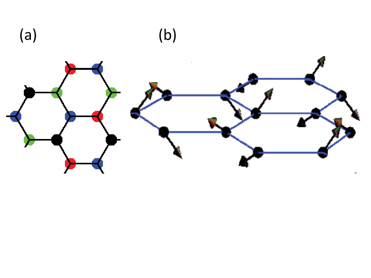
Since our result is at odd with that of Ref. [12] which applies in the limit of vanishing interaction strength, we further check the above conclusion by a variational Monte-Carlo (VMC) calculation using exactly the same parameters as for Figs.2. We adopted the partially-projected mean-field wave-functions[22] as our trial wave-functions, with the the form factors guided by the present SM-FRG result. Fig. 4 shows the energy gain per site due to pairing on (circles) and (triangles) lattices, showing negligible size dependence. We then compare to the energy gain associated with the chiral SDW (squares). It is clear that the SDW state is far more energetically favorable than the chiral -SC state at this doping level. The reason that the SDW state is realized in our lattice model lies in the fact that the perfect Fermi surface nesting is as important as the inter-saddle scattering addressed in Ref.[12].

Below 1/4 doping, the the Fermi level moves away from the van Hove points and the Fermi surface nesting worsens. This is shown in Fig. 5(a) for as an example. The bare interactions are still set as and . The SDW scattering is still attractive at high energies. As seen in Eq.(4), this relatively strong SDW channel causes attraction in the SC channel via overlap between these channels (terms with the projection operator in Eq. (4)). At even lower energy scales the pairing channel attraction (with ) continues to grow due to the Cooper instability, while the enhancement of the SDW scattering is saturated due to the lack of Fermi surface nesting. As the result the pairing instability surpasses the SDW instability at the lowest energy scale. This is shown by the flow of the singular values in Fig. 5(b). It is worth to mention that precisely the same phenomenon was observed in the FRG studies of the cuprates and pnictides[18, 15]. A close inspection of the eigenvectors associated with the most diverging superconducting pairing channel again find the degenerate and doublets, with dominant amplitudes for . The momentum space gap function of one of the pairing modes is shown in Fig. 5(a). Fig. 5(c) shows the renormalized for , which shows weak peaks at six independent and incommensurate momenta. Fig. 5(d) shows the renormalized for , which shows a strong negative peak at .

The above results imply degenerate -wave pairing instabilities. As for the degenerate SDW instabilities, additional analysis, such as the mean field theory or Ginzburg-Landau theory, is needed to fix the structure of the pairing function in the ordered state. To a large extent, this kind of analysis has been performed in Ref.[12]. We have also performed simple mean field calculations using the renormalized pairing interaction. The result is that a time-reversal breaking -wave pairing is always more favorable. This could have been anticipated since both and form factors have nodes on the Fermi surface, a natural way to gain energy is to form the above chiral d-wave pairing, which gaps out the entire Fermi surface.

We have also checked nearby doping and analyzed the competition between the incommensurate SDW and the SC state. In Fig. 6(a) we plot the higher diverging scale among these two competing orders as a function of doping (solid line). We found a similar phase diagram near -1/4 (hole) doping (not shown), mirroring that of electron doping. (Notice that the particle-hole symmetry is not exact in the presence of hopping integrals ).
We now discuss briefly the effect of the nearest neighbor interaction . As a typical example, we set and , and perform the FRG calculations. We find that the results are qualitatively similar to the cases with , except that in the leading pairing singular mode, becomes slightly stronger, but still smaller than by a factor of . The phase diagram for is also drawn in Fig.6(a) (dashed line). The critical scale is slightly higher than the case of . In the SC region this is due to the slight enhancement of -wave pairing on 2nd neighbor bonds. Unlike that claimed in Ref.[23], in all cases studied in this paper the -wave pairing is not a leading instability.
We end by presenting Fig. 6(b) as a schematic phase diagram in the temperature-doping plane. In reality when the doping level slightly deviates from 1/4, the extra charges will be localized by the presence of disorder, which enables the system to stay in the Chern insulator state for a finite doping interval. In the transition region marked by gray, where the doped charges delocalize, incommensurate SDW states with wave vectors shown in Fig.5(c) will emerge.
V Summary
In summary, we have performed SM-FRG calculations for parameters suitable for graphene. Our results indicate that near 1/4 electron- or hole- doping, graphene is either a Chern insulator or a chiral d-wave superconductors. Both phases are topological in nature, and deserve experimental efforts in searching them.
Acknowledgements.
We thank Hong Yao for helpful discussions, and are grateful to Tao Xiang for computing resources. QHW acknowledges the support by NSFC (under grant No.10974086 and 10734120) and the Ministry of Science and Technology of China (under grant No.2011CBA00108 and 2011CB922101). FY acknowledges the support by NSFC (under grant No.10704008). DHL acknowledges the support by the DOE grant number DE-AC02-05CH11231.VI Appendix
To illustrate the idea of the method, we first ignore the sublattice index, and return to it at a later stage.
The one-loop contributions to the flow of the irreducible 4-point vertex function is shown in Fig.7, where (a) and (b) lead to the flow of and , respectively, and (c)-(e) lead to the flow of . The internal Greens functions are convoluted with the form factors, hence
| (6) | |||||
where is the bare fermion propagator, is the area of the Brillouine zone. Here is the infrared cutoff of the Matsubara frequency .[24] As in usual FRG implementation, the self energy correction and frequency dependence of the vertex function are ignored.
In general, the form factor , where transforms according to an irreducible representation of the point group, and is the relative position vector between the two fermion fields on each side of the diagrams in Fig.1 (b)-(c). For two types of diagrams to overlap, all of the four fermion fields sit within the range set by the form factors. Hence the projections in Eq.(4) are all preformed in real space.

We now return to the honeycomb lattice with two sublattices. The necessary modifications are as follows: 1) The sublattice label can be absorbed into the labels in Figs.1, so in principle the label in the form factor also includes sublattice indices. However, once is fixed they are not independent. We absorb an independent index into the form factor label, , where labels fermion field 1 or 4 in Fig.1(b), 1 or 4 in (c), and 1 or 3 in (d). This is reasonable because the point group operations do not mix the sublattice when the center is chosen to be atomic sites. 2) In the presence of sublattice indices the Green’s functions are matrices. 3) In order to ensure that in momentum space , and transform exactly as product of form factors, care must be taken in choosing the phase of the Bloch states for complex unit cells.
The pairing function is determined as follows. A singular mode corresponds to a pairing operator in the momentum space, where is determined by (for all associated vectors ). The parity of the pairing matrix function under space inversion determines automatically whether it is a spin singlet or spin triplet. A further unitary transform can be used to get the momentum space gap function.

In the current implementation of SM-FRG the sampling of momentum space ( and ) is performed on self-adaptive meshes. As an example, Fig.8(a) shows the -mesh, which is progressively denser in approaching the Fermi surface or van Hove points (if they are close to the Fermi level). This is important for our problem because of the rapid variation of the Fermi velocity near the van Hove singularities. The -mesh is obtained as follows. First define an energy scale (of the order of the bandwidth), and begin with 6 equal-area triangles spanning the BZ. Break a specific triangle into four smaller equal-area ones if any eigen energy in the original triangle. Then lower the energy scale as () and repeat the above process recursively. The centers of the triangles form the mesh points. Combining the triangle areas, they are used in the loop integrations in Eq.(6). In our implementation, we perform the above processes 8-10 times, so that the last generation of triangles has a linear size of order , and the center of such triangles are sufficiently close to (or accidentally on) the Fermi surface. The -mesh as in Fig.8(b) used for the interactions includes all important scattering momenta: the origin and the high symmetry nesting vectors. We devise a function such that it is zero at those important scattering momenta, and generate the mesh in a similar fashion as for , except that becomes an artificial scale and is used in place of . Similar q-mesh already appears in Ref.[14].
References
- [1] K.S. Novoselov, A. K. Geim, S. V. Morozov, D. Jiang, Y. Zhang, S. V. Dubonos, I. V. Gregorieva, and A. A. Firsov, Science 306, 666 (2004).
- [2] For a review see A. H. Castro Neto, F. Guinea, N. M. R. Peres, K. S. Novoselov and A. K. Geim, Rev. Mod. Phys. 81, 109 (2009).
- [3] X. Du, I. Skachko, F. Duerr, A. Luican, and E. Y. Andrei, Nature 462, 192 (2009).
- [4] K. I. Bolotin, F. Ghahari, M. D. Shulman, H. L. Stormer, P. Kim, Nature 462, 196 (2009).
- [5] D. A. Siegel, Cheol-Hwan Park, C. Hwang, J. Deslippe, A. V. Fedorov, S. G. Louie, and A. Lanzara, PNAS 108, 11365 (2011); D. C. Elias, R. V. Gorbachev, A. s. Mayorov, S. V. Morozov, A. A. Zhukov, P. Blake, L. A. Ponomarenko, I. V. Grigorieva, K. S. Novoselov, F. Guinea, and A. K. Geim, Nature Phys. 7, 701 (2011).
- [6] A. L. Walter, A. Bostwick, K.-J. Jeon, F. Speck, M. Ostler, T. Seyller, L. Moreschini, Y. J. Chang, M. Polini, R. Asgari, A. H. MacDonald, K. Horn, and E. Rotenberg, Phys. Rev. B 84, 085410 (2011).
- [7] P. W. Anderson, Science 235, 1196 (1987).
- [8] S. Pathak, V. B. Shenoy, and G. Baskaran, Phys. Rev. B 81, 085431 (2010); arXiv:0809.0244.
- [9] A. M. Black-Schaffer, and S. Doniach, Phys. Rev. B 75, 134512 (2007).
- [10] J. González, Phys. Rev. B 78, 205431 (2008); C. A. Lamas, D. C. Cabra, and N. Grandi, Phys. Rev. B 80, 075108 (2009); D. Makogon, R. van Gelderen, R. Roldán, and C. M. Smith, Phys. Rev. B 84, 125404 (2011).
- [11] E. V. Castro, A. G. Grushin, B. Valenzuela, M. A. H. Vozmediano, A. Cortijo, and F. de Juan, Phys. Rev. Lett. 107, 106402 (2011).
- [12] R. Nandkishore, L. Levitov, and A. Chubukov, arXiv:1107.1903.
- [13] Tao Li, arXiv:1103.2420.
- [14] C. Husemann, and M. Salmhofer, Phys. Rev. B 79, 195125 (2009).
- [15] H. Zhai, F. Wang, and D.-H. Lee, Phys. Rev. B 80, 064517 (2009).
- [16] C. Honerkamp, Phys. Rev. Lett. 100, 146404 (2008).
- [17] M. Salmhofer and C. Honerkamp, Prog. Theor. Phys. 105, 1 (2001).
- [18] C. Honerkamp, M. Salmhofer, N. Furukawa, and T. M. Rice, Phys. Rev. B 63, 035109 (2001).
- [19] F. Wang, H. Zhai, Y. Ran, A. Vishwanath, and D.-H. Lee, Phys. Rev. Lett. 102, 047005 (2009).
- [20] We note by setting above does not produce independent spatial form factors because the above three form factors are complete for the three 1st neighbor bonds. Hence by using we are able to investigate, e.g., both - and -wave pairing (of course their total form factors have completely different spin and sublattice structures).
- [21] Translating , and back to , the divergence criterion is smaller since two form factors must be accounted for.
- [22] Fan Yang, Hui Zhai, Fa Wang, Dung-Hai Lee, Phys. Rev. B 83, 134502 (2011)
- [23] M. Kiesel, C. Platt, W. Hanke, D. A. Abanin, R. Thomale, arXiv:1109.2953. In this paper the electron filling is defined as the number of electrons per site per spin, which is related to our doping level as .
- [24] C. Karrasch, R. Hedden, R. Peters, Th. Pruschke, K. Schönhammer, and V. Meden, J. Phys. Cond. Matt. 20, 345205 (2008).