1Introduction

\TheoremsNumberedThrough\ECRepeatTheorems\EquationsNumberedThrough\MANUSCRIPTNO

\RUNAUTHOR

Su and El Gamal

\RUNTITLE

Limits on the Benefits of Energy Storage for Renewable Integration

\TITLE

Limits on the Benefits of Energy Storage for Renewable Integration

\ARTICLEAUTHORS\AUTHOR

Han-I Su \AFFDepartment of Electrical Engineering, Stanford University, Stanford, CA 94305, \EMAILhanisu@stanford.edu \AUTHORAbbas El Gamal \AFFDepartment of Electrical Engineering, Stanford University, Stanford, CA 94305, \EMAILabbas@ee.stanford.edu

\ABSTRACT

The high variability of renewable energy resources presents significant challenges to the operation of the electric power grid. Conventional generators can be used to mitigate this variability but are costly to operate and produce carbon emissions. Energy storage provides a more environmentally friendly alternative, but is costly to deploy in large amounts. This paper studies the limits on the benefits of energy storage to renewable energy: How effective is storage at mitigating the adverse effects of renewable energy variability? How much storage is needed? What are the optimal control policies for operating storage? To provide answers to these questions, we first formulate the power flow in a single-bus power system with storage as an infinite horizon stochastic program. We find the optimal policies for arbitrary net renewable generation process when the cost function is the average conventional generation (environmental cost) and when it is the average loss of load probability (reliability cost). We obtain more refined results by considering the multi-timescale operation of the power system. We view the power flow in each timescale as the superposition of a predicted (deterministic) component and an prediction error (residual) component and formulate the residual power flow problem as an infinite horizon dynamic program. Assuming that the net generation prediction error is an IID process, we quantify the asymptotic benefits of storage. With the additional assumption of Laplace distributed prediction error, we obtain closed form expressions for the stationary distribution of storage and conventional generation. Finally, we propose a two-threshold policy that trades off conventional generation saving with loss of load probability. We illustrate our results and corroborate the IID and Laplace assumptions numerically using datasets from CAISO and NREL.

\KEYWORDS

energy storage, renewable integration, dynamic programming

1 Introduction

The rapid increase in the world demand for electricity (EIA 2011, Figure 72) coupled with the need to reduce the high carbon emissions due to electric power generation from fossil fuel (EPA 2011, Table 3-7) are driving a dramatic increase in renewable energy generation from sources such as wind, solar, and hydro. The power generated from wind and solar, however, is intermittent and uncertain, which presents significant challenges to power system operation as the penetration of these sources increases (NREL 2010). In the long timescale (weeks to hours), this variability causes power imbalances: When renewable generation falls short of meeting the demand, more conventional generation from combined-cycle combustion and gas turbines is needed, which increases power system operation cost and offsets some of the environmental benefits of renewable energy (Hart and Jacobson 2011); when renewable generation exceeds demand, the excess power generated must be curtailed. In the short timescale (minutes to seconds), the variability of renewable generation can lead to large frequency and voltage variations and higher loss of load probability.

In addition to using conventional generation, renewable energy variability can be mitigated architecturally via geographical generation diversity (NREL 2010) and renewable resource diversity (Li et al. 2009), and operationally using demand-response (Kirby and Milligan 2010) and energy storage (Denholm et al. 2010, Bitar et al. 2011). In particular, energy storage can help in two quite different ways (EPRI 2010).

•

In the long timescale, bulk energy storage systems, such as pumped hydroelectric storage and compressed air energy storage (CAES), can be charged by the excess renewable energy generation during off-peak hours and discharged during peak hours, hence reducing the need for additional conventional generation capacity, and renewable energy curtailment.
•

In the short timescale, fast-response energy storage systems, such as flywheels and batteries, can also help improve reliability beyond what fast-ramping generation can achieve because of their much faster response time.

This paper aims to establish the limits on the benefits of storage for mitigating renewable energy variability. How much can storage help reduce the need for conventional generation? How much can it help improve reliability? How much storage is needed to reap these benefits? What are the optimal control policies that achieve these limits? Satisfactory answers to these questions can help in architecting the smart grid as well as in operating it efficiently and reliably. Since we wish to establish limits on the benefits of storage rather than analyzing the operation of a particular power system with storage, we will ignore the fixed and operating costs of storage as well as explicit economic benefits such as arbitrage (e.g. see Eyer and Corey (2010)) throughout this paper. Under certain assumptions, we will find that most of the benefits can be achieved with only a modest amount of storage.

Following is an outline of the rest of the paper:

•

In Section 2, we consider a single-bus power system with storage and a slotted-time model for load and energy generation. We formulate the power flow problem as an infinite horizon average-cost stochastic program in which the input is the net renewable generation (difference between the renewable power generated and the demand) and the controls are conventional generation and the storage charging and discharging operations. We consider two cost functions, the expected average conventional generation (environmental cost) and the expected average loss of load probability (reliability cost). We find the optimal policies for each of these cost functions for arbitrary net renewable generation process (Theorems 2.1 and 2.4). The performance of these policies is illustrated using load data from CAISO (2012) and simulated renewable wind power generation data from NREL (Potter et al. 2008).
•

In Section 3, we make progress toward quantifying the degree to which storage can help mitigate the impacts of renewable generation and the amount of storage needed. We consider the multi-timescale operation of the power system (day-ahead, hour-ahead, minutes-ahead, and real time). For each timescale, we view power flow in the single-bus power system with storage as the superposition of a predicted (deterministic) component and an error (residual) random component. We assume that the predicted component is balanced (with possibly a fixed offset) and formulate the residual power flow problem as an infinite horizon average-cost dynamic program with the net renewable generation prediction error as input and fast-ramping generation and storage as control variables. Assuming that the net renewable generation error is an IID process, we show that storage can reduce fast-ramping generation (relative to no storage) by a factor that approaches the storage round-trip inefficiency as its capacity becomes large (Proposition 3.1). We further show that storage can reduce the average loss of load probability to zero as storage capacity becomes large (Proposition 3.4).

We then observe from the NREL simulated wind power dataset that in the short timescale (minutes), the wind power generation prediction error is close to Laplace distributed. Under this additional assumption, we obtain closed form expressions for the minimum average fast-ramping generation and the stationary distribution of the stored power sequence in some special cases (Propositions 3.2 and 3.3). We show that most of the possible reduction in conventional generation can be achieved with relatively small storage capacity. We also show that the average loss of load probability can be reduced by an order of magnitude with small storage capacity.
•

The optimal policies we establish in Section 2 represent two extremes: The policy that minimizes the average conventional generation always uses the stored energy ahead of conventional generation and never uses conventional generation to charge storage, while the policy that minimizes the average loss of load probability uses conventional generation ahead of stored energy and to keep storage as full as possible. In Section 4, we present a two-threshold policy that includes these two policies as special cases. We also show that this policy minimizes the one-period weighted sum of the aforementioned cost functions and is optimal for all the numerical examples we tried. Using this policy, we find a tradeoff between conventional generation capacity and storage capacity needed to achieve prescribed conventional generation consumption and loss of load probability.
•

In Section 5 we generalize the policies established in Section 2 to the case where the storage charging and discharging rates are constrained (Theorems 5.1 and 5.2). We find that most of the benefit to average conventional generation can be attained with relatively small charging and discharging rates, while higher such rates are needed for the average loss of load probability.

This paper is a significantly reorganized and expanded version of the conference paper (Su and Gamal 2011). There is a large body of previous work on energy storage. An overview of energy storage technologies and applications can be found in EPRI (2010), Roberts and Sandberg (2011) and references therein. Prior related work to this paper include Chandy et al. (2010), Gayme and Topcu (2011), Oh (2011). Both Chandy et al. (2010) and Gayme and Topcu (2011) assume that the net load is deterministic. Chandy et al. (2010) formulate a dynamic dc optimal power flow problem with energy storage as a convex program. The optimal policy is established explicitly for some special cases. Gayme and Topcu (2011) formulate a dynamic ac optimal power flow problem with energy storage. The problem is shown to be non-convex in general, and sufficient conditions for strong duality are established. Oh (2011) models renewable generation as a sequence of discrete random variables. An approximate stochastic programming method is proposed and illustrated via numerical examples. Concurrent and independent related work to this paper include Koutsopoulos et al. (2011) and ParandehGheibi et al. (2011) in which continuous-time models for the net renewable generation are considered with different problem formulations.

2 Single-bus power system with storage

Consider the single-bus electric power system with storage depicted in Figure 2, which consists of conventional generation, net renewable generation (difference between the renewable generation and the load), and energy storage. This power system may represent a transmission network with high renewable penetration, a distribution network with distributed renewable generators and energy storage devices, a microgrid not operated in the island mode where the power from the macrogrid acts as a fast-ramping generator (Lasseter et al. 2002), a wind farm with energy storage devices in which generation is acquired through an electricity market, or a stand-alone hybrid renewable energy system with battery storage (Deshmukh and Deshmukh 2008, Bernal-Agustín and Dufo-López 2009). The conventional generation may include base-load generators (coal-fired, hydro, and nuclear power plants), intermediate generators (combined-cycle combustion turbine), and peaking and fast-ramping generators (gas turbines). The renewable generation may include wind and solar. The numerical results in this paper assume only wind power. The energy storage may include bulk energy storage (compressed air and pumped hydroelectric storage) and fast-response energy storage (flywheels and batteries).

\FIGURE

Single-bus power system with storage.

We assume a slotted-time model for the dynamics of the power system, where time is divided into slots each of length $\tau$ hours and power is constant over each time slot. In the following, we introduce the needed definitions and the assumptions used throughout the paper.

•

The power supplied by the net renewable generation (difference between the renewable generation power and the load) in time slot $i=1,2,\ldots$ is denoted by $\Delta_{i}$ . The sequence $\Delta_{1},\Delta_{2},\ldots$ is in general a random process.
•

We denote the total power capacity of conventional generation by $G_{\mathrm{max}}$ MW. The power supplied in time slot $i=1,2,\ldots$ is denoted by $G_{i}\leq G_{\mathrm{max}}$ .

We characterized energy storage by the following parameters:

•

The energy storage capacity $\tau S_{\mathrm{max}}$ MW-h is the maximum amount of energy that can be stored, where $S_{\mathrm{max}}$ is referred to as the power storage capacity. Real-world energy storage devices cannot be completely discharged, and there is a limit on their minimum energy level. We use this minimum level as a reference and assume without loss of generality that it is equal to zero.
•

The stored power at the beginning of time slot $i=1,2,\ldots$ is denoted by $S_{i}$ MW.
•

The rated storage power conversion $C_{\mathrm{max}}$ MW is the maximum input (charging) power. The charging power at time $i=1,2,\ldots$ is denoted by $C_{i}\leq C_{\mathrm{max}}$ .
•

The rated storage output power $D_{\mathrm{max}}$ MW is the maximum output (discharging) power. The discharging power at time $i=1,2,\ldots$ is denoted by $D_{i}\leq D_{\mathrm{max}}$ .
•

The charging efficiency $\alpha_{\mathrm{c}}\in(0,1)$ is the ratio of the charged power to the input power. The discharging efficiency $\alpha_{\mathrm{d}}\in(0,1)$ is the ratio of the output power to the discharged power. The round-trip efficiency therefore is $\alpha=\alpha_{\mathrm{c}}\alpha_{\mathrm{d}}$ .
•

The storage efficiency is the fraction of retained power over a time slot. We assume throughout that the storage efficiency is very high compared to the round-trip efficiency and assume that it is equal to one.

Using the above definitions, we can express the dynamics of the stored energy as

\displaystyle S_{i+1}

\displaystyle=S_{i}+\alpha_{\mathrm{c}}C_{i}-\frac{1}{\alpha_{\mathrm{d}}}D_{i}\quad\text{for}\ i=1,2,\ldots

with the constraints $0\leq S_{i}\leq S_{\mathrm{max}}$ , $0\leq C_{i}\leq C_{\mathrm{max}}$ , and $0\leq D_{i}\leq D_{\mathrm{max}}$ , where $S_{1}\in[0,S_{\mathrm{max}}]$ is given.

In Sections 2 through 4, we will assume unconstrained rated output power and power conversion of the energy storage, i.e.,

\displaystyle\alpha_{\mathrm{c}}C_{\mathrm{max}}

\displaystyle=\frac{1}{\alpha_{\mathrm{d}}}D_{\mathrm{max}}=S_{\mathrm{max}}.

(1)

The general case is discussed in Section 5.

We assume that the (negative) net renewable generation power is to be balanced as much as possible by conventional generation and stored power:

•

If $\Delta_{i}\geq-G_{\mathrm{max}}-\min\{\alpha_{\mathrm{d}}S_{i},D_{\mathrm{max}}\}$ , then there is sufficient power capacity and the balance constraint must be satisfied, i.e., $G_{i}+D_{i}-C_{i}+\Delta_{i}\geq 0$ . Note that if $G_{i}+D_{i}-C_{i}+\Delta_{i}>0$ , then there is excess generation. We assume that this excess generation is curtailed.
•

If $\Delta_{i}<-G_{\mathrm{max}}-\min\{\alpha_{\mathrm{d}}S_{i},D_{\mathrm{max}}\}$ , then loss of load occurs. In this case, conventional generation is at its power capacity and storage is discharged at the rated storage output power, i.e., $G_{i}=G_{\mathrm{max}}$ , $C_{i}=0$ , and $D_{i}=\min\{\alpha_{\mathrm{d}}S_{i},D_{\mathrm{max}}\}$ .

In the following two subsections, we formulate the power flow problem in the single-bus system as infinite horizon stochastic programs with two different cost functions. We establish the optimal control policies for both cost functions for arbitrary net renewable generation process. In Subsection 2.3, we illustrate these policies using datasets from CAISO and NREL.

2.1 Minimizing average conventional generation

The first cost function we consider is the expected long term average conventional generation. This is motivated by the need to reduce the carbon emissions of conventional generation. We seek to minimize this cost function by controlling the amount of conventional generation $G_{i}$ , charging $C_{i}$ , and discharging $D_{i}$ used in each time slot $i=1,2,\ldots$ , where the triple $(G_{i},C_{i},D_{i})$ is a function of the history $H_{i}=(S_{1},\Delta_{1},S_{2},\Delta_{2},\ldots,S_{i-1},\Delta_{i-1},S_{i})$ . A control policy $\pi$ is a sequence of these triples, i.e., $\pi=\{(G_{i},C_{i},D_{i}):\,i=1,2,\ldots\}$ . A policy is said to be stationary if $\pi_{i}=\pi_{j}$ for all $i$ and $j$ . We are now ready to define the first optimization problem.

Stochastic program I: Minimizing average conventional generation.

	minimize	$\displaystyle{\cal J}^{(1)}(\pi,S_{1})=\limsup_{n\to\infty}\E\left[\frac{1}{n}\sum_{i=1}^{n}G_{i}\right]$
	subject to	$\displaystyle S_{i+1}=S_{i}+\alpha_{\mathrm{c}}C_{i}-\frac{1}{\alpha_{\mathrm{d}}}D_{i},$
		$\displaystyle 0\leq S_{i}\leq S_{\mathrm{max}},\qquad\ 0\leq C_{i},$
		$\displaystyle 0\leq G_{i}\leq G_{\mathrm{max}},\qquad 0\leq D_{i},$
		$\displaystyle 0\leq G_{i}-C_{i}+D_{i}+\max\{\Delta_{i},-G_{\mathrm{max}}-\alpha_{\mathrm{d}}S_{i}\},$

where the expectation is over the net renewable generation sequence $\Delta_{i}$ , $i=1,2,\ldots$ . We denote the optimal policy by $\pi^{(1)}$ .

It turns out that a simple stationary policy is optimal for arbitrary net renewable generation process (including deterministic sequences).

Theorem 2.1

The optimal policy $\pi^{(1)}$ for stochastic program I is given in Table 2.1.

The optimal policy is illustrated by the “phase-diagram” in Figure 2.1. When the prediction error $\delta\geq 0$ , the optimal policy charges the storage using the excess renewable generation as much as possible. When the prediction error $\delta<0$ , the storage is first discharged to compensate for as much of the renewable power deficit as possible. Conventional generation is then used to compensate for the remaining renewable generation deficit (if any). Thus, the optimal policy $\pi^{(1)}$ never charges the storage using conventional generation. This greedy policy is a consequence of the linearity of the cost function and the imperfect round-trip storage efficiency as will become clear in the proof.

\TABLE

Optimal policy in Theorem 2.1 and corresponding stored power dynamics. $\pi^{(1)}_{i}$ $G^{(1)}_{i}$ $C^{(1)}_{i}$ $D^{(1)}_{i}$ $S_{i+1}$ $\displaystyle\frac{S_{\mathrm{max}}-S_{i}}{\alpha_{\mathrm{c}}}\leq\Delta_{i}$ $0$ $\displaystyle\frac{S_{\mathrm{max}}-S_{i}}{\alpha_{\mathrm{c}}}$ $0$ $S_{\mathrm{max}}$ $\displaystyle 0\leq\Delta_{i}<\frac{S_{\mathrm{max}}-S_{i}}{\alpha_{\mathrm{c}}}$ $0$ $\Delta_{i}$ $0$ $S_{i}+\alpha_{\mathrm{c}}\Delta_{i}$ $-\alpha_{\mathrm{d}}S_{i}\leq\Delta_{i}<0$ $0$ $0$ $-\Delta_{i}$ $S_{i}+\Delta_{i}/\alpha_{\mathrm{d}}$ $-G_{\mathrm{max}}-\alpha_{\mathrm{d}}S_{i}\leq\Delta_{i}<-\alpha_{\mathrm{d}}s_{i}$ $-\Delta_{i}-\alpha_{\mathrm{d}}S_{i}$ $0$ $\alpha_{\mathrm{d}}S_{i}$ $0$ $\Delta_{i}<-G_{\mathrm{max}}-\alpha_{\mathrm{d}}S_{i}$ $G_{\mathrm{max}}$ $0$ $\alpha_{\mathrm{d}}S_{i}$ $0$

\FIGURE

Illustration of the optimal policy $\pi^{(1)}$ in Theorem 2.1. The value in each region corresponds to the stored power at the end of slot $i$ when the stored power and prediction error at the beginning of this slot are $S_{i}$ and $\Delta_{i}$ , respectively.

To prove the theorem, consider the finite horizon counterpart of stochastic program I. Define the cost-to-go function

\displaystyle J^{(1)}_{k}(\pi,H_{k})=\E\left[\left.\sum_{i=k}^{n}G_{i}\right|H_{k}\right].

Let $\pi^{*}$ be the policy achieving $\inf_{\pi}J^{(1)}_{k}(\pi,H_{k})$ . For a fixed pair $(H_{k-1},\Delta_{k-1})$ , we will use the shorter notation $J^{(1)}_{k}(\pi^{*},S_{k})$ in place of $J^{(1)}_{k}(\pi^{*},H_{k-1},\Delta_{k-1},S_{k})$ . In the following lemma, we establish key properties of the cost-to-go function. The rest of the proof of Theorem 2.1 is given in Appendix 7.

Lemma 2.2

The minimum cost-to-go function must satisfy the conditions:

1.

$J^{(1)}_{k}(\pi^{*},S_{k}+c)\leq J^{(1)}_{k}(\pi^{*},S_{k})$ for $0\leq c\leq S_{\mathrm{max}}-S_{k}$ , i.e., excess energy is not curtailed until storage is fully charged..
2.

$J^{(1)}_{k}(\pi^{*},S_{k}+c)\geq J^{(1)}_{k}(\pi^{*},S_{k})-\alpha_{\mathrm{d}}c$ for $0\leq c\leq S_{\mathrm{max}}-S_{k}$ , i.e., the cost of using conventional generation to charge storage by $c$ MW is $c/\alpha_{\mathrm{c}}$ , but the reduction in cost is at most $\alpha_{\mathrm{d}}c$ .

Proof 2.3

To prove part 1, given the optimal policy $\pi^{*}$ , we find another policy $\pi$ such that $J^{(1)}_{k}(\pi,S_{k}+c)=J^{(1)}_{k}(\pi^{*},S_{k})$ . Let $H_{i}$ and $H_{i}^{*}$ be the history sequences under the policy $\pi$ and $\pi^{*}$ , respectively. For fixed $(H_{k-1},\Delta_{k-1})$ , consider $H_{k}=(H_{k-1},\Delta_{k},S_{k}+c)$ and $H_{k}^{*}=(H_{k-1},\Delta_{k},S_{k})$ . Let

\displaystyle G_{i}

\displaystyle=G_{i}^{*},\qquad D_{i}=D_{i}^{*},\qquad C_{i}=\min\left\{C_{i}^{*},\frac{1}{\alpha_{\mathrm{c}}}\left(S_{\mathrm{max}}-S_{i}+\frac{1}{\alpha_{\mathrm{d}}}D_{i}^{*}\right)\right\}.

(2)

The policy $\pi$ is illustrated in Figure 2.1. By induction, the stored power under policy $\pi$ is always higher than that under policy $\pi^{*}$ . Thus, by definition, $J^{(1)}_{k}(\pi^{*},S_{k})=J^{(1)}_{k}(\pi,S_{k}+c)\geq J^{(1)}_{k}(\pi^{*},S_{k}+c).$

To prove part 2 of the lemma, given the optimal policy $\pi^{*}$ , we find a policy $\pi$ such that $J^{(1)}_{k}(\pi,S_{k})\leq J^{(1)}_{k}(\pi^{*},S_{k}+c)+\alpha_{\mathrm{d}}c$ . For fixed $(H_{k-1},\Delta_{k-1})$ , consider $H_{k}=(H_{k-1},\Delta_{k},S_{k})$ and $H_{k}^{*}=(H_{k-1},\Delta_{k},S_{k}+c)$ . Let

\displaystyle C_{i}

\displaystyle=C_{i}^{*},\qquad D_{i}=\min\{D_{i}^{*},\alpha_{\mathrm{d}}(S_{i}+\alpha_{\mathrm{c}}C_{i}^{*})\},\qquad G_{i}=\min\{G_{i}^{*}+D_{i}^{*}-D_{i},G_{\mathrm{max}}\}.

(3)

The policy $\pi$ is illustrated in Figure 2.1. By induction, the stored power under policy $\pi$ is always lower than the stored power under policy $\pi^{*}$ . The cost-to-go function of policy $\pi$ can be upper bounded as

	$\displaystyle J^{(1)}_{k}(\pi,S_{k})$	$\displaystyle\leq\E\left[\left.\sum_{i=k}^{n}G_{i}^{}+\alpha_{\mathrm{d}}((S_{i}^{}-S_{i})-(S_{i+1}^{*}-S_{i+1}))\right\|H_{k}\right]$
		$\displaystyle=J^{(1)}_{k}(\pi^{},S_{k}+c)+\alpha_{\mathrm{d}}\E\left[\left.(S_{k}^{}-S_{k})-(S_{n+1}^{*}-S_{n+1})\right\|H_{k}\right]$
		$\displaystyle\leq J^{(1)}_{k}(\pi^{*},S_{k}+c)+\alpha_{\mathrm{d}}c.$

\FIGURE

(a) Part 1

(b) Part 2

Illustration for the proof of Lemma 2.2.

2.2 Minimizing average loss of load probability

As we mentioned, energy storage can be used to improve power system reliability in the presence of renewable energy variation. As a measure of system reliability, we use the average loss of load probability. Define the loss of load cost at time $i$ as

\displaystyle 1_{\{\Delta_{i}<-G_{\mathrm{max}}-\min\{\alpha_{\mathrm{d}}S_{i},D_{\mathrm{max}}\}\}}=\begin{cases}1&\text{if }\Delta_{i}<-G_{\mathrm{max}}-\min\{\alpha_{\mathrm{d}}S_{i},D_{\mathrm{max}}\}\\ 0&\text{otherwise.}\end{cases}

(4)

We wish to find the control policy $\pi=\{(G_{i},C_{i},D_{i}):\,i=1,2,\ldots\}$ that minimizes the expected average loss of load cost.

Stochastic program II: Minimizing average loss of load.

	minimize	$\displaystyle{\cal J}^{(2)}(\pi,S_{1})=\limsup_{n\to\infty}\E\left[\frac{1}{n}\sum_{i=1}^{n}1_{\{\Delta_{i}<-G_{\mathrm{max}}-\alpha_{\mathrm{d}}S_{i}\}}\right]$
	subject to	$\displaystyle S_{i+1}=S_{i}+\alpha_{\mathrm{c}}C_{i}-\frac{1}{\alpha_{\mathrm{d}}}D_{i},$
		$\displaystyle 0\leq S_{i}\leq S_{\mathrm{max}},\qquad\ 0\leq C_{i},$
		$\displaystyle 0\leq G_{i}\leq G_{\mathrm{max}},\qquad 0\leq D_{i},$
		$\displaystyle 0\leq G_{i}-C_{i}+D_{i}+\max\{\Delta_{i},-G_{\mathrm{max}}-\alpha_{\mathrm{d}}S_{i}\},$

where the expectation is over the net renewable generation sequence $\Delta_{i}$ , $i=1,2,\ldots$ . We denote the optimal policy by $\pi^{(2)}$ .

The optimal policy for this program is simply to keep the stored power as high as possible by using both excess renewable and conventional generation. The policy again holds for an arbitrary net renewable generation process.

Theorem 2.4

The optimal policy $\pi^{(2)}$ for stochastic program II is given in Table 2.2.

\TABLE

Optimal policy in Theorem 2.4 and corresponding stored power. $\pi^{(2)}_{i}$ $G^{(2)}_{i}$ $C^{(2)}_{i}$ $D^{(2)}_{i}$ $S_{i+1}$ $\displaystyle\frac{S_{\mathrm{max}}-S_{i}}{\alpha_{\mathrm{c}}}\leq\Delta_{i}$ $0$ $\displaystyle\frac{S_{\mathrm{max}}-S_{i}}{\alpha_{\mathrm{c}}}$ $0$ $S_{\mathrm{max}}$ $\displaystyle-G_{\mathrm{max}}+\frac{S_{\mathrm{max}}-S_{i}}{\alpha_{\mathrm{c}}}\leq\Delta_{i}<\frac{S_{\mathrm{max}}-S_{i}}{\alpha_{\mathrm{c}}}$ $\displaystyle\frac{S_{\mathrm{max}}-S_{i}}{\alpha_{\mathrm{c}}}-\Delta_{i}$ $\displaystyle\frac{S_{\mathrm{max}}-S_{i}}{\alpha_{\mathrm{c}}}$ $0$ $S_{\mathrm{max}}$ $\displaystyle-G_{\mathrm{max}}\leq\Delta_{i}<-G_{\mathrm{max}}+\frac{S_{\mathrm{max}}-S_{i}}{\alpha_{\mathrm{c}}}$ $G_{\mathrm{max}}$ $G_{\mathrm{max}}+\Delta_{i}$ $0$ $S_{i}+\alpha_{\mathrm{c}}(G_{\mathrm{max}}+\Delta_{i})$ $\displaystyle-G_{\mathrm{max}}-\alpha_{\mathrm{d}}S_{i}\leq\Delta_{i}<-G_{\mathrm{max}}$ $G_{\mathrm{max}}$ $0$ $-\Delta_{i}-G_{\mathrm{max}}$ $\displaystyle S_{i}+\frac{G_{\mathrm{max}}+\Delta_{i}}{\alpha_{\mathrm{d}}}$ $\Delta_{i}<-G_{\mathrm{max}}-\alpha_{\mathrm{d}}S_{i}$ $G_{\mathrm{max}}$ $0$ $\alpha_{\mathrm{d}}S_{i}$ $0$

Since there is no conventional generation cost, in some cases the optimal policy charges the storage with conventional generation to minimize the loss of load probability as illustrated in the phase-diagram in Figure 2.2,.

\FIGURE

Illustration of the optimal policy in Theorem 2.4.

To prove the theorem, we again consider its finite horizon counterpart and define the cost-to-go function as

\displaystyle J^{(2)}_{k}(\pi,H_{k})=\E\left[\left.\sum_{i=k}^{n}1_{\{\Delta_{i}<-G_{\mathrm{max}}-\alpha_{\mathrm{d}}S_{i}\}}\right|H_{k}\right].

Let $\pi^{*}$ be the policy achieving $\inf_{\pi}J^{(2)}_{k}(\pi,H_{k})$ . For a fixed pair $(H_{k-1},\Delta_{k-1})$ , we will used the shorter notation $J^{(2)}_{k}(\pi,S_{k})$ in place of $J^{(2)}_{k}(\pi,H_{k-1},\Delta_{k-1},S_{k})$ . The key step in the proof is to show

\displaystyle J^{(2)}_{k}(\pi^{*},S_{k}+c)\leq J^{(2)}_{k}(\pi^{*},S_{k})\quad\text{for}\ 0\leq c\leq S_{\mathrm{max}}-S_{k}.

(5)

This follows since the policy $\pi$ defined in (2) always has higher stored power than the optimal policy $\pi^{*}$ . Since the loss of load probability cannot increase if the amount of stored power is increased, we have $J^{(2)}_{k}(\pi^{*},S_{k})\geq J^{(2)}_{k}(\pi,S_{k}+c)\geq J^{(2)}_{k}(\pi^{*},S_{k}+c).$ The rest of the proof of Theorem 2.4 is given in Appendix 7.

2.3 Numerical results

To investigate the reduction in conventional generation and loss of load probability attained by using energy storage, we use the simulated Western Wind Dataset from NREL (Potter et al. 2008) and the actual load dataset from CAISO (2012). The NREL dataset is based on numerical weather prediction (NWP) models. It attempts to recreate the potential wind power generation of more than 30 000 sites with ten 3 MW turbines at each location in the western U.S from 2004 to 2006, and the wind power data is sampled every 10 minutes. The CAISO load dataset includes the hourly load in California in 2004. Figure 2.3 plots the total simulated hourly power output of the wind turbines and the hourly load in California.

Figure 2.3 shows the average conventional generation under the optimal policy $\pi^{(1)}$ for several values of power storage capacities and round-trip storage efficiencies $\alpha=60\%$ and $80\%$ . As can be seen from the figure, conventional generation consumption can be reduced using storage by $44\%$ and $53\%$ for $\alpha=60\%$ and $80\%$ , respectively, when the storage capacity is 60 times the total rated power of the wind turbines, which is equivalent to 914 GW-h of storage. Note that $80\%$ of this reduction can be achieved by power storage capacity equal to 15 times the total rated power of the wind turbines, i.e., 228 GW-h.

Figure 2.3 plots the average loss of load probability under the optimal policy $\pi^{(2)}$ for several values of power storage capacities and round-trip storage efficiencies $\alpha=60\%$ and $80\%$ . For large $S_{\mathrm{max}}$ , the reduction in the loss of load probability is roughly exponential in $S_{\mathrm{max}}$ . We also see that the average loss of load probability can be reduced by an order of magnitude with power storage capacity less than 2 standard deviations of the net renewable generation process.

3 Residual power system

In the previous section, we formulated the single-bus power system stochastic programs I and II and found the optimal policies $\pi^{(1)}$ and $\pi^{(2)}$ that minimize expected average conventional generation and average loss of load probability, respectively, for arbitrary net renewable generation process. These policies provide answers to the question concerning optimal storage control policies. Although answers to the other questions we seek to answer can be obtained numerically as illustrated in Subsection 2.3, the results lump together vastly different types of conventional generation and storage resources that are deployed at very different timescales. Electric power systems are typically operated in multiple timescales as illustrated in Figure 3:

•

Day-ahead: Each day, an hourly prediction of the net load (the negative of the net renewable generation) for the next day is made. Base generation and bulk storage are scheduled to meet this prediction.
•

Hour-ahead: Each hour, a refined prediction of the net load in the next hour is made. Peaking generation and medium-response storage are scheduled to meet the difference (prediction error) between the day-ahead and hour-ahead prediction.
•

Minutes-ahead: Every few minutes, a prediction of the net load in the next few minutes is made. Fast-ramping generation and fast-response storage are scheduled to balance the difference between the minutes-ahead and hour-ahead prediction.
•

Real-time: The scheduled generation and storage are operated. The deviation of actual net load from the minutes-ahead prediction is matched by additional fast-ramping generation and fast-response storage.

\FIGURE

Multi-timescale power grid operation.

Consider the multi-timescale power system operation. The day-ahead power flow prediction can be modeled in the same manner as the single-bus power system discussed in the previous section. In each subsequent timescale, the system can be decomposed into a scheduled (deterministic) part and a residual (random) part as depicted in Figure 3. We assume that the scheduled generation and storage power balance the predicted net renewable generation power; hence we can model the residual power system in exactly the same manner as the original system studied in Section 2, except that the input is now the net renewable generation prediction error and the controls are fast-ramping generation and the charging and discharging of the fast-response energy storage. Unlike net renewable generation, which is in general a messy stochastic process, under good prediction, the prediction error process can be modeled as an IID zero-mean process $\Delta_{i}$ , $i=1,2,\ldots$ , with variance $\Var[\Delta_{i}]=\sigma^{2}$ (see Subsection 3.4 for numerical justification of this assumption). In Subsection 3.3, we consider the case of over provisioning in which more power is scheduled than the predicted net renewable generation, that is, the mean of the prediction error $\E[\Delta_{i}]>0$ .

\FIGURE

Decomposition of the total single-bus power system into a scheduled (predicted) power component and a residual power system component.

3.1 Minimizing average fast-ramping generation

We first consider the role of fast-response energy storage in reducing the required fast-ramping generation. The formulation of this problem is the same as stochastic program I, but with the additional assumption that $\Delta_{i}$ , $i=1,2,\ldots$ , is an IID process with zero-mean and variance $\Var[\Delta_{i}]=\sigma^{2}$ . We refer to this new problem as dynamic program I. Since the optimal policy $\pi^{(1)}$ in Theorem 2.1 for stochastic program I holds for any net renewable generation process, it is optimal for dynamic program I. The IID assumption, however, allows us to provide some answers to the question of how much storage can help.

Consider the extreme case in which the fast-ramping generation capacity $G_{\mathrm{max}}$ is unlimited. If there is no storage, i.e., $S_{\mathrm{max}}=0$ , then it is not difficult to see that the average cost is $\E[\Delta^{-}]$ , where $x^{-}=\max\{-x,0\}$ . The minimum expected average fast-ramping generation for unlimited storage is given in the following.

Proposition 3.1

For unlimited $G_{\mathrm{max}}$ and $S_{\mathrm{max}}$ , the minimum average cost is ${\cal J}^{(1)}(\pi^{(1)},S_{1})=(1-\alpha)\E[\Delta^{-}]$ .

The proof of this proposition is given in Appendix 8.

Comparing the average costs for no storage to unlimited power storage capacity, this proposition shows that storage can reduce the amount of needed fast-ramping generation (relative to no storage) in the limit by a factor equal to the round-trip storage inefficiency. This is not surprising because the IID zero-mean prediction error assumption implies that over the long term, the excess energy is roughly equal to the deficit. With infinite capacity and $\alpha=1$ , storage can compensate for almost all the variation in renewable generation. However, when $\alpha<1$ , it can compensate for at most this fraction of the variation and the rest needs to be compensated for by fast-ramping generation.

In exploring the wind generation prediction and prediction error data obtained using the NREL dataset (see Subsection 3.4 for details), we found that the first-order distribution of the 10-minute ahead prediction error $\Delta_{i}$ can be well-approximated by a Laplace $(\lambda)$ random variable with probability density function (pdf) $f_{\Delta}(\delta)=e^{-\lambda|\delta|}/2\lambda$ . With this additional assumptions we can obtain the closed form expressions for the average fast-ramping generation and the stationary distributions of the stored power and fast-ramping generation in the following propositions.

Proposition 3.2

The minimum expected average fast-ramping generation under the Laplace assumption is

\displaystyle{\cal J}^{(1)}(\pi^{(1)},S_{1})

\displaystyle=\frac{1-e^{-\lambda G_{\mathrm{max}}}}{2\lambda}\left(\frac{1-\alpha}{1-\alpha e^{-(1/\alpha_{\mathrm{c}}-\alpha_{\mathrm{d}})\lambda S_{\mathrm{max}}/2}}\right).

The proof of this proposition is given in Appendix 8.

Using this result, we can obtain an answer to the question of how much fast-response storage is needed. Consider the derivative of the optimal cost function at storage capacity $S_{\mathrm{max}}$ ,

\displaystyle\left|\frac{\partial{\cal J}^{(1)}(\pi^{(1)},S_{1})}{\partial S_{\mathrm{max}}}\right|

\displaystyle=\frac{\alpha_{\mathrm{d}}(1-e^{-\lambda G_{\mathrm{max}}})(1-\alpha)^{2}e^{-(1/\alpha_{\mathrm{c}}-\alpha_{\mathrm{d}})\lambda S_{\mathrm{max}}/2}}{4\left(1-\alpha e^{-(1/\alpha_{\mathrm{c}}-\alpha_{\mathrm{d}})\lambda S_{\mathrm{max}}/2}\right)^{2}}.

Since this derivative decreases close to exponentially, a small storage capacity is sufficient to achieve most of the reduction in the fast-ramping generation. For example, for a typical round-trip storage efficiency of 60%–80% (see Schainker (2004)), 80% of the possible reduction in the cost function can be achieved with power storage capacity less than 4 standard deviations of the prediction error.

Note that under the optimal policy in Theorem 2.1, the stored power sequence is a homogeneous Markov process. In the following, we find the stationary distribution for this Markov process under the Laplace assumption. Furthermore, using this stationary distribution, we can find the distribution of the fast-ramping generation.

Proposition 3.3

The cdf of the stationary distribution of the stored power under the optimal policy in Theorem 2.1 and the Laplace assumption is

\displaystyle F_{S}(s)

\displaystyle=\frac{1-0.5(1+\alpha)e^{-(1/\alpha_{\mathrm{c}}-\alpha_{\mathrm{d}})\lambda s/2}}{1-\alpha e^{-(1/\alpha_{\mathrm{c}}-\alpha_{\mathrm{d}})\lambda S_{\mathrm{max}}/2}}

for $0\leq s<S_{\mathrm{max}}$ , $F_{S}(s)=0$ for $s<0$ , and $F_{S}(s)=1$ for $s\geq S_{\mathrm{max}}$ . The corresponding distribution of the fast-ramping generation is

\displaystyle F_{G}(g)

\displaystyle=1-\frac{1-\alpha}{2(1-\alpha e^{-(1/\alpha_{\mathrm{c}}-\alpha_{\mathrm{d}})\lambda S_{\mathrm{max}}/2})}e^{-\lambda g}

for $0\leq g<G_{\mathrm{max}}$ , $F_{G}(g)=0$ for $g<0$ , and $F_{G}(g)=1$ for $g\geq G_{\mathrm{max}}$ .

The proof of this proposition is given in Appendix 8.

Using the stationary distribution of the stored power sequence in Proposition 3.3, we can readily find the following expression for the expected average loss of load probability

\displaystyle{\cal J}^{(2)}(\pi^{(1)},S_{1})

\displaystyle=\int_{-\infty}^{G_{\mathrm{max}}}\frac{\lambda}{2}e^{\lambda\delta}F_{S}\left(-\frac{\delta+G_{\mathrm{max}}}{\alpha_{\mathrm{d}}}\right)d\delta=\frac{1}{2}e^{-\lambda G_{\mathrm{max}}}\left(\frac{1-\alpha}{1-\alpha e^{-(1/\alpha_{\mathrm{c}}-\alpha_{\mathrm{d}})\lambda S_{\mathrm{max}}/2}}\right).

With no storage, the expected loss of load probability is $e^{-\lambda G_{\mathrm{max}}}/2$ . As $S_{\mathrm{max}}\to\infty$ , ${\cal J}^{(2)}(\pi^{(1)},S_{1})\to(1-\alpha)e^{-\lambda G_{\mathrm{max}}}/2.$ Thus, under policy $\pi^{(1)}$ , storage in the limit can reduce the expected average loss of load probability also by the round-trip storage inefficiency.

3.2 Minimizing the loss of load probability

We now consider the role of fast-response energy storage in reducing the average loss of load. The formulation of this problem is the same as stochastic program II with the additional assumption that $\Delta_{i}$ , $i=1,2,\ldots$ , is an IID process with zero-mean and variance $\Var[\Delta_{i}]=\sigma^{2}$ . We refer to this new problem as dynamic program II. Since the optimal policy $\pi^{(2)}$ in Theorem 2.4 for stochastic program II holds for any net renewable generation process, it is optimal for dynamic program II.

In the following, we show that the benefit of storage to the loss of load probability is unbounded.

Proposition 3.4

For unlimited storage capacity $S_{\mathrm{max}}$ , if $F_{\Delta}$ and $G_{\mathrm{max}}$ satisfy the conditions

	$\displaystyle\limsup_{x\to\infty}xF_{\Delta}(-x)$	$\displaystyle\leq c,$		(6)
	$\displaystyle\E\left[\alpha(G_{\mathrm{max}}+\Delta)^{+}-(G_{\mathrm{max}}+\Delta)^{-}\right]$	$\displaystyle>0,$		(7)

for some constant $c\geq 0$ , then ${\cal J}^{(2)}(\pi^{(2)},S_{1})=0$ .

The proof of this proposition is given in Appendix 8. Note that (6) requires $f_{\Delta}$ with fast diminishing tail, and (7) requires large enough $G_{\mathrm{max}}$ .

Unlike minimization of the expected average fast-ramping generation, we are not able to find closed form expressions for the optimal cost function or the stationary distributions under the Laplace assumption. However, it can be verified that for $\alpha>e^{-\lambda G_{\mathrm{max}}}$ , Laplace $(\lambda)$ satisfies the sufficient conditions in Proposition 3.4, thus the expected average loss of load probability tends to zero as $S_{\mathrm{max}}\to\infty$ . Furthermore, in the following we show that the convergence rate of the loss of load probability is exponential in $S_{\mathrm{max}}$ .

Proposition 3.5

For $\alpha>e^{-\lambda G_{\mathrm{max}}}$ , the exponent of the minimum expected average loss of load under the Laplace assumption decreases linearly as $S_{\mathrm{max}}$ increases, i.e.,

\displaystyle\gamma_{\mathrm{min}}\leq\lim_{S_{\mathrm{max}}\to\infty}\frac{\ln{\cal J}^{(2)}(\pi^{(2)},S_{1})}{S_{\mathrm{max}}}\leq\gamma_{\mathrm{max}}

for some constants $-\infty<\gamma_{\mathrm{min}}\leq\gamma_{\mathrm{max}}<0$ .

The proof is given in Appendix 8.

Note that when there is no fast-ramping generation, i.e., $G_{\mathrm{max}}=0$ , the sufficient condition in Proposition 3.4 given by (7) does not hold. However, the optimal policy reduces to a special case of the optimal policy in Theorem 2.1. Thus, storage can only reduce the expected loss of load probability by a factor no smaller than the round-trip storage inefficiency.

3.3 Over-provisioned net generation prediction error

Suppose that the net renewable generation prediction error $\Delta_{i}$ has mean $\E[\Delta_{i}]=\mu\geq 0$ and variance $\Var[\Delta_{i}]=\sigma^{2}$ . In the following, we find the minimum expected average fast-ramping generation for unlimited $G_{\mathrm{max}}$ and $S_{\mathrm{max}}$ .

Proposition 3.6

For unlimited $G_{\mathrm{max}}$ and $S_{\mathrm{max}}$ , the minimum average cost is ${\cal J}^{(1)}(\pi^{(1)},S_{1})=\left(\E[\Delta^{-}-\alpha\Delta^{+}]\right)^{+}.$

With no storage, i.e., $S_{\mathrm{max}}=0$ , the minimum average cost is ${\cal J}^{(1)}(\pi^{(1)},S_{1})=\E[\Delta^{-}]$ . Thus, storage can reduce the expected average fast-ramping generation ${\cal J}^{(1)}$ by a factor of $1-\alpha\E[\Delta^{+}]/\E[\Delta^{-}]$ for small $\mu$ and reduce ${\cal J}^{(1)}$ to $0$ for large $\mu$ .

For minimizing the expected loss of load probability, Proposition 3.4 still holds. Note that the minimum requirement on $G_{\mathrm{max}}$ in (7) decreases linearly in $\mu$ .

3.4 Numerical results

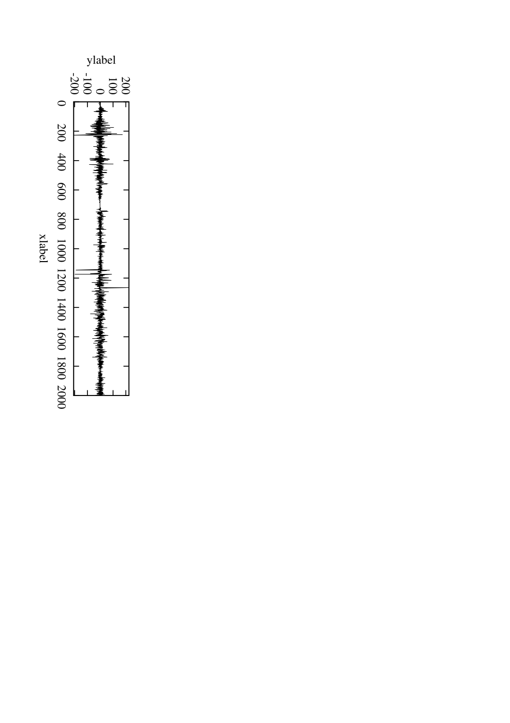
First we provide numerical justifications for the IID and Laplace assumptions introduced in previous subsections. We use the NREL dataset for the 50 highest power density offshore wind sites in California. We assume that the variations in demand are much smaller than in the wind power, which is justified by the high penetration scenario assumed this paper (also see Figure 2.3). Hence, we assume the net renewable generation error in our model is equal to the wind power prediction error. Since the dataset we use does not include forecast data, we use a simple linear predictor. Figure 3.4 plots the total power output of the 50 sites over a two-week period. Figures 3.4 and 3.4 plot the 10-minute-ahead prediction and the prediction error sequences for the same two-week period, respectively.

To test the IID assumption, we generated a sequence of IID random variables distributed according to the empirical marginal distribution of the prediction error sequence from the NREL dataset. Figure 3.4 compares the expected average fast-ramping generation costs for the NREL dataset and the IID sequence using policy $\pi^{(1)}$ . The maximum absolute difference between costs for the NREL dataset and for the IID sequence normalized by the NREL dataset cost is less than 3% and 6% for $\alpha=60\%$ and $\alpha=80\%$ , respectively.

To test the Laplace assumption, in Figure 3.4 we compare the empirical pdf of the prediction error dataset to the best fit Laplace distribution. The maximum absolute difference between the empirical cdf of the prediction error and the Laplace cdf is $0.018$ . Hence, the assumption of IID Laplace distributed net renewable generation prediction error appears to be reasonable. In the following, we will further corroborate this assumption with the NREL data using the average cost results.

Now we illustrate the results in Subsections 3.1 and 3.2. Figure 3.4 compares the minimum average costs in Proposition 3.2 and using the three-year simulated wind data for various values of power storage capacities and round-trip storage efficiencies $\alpha=60\%$ and $80\%$ . The maximum absolute difference between the theoretical and the simulated costs normalized by the theoretical cost is less than 6% and 8% for $\alpha=60\%$ and $\alpha=80\%$ , respectively. Thus, the Laplace distribution appears to be an acceptable approximation of the simulated wind generation data from NREL. Note that $80\%$ of the reduction for unlimited power storage capacity can be achieved with power storage capacity less than 4 standard deviations of the prediction error, which is equivalent to 13.9 MW-h.

Figure 3.4 compares the empirical pdf of the stored power of the simulated wind generation data to the stationary pdf under the Laplace distribution assumption in Proposition 3.3. The corresponding empirical pdf of the fast-ramping generation and its stationary pdf are shown in Figure 3.4. Note again the simulation results corroborate well with the theory.

The loss of load probability depends on the tail of the cdf $F_{\Delta}$ of the net generation prediction error. However, the number of samples of the wind data is small, and thus it is difficult to compare the loss of load probabilities of the wind dataset and the Laplace-distributed prediction error sequence. To illustrate the loss of load probabilities for the residual power system, we will assume that the net generation prediction error sequence is distributed according to the corresponding best fit Laplace distribution. Then the expected loss of load probability can be expressed as

\displaystyle{\cal J}^{(2)}(\pi,S_{1})=\limsup_{n\to\infty}\frac{1}{n}\sum_{i=1}^{n}F_{\Delta}(-G_{\mathrm{max}}-\alpha_{\mathrm{d}}S_{i}),

where $F_{\Delta}$ is the cdf of the best fit Laplace distribution. Figure 3.4 compares the expected loss of load probabilities and using the three-year simulated wind data for various values of power storage capacities and round-trip storage efficiencies $\alpha=60\%$ and $80\%$ . For large $S_{\mathrm{max}}$ , the average loss of load probability decreases exponentially in $S_{\mathrm{max}}$ as expected in Proposition 3.5.

4 Two-threshold policy

In Section 2, we showed that the policy $\pi^{(1)}$ minimizes the expected average conventional (or fast-ramping) generation—storage is discharged before conventional generation is used and conventional generation is never used to charge storage. We also showed that the policy $\pi^{(2)}$ minimizes the average loss of load probability—conventional generation is used before storage is discharged and conventional generation is used to keep storage as full as possible. In this section, we propose a general two-threshold policy, which includes $\pi^{(1)}$ and $\pi^{(2)}$ as extreme special cases. This policy tries to keep the stored power above a charging threshold and tries not to discharge storage below a discharging threshold.

Let $0\leq S_{\mathrm{c}}\leq S_{\mathrm{d}}\leq S_{\mathrm{max}}$ . The two-threshold policy is characterized by a charging threshold $S_{\mathrm{c}}$ and a discharging threshold $S_{\mathrm{d}}$ as given in Table 4 and illustrated in Figure 4 for $S_{\mathrm{c}}<\alpha_{\mathrm{c}}G_{\mathrm{max}}$ . When the prediction error $\Delta\geq 0$ , the storage is charged as much as possible using excess net renewable generation. If the stored power after this charging is above $S_{\mathrm{c}}$ , then conventional generation is not used. However, if it is below $S_{\mathrm{c}}$ , then the storage is charged as close to $S_{\mathrm{c}}$ as possible using conventional generation. When the prediction error $\Delta<-G_{\mathrm{max}}$ , the storage must be discharged to balance the prediction error. If there is still unbalanced prediction error after the storage is discharged to $S_{\mathrm{d}}$ , then fast-ramping generation is used such that the stored power is as close to $S_{\mathrm{d}}$ as possible. When the prediction error $-G_{\mathrm{max}}\leq\Delta<0$ , the case where the stored power is either lower than $S_{\mathrm{c}}$ or higher than $S_{\mathrm{d}}$ is similar to the above cases. When the stored power is between $S_{\mathrm{c}}$ and $S_{\mathrm{d}}$ , only the fast-ramping generation is used to balance the prediction error, and the stored power is unchanged.

Note that the optimal policies $\pi^{(1)}$ and $\pi^{(2)}$ for the two extreme cases in Theorem 2.1 and 2.4 are special cases of this policy with thresholds $(0,0)$ and $(S_{\mathrm{max}},S_{\mathrm{max}})$ , respectively.

\TABLE

Two-threshold policy parameterized by $(S_{\mathrm{c}},S_{\mathrm{d}})$ . $\pi_{i}$ $G_{i}$ $C_{i}$ $D_{i}$ $S_{i+1}$ $\displaystyle\frac{S_{\mathrm{max}}-S_{i}}{\alpha_{\mathrm{c}}}\leq\Delta_{i}$ $0$ $\displaystyle\frac{S_{\mathrm{max}}-S_{i}}{\alpha_{\mathrm{c}}}$ $0$ $S_{\mathrm{max}}$ $\displaystyle\frac{S_{\mathrm{c}}-S_{i}}{\alpha_{\mathrm{c}}}\leq\Delta_{i}<\frac{S_{\mathrm{max}}-S_{i}}{\alpha_{\mathrm{c}}}$ $0$ $\Delta_{i}$ $0$ $S_{i}+\alpha_{\mathrm{c}}\Delta_{i}$ $\displaystyle\frac{S_{\mathrm{c}}-S_{i}}{\alpha_{\mathrm{c}}}-G_{\mathrm{max}}\leq\Delta_{i}<\frac{S_{\mathrm{c}}-S_{i}}{\alpha_{\mathrm{c}}}$ $\displaystyle\frac{S_{\mathrm{c}}-S_{i}}{\alpha_{\mathrm{c}}}-\Delta_{i}$ $\displaystyle\frac{S_{\mathrm{c}}-S_{i}}{\alpha_{\mathrm{c}}}$ $0$ $S_{\mathrm{c}}$ $\displaystyle-G_{\mathrm{max}}\leq\Delta_{i}<\frac{S_{\mathrm{c}}-S_{i}}{\alpha_{\mathrm{c}}}-G_{\mathrm{max}}$ $G_{\mathrm{max}}$ $G_{\mathrm{max}}+\Delta_{i}$ $0$ $S_{i}+\alpha_{\mathrm{c}}(G_{\mathrm{max}}+\Delta_{i})$ $-G_{\mathrm{max}}-\alpha_{\mathrm{d}}S_{i}\leq\Delta_{i}<-G_{\mathrm{max}}$ $G_{\mathrm{max}}$ $0$ $-G_{\mathrm{max}}-\Delta_{i}$ $\displaystyle S_{i}+\frac{G_{\mathrm{max}}+\Delta_{i}}{\alpha_{\mathrm{d}}}$ $\Delta_{i}<-G_{\mathrm{max}}-\alpha_{\mathrm{d}}S_{i}$ $G_{\mathrm{max}}$ $0$ $\alpha_{\mathrm{d}}S_{i}$ $0$ (a) $0\leq S_{i}<S_{\mathrm{c}}$ $\pi_{i}$ $G_{i}$ $C_{i}$ $D_{i}$ $S_{i+1}$ $\displaystyle\frac{S_{\mathrm{max}}-S_{i}}{\alpha_{\mathrm{c}}}\leq\Delta_{i}$ $0$ $\displaystyle\frac{S_{\mathrm{max}}-S_{i}}{\alpha_{\mathrm{c}}}$ $0$ $S_{\mathrm{max}}$ $\displaystyle 0\leq\Delta_{i}<\frac{S_{\mathrm{max}}-S_{i}}{\alpha_{\mathrm{c}}}$ $0$ $\Delta_{i}$ $0$ $S_{i}+\alpha_{\mathrm{c}}\Delta_{i}$ $-G_{\mathrm{max}}\leq\Delta_{i}<0$ $-\Delta_{i}$ $0$ $0$ $S_{i}$ $-G_{\mathrm{max}}-\alpha_{\mathrm{d}}S_{i}\leq\Delta_{i}<-G_{\mathrm{max}}$ $G_{\mathrm{max}}$ $0$ $-G_{\mathrm{max}}-\Delta_{i}$ $\displaystyle S_{i}+\frac{G_{\mathrm{max}}+\Delta_{i}}{\alpha_{\mathrm{d}}}$ $\delta<-G_{\mathrm{max}}-\alpha_{\mathrm{d}}S_{i}$ $G_{\mathrm{max}}$ $0$ $\alpha_{\mathrm{d}}S_{i}$ $0$ (b) $S_{\mathrm{c}}\leq S_{i}\leq S_{\mathrm{d}}$ $\pi_{i}$ $G_{i}$ $C_{i}$ $D_{i}$ $S_{i+1}$ $\displaystyle\frac{S_{\mathrm{max}}-S_{i}}{\alpha_{\mathrm{c}}}\leq\Delta_{i}$ $0$ $\displaystyle\frac{S_{\mathrm{max}}-S_{i}}{\alpha_{\mathrm{c}}}$ $0$ $S_{\mathrm{max}}$ $\displaystyle 0\leq\Delta_{i}<\frac{S_{\mathrm{max}}-S_{i}}{\alpha_{\mathrm{c}}}$ $0$ $\Delta_{i}$ $0$ $S_{i}+\alpha_{\mathrm{c}}\Delta_{i}$ $-\alpha_{\mathrm{d}}(S_{i}-S_{\mathrm{d}})\leq\Delta_{i}<0$ $0$ $0$ $-\Delta_{i}$ $S_{i}+\Delta_{i}/\alpha_{\mathrm{d}}$ $-\alpha_{\mathrm{d}}(S_{i}-S_{\mathrm{d}})-G_{\mathrm{max}}\leq\Delta_{i}<-\alpha_{\mathrm{d}}(S_{i}-S_{\mathrm{d}})$ $-\Delta_{i}-\alpha_{\mathrm{d}}(S_{i}-S_{\mathrm{d}})$ $0$ $\alpha_{\mathrm{d}}(S_{i}-S_{\mathrm{d}})$ $S_{\mathrm{d}}$ $-G_{\mathrm{max}}-\alpha_{\mathrm{d}}S_{i}\leq\Delta_{i}<-\alpha_{\mathrm{d}}(S_{i}-S_{\mathrm{d}})-G_{\mathrm{max}}$ $G_{\mathrm{max}}$ $0$ $-G_{\mathrm{max}}-\Delta_{i}$ $\displaystyle S_{i}+\frac{G_{\mathrm{max}}+\Delta_{i}}{\alpha_{\mathrm{d}}}$ $\Delta_{i}<-G_{\mathrm{max}}-\alpha_{\mathrm{d}}S_{i}$ $G_{\mathrm{max}}$ $0$ $\alpha_{\mathrm{d}}S_{i}$ $0$ (c) $S_{\mathrm{d}}<S_{i}\leq S_{\mathrm{max}}$

\FIGURE

Illustration of the two-threshold policy.

Next we consider the general weighted-sum average cost:

\displaystyle{\cal J}(\pi,S_{1})=\rho_{1}{\cal J}^{(1)}(\pi,S_{1})+\rho_{2}{\cal J}^{(2)}(\pi,S_{1}),

where $\rho_{1}\geq 0$ and $\rho_{2}\geq 0$ . In the following proposition, we show that the two-threshold policy is optimal for the residual power system dynamic program with the above general weighted-sum cost and two slots.

Proposition 4.1

If the pdf of the prediction error $f_{\Delta}$ increases on $(-\infty,0]$ , then there exist ${S_{\mathrm{c}}}_{i}$ and ${S_{\mathrm{d}}}_{i}$ such that $0\leq{S_{\mathrm{c}}}_{i}\leq{S_{\mathrm{d}}}_{i}\leq S_{\mathrm{max}}$ , and the optimal policy for the general residual power system dynamic program with two slots is the two-threshold policy with parameters $({S_{\mathrm{c}}}_{i},{S_{\mathrm{d}}}_{i})$ for time $i=1,2$ .

The proof of this proposition is given in Appendix 9.

To demonstrate the two-threshold policy, we implemented a dynamic programming method by discretizing the state space and then running the value iteration (Bertsekas 2007). For the values of $G_{\mathrm{max}}$ , $S_{\mathrm{max}}$ , $\rho_{0}$ , and $\rho_{1}$ used in the following numerical examples, we find that the policy obtained from the value iteration is a discretized two-threshold policy.

Tradeoff between ${\cal J}^{(1)}$ and ${\cal J}^{(2)}$ : Figure 4 shows the tradeoff between the fast-ramping generation and the loss of load probability for no storage and for storage capacities $S_{\mathrm{max}}=50$ MW and $S_{\mathrm{max}}=100$ MW with fast-ramping generation capacity $G_{\mathrm{max}}=160$ MW. Note that the results for the Laplace pdf corroborate very well with the simulated wind generation data. As shown in the figure the loss of load probability is improved by more than two orders of magnitude by using power storage capacity less than 5 standard deviations of the prediction error.

Tradeoff between $S_{\mathrm{max}}$ and $G_{\mathrm{max}}$ : In Figure 4, we compare the two ways of mitigating renewable energy variability; using fast-ramping generation and using fast-response storage. We fix the expected average fast-ramping generation at $3.6$ MW (corresponding to 80% maximum reduction in the fast-ramping generation) and the loss of load probability at $2\cdot 10^{-6}$ (corresponds to one loss of load event every 10 years). To achieve these goals with minimum power storage capacity, we need $G_{\mathrm{max}}=170$ MW and $S_{\mathrm{max}}=60$ MW. To reduce the fossil fuel generation and to achieve the same goals, we can replace 1 MW of $G_{\mathrm{max}}$ with 1.3 MW of $S_{\mathrm{max}}$ .

5 Constrained $C_{\mathrm{max}}$ and $D_{\mathrm{max}}$

In previous sections, we assumed the rated storage power conversion $C_{\mathrm{max}}$ and the rated storage output power $D_{\mathrm{max}}$ to be unconstrained. In this section, we relax this condition and show that Theorems 2.1 and 2.4 can be extended to find the optimal policies with constraints on $C_{\mathrm{max}}$ and $D_{\mathrm{max}}$ .

Consider stochastic program I with the additional constraints

\displaystyle C_{\mathrm{max}}

\displaystyle\leq\frac{1}{\alpha_{\mathrm{c}}}S_{\mathrm{max}},\qquad D_{\mathrm{max}}\leq\alpha_{\mathrm{d}}S_{\mathrm{max}}.

(8)

In this following, we show that the optimal policy is a slight generalization of the policy for the unconstrained case in Theorem 2.1.

Theorem 5.1

The optimal policy $\pi^{(3)}$ for stochastic program I with constrained $C_{\mathrm{max}}$ and $D_{\mathrm{max}}$ is equal to

\displaystyle C_{i}^{(3)}

\displaystyle=\min\{C^{(1)}_{i},C_{\mathrm{max}}\},\qquad D_{i}^{(3)}=\min\{D^{(1)}_{i},D_{\mathrm{max}}\},\qquad G_{i}^{(3)}=\min\{[C_{i}^{(3)}-D_{i}^{(3)}-\Delta_{i}]^{+},G_{\mathrm{max}}\}.

The proof of this theorem is given in Appendix 7. Note that the above optimal policy reduces to the policy in Theorem 2.1 when $\alpha_{\mathrm{c}}C_{\mathrm{max}}=D_{\mathrm{max}}/\alpha_{\mathrm{d}}=S_{\mathrm{max}}$ .

Similarly, we can consider stochastic program II with constraints in (8) and obtain a generalization of the policy for the unconstrained case in Theorem 2.4.

Theorem 5.2

The optimal policy $\pi^{(4)}$ for stochastic program II with constrained $C_{\mathrm{max}}$ and $D_{\mathrm{max}}$ is equal to

\displaystyle C_{i}^{(4)}

\displaystyle=\min\{C^{(2)}_{i},C_{\mathrm{max}}\},\qquad D_{i}^{(4)}=\min\{D^{(2)}_{i},D_{\mathrm{max}}\},\qquad G_{i}^{(4)}=\min\{[C_{i}^{(4)}-D_{i}^{(4)}-\Delta_{i}]^{+},G_{\mathrm{max}}\}.

The proof of this theorem is given in Appendix 7.

Figure 5 plots the minimum average conventional generation versus $\alpha_{\mathrm{c}}C_{\mathrm{max}}/S_{\mathrm{max}}=D_{\mathrm{max}}/\alpha_{\mathrm{d}}S_{\mathrm{max}}$ for the NREL wind dataset and the CAISO load dataset. Note that most of the reduction in conventional generation in the unconstrained case can be achieved by $C_{\mathrm{max}}$ and $D_{\mathrm{max}}$ less than $5\%$ of $S_{\mathrm{max}}$ .

Figure 5 plots the minimum expected average loss of load probability versus $\alpha_{\mathrm{c}}C_{\mathrm{max}}/S_{\mathrm{max}}=D_{\mathrm{max}}/\alpha_{\mathrm{d}}S_{\mathrm{max}}$ . Note that loss of load may occur even when the stored power is high due to constrained $D_{\mathrm{max}}$ . Thus, the loss of load probability can be much higher for small $C_{\mathrm{max}}$ and $D_{\mathrm{max}}$ than for the unconstrained case.

6 Conclusion

This paper aimed to answer questions concerning the limits on the benefit of energy storage to renewable energy: How much can storage help? how much storage is needed? and what are the optimal control strategies for storage? To answer these questions, we formulated a single-bus power system with storage as stochastic program and established the optimal policies when the cost function is the expected average conventional generation and when it is the expected average loss of load probability. We proposed a general two-threshold policy for which these optimal policies are extreme special cases. We obtained refined analytical results by considering the multi-timescale operation of the grid. The results lead to the following potentially useful conclusions:

•

Using energy storage reduces fast-ramping generation by a factor up to the reciprocal of the round-trip inefficiency.
•

80% of the reduction in fast-ramping generation can be achieved using storage capacity equal to only four standard deviations of the net renewable generation prediction error.
•

The loss of load probability can be reduced by an unbounded factor as the energy storage capacity increases.
•

The loss of load probability can be reduced by an order of magnitude using storage capacity equal to only two standard deviations of the prediction error.
•

The Laplace distribution, which makes the analysis far more tractable, appears to be a reasonable approximation of the short time-scale prediction error of wind energy generation.
•

Most reduction in conventional generation for unconstrained charging and discharging rates can be achieved by relatively small such rates.

We corroborated our assumptions and analytical results with simulated wind data.

There are many open questions suggested by this work: What is the minimum expected average fast-ramping generation for constrained $C_{\mathrm{max}}$ and $D_{\mathrm{max}}$ under the Laplace assumption? What is the minimum expected average loss of load probability for limited $G_{\mathrm{max}}$ and $S_{\mathrm{max}}$ ? What is the natural cost function for which the two-threshold policy is optimal? What is the optimal policy when the ramping constraints of the fast-ramping generation are considered?

{APPENDICES}

7 Proofs for the single-bus power system results

Proof 7.1

Proof of Theorems 2.1 and 5.1. Since Theorem 2.1 is a special case of Theorem 5.1, we only need to prove the general case. Note that the proof of Lemma 2.2 holds for constrained $C_{\mathrm{max}}$ and $D_{\mathrm{max}}$ since the policies in (2) and (3) have smaller charging and discharging power than the optimal policies. Thus, we only need to show that for any policy $\pi_{k-1}$ ,

	$\displaystyle J_{k-1}$	$\displaystyle=G_{k-1}+J^{(1)}_{k}\left(\pi^{*},S_{k-1}+\alpha_{\mathrm{c}}C_{k-1}-\frac{1}{\alpha_{\mathrm{d}}}D_{k-1}\right)$
		$\displaystyle\geq G^{(1)}_{k-1}+J^{(1)}_{k}\left(\pi^{*},S_{k-1}+\alpha_{\mathrm{c}}C^{(1)}_{k-1}-\frac{1}{\alpha_{\mathrm{d}}}D^{(1)}_{k-1}\right)=J^{(1)}_{k-1}.$

Now we consider the following seven cases.

1.

$(S_{\mathrm{max}}-S_{k-1})/\alpha_{\mathrm{c}}\leq\Delta_{k-1}$ and $S_{\mathrm{max}}-\alpha_{\mathrm{c}}C_{\mathrm{max}}\leq S_{k-1}$ . By Lemma 2.2,

$\displaystyle J_{k-1}\geq J^{(1)}_{k}(\pi^{*},S_{\mathrm{max}})=J^{(1)}_{k-1}.$
2.

$C_{\mathrm{max}}\leq\Delta_{k-1}$ and $S_{k-1}<S_{\mathrm{max}}-\alpha_{\mathrm{c}}C_{\mathrm{max}}$ . By Lemma 2.2,

$\displaystyle J_{k-1}\geq J^{(1)}_{k}(\pi^{*},S_{k-1}+\alpha_{\mathrm{c}}C_{\mathrm{max}})=J^{(1)}_{k-1}.$

$0\leq\Delta_{k-1}\leq\min\{(S_{\mathrm{max}}-S_{k-1})/\alpha_{\mathrm{c}},C_{\mathrm{max}}\}$ .

•

If $\alpha C_{k-1}-D_{k-1}\leq\alpha C^{(1)}_{k-1}-D^{(1)}_{k-1}$ , then by Lemma 2.2,

\displaystyle J_{k-1}\geq J^{(1)}_{k}\left(\pi^{*},S_{k-1}+\alpha_{\mathrm{c}}C^{(1)}_{k-1}-\frac{1}{\alpha_{\mathrm{d}}}D^{(1)}_{k-1}\right)=J^{(1)}_{k-1}.

•

If $\alpha C_{k-1}-D_{k-1}>\alpha C^{(1)}_{k-1}-D^{(1)}_{k-1}$ , then by Lemma 2.2,

	$\displaystyle J_{k-1}-J^{(1)}_{k-1}$	$\displaystyle\geq C_{k-1}-\Delta_{k-1}-D_{k-1}$
		$\displaystyle\qquad-\alpha_{\mathrm{d}}\left(\alpha_{\mathrm{c}}(C_{k-1}-\Delta_{k-1})-\frac{1}{\alpha_{\mathrm{d}}}D_{k-1}\right)\geq 0.$

4.

$-\min\{\alpha_{\mathrm{d}}S_{k-1},D_{\mathrm{max}}\}\leq\Delta_{k-1}<0$ . The proof is the same as the previous case.

$-G_{\mathrm{max}}-\alpha_{\mathrm{d}}S_{k-1}\leq\Delta_{k-1}<-\alpha_{\mathrm{d}}S_{k-1}$ and $S_{k-1}\leq D_{\mathrm{max}}/\alpha_{\mathrm{d}}$ . By Lemma 2.2,

	$\displaystyle J_{k-1}-J^{(1)}_{k-1}$	$\displaystyle\geq C_{k-1}-D_{k-1}+\alpha_{\mathrm{d}}S_{k-1}$
		$\displaystyle\qquad-\alpha_{\mathrm{d}}\left(S_{k-1}+\alpha_{\mathrm{c}}C_{k-1}-\frac{1}{\alpha_{\mathrm{d}}}D_{k-1}\right)\geq 0.$

$-G_{\mathrm{max}}-D_{\mathrm{max}}\leq\Delta_{k-1}<-D_{\mathrm{max}}$ and $D_{\mathrm{max}}/\alpha_{\mathrm{d}}<S_{k-1}$ .

	$\displaystyle J_{k-1}-J^{(1)}_{k-1}$	$\displaystyle\geq C_{k-1}-D_{k-1}+D_{\mathrm{max}}$
		$\displaystyle\qquad-\alpha_{\mathrm{d}}\left(\alpha_{\mathrm{c}}C_{k-1}-\frac{1}{\alpha_{\mathrm{d}}}(D_{k-1}-D_{\mathrm{max}})\right)\geq 0.$

7.

$\Delta_{k-1}<-G_{\mathrm{max}}-\min\{\alpha_{\mathrm{d}}S_{k-1},D_{\mathrm{max}}\}$ . By the definition of loss of load, $J_{k-1}=J^{(1)}_{k-1}$ .

By induction we show that the stationary policy $\pi^{(1)}$ is optimal for the finite horizon stochastic program. Then for any $n\in\mathbb{N}$ and policy $\pi$ , we have

\displaystyle\frac{1}{n}J^{(1)}_{1}(\pi^{(1)},S_{1})\leq\frac{1}{n}J^{(1)}_{1}(\pi,S_{1}),

and thus

\displaystyle J^{(1)}(\pi^{(1)},S_{1})=\limsup_{n\to\infty}\frac{1}{n}J^{(1)}_{1}(\pi^{(1)},S_{1})\leq\limsup_{n\to\infty}\frac{1}{n}J^{(1)}_{1}(\pi,S_{1})=J^{(1)}(\pi,S_{1}).

Proof 7.2

Proof of Theorems 2.4 and 5.2. Since Theorem 2.4 is a special case of Theorem 5.2, we only need to prove the general case. Note that the property of the cost-to-go function in (5) holds for constrained $C_{\mathrm{max}}$ and $D_{\mathrm{max}}$ since the policy in (2) have smaller charging and discharging power than the optimal policy. Thus, we need to show that for any policy $\pi_{k-1}$ ,

	$\displaystyle J_{k-1}$	$\displaystyle=1_{\{\Delta_{k-1}<-G_{\mathrm{max}}-\alpha_{\mathrm{d}}S_{k-1}\}}+J^{(2)}_{k}\left(\pi^{*},S_{k-1}+\alpha_{\mathrm{c}}C_{k-1}-\frac{1}{\alpha_{\mathrm{d}}}D_{k-1}\right)$
		$\displaystyle\geq 1_{\{\Delta_{k-1}<-G_{\mathrm{max}}-\alpha_{\mathrm{d}}S_{k-1}\}}+J^{(2)}_{k}\left(\pi^{*},S_{k-1}+\alpha_{\mathrm{c}}C^{(2)}_{k-1}-\frac{1}{\alpha_{\mathrm{d}}}D^{(2)}_{k-1}\right)=J^{(2)}_{k-1}.$

Since the first terms in $J_{k-1}$ and $J^{(2)}_{k-1}$ are equal, by (5), we only need to show that

	$\displaystyle S_{k}$	$\displaystyle=S_{k-1}+\alpha_{\mathrm{c}}C_{k-1}-\frac{1}{\alpha_{\mathrm{d}}}D_{k-1}$
		$\displaystyle\geq S_{k-1}+\alpha_{\mathrm{c}}C^{(2)}_{k-1}-\frac{1}{\alpha_{\mathrm{d}}}D^{(2)}_{k-1}=S^{(2)}_{k}.$

Now we consider the following seven cases.

1.

If $(S_{\mathrm{max}}-S_{k-1})/\alpha_{\mathrm{c}}-G_{\mathrm{max}}\leq\Delta_{k-1}$ and $S_{\mathrm{max}}-\alpha_{\mathrm{c}}C_{\mathrm{max}}\leq S_{k-1}$ , then $S_{k}\leq S_{\mathrm{max}}=S^{(2)}_{k}$ .
2.

If $C_{\mathrm{max}}-G_{\mathrm{max}}\leq\Delta_{k-1}$ and $S_{k-1}<S_{\mathrm{max}}-\alpha_{\mathrm{c}}C_{\mathrm{max}}$ , then $S_{k}\leq S_{k-1}+\alpha_{\mathrm{c}}C_{\mathrm{max}}=S^{(2)}_{k}$ .

If $-G_{\mathrm{max}}\leq\Delta_{k-1}<\min\{(S_{\mathrm{max}}-S_{k-1})/\alpha_{\mathrm{c}},C_{\mathrm{max}}\}-G_{\mathrm{max}}$ , then

	$\displaystyle S_{k}$	$\displaystyle\leq S_{k-1}+\alpha_{\mathrm{c}}(G_{k-1}+D_{k-1}+\Delta_{k-1})-\frac{1}{\alpha_{\mathrm{d}}}D_{k-1}$
		$\displaystyle\leq S_{k-1}+\alpha_{\mathrm{c}}(G_{\mathrm{max}}+\Delta_{k-1})=S^{(2)}_{k}.$

If $-\min\{\alpha_{\mathrm{d}}S_{k-1},D_{\mathrm{max}}\}-G_{\mathrm{max}}\leq\Delta_{k-1}<-G_{\mathrm{max}}$ , then

	$\displaystyle S_{k}$	$\displaystyle\leq S_{k-1}+\alpha_{\mathrm{c}}C_{k-1}-\frac{1}{\alpha_{\mathrm{d}}}(-G_{k-1}+C_{k-1}-\Delta_{k-1})$
		$\displaystyle\leq S_{k-1}-\frac{1}{\alpha_{\mathrm{d}}}(-G_{\mathrm{max}}-\Delta_{k-1})=S^{(2)}_{k}.$

5.

If $\Delta_{k-1}<-G_{\mathrm{max}}-\min\{\alpha_{\mathrm{d}}S_{k-1},D_{\mathrm{max}}\}$ , then $S_{k}=S^{(2)}_{k}=S_{k-1}-\min\{S_{k-1},D_{\mathrm{max}}/\alpha_{\mathrm{d}}\}$ .

By induction we show that the stationary policy $\pi^{(2)}$ is optimal for the finite horizon stochastic program. Then for any $n\in\mathbb{N}$ and policy $\pi$ , we have

\displaystyle\frac{1}{n}J^{(2)}_{1}(\pi^{(2)},S_{1})\leq\frac{1}{n}J^{(2)}_{1}(\pi,S_{1}),

and thus

\displaystyle J^{(2)}(\pi^{(2)},S_{1})=\limsup_{n\to\infty}\frac{1}{n}J^{(2)}_{1}(\pi^{(2)},S_{1})\leq\limsup_{n\to\infty}\frac{1}{n}J^{(2)}_{1}(\pi,S_{1})=J^{(2)}(\pi,S_{1}).

8 Proofs for the residual power system results

We first establish bounds on the expected stored power.

Lemma 8.1

Suppose that $S_{i+1}=\max\{S_{i}+\Theta_{i},0\}$ for $i=1,2,\ldots,n$ , where $S_{1}\geq 0$ is given and $\Theta_{i}$ , $i=1,2,\ldots,n$ , is a sequence of IID random variables with mean $\mu_{\Theta}$ and variance $\sigma_{\Theta}^{2}$ .

1.

If $\mu_{\Theta}\leq 0$ , then $\E[S_{k+1}]\leq\sqrt{k(\mu_{\Theta}^{2}+\sigma_{\Theta}^{2})+S_{1}^{2}}$ .
2.

If $\mu_{\Theta}>0$ , then $S_{1}+k\mu_{\Theta}\leq\E[S_{k+1}]\leq k\mu_{\Theta}+\sqrt{k}\log_{2}(4k)\sqrt{\sigma_{\Theta}^{2}+S_{1}^{2}/k}$ .

Proof 8.2

For $\mu_{\Theta}\leq 0$ , consider

	$\displaystyle\E[S_{k+1}^{2}]$	$\displaystyle\leq\E[(S_{k}+\Theta_{k})^{2}]$
		$\displaystyle=\E[S_{k}^{2}]+2\E[S_{k}]\E[\Theta_{k}]+\E[\Theta_{k}^{2}]$
		$\displaystyle\leq\E[S_{k}^{2}]+(\mu_{\Theta}^{2}+\sigma_{\Theta}^{2})$
		$\displaystyle\leq S_{1}^{2}+k(\mu_{\Theta}^{2}+\sigma_{\Theta}^{2}),$

where the equality follows by the independence between $\Theta_{k}$ and $(\Theta_{1},\Theta_{2},\ldots,\Theta_{k-1})$ and the last inequality follows by induction. Thus, by Jensen’s inequality,

\displaystyle\E[S_{k+1}]\leq\sqrt{\E[S_{k+1}^{2}]}\leq\sqrt{k(\mu_{\Theta}^{2}+\sigma_{\Theta}^{2})+S_{1}^{2}}.

For $\mu_{T}>0$ , the expected stored power can be lower bounded as

\displaystyle\E[S_{k+1}]\geq\E[S_{k}+\Theta_{k}]\geq S_{1}+k\mu_{\Theta},

where the last inequality follows by induction. Next, we consider

	$\displaystyle\E[S_{k+1}-k\mu_{\Theta}]$	$\displaystyle=\E[\max\{S_{k}+\Theta_{k},0\}-k\mu_{\Theta}]$
		$\displaystyle=\E\left[\max\left\{0,\ S_{1}+\sum_{i=1}^{k}\Theta_{i},\ \max_{2\leq j\leq k}\sum_{i=j}^{k}\Theta_{i}\right\}-k\mu_{\Theta}\right]$
		$\displaystyle\leq\E\left[\max_{1\leq j\leq k}\left\|\sum_{i=j}^{k}\tilde{\Theta}_{i}\right\|\right],$

where $\tilde{\Theta}_{i}=\Theta_{i}-\mu_{\Theta}$ for $i=2,3,\ldots,k$ and $\tilde{\Theta}_{1}=S_{1}+\Theta_{1}-\mu_{\Theta}$ . Note that $\E[\Theta_{i}\Theta_{j}]=0$ for $i\neq j$ . By the inequality in Doob (1953, Lemma 4.1), we have

\displaystyle\E\left[\max_{1\leq j\leq k}\left|\sum_{i=j}^{k}\tilde{\Theta}_{i}\right|^{2}\right]\leq\log_{2}(4k)^{2}(k\sigma_{\Theta}^{2}+S_{1}^{2}).

Therefore,

	$\displaystyle\E[S_{k+1}]$	$\displaystyle\leq\E\left[\max_{1\leq j\leq k}\left\|\sum_{i=j}^{k}\tilde{\Theta}_{i}\right\|\right]+k\mu_{\Theta}\leq\sqrt{\E\left[\left(\max_{1\leq j\leq k}\left\|\sum_{i=j}^{k}\tilde{\Theta}_{i}\right\|\right)^{2}\right]}+k\mu_{\Theta}$
		$\displaystyle=\sqrt{\E\left[\max_{1\leq j\leq k}\left\|\sum_{i=j}^{k}\tilde{\Theta}_{i}\right\|^{2}\right]}+k\mu_{\Theta}\leq\sqrt{k}\log_{2}(4k)\sqrt{\mu_{\Theta}^{2}+S_{1}^{2}/k}+k\mu_{\Theta},$

where the second inequality follows by Jensen’s inequality.

Proof 8.3

Proof of Propositions 3.1 and 3.6. Since Proposition 3.1 is a special case of Proposition 3.6, we only need to prove the general case. For unlimited $G_{\mathrm{max}}$ and $S_{\mathrm{max}}$ , the optimal policy $\pi^{(1)}$ satisfies

	$\displaystyle 0$	$\displaystyle=G_{i}-C_{i}+D_{i}+\Delta_{i},$
	$\displaystyle S_{i+1}$	$\displaystyle=S_{i}+\alpha_{\mathrm{c}}C_{i}-\frac{1}{\alpha_{\mathrm{d}}}D_{i},$

for $i=1,2,\ldots$ . Note that $C_{i}=\Delta_{i}^{+}$ . Now we consider

	$\displaystyle\frac{1}{n}\sum_{i=1}^{n}G_{i}$	$\displaystyle=\frac{1}{n}\sum_{i=1}^{n}(C_{i}-D_{i}-\Delta_{i})$
		$\displaystyle=\frac{1}{n}\sum_{i=1}^{n}\left((1-\alpha)C_{i}-\Delta_{i}\right)+\frac{1}{n}\alpha_{\mathrm{d}}(S_{n+1}-S_{1})$
		$\displaystyle=\frac{1}{n}\sum_{i=1}^{n}\left((1-\alpha)\Delta_{i}^{+}-\Delta_{i}\right)+\frac{1}{n}\alpha_{\mathrm{d}}(S_{n+1}-S_{1})$
		$\displaystyle=\frac{1}{n}\sum_{i=1}^{n}\left(\Delta_{i}^{-}-\alpha\Delta_{i}^{+}\right)+\frac{1}{n}\alpha_{\mathrm{d}}(S_{n+1}-S_{1}).$

Next let $\Theta_{i}=\alpha_{\mathrm{c}}\Delta_{i}^{+}-\Delta_{i}^{-}/\alpha_{\mathrm{d}}$ for $i=1,2,\ldots$ , which is sequence of IID random variables with mean $\mu_{\Theta}=\E[\Theta_{i}]$ and variance $\sigma_{\Theta}^{2}=\Var[\Theta_{i}]$ . Suppose that $\mu_{\Theta}\geq 0$ . We only need to show that $\limsup_{n\to\infty}\E[S_{n+1}/n]=0$ since

\displaystyle\limsup_{n\to\infty}\E\left[\frac{1}{n}\sum_{i=1}^{n}\left(\Delta_{i}^{-}-\alpha\Delta_{i}^{+}\right)-\frac{1}{n}\alpha_{\mathrm{d}}S_{1}\right]=\E[\Delta^{-}-\alpha\Delta^{+}].

By Lemma 8.1, we have

\displaystyle 0

\displaystyle\leq\limsup_{n\to\infty}\E\left[\frac{1}{n}S_{n+1}\right]\leq\limsup_{n\to\infty}\frac{1}{n}\sqrt{n(\mu_{\Theta}^{2}+\sigma_{\Theta}^{2})+S_{1}^{2}}=0.

Suppose that $\mu_{\Theta}<0$ . By Lemma 8.1, we have

	$\displaystyle\limsup_{n\to\infty}\E\left[\frac{1}{n}\sum_{i=1}^{n}G_{i}\right]$	$\displaystyle\leq\E\left[\Delta^{-}-\alpha\Delta^{+}\right]+\limsup_{n\to\infty}\frac{1}{n}\alpha_{\mathrm{d}}\left(n\mu_{\Theta}+\sqrt{n}\log_{2}(4k)\sqrt{\sigma_{\Theta}^{2}+S_{1}^{2}/n}\right)$
		$\displaystyle=\E\left[\Delta^{-}-\alpha\Delta^{+}\right]+\alpha_{\mathrm{d}}\mu_{\Theta}=0.$

Proof 8.4

Proof of Proposition 3.2. To find the expected average fast-ramping generation ${\cal J}^{(1)}(\pi^{(1)},S_{1})$ under the Laplace assumption, we need to show that there exist a constant $\eta$ and a function $v(s)$ such that

\displaystyle\eta+v(s)

\displaystyle=\E\left[G^{(1)}+v\left(s+\alpha_{\mathrm{c}}C^{(1)}-\frac{1}{\alpha_{\mathrm{d}}}D^{(1)}\right)\right],

(9)

and $\lim_{n\to\infty}\E\left[v(S_{n})/n\right]=0$ Arapostathis et al. (1993). Then the average cost is equal to $\eta$ . Now we verify that for the policy $\pi^{(1)}$ in Theorem 2.1,

	$\displaystyle\eta$	$\displaystyle=\frac{1}{2\lambda}\left(\frac{(1-\alpha)(1-e^{-\lambda G_{\mathrm{max}}})}{1-\alpha e^{-(1/\alpha_{\mathrm{c}}-\alpha_{\mathrm{d}})\lambda S_{\mathrm{max}}/2}}\right),$
	$\displaystyle v(s)$	$\displaystyle=-\left(\frac{\alpha_{\mathrm{d}}(1-e^{-\lambda G_{\mathrm{max}}})}{1-\alpha e^{-(1/\alpha_{\mathrm{c}}-\alpha_{\mathrm{d}})\lambda S_{\mathrm{max}}/2}}\right)s+\frac{1}{\lambda}\left(\frac{1+\alpha}{1-\alpha}\right)\left(\frac{\alpha e^{-(1/\alpha_{\mathrm{c}}-\alpha_{\mathrm{d}})\lambda(S_{\mathrm{max}}-s)/2}}{1-\alpha e^{-(1/\alpha_{\mathrm{c}}-\alpha_{\mathrm{d}})\lambda S_{\mathrm{max}}/2}}\right)(1-e^{-\lambda G_{\mathrm{max}}})$

satisfy

	$\displaystyle\eta+v(s)$	$\displaystyle=\E\left[G^{(1)}+v\left(s+\alpha_{\mathrm{c}}C^{(1)}-\frac{1}{\alpha_{\mathrm{d}}}D^{(1)}\right)\right]$
		$\displaystyle=\E\left[v(S_{\mathrm{max}});\frac{1}{\alpha_{\mathrm{c}}}(S_{\mathrm{max}}-s)\leq\Delta\right]+\E\left[v(s+\alpha_{\mathrm{c}}\Delta);0\leq\Delta<\frac{1}{\alpha_{\mathrm{c}}}(S_{\mathrm{max}}-s)\right]$
		$\displaystyle\qquad+\E\left[v\left(s+\frac{1}{\alpha_{\mathrm{d}}}\Delta\right);-\alpha_{\mathrm{d}}s\leq\Delta<0\right]+\E\left[-\Delta-\alpha_{\mathrm{d}}s+v(0);-G_{\mathrm{max}}-\alpha_{\mathrm{d}}s\leq\Delta<-\alpha_{\mathrm{d}}s\right]$
		$\displaystyle\qquad+\E\left[G_{\mathrm{max}}+v(0);\Delta<-G_{\mathrm{max}}-\alpha_{\mathrm{d}}s\right],$

where for random variable $X$ and a set $A$ we define $\E[X;A]=\E[X|A]\P(A)$ . Furthermore, $v(s)$ is bounded for $s\in[0,S_{\mathrm{max}}]$ , and thus $\lim_{n\to\infty}\E\left[v(S_{n})/n\right]=0$ .

Proof 8.5

Proof of Proposition 3.3. Since the optimal policy $\pi^{(1)}$ in Theorem 2.1 is stationary, the corresponding stored power sequence is a Markov process

\displaystyle S_{i+1}

\displaystyle=\begin{cases}S_{\mathrm{max}}&\text{if}\ (S_{\mathrm{max}}-S_{i})/\alpha_{\mathrm{c}}\leq\Delta_{i}\\ S_{i}+\alpha_{\mathrm{c}}\Delta_{i}&\text{if}\ 0\leq\Delta_{i}<(S_{\mathrm{max}}-S_{i})/\alpha_{\mathrm{c}}\\ S_{i}+\Delta_{i}/\alpha_{\mathrm{d}}&\text{if}\ -\alpha_{\mathrm{d}}S_{i}\leq\Delta_{i}<0\\ 0&\text{if}\ \Delta_{i}<-\alpha_{\mathrm{d}}S_{i}.\end{cases}

Let $F_{i}$ be the cdf of $S_{i}$ . Then for $0\leq s<S_{\mathrm{max}}$ ,

	$\displaystyle F_{i+1}(s)$	$\displaystyle=\int_{-\infty}^{-\alpha_{\mathrm{d}}(S_{\mathrm{max}}-s)}\frac{\lambda}{2}e^{\lambda\delta}F_{i}(S_{\mathrm{max}})d\delta+\int_{-\alpha_{\mathrm{d}}(S_{\mathrm{max}}-s)}^{0}\frac{\lambda}{2}e^{\lambda\delta}F_{i}(s-\delta/\alpha_{\mathrm{d}})d\delta$
		$\displaystyle\qquad+\int_{0}^{(1/\alpha_{\mathrm{c}})s}\frac{\lambda}{2}e^{-\lambda\delta}F_{i}(s-\alpha_{\mathrm{c}}\delta)d\delta.$		(10)

For $s<0$ , $F_{i+1}(s)=0$ , and for $s\geq S_{\mathrm{max}}$ , $F_{i+1}(s)=1$ . Let

\displaystyle F_{S}(s)

\displaystyle=\begin{cases}0&\text{if}\ s<0\\ \displaystyle\frac{1}{1-\alpha e^{-(1/\alpha_{\mathrm{c}}-\alpha_{\mathrm{d}})\lambda S_{\mathrm{max}}/2}}\left(1-\frac{1+\alpha}{2}e^{-(1/\alpha_{\mathrm{c}}-\alpha_{\mathrm{d}})\lambda s/2}\right)&\text{if}\ 0\leq s<S_{\mathrm{max}}\\ 1&\text{if}\ s\geq S_{\mathrm{max}}\end{cases}.

It can be verified that (10) is satisfied with $F_{i}(s)=F_{i+1}(s)=F_{S}(s)$ for all $s$ . Now we only need to show that the Markov chain is irreducible with respect to $F_{S}(s)$ , which implies that the stationary distribution is unique (Gilks et al. 1995, Theorem 4.1). Let $S_{i}=s$ , and let $\mathcal{B}=(b_{1},b_{2})\subset[s,S_{\mathrm{max}}]$ such that $\P\{S\in\mathcal{B}\}>0$ under the stationary distribution, that is, $b_{2}>b_{1}$ . Then

\displaystyle\P\{S_{i+1}\in\mathcal{B}\}

\displaystyle=\int_{(1/\alpha_{\mathrm{c}})(b_{1}-s)}^{(1/\alpha_{\mathrm{c}})(b_{2}-s)}\frac{\lambda}{2}e^{-\lambda\delta}d\delta=\frac{1}{2}\left(e^{-(1/\alpha_{\mathrm{c}})\lambda(b_{1}-s)}-e^{-(1/\alpha_{\mathrm{c}})\lambda(b_{2}-s)}\right)>0.

If $\mathcal{B}=\{0\}$ , then

\displaystyle P\{S_{i+1}\in\mathcal{B}\}=\int_{-\infty}^{-\alpha_{\mathrm{d}}s}\frac{\lambda}{2}e^{\lambda\delta}d\delta=\frac{1}{2}e^{-\alpha_{\mathrm{d}}\lambda s}>0.

Similarly, $\P\{S_{i+1}\in\mathcal{B}\}>0$ for $\mathcal{B}=(b_{1},b_{2})\subset[0,s]$ and $\{S_{\mathrm{max}}\}$ . Thus, we can generalize $\mathcal{B}$ to any set such that $\P\{S\in\mathcal{B}\}>0$ . Therefore, the Markov chain is irreducible.

Using stationary distribution $F_{S}(s)$ above, we can find the corresponding distribution of the fast-ramping generation

	$\displaystyle F_{G}(g)$	$\displaystyle=1-\int_{-\infty}^{-g-\alpha_{\mathrm{d}}S_{\mathrm{max}}}\frac{\lambda}{2}e^{\lambda\delta}d\delta-\int_{-g-\alpha_{\mathrm{d}}S_{\mathrm{max}}}^{-g}\frac{\lambda}{2}e^{\lambda\delta}F_{S}\left(-\frac{1}{\alpha_{\mathrm{d}}}(\delta+g)\right)d\delta$
		$\displaystyle=1-\frac{1}{2}e^{-\lambda g-\lambda\alpha_{\mathrm{d}}S_{\mathrm{max}}}$
		$\displaystyle\qquad-\frac{1}{1-\alpha e^{-(1/\alpha_{\mathrm{c}}-\alpha_{\mathrm{d}})\lambda S_{\mathrm{max}}/2}}\left(\frac{1-\alpha}{2}e^{-\lambda g}-\frac{1}{2}e^{-\lambda g-\lambda\alpha_{\mathrm{d}}S_{\mathrm{max}}}+\frac{\alpha}{2}e^{-\lambda g-(1/\alpha_{\mathrm{c}}+\alpha_{\mathrm{d}})\lambda S_{\mathrm{max}}/2}\right)$
		$\displaystyle=1-\frac{1-\alpha}{2(1-\alpha e^{-(1/\alpha_{\mathrm{c}}-\alpha_{\mathrm{d}})\lambda S_{\mathrm{max}}/2})}e^{-\lambda g}$

for $g\geq 0$ , $F_{G}(g)=0$ for $g<0$ , and $F_{G}(g)=1$ for $g\geq G_{\mathrm{max}}$ .

Proof 8.6

Proof of Proposition 3.4. For any $u_{k+1}>0$ , consider

	$\displaystyle\E\left[1_{\{\Delta_{k+1}<-G_{\mathrm{max}}-\alpha_{\mathrm{d}}S_{k+1}\}}\right]$	$\displaystyle=\E\left[1_{\{\Delta_{k+1}<-G_{\mathrm{max}}-\alpha_{\mathrm{d}}S_{k+1}\}};\ S_{k+1}\leq u_{k+1}\right]$
		$\displaystyle\qquad+\E\left[1_{\{\Delta_{k+1}<-G_{\mathrm{max}}-\alpha_{\mathrm{d}}S_{k+1}\}};S_{k+1}>u_{k+1}\right]$
		$\displaystyle\leq\P\{S_{k+1}\leq u_{k+1}\}+\E\left[1_{\{\Delta_{k+1}<-G_{\mathrm{max}}-\alpha_{\mathrm{d}}u_{k+1}\}}\right]$
		$\displaystyle=\P\{S_{k+1}\leq u_{k+1}\}+F_{\Delta}(-G_{\mathrm{max}}-\alpha_{\mathrm{d}}u_{k+1})$

and choose $u_{k+1}=\E[S_{k+1}]/2$ . Then we have

	$\displaystyle\E\left[1_{\{\Delta_{k+1}<-G_{\mathrm{max}}-\alpha_{\mathrm{d}}S_{k+1}\}}\right]$	$\displaystyle\leq\P\left\{S_{k+1}<\frac{1}{2}\E[S_{k+1}]\right\}+F_{\Delta}\left(-G_{\mathrm{max}}-\frac{\alpha_{\mathrm{d}}\E[S_{k+1}]}{2}\right)$
		$\displaystyle=\P\left\{\E[S_{k+1}]-S_{k+1}>\frac{1}{2}\E[S_{k+1}]\right\}+F_{\Delta}\left(-G_{\mathrm{max}}-\frac{\alpha_{\mathrm{d}}\E[S_{k+1}]}{2}\right).$

For unlimited $S_{\mathrm{max}}$ , under the optimal policy $\pi^{(2)}$ in Theorem 2.4, we have

\displaystyle S_{k+1}

\displaystyle=\max\left\{S_{k}+\Theta_{k},0\right\},

where $\Theta_{k}=\alpha_{\mathrm{c}}(G_{\mathrm{max}}+\Delta_{k})^{+}-(1/\alpha_{\mathrm{d}})(G_{\mathrm{max}}+\Delta_{k})^{-}$ with $\mu_{\Theta}=\E[\Theta_{k}]>0$ and $\sigma_{\Theta}^{2}=\Var[\Theta_{k}]$ . Then by Lemma 8.1,

\displaystyle S_{1}+k\mu_{\Theta}\leq\E[S_{k+1}]\leq k\mu_{\Theta}+\sqrt{k}\log_{2}(4k)\sqrt{\sigma_{\Theta}^{2}+S_{1}^{2}/k}.

Thus,

	$\displaystyle\E\left[1_{\{\Delta_{k+1}<-G_{\mathrm{max}}-\alpha_{\mathrm{d}}S_{k+1}\}}\right]$	$\displaystyle\leq\P\left\{\left(\E[S_{k+1}]-S_{k+1}\right)^{2}>\frac{1}{4}\E[S_{k+1}]^{2}\right\}+F_{\Delta}\left(-G_{\mathrm{max}}-\frac{\alpha_{\mathrm{d}}}{2}(k\mu_{\Theta}+S_{1})\right)$
		$\displaystyle\leq\frac{4\Var(S_{k+1})}{\E[S_{k+1}]^{2}}+F_{\Delta}\left(-G_{\mathrm{max}}-\frac{\alpha_{\mathrm{d}}}{2}(k\mu_{\Theta}+S_{1})\right)$
		$\displaystyle\leq\frac{4\Var(S_{k+1})}{(k\mu_{\Theta}+S_{1})^{2}}+F_{\Delta}\left(-G_{\mathrm{max}}-\frac{\alpha_{\mathrm{d}}}{2}(k\mu_{\Theta}+S_{1})\right),$

where the second inequality follows by the Chebyshev’s inequality. Next we consider

	$\displaystyle\Var[S_{k+1}]$	$\displaystyle=\E[S_{k+1}^{2}]-\left(\E[S_{k+1}]\right)^{2}$
		$\displaystyle\leq\E\left[(S_{k}+\Theta_{k})^{2}\right]-(k\mu_{\Theta}+S_{1})^{2}$
		$\displaystyle=\E\left[S_{k}^{2}\right]+2\mu_{\Theta}\E[S_{k}]+(\mu_{\Theta}^{2}+\sigma_{\Theta}^{2})-(k\mu_{\Theta}+S_{1})^{2}$
		$\displaystyle\leq\E\left[S_{k}^{2}\right]+2\mu_{\Theta}\left((k-1)\mu_{\Theta}+\sqrt{k-1}\log_{2}(4(k-1))\sqrt{\sigma_{\Theta}^{2}+\frac{S_{1}^{2}}{k-1}}\right)+(\mu_{\Theta}^{2}+\sigma_{\Theta}^{2})-(k\mu_{\Theta}+S_{1})^{2}$
		$\displaystyle\leq\sum_{j=2}^{k}2\mu_{\Theta}\left((j-1)\mu_{\Theta}+\sqrt{j-1}\log_{2}(4(j-1))\sqrt{\sigma_{\Theta}^{2}+S_{1}^{2}}\right)+k(\mu_{\Theta}^{2}+\sigma_{\Theta}^{2})+S_{1}^{2}-(k\mu_{\Theta}+S_{1})^{2}$
		$\displaystyle=\sum_{j=2}^{k}2\mu_{\Theta}\sqrt{j-1}\log_{2}(4(j-1))\sqrt{\sigma_{\Theta}^{2}+S_{1}^{2}}+k(k-1)\mu_{\Theta}^{2}+k(\mu_{\Theta}^{2}+\sigma_{\Theta}^{2})+S_{1}^{2}-(k\mu_{\Theta}+S_{1})^{2}$
		$\displaystyle=\sum_{j=2}^{k}2\mu_{\Theta}\sqrt{j-1}\log_{2}(4(j-1))\sqrt{\sigma_{\Theta}^{2}+S_{1}^{2}}+k(\sigma_{\Theta}^{2}-2\mu_{\Theta}S_{1}),$

where the third inequality follows by induction. Since

	$\displaystyle\sum_{j=2}^{k}2\mu_{\Theta}\sqrt{\sigma_{\Theta}^{2}+S_{1}^{2}}\left(\sqrt{j-1}\frac{\ln 4(j-1)}{\ln 2}\right)$	$\displaystyle\leq 2\mu_{\Theta}\sqrt{\sigma_{\Theta}^{2}+S_{1}^{2}}\int_{1}^{k}\sqrt{x}\frac{\ln 4x}{\ln 2}dx$
		$\displaystyle=2\mu_{\Theta}\sqrt{\sigma_{\Theta}^{2}+S_{1}^{2}}\left(\left.\frac{2}{3\ln 2}x^{3/2}\ln 4x\right\|_{1}^{k}-\int_{1}^{k}\frac{2}{3\ln 2}x^{1/2}dx\right)$
		$\displaystyle\leq c_{1}k^{5/3},$

for some constant $c_{1}>0$ and for sufficiently large $k$ , we have

	$\displaystyle\limsup_{n\to\infty}\frac{1}{n}\sum_{k=1}^{n}\E\left[1_{\{\Delta_{k+1}<-G_{\mathrm{max}}-\alpha_{\mathrm{d}}S_{k+1}\}}\right]$	$\displaystyle\leq\limsup_{n\to\infty}\frac{1}{n}\sum_{k=1}^{n}\left(\frac{4\Var(S_{+1})}{(k\mu_{\Theta}+S_{1})^{2}}+F_{\Delta}\left(-G_{\mathrm{max}}-\frac{\alpha_{\mathrm{d}}}{2}(k\mu_{\Theta}+S_{1})\right)\right)$
		$\displaystyle\leq\limsup_{n\to\infty}\frac{1}{n}\left(c_{2}+c_{3}\sum_{k=k^{\prime}}^{n}\left(\frac{1}{k^{1/3}}+\frac{1}{k}\right)\right)=0,$

where $k^{\prime}$ , $c_{2}$ , and $c_{3}$ are constants.

Proof 8.7

Proof of Proposition 3.5. We first establish a lower bound on the expected loss of load probability. For power storage capacity $S_{\mathrm{max}}$ , ${\cal J}^{(2)}(\pi^{(2)},S_{1})$ is lower bounded by the expected loss of load probability associated with the stored power sequence $S_{i}=S_{\mathrm{max}}$ for $i=1,2,\ldots$ , that is,

\displaystyle{\cal J}^{(2)}(\pi^{(2)},S_{1})

\displaystyle\geq\limsup_{n\to\infty}\E\left[\frac{1}{n}\sum_{i=1}^{n}1_{\{\Delta_{i}<-G_{\mathrm{max}}-\alpha_{\mathrm{d}}S_{\mathrm{max}}\}}\right]=\frac{1}{2}e^{-\lambda G_{\mathrm{max}}-\alpha_{\mathrm{d}}\lambda S_{\mathrm{max}}}.

Thus,

\displaystyle\lim_{S_{\mathrm{max}}\to\infty}\frac{\ln{\cal J}^{(2)}(\pi^{(2)},S_{1})}{S_{\mathrm{max}}}\geq-\alpha_{\mathrm{d}}\lambda=\gamma_{\mathrm{min}}.

Next, we establish an upper bound on ${\cal J}^{(2)}(\pi,S_{1})$ by considering a suboptimal policy $\pi$ in Table 8.7. Let $F_{i}$ be the cdf of $S_{i}$ . Then for $0\leq s<S_{\mathrm{max}}$ ,

	$\displaystyle F_{i+1}(s)$	$\displaystyle=\int_{-\infty}^{-G_{\mathrm{max}}-\alpha_{\mathrm{d}}(S_{\mathrm{max}}-s)}\frac{\lambda}{2}e^{\lambda\delta}d\delta+\int_{-G_{\mathrm{max}}-\alpha_{\mathrm{d}}(S_{\mathrm{max}}-s)}^{-G_{\mathrm{max}}}\frac{\lambda}{2}e^{\lambda\delta}F_{i}\left(s-\frac{\delta+G_{\mathrm{max}}}{\alpha_{\mathrm{d}}}\right)d\delta$
		$\displaystyle\qquad+\int_{-G_{\mathrm{max}}}^{0}\frac{\lambda}{2}e^{\lambda\delta}F_{i}(s)d\delta+\int_{0}^{(1/\alpha_{\mathrm{c}})s}\frac{\lambda}{2}e^{-\lambda\delta}F_{i}(s-\alpha_{\mathrm{c}}\delta)d\delta$
		$\displaystyle=\frac{1}{2}e^{-\lambda G_{\mathrm{max}}-\alpha_{\mathrm{d}}\lambda(S_{\mathrm{max}}-s)}+\frac{1}{2}(1-e^{-\lambda G_{\mathrm{max}}})F_{i}(s)$
		$\displaystyle\qquad+\int_{-G_{\mathrm{max}}-\alpha_{\mathrm{d}}(S_{\mathrm{max}}-s)}^{-G_{\mathrm{max}}}\frac{\lambda}{2}e^{\lambda\delta}F_{i}\left(s-\frac{\delta+G_{\mathrm{max}}}{\alpha_{\mathrm{d}}}\right)d\delta+\int_{0}^{(1/\alpha_{\mathrm{d}})s}\frac{\lambda}{2}e^{-\lambda\delta}F_{i}(s-\alpha_{\mathrm{c}}\delta)d\delta.$

It can be verified that

\displaystyle F_{S}(s)

\displaystyle=\frac{e^{-\lambda G_{\mathrm{max}}}}{\alpha e^{\lambda_{0}S_{\mathrm{max}}}-e^{-\lambda G_{\mathrm{max}}}}\left(-1+\frac{1+\alpha}{1+e^{-\lambda G_{\mathrm{max}}}}e^{\lambda_{0}s}\right)

for $0\leq s<S_{\mathrm{max}}$ is a stationary distribution of the process $\{S_{i}\}$ , where

\displaystyle 0

\displaystyle<\lambda_{0}=\frac{\alpha-e^{-\lambda G_{\mathrm{max}}}}{\alpha_{\mathrm{c}}(1+e^{-\lambda G_{\mathrm{max}}})}\lambda<\alpha_{\mathrm{d}}\lambda.

By similar steps in the proof of Proposition 3.3, we can show that the stationary distribution is unique. Thus,

	$\displaystyle{\cal J}^{(2)}(\pi^{(2)},S_{1})$	$\displaystyle\leq\int_{-\infty}^{-G_{\mathrm{max}}-\alpha_{\mathrm{d}}S_{\mathrm{max}}}\frac{\lambda}{2}e^{\lambda\delta}d\delta+\int_{-G_{\mathrm{max}}-\alpha_{\mathrm{d}}S_{\mathrm{max}}}^{-G_{\mathrm{max}}}\frac{\lambda}{2}e^{\lambda\delta}F_{S}\left(-\frac{\delta+G_{\mathrm{max}}}{\alpha_{\mathrm{d}}}\right)d\delta$
		$\displaystyle=\frac{1}{2}e^{-\lambda G_{\mathrm{max}}}\left(\frac{\alpha-e^{-\lambda G_{\mathrm{max}}}}{e^{\lambda_{0}S_{\mathrm{max}}}-e^{-\lambda G_{\mathrm{max}}}}\right).$

Therefore,

\displaystyle\lim_{S_{\mathrm{max}}\to\infty}\frac{\ln{\cal J}^{(2)}(\pi^{(2)},S_{1})}{S_{\mathrm{max}}}\leq-\lambda_{0}=\gamma_{\mathrm{max}}.

\TABLE

Suboptimal policy for minimizing loss of load probability. $\pi_{i}$ $G_{i}$ $C_{i}$ $D_{i}$ $S_{i+1}$ $\displaystyle\frac{S_{\mathrm{max}}-S_{i}}{\alpha_{\mathrm{c}}}\leq\Delta_{i}$ $0$ $\displaystyle\frac{S_{\mathrm{max}}-S_{i}}{\alpha_{\mathrm{c}}}$ $0$ $S_{\mathrm{max}}$ $\displaystyle 0\leq\Delta_{i}<\frac{S_{\mathrm{max}}-S_{i}}{\alpha_{\mathrm{c}}}$ $0$ $\Delta_{i}$ $0$ $S_{i}+\alpha_{\mathrm{c}}\Delta_{i}$ $-G_{\mathrm{max}}\leq\Delta_{i}<0$ $-\Delta_{i}$ $0$ $0$ $S_{i}$ $-G_{\mathrm{max}}-\alpha_{\mathrm{d}}S_{i}\leq\Delta_{i}<-G_{\mathrm{max}}$ $-G_{\mathrm{max}}$ $0$ $-\Delta_{i}-G_{\mathrm{max}}$ $\displaystyle S_{i}+\frac{G_{\mathrm{max}}+\Delta_{i}}{\alpha_{\mathrm{d}}}$ $\Delta_{i}<-G_{\mathrm{max}}-\alpha_{\mathrm{d}}S_{i}$ $G_{\mathrm{max}}$ $0$ $\alpha_{\mathrm{d}}S_{i}$ $0$

9 Proofs for the two-threshold policy

Proof 9.1

Proof of Proposition 4.1. Define the cost-to-go function of the two-slot dynamic program

\displaystyle J_{k}(\pi,S_{k})=\E\left[\left.\sum_{i=k}^{2}\rho_{1}G_{i}+\rho_{2}1_{\{\Delta_{i}<-G_{\mathrm{max}}-\alpha_{\mathrm{d}}S_{i}\}}\right|S_{k}\right]

for $k=1,2$ . When $k=2$ , the expected loss of load probability is equal to

\displaystyle\E\left[\left.\rho_{2}1_{\{\Delta_{2}<-G_{\mathrm{max}}-\alpha_{\mathrm{d}}S_{2}\}}\right|S_{2}\right]

and does not depend on the control $\pi_{2}=(G_{2},C_{2},D_{2})$ . Thus, the optimal policy at time $2$ is $\pi_{2}^{*}=\pi^{(1)}_{2}$ , that is, ${S_{\mathrm{c}}}_{2}={S_{\mathrm{d}}}_{2}=0$ . Then the minimum cost-to-go function is

	$\displaystyle J_{2}(\pi^{*},S_{2})$	$\displaystyle=\E\left[\rho_{1}G^{(1)}_{2}+\rho_{2}1_{\{\Delta_{2}<-G_{\mathrm{max}}-\alpha_{\mathrm{d}}S_{2}\}}\right]$
		$\displaystyle=\int_{-\infty}^{-G_{\mathrm{max}}-\alpha_{\mathrm{d}}S_{2}}(\rho_{1}G_{\mathrm{max}}+\rho_{2})f_{\Delta}(\delta_{2})\ d\delta_{2}-\int_{-G_{\mathrm{max}}-\alpha_{\mathrm{d}}S_{2}}^{-\alpha_{\mathrm{d}}S_{2}}\rho_{1}\delta_{2}f_{\Delta}(\delta_{2})\ d\delta_{2}.$

Note that $J_{2}(\pi^{*},S_{2})$ is convex and decreasing in $S_{2}$ since

	$\displaystyle\frac{\partial J_{2}(\pi^{*},S_{2})}{\partial S_{2}}$	$\displaystyle=-\alpha_{\mathrm{d}}(\rho_{1}G_{\mathrm{max}}+\rho_{2})f_{\Delta}(-G_{\mathrm{max}}-\alpha_{\mathrm{d}}S_{2})$
		$\displaystyle\qquad+\alpha_{\mathrm{d}}\rho_{1}G_{\mathrm{max}}f_{\Delta}(-G_{\mathrm{max}}-\alpha_{\mathrm{d}}S_{2})-\int_{-G_{\mathrm{max}}-\alpha_{\mathrm{d}}S_{2}}^{-\alpha_{\mathrm{d}}S_{2}}\alpha_{\mathrm{d}}\rho_{1}f_{\Delta}(\delta_{2})\ d\delta_{2}$
		$\displaystyle=-\alpha_{\mathrm{d}}\rho_{2}f_{\Delta}(-G_{\mathrm{max}}-\alpha_{\mathrm{d}}S_{2})-\int_{-G_{\mathrm{max}}}^{0}\alpha_{\mathrm{d}}\rho_{1}f_{\Delta}(\delta_{2}-\alpha_{\mathrm{d}}S_{2})\ d\delta_{2}\leq 0,$

and $f_{\Delta}$ in increasing on $(-\infty,0]$ .

Next we consider the cost-to-go function at time $1$ . For a policy $\pi_{1}$ , we consider the following three cases.

If $\Delta_{1}\geq(S_{\mathrm{max}}-S_{1})/\alpha_{\mathrm{c}}$ , then

\displaystyle\rho_{1}G_{1}+\rho_{2}1_{\{\Delta_{1}<-G_{\mathrm{max}}-\alpha_{\mathrm{d}}S_{1}\}}+J_{2}\left(\pi^{*},S_{1}+\alpha_{\mathrm{c}}C_{1}-\frac{1}{\alpha_{\mathrm{d}}}D_{1}\right)

\displaystyle\geq J_{2}\left(\pi^{*},S_{\mathrm{max}}\right),

where the lower bound is achieved by $G_{1}=0$ , $C_{1}=(S_{\mathrm{max}}-S_{1})/\alpha_{\mathrm{c}}$ , and $D_{1}=0$ .

2.

If $\Delta_{1}<-G_{\mathrm{max}}-\alpha_{\mathrm{d}}S_{1}$ , then loss of load occurs, and $G_{1}=G_{\mathrm{max}}$ , $C_{1}=0$ , and $D_{1}=\alpha_{\mathrm{d}}S_{1}$ .

For $-G_{\mathrm{max}}-\alpha_{\mathrm{d}}S_{1}\leq\Delta_{1}<(S_{\mathrm{max}}-S_{1})/\alpha_{\mathrm{c}}$ , consider the lower bounds on fast-ramping generation

	$\displaystyle G_{1}$	$\displaystyle\geq\frac{1}{\alpha_{\mathrm{c}}}\left(S_{2}-S_{1}+\frac{1}{\alpha_{\mathrm{d}}}D_{1}\right)-D_{1}-\Delta_{1}\geq-\Delta_{1}+\frac{1}{\alpha_{\mathrm{c}}}(S_{2}-S_{1}),$
	$\displaystyle G_{1}$	$\displaystyle\geq C_{1}-\alpha_{\mathrm{d}}(\alpha_{\mathrm{c}}C_{1}+S_{1}-S_{2})-\Delta_{1}\geq-\Delta_{1}+\alpha_{\mathrm{d}}(S_{2}-S_{1}).$

Thus, we have

\displaystyle\rho_{1}G_{1}+J_{2}(\pi^{*},S_{2})

\displaystyle\geq\max\{J_{1\mathrm{c}}(S_{1},S_{2}),J_{1\mathrm{d}}(S_{1},S_{2})\},

where

	$\displaystyle J_{1\mathrm{c}}(S_{1},S_{2})$	$\displaystyle=\rho_{1}\left(-\delta_{1}+\frac{1}{\alpha_{\mathrm{c}}}(S_{2}-S_{1})\right)+J_{2}(\pi^{*},S_{2}),$
	$\displaystyle J_{1\mathrm{d}}(S_{1},S_{2})$	$\displaystyle=\rho_{1}\left(-\delta_{1}+\alpha_{\mathrm{d}}(S_{2}-S_{1})\right)+J_{2}(\pi^{*},S_{2}).$

Note that the loss of load probability $\rho_{2}1_{\{\Delta_{1}<-G_{\mathrm{max}}-\alpha_{\mathrm{d}}S_{1}\}}$ does not depend on the control. By the convexity of $J_{2}(\pi^{*},S_{2})$ , $J_{1\mathrm{c}}(S_{1},S_{2})$ and $J_{1\mathrm{d}}(S_{1},S_{2})$ are convex. Let

	$\displaystyle{S_{\mathrm{c}}}_{1}$	$\displaystyle=\argmin_{0\leq S_{2}\leq S_{\mathrm{max}}}J_{1\mathrm{c}}(S_{1},S_{2})=\left(\sup\left\{0\leq S_{2}\leq S_{\mathrm{max}}:\frac{\partial J_{2}(\pi^{*},S_{2})}{\partial S_{2}}\leq-\frac{\rho_{1}}{\alpha_{\mathrm{c}}}\right\}\right)^{+},$
	$\displaystyle{S_{\mathrm{d}}}_{1}$	$\displaystyle=\argmin_{0\leq S_{2}\leq S_{\mathrm{max}}}J_{1\mathrm{d}}(S_{1},S_{2})=\left(\sup\left\{0\leq S_{2}\leq S_{\mathrm{max}}:\frac{\partial J_{2}(\pi^{*},S_{2})}{\partial S_{2}}\leq-\alpha_{\mathrm{d}}\rho_{1}\right\}\right)^{+},$

where $\sup\emptyset=-\infty$ . Then $0\leq{S_{\mathrm{c}}}_{1}\leq{S_{\mathrm{d}}}_{1}\leq S_{\mathrm{max}}$ . If $\Delta_{1}\geq-G_{\mathrm{max}}$ , then $0\leq S_{2}\leq\min\{S_{1}+\alpha_{\mathrm{c}}(G_{\mathrm{max}}+\delta),S_{\mathrm{max}}\}$ , and if $\Delta_{1}<-G_{\mathrm{max}}$ , then $0\leq S_{2}\leq\max\{S_{1}+(G_{\mathrm{max}}+\delta)/\alpha_{\mathrm{d}},0\}$ . Therefore, the two-threshold policy with parameters $({S_{\mathrm{c}}}_{1},{S_{\mathrm{d}}}_{1})$ is optimal at time $1$ by the convexity of $J_{1\mathrm{c}}$ and $J_{1\mathrm{d}}$ .

\ACKNOWLEDGMENT

The authors would like to thank Javad Lavaei for feedback that helped simplify and generalize the proofs of Theorems 2.1 and 2.4. We also thank Ram Rajagopal and Benjamin Van Roy for valuable comments and suggestions that greatly improved the presentation of this paper.

References

Arapostathis et al. (1993) Arapostathis, Aristotle, Vivek S. Borkar, Emmanuel Fernández-Gaucherand, Mrinal K. Ghosh, Steven I. Marcus. 1993. Discrete-time controlled markov processes with average cost criterion: A survey. SIAM Journal on Control and Optimization 31(2) 282–344.
Bernal-Agustín and Dufo-López (2009) Bernal-Agustín, José L., Rodolfo Dufo-López. 2009. Simulation and optimization of stand-alone hybrid renewable energy systems. Renewable and Sustainable Energy Reviews 13(8) 2111–2118.
Bertsekas (2007) Bertsekas, D.P., ed. 2007. Dynamic Programming and Optimal Control. 3rd ed. Athena Scientific.
Bitar et al. (2011) Bitar, E., R. Rajagopal, P.P. Khargonekar, K. Poolla. 2011. The role of co-located storage for wind power producers in conventional electricity markets. 2011 American Control Conference.
CAISO (2012) CAISO. 2012. URL http://oasishis.caiso.com/.
Chandy et al. (2010) Chandy, K.M., S.H. Low, U. Topcu, Huan Xu. 2010. A simple optimal power flow model with energy storage. Decision and Control (CDC), 2010 49th IEEE Conference on. 1051 –1057.
Denholm et al. (2010) Denholm, P., E. Ela, B. Kirby, M. Milligan. 2010. The role of energy storage with renewable electricity generation. Tech. rep., National Renewable Energy Laboratory.
Deshmukh and Deshmukh (2008) Deshmukh, M.K., S.S. Deshmukh. 2008. Modeling of hybrid renewable energy systems. Renewable and Sustainable Energy Reviews 12(1) 235–249.
Doob (1953) Doob, J.L. 1953. Stochastic processes. Wiley.
EIA (2011) EIA. 2011. International energy outlook 2011. URL http://www.eia.gov/forecasts/ieo/.
EPA (2011) EPA. 2011. Inventory of U.S. greenhouse gas emissions and sinks: 1990 – 2009. URL http://epa.gov/climatechange/emissions/usinventoryreport.html%.
EPRI (2010) EPRI. 2010. Electric energy storage technology options: a white paper primer on applications, costs, and benefits.
Eyer and Corey (2010) Eyer, J., G. Corey. 2010. Energy storage for the electricity grid: Benefits and market potential assessment guide. Tech. rep., Sandia National Laboratories.
Gayme and Topcu (2011) Gayme, D., U. Topcu. 2011. Optimal power flow with distributed energy storage dynamics. American Control Conference (ACC), 2011.
Gilks et al. (1995) Gilks, W. R., S. Richardson, D. J. Spiegelhalter, eds. 1995. Markov Chain Monte Carlo in Practice. Chapman and Hall/CRC.
Hart and Jacobson (2011) Hart, Elaine K., Mark Z. Jacobson. 2011. A monte carlo approach to generator portfolio planning and carbon emissions assessments of systems with large penetrations of variable renewables. Renewable Energy 36(8) 2278–2286.
Kirby and Milligan (2010) Kirby, B., M. Milligan. 2010. Utilizing load response for wind and solar integration and power system reliability. WindPower 2010. Dallas, Texas.
Koutsopoulos et al. (2011) Koutsopoulos, I., V. Hatzi, L. Tassiulas. 2011. Optimal energy storage control policies for the smart power grid. 2011 Second IEEE International Conference on Smart Grid Communications.
Lasseter et al. (2002) Lasseter, Robert, Abbas Akhil, Chris Marnay, John Stephens, Jeff Dagle, Ross Guttromson, A. Sakis Meliopoulous, Robert Yinger, , Joe Eto. 2002. The certs microgrid concept. URL http://certs.lbl.gov/certs-der-micro.html.
Li et al. (2009) Li, Y., V.G. Agelidis, Y. Shrivastava. 2009. Wind-solar resource complementarity and its combined correlation with electricity load demand. ICIEA 2009, 4th IEEE Conference on Industrial Electronics and Applications. 3623 –3628.
NREL (2010) NREL. 2010. Western wind and solar integration study. URL http://www.nrel.gov/wind/systemsintegration/wwsis.html.
Oh (2011) Oh, H. 2011. Optimal planning to include storage devices in power systems. Power Systems, IEEE Transactions on .
ParandehGheibi et al. (2011) ParandehGheibi, A., M. Roozbehani, A. Ozdaglar, M.A. Dahleh. 2011. The reliability value of storage in a volatile environment. URL http://arxiv.org/abs/1109.6505.
Potter et al. (2008) Potter, C.W., D. Lew, J. McCaa, S. Cheng, S. Eichelberger, E. Grimit. 2008. Creating the dataset for the western wind and solar integration study. 7th International Workshop on Large Scale Integration of Wind Power and on Transmission Networks for Offshore Wind Farms.
Roberts and Sandberg (2011) Roberts, B.P., C. Sandberg. 2011. The role of energy storage in development of smart grids. Proceedings of the IEEE 99(6) 1139 –1144.
Schainker (2004) Schainker, R.B. 2004. Executive overview: energy storage options for a sustainable energy future. Power Engineering Society General Meeting, 2004. IEEE. 2309–2314.
Su and Gamal (2011) Su, H., A. El Gamal. 2011. Modeling and analysis of the role of fast-response energy storage in the smart grid. 49th Annual Allerton Conference on Communication, Control, and Computing (Allerton). 719 –726.

1 Introduction

2 Single-bus power system with storage

2.1 Minimizing average conventional generation

Theorem 2.1

Lemma 2.2

Proof 2.3

2.2 Minimizing average loss of load probability

Theorem 2.4

2.3 Numerical results

3 Residual power system

3.1 Minimizing average fast-ramping generation

Proposition 3.1

Proposition 3.2

Proposition 3.3

3.2 Minimizing the loss of load probability

Proposition 3.4

Proposition 3.5

3.3 Over-provisioned net generation prediction error

Proposition 3.6

3.4 Numerical results

4 Two-threshold policy

Proposition 4.1

5 Constrained CmaxC_{\mathrm{max}} and DmaxD_{\mathrm{max}}

Theorem 5.1

Theorem 5.2

6 Conclusion

7 Proofs for the single-bus power system results

Proof 7.1

Proof 7.2

8 Proofs for the residual power system results

Lemma 8.1

Proof 8.2

Proof 8.3

Proof 8.4

Proof 8.5

Proof 8.6

Proof 8.7

9 Proofs for the two-threshold policy

Proof 9.1

References

5 Constrained $C_{\mathrm{max}}$ and $D_{\mathrm{max}}$