跳到论文正文
W Papers独立论文阅读器 arXiv:1109.3832 论文正文 计算阅读时间 · 0%
引用这篇论文根据当前论文元数据生成,正式投稿前建议核对。


License: arXiv.org perpetual non-exclusive license
arXiv:1109.3832v1 [math.NA] 18 Sep 2011

Analysis and Approximation of the Canonical Polyadic Tensor Decomposition

Stefan Kindermann         Carmeliza Navasca Note: Industrial Mathematics Institute, Johannes Kepler Universitat Linz, Altenbergerstrasse 69, A-4040 Linz, Austria, kindermann@indmath.uni-linz.ac.at Note: Department of Mathematics, Clarkson University, Potsdam, NY, 13699, USA, cnavasca@clarkson.edu. C.N. is in part supported by National Science Foundation DMS-0915100.
August 24, 2026
Abstract

We study the least-squares (LS) functional of the canonical polyadic (CP) tensor decomposition. Our approach is based on the elimination of one factor matrix which results in a reduced functional. The reduced functional is reformulated into a projection framework and into a Rayleigh quotient. An analysis of this functional leads to several conclusions: new sufficient conditions for the existence of minimizers of the LS functional, the existence of a critical point in the rank-one case, a heuristic explanation of ”swamping” and computable bounds on the minimal value of the LS functional. The latter result leads to a simple algorithm – the Centroid Projection algorithm – to compute suboptimal solutions of tensor decompositions. These suboptimal solutions are applied to iterative CP algorithms as initial guesses, yielding a method called centroid projection for canonical polyadic (CPCP) decomposition which provides a significant speedup in our numerical experiments compared to the standard methods.

Keywords: tensor decomposition, nonlinear least-squares method

1 Introduction

In 1927, Hitchcock [9, 10] introduced the idea that a tensor is decomposable into a sum of a finite number of rank-one tensors. Today, this decomposition is referred to as the canonical polyadic (CP) tensor decomposition (also known as CANDECOMP [2] or PARAFAC [7]). CP tensor decomposition reduces a tensor to a linear combination of rank-one tensors, i.e.

(𝒜)i​j​k=∑r=1Rai​r​bj​r​ck​r\displaystyle(\mathcal{A})_{ijk}=\sum_{r=1}^{R}a_{ir}b_{jr}c_{kr} (1.1)

where 𝒜∈ℝI×J×K\mathcal{A}\in\mathbb{R}^{I\times J\times K}, 𝕒𝕣=(ai​r)i=1I∈ℝI,𝕓𝕣=(bj​r)j=1J∈ℝJ\mathbb{a_{r}}=(a_{ir})_{i=1}^{I}\in\mathbb{R}^{I},\mathbb{b_{r}}=(b_{jr})_{j=1}^{J}\in\mathbb{R}^{J} and 𝕔𝕣=(ck​r)k=1K∈ℝK\mathbb{c_{r}}=(c_{kr})_{k=1}^{K}\in\mathbb{R}^{K}. The column vectors 𝕒𝕣,𝕓𝕣\mathbb{a_{r}},\mathbb{b_{r}} and 𝕔𝕣\mathbb{c_{r}} form the so-called factor matrices 𝔸∈ℝI×R\mathbb{A}\in\mathbb{R}^{I\times R}, 𝔹∈ℝJ×R\mathbb{B}\in\mathbb{R}^{J\times R} and ℂ∈ℝK×R\mathbb{C}\in\mathbb{R}^{K\times R}. The tensorial rank [10] is the minimum R∈ℕR\in\mathbb{N} such that 𝒯\mathcal{T} can be expressed as a sum of RR rank-one tensors.

The problem of interest is to find – if it exists – the best approximate tensor representable in a CP format with a tensorial rank RR from a given (possibly noisy) tensor 𝒯∈ℝI×J×K\mathcal{T}\in\mathbb{R}^{I\times J\times K}. A standard approach for this task is to minimize the norm of the residual tensor in the least-square sense:

𝔍⁡(𝔸,𝔹,ℂ)=12​∑i,j,k((𝒯)i​j​k−∑r=1Rai​r​bj​r​ck​r)2.\displaystyle\mathfrak{J}(\mathbb{A},\mathbb{B},\mathbb{C})=\frac{1}{2}\sum_{i,j,k}\left((\mathcal{T})_{ijk}-\sum_{r=1}^{R}a_{ir}b_{jr}c_{kr}\right)^{2}. (1.2)

A popular iterative method for approximating the given tensor 𝒯\mathcal{T} via its factors (𝔸,𝔹,ℂ)(\mathbb{A},\mathbb{B},\mathbb{C}) is called the Alternating Least-Squares (ALS) technique. Independently, ALS was introduced by Carol and Chang [2] and Harshman [7] in 1970. The ALS method is an application of the nonlinear block Gauss-Seidel algorithm [15] where the nonlinear optimization (1.2) is reduced into several least-squares subproblems which are solved iteratively with subsequent updates of the factor minimizer. The ALS algorithm has been extensively applied to many problems across various engineering and science disciplines; e.g., see the survey paper [11] and the references therein. Despite the widespread popularity of ALS, it has its shortcomings. Problems can arise in degenerate problems and slow converging nondegenerate problems with CP solutions. To this end, methods like regularization techniques [17] and enhanced line search [21] are improvements of ALS. There are also several methods based on other techniques, such as, conjugate gradient [18] and Schur decomposition [23] for CP decomposition; see the paper of Comon et al. [3] on the survey of ALS methods.

In this paper, we analyze the minimization of the objective function (1.2) by eliminating one factor 𝔸\mathbb{A}, reducing to a minimization over the factor minimizers 𝔹\mathbb{B} and ℂ\mathbb{C}, equivalent to the original one. Analysis of the reduced functional allows reformulations into several forms: as a Rayleigh quotient type functional or as an weighted projection onto the Khatri-Rao range of 𝔹\mathbb{B} and ℂ\mathbb{C}. As a consequence, we prove sufficient conditions for the existence of the minimizer of (1.2) in terms of the rank of the Khatri-Rao matrix which substantiates well-known facts about the degeneracy case, like the diverging norms of the factors and that the solution space is not closed [12, 19, 6]. Furthermore, for the special case of rank-1 decomposition, we show – using Morse theory – the existence of a critical point which can lead to a halt of the ALS algorithms at nonextremal points. Poor convergence (swamping) of the ALS algorithm can be attributed to the feasible set, the Khatri-Rao range of 𝔹\mathbb{B} and ℂ\mathbb{C}, of the reduced objective functional.

Further analysis of the reduced objective functional provides upper and lower bounds. The minimizers of the upper bound turn out to be computable by linear algebra methods, yielding an effective and simple algorithm (the Centroid Projection (CP) Algorithm) for computing suboptimal solutions to (1.2). The suboptimal solutions may serve as a initial guesses to any iterative CP-decomposition methods like ALS or other advanced algorithms. We will refer to this powerful combination as the CPCP method. In our numerical examples, the Centroid Projection have shown to improve performance of several iterative methods for CP decomposition in comparison to the examples with random initial starters. Moreover, initialization of the upper bound minimizers works well for CP decomposition with symmetries [22], that is, when at least two of the factors are identical.

2 Preliminaries

We denote the scalars in ℝ\mathbb{R} with lower-case letters (a,b,…)(a,b,\ldots) and the vectors with bold lower-case letters (𝐚,𝐛,…)(\bf{a},\bf{b},\ldots). The matrices are written as bold upper-case letters (𝐀,𝐁,…)(\bf{A},\bf{B},\ldots) and the symbol for tensors are calligraphic letters (𝒜,ℬ,…)(\mathcal{A},\mathcal{B},\ldots). The subscripts represent the following scalars: (𝒜)i​j​k=ai​j​k\mathcal{(A)}_{ijk}=a_{ijk}, (𝔸)i​j=ai​j(\mathbb{A})_{ij}=a_{ij}, (𝕒)i=ai(\mathbb{a})_{i}=a_{i}. The superscripts indicate the length of the vector or the size of the matrices. For example, 𝕓K\mathbb{b}^{K} is a vector with length KK and 𝔹N×K\mathbb{B}^{N\times K} is a N×KN\times K matrix. In addition, the lower-case superscripts on a matrix indicate the mode in which has been matricized.

The order of a tensor refers to the cardinality of the index set. A matrix is a second-order tensor and a vector is a first-order tensor. The scalar product of 𝒯\mathcal{T}, ℛ∈ℝI×J×K\mathcal{R}\in\mathbb{R}^{I\times J\times K} is defined as

⟨𝒯,ℒ⟩=∑i​j​k(𝒯)i​j​k​(ℒ)i​j​k.\langle\mathcal{T},\mathcal{L}\rangle=\sum_{ijk}(\mathcal{T})_{ijk}(\mathcal{L})_{ijk}.

The Frobenius norm of 𝒜∈ℝI×J×K\mathcal{A}\in\mathbb{R}^{I\times J\times K} is defined as

‖𝒜‖F2=∑i=1I∑j=J∑k=1K|ai​j​k|2=⟨𝒜,𝒜⟩\|\mathcal{A}\|_{F}^{2}=\sum_{i=1}^{I}\sum_{j=}^{J}\sum_{k=1}^{K}|a_{ijk}|^{2}=\langle\mathcal{A},\mathcal{A}\rangle

which is a direct extension of the Frobenius norm of a matrix. Furthermore we denote by ⋅\cdot the usual matrix product.

Definition 2.1

The Khatri-Rao product of 𝔸∈ℝI×R\mathbb{A}\in\mathbb{R}^{I\times R} and 𝔹∈ℝJ×R\mathbb{B}\in\mathbb{R}^{J\times R} is defined as

𝔸⊙𝔹=[𝕒𝟙⊗𝕓𝟙​𝕒𝟚⊗𝕓𝟚​…​𝕒ℝ⊗𝕓ℝ]∈ℝI​J×R\displaystyle\mathbb{A}\odot\mathbb{B}=[\mathbb{a_{1}}\otimes\mathbb{b_{1}}~\mathbb{a_{2}}\otimes\mathbb{b_{2}}~\ldots~\mathbb{a_{R}}\otimes\mathbb{b_{R}}]\in\mathbb{R}^{IJ\times R}

when 𝔸=[𝕒𝟙​𝕒𝟚​…​𝕒ℝ]\mathbb{A}=[\mathbb{a_{1}}~\mathbb{a_{2}}~\ldots~\mathbb{a_{R}}] and 𝔹=[𝕓𝟙​𝕓𝟚​…​𝕓ℝ]\mathbb{B}=[\mathbb{b_{1}}~\mathbb{b_{2}}~\ldots~\mathbb{b_{R}}].

Here, 𝕒⊗𝕓\mathbb{a}\otimes\mathbb{b} denotes the Kronecker product of two vectors 𝕒∈ℝI\mathbb{a}\in\mathbb{R}^{I}, 𝕓∈ℝJ\mathbb{b}\in\mathbb{R}^{J} yielding a vector of size I​JIJ with entries that are all possible products of the entries in 𝕒\mathbb{a} and 𝕓\mathbb{b}.

Definition 2.2 (Tucker mode-nn product)

Given a tensor 𝒯∈ℝI1×I2×I3\mathcal{T}\in\mathbb{R}^{I_{1}\times I_{2}\times I_{3}} and matrices 𝔸∈ℝI1×J1\mathbb{A}\in\mathbb{R}^{I_{1}\times J_{1}}, 𝔹∈ℝI2×J2\mathbb{B}\in\mathbb{R}^{I_{2}\times J_{2}} and ℂ∈ℝI3×J3\mathbb{C}\in\mathbb{R}^{I_{3}\times J_{3}}, then the Tucker mode-nn products are the following:

𝒯∙1𝔸:=(𝒯∙1𝔸)j1​i2​i3\displaystyle\mathcal{T}\bullet_{1}\mathbb{A}:=(\mathcal{T}\bullet_{1}\mathbb{A})_{j_{1}i_{2}i_{3}} =\displaystyle= ∑i1=1I1ti1​i2​i3​ai1​j1,∀j1,i2,i3​(mode-1 product)\displaystyle\sum_{i_{1}=1}^{I_{1}}t_{i_{1}i_{2}i_{3}}a_{i_{1}j_{1}},~\forall j_{1},i_{2},i_{3}~\hskip 4.26773pt\mbox{(mode-1 product)}
𝒯∙2𝔹:=(𝒯∙2𝔹)i1​j2​i3\displaystyle\mathcal{T}\bullet_{2}\mathbb{B}:=(\mathcal{T}\bullet_{2}\mathbb{B})_{i_{1}j_{2}i_{3}} =\displaystyle= ∑i2=1I2ti1​i2​i3​bi2​j2,∀j2,i1,i3​(mode-2 product)\displaystyle\sum_{i_{2}=1}^{I_{2}}t_{i_{1}i_{2}i_{3}}b_{i_{2}j_{2}},~\forall j_{2},i_{1},i_{3}~\hskip 4.26773pt\mbox{(mode-2 product)}
𝒯∙3ℂ:=(𝒯∙3ℂ)i1​i2​j3\displaystyle\mathcal{T}\bullet_{3}\mathbb{C}:=(\mathcal{T}\bullet_{3}\mathbb{C})_{i_{1}i_{2}j_{3}} =\displaystyle= ∑i3=1I3ti1​i2​i3​ci3​j3,∀j3,i1,i2​(mode-3 product).\displaystyle\sum_{i_{3}=1}^{I_{3}}t_{i_{1}i_{2}i_{3}}c_{i_{3}j_{3}},~\forall j_{3},i_{1},i_{2}~\hskip 4.26773pt\mbox{(mode-3 product)}.

Moreover, the Tucker mode products can be combined as in this example:

𝒯∙2,3(𝔹,ℂ):=(𝒯∙2,3(𝔹,ℂ))i1​r:=∑i2=1I2∑i3=1I3𝒯i1​i2​i3​bi2​r​ci3​r\mathcal{T}\bullet_{2,3}(\mathbb{B},\mathbb{C}):=(\mathcal{T}\bullet_{2,3}(\mathbb{B},\mathbb{C}))_{i_{1}r}:=\sum_{i_{2}=1}^{I_{2}}\sum_{i_{3}=1}^{I_{3}}\mathcal{T}_{i_{1}i_{2}i_{3}}b_{i_{2}r}c_{i_{3}r}

where 𝔹∈ℝI2×R\mathbb{B}\in\mathbb{R}^{I_{2}\times R} and ℂ∈ℝI3×R\mathbb{C}\in\mathbb{R}^{I_{3}\times R}.

Definition 2.3 (outer product of vectors)

For vectors 𝕒∈ℝI\mathbb{a}\in\mathbb{R}^{I}, 𝕓∈ℝJ\mathbb{b}\in\mathbb{R}^{J} the outer product 𝕒∘𝕓\mathbb{a}\circ\mathbb{b} is the I×JI\times J matrix with entries

(𝕒∘𝕓)i,j=ai​bj,∀i,j(\mathbb{a}\circ\mathbb{b})_{i,j}=a_{i}b_{j},~\forall i,j

similarly, the outer product of three vectors 𝕒∈ℝI\mathbb{a}\in\mathbb{R}^{I}, 𝕓∈ℝJ\mathbb{b}\in\mathbb{R}^{J}, 𝕔∈ℝK\mathbb{c}\in\mathbb{R}^{K} is the I×J×KI\times J\times K tensor

(𝕒∘𝕓∘𝕔)i,j,k=ai​bj​ck,∀i,j,k(\mathbb{a}\circ\mathbb{b}\circ\mathbb{c})_{i,j,k}=a_{i}b_{j}c_{k},~\forall i,j,k

3 The least squares functional and its reduction

Recall the least-squares objective functional in (1.2):

𝔍⁡(𝔸,𝔹,ℂ)=12​‖𝒯−∑r=1R𝕒𝕣∘𝕓𝕣∘𝕔𝕣‖F2\displaystyle\mathfrak{J}(\mathbb{A},\mathbb{B},\mathbb{C})=\frac{1}{2}\left\|\mathcal{T}-\sum_{r=1}^{R}\mathbb{a_{r}}\circ\mathbb{b_{r}}\circ\mathbb{c_{r}}\right\|_{F}^{2} (3.1)

where ∥⋅∥F\|\cdot\|_{F} is the Frobenius norm. The goal is to find minimizers 𝔸\mathbb{A}, 𝔹\mathbb{B} and ℂ\mathbb{C} of

inf𝔸,𝔹,ℂ𝔍⁡(𝔸,𝔹,ℂ).\inf_{\mathbb{A},\mathbb{B},\mathbb{C}}\mathfrak{J}(\mathbb{A},\mathbb{B},\mathbb{C}).

Note that it is well-known that this infimum is not necessarily attained see, e.g., [6].

Lemma 3.1

Let 𝔹,ℂ\mathbb{B},\mathbb{C} be fixed. The solution to the minimization problem

𝔸~​[𝔹,ℂ]:=argmin𝔸∈ℝI×R​𝔍​(𝔸,𝔹,ℂ)\tilde{\mathbb{A}}[\mathbb{B},\mathbb{C}]:=\mathrm{argmin}_{\mathbb{A}\in\mathbb{R}^{I\times R}}\mathfrak{J}(\mathbb{A},\mathbb{B},\mathbb{C}) (3.2)

exists. In fact, a minimizer is given by

𝔸~​[𝔹,ℂ]=𝒯∙2,3(𝔹,ℂ)⋅𝔾†,\tilde{\mathbb{A}}[\mathbb{B},\mathbb{C}]=\mathcal{T}\bullet_{2,3}(\mathbb{B},\mathbb{C})\cdot\mathbb{G}^{\dagger}, (3.3)

where 𝔾†\mathbb{G}^{\dagger} is the pseudo-inverse of 𝔾\mathbb{G} with elements

(𝔾)r​s:=(∑j=1Jbj​r​bj​s)​(∑k=1Jck​r​ck​s)\displaystyle(\mathbb{G})_{rs}:=\left(\sum_{j=1}^{J}b_{jr}b_{js}\right)\left(\sum_{k=1}^{J}c_{kr}c_{ks}\right) (3.4)

and

(𝒯∙2,3(𝔹,ℂ))i​r:=∑j=1J∑k=1K𝒯i​j​k​bj​r​ck​r.(\mathcal{T}\bullet_{2,3}(\mathbb{B},\mathbb{C}))_{ir}:=\sum_{j=1}^{J}\sum_{k=1}^{K}\mathcal{T}_{ijk}b_{jr}c_{kr}.

Proof. With 𝔹,ℂ\mathbb{B},\mathbb{C} being fixed, (3.2) is a usual finite dimensional linear least squares problem for which it is well-known that a solution exists. Differentiation of the functional (1.2) with respect to ai∗​r∗a_{i^{*}r^{*}} leads to the optimality conditions

∂∂ai∗​r∗​𝔍​(𝔸,𝔹,ℂ)=∑j,k(𝒯i∗​j​k−∑r=1Rai∗​r​bj​r​ck​r)​bj​r∗​ck​r∗=0.\frac{\partial}{\partial a_{i^{*}r^{*}}}\mathfrak{J}(\mathbb{A},\mathbb{B},\mathbb{C})=\sum_{j,k}\left(\mathcal{T}_{i^{*}jk}-\sum_{r=1}^{R}a_{i^{*}r}b_{jr}c_{kr}\right)b_{jr^{*}}c_{kr^{*}}=0.

Since ∑j,k(𝒯i∗​j​k−∑r=1Rai∗​r​bj​r​ck​r)​bj​r∗​ck​r∗=∑j,k𝒯i∗​j​k​bj​r∗​ck​r∗−∑j,k∑r=1Rai∗​r​bj​r​ck​r​bj​r∗​cj​r∗\sum_{j,k}\left(\mathcal{T}_{i^{*}jk}-\sum_{r=1}^{R}a_{i^{*}r}b_{jr}c_{kr}\right)b_{jr^{*}}c_{kr^{*}}=\sum_{j,k}\mathcal{T}_{i^{*}jk}b_{jr^{*}}c_{kr^{*}}-\sum_{j,k}\sum_{r=1}^{R}a_{i^{*}r}b_{jr}c_{kr}b_{jr^{*}}c_{jr^{*}}, we obtain the matrix equation

𝔸⋅𝔾=𝒯∙2,3(𝔹,ℂ)\mathbb{A}\cdot\mathbb{G}=\mathcal{T}\bullet_{2,3}(\mathbb{B},\mathbb{C})

We know that a (not necessarily unique) solution exists, which then is expressible in terms of the pseudo-inverse (3.3). □\square

From the definition (3.4),

(𝔾)r​s=(∑j=1Jbj​r​bj​s)​(∑k=1Kck​r​ck​s)=(𝕓𝕣⊗𝕔𝕣)T​(𝕓𝕤⊗𝕔𝕤),(\mathbb{G})_{rs}=\left(\sum_{j=1}^{J}b_{jr}b_{js}\right)\left(\sum_{k=1}^{K}c_{kr}c_{ks}\right)=(\mathbb{b_{r}}\otimes\mathbb{c_{r}})^{T}(\mathbb{b_{s}}\otimes\mathbb{c_{s}}),

it follows that

𝔾=(𝔹⊙ℂ)T⋅(𝔹⊙ℂ)∈ℝR×R,\displaystyle\mathbb{G}=(\mathbb{B}\odot\mathbb{C})^{T}\cdot(\mathbb{B}\odot\mathbb{C})\in\mathbb{R}^{R\times R}, (3.5)

is a Gramian matrix for the vectors 𝕓𝕣⊗𝕔𝕣\mathbb{b_{r}}\otimes\mathbb{c_{r}}, r=1,…​Rr=1,\ldots R as well as the Hadamard product of 𝔹T⋅𝔹\mathbb{B}^{T}\cdot\mathbb{B} and ℂT⋅ℂ\mathbb{C}^{T}\cdot\mathbb{C}. Note that 𝔾\mathbb{G} depends on 𝔹\mathbb{B} and ℂ\mathbb{C} but we omitted this dependence to avoid exuberant notation. It follows easily that 𝔾\mathbb{G} is symmetric, and thus 𝔾†\mathbb{G}^{\dagger} is. Moreover, the pseudo-inverse satisfies the Moore-Penrose equation 𝔾†⋅𝔾⋅𝔾†=𝔾†\mathbb{G}^{\dagger}\cdot\mathbb{G}\cdot\mathbb{G}^{\dagger}=\mathbb{G}^{\dagger}.

Motivated by the ALS algorithm, which iteratively minimizes over the factors matrices, we state the main tool in this paper, the reduced functional. Minimization over 𝔸\mathbb{A} reduces the original functional so that we now define

𝔍r​e​d​(𝔹,ℂ):=𝔍⁡(𝔸~​[𝔹,ℂ],𝔹,ℂ)\mathfrak{J}_{red}(\mathbb{B},\mathbb{C}):=\mathfrak{J}(\tilde{\mathbb{A}}[\mathbb{B},\mathbb{C}],\mathbb{B},\mathbb{C}) (3.6)

where 𝔸~​[𝔹,ℂ]\tilde{\mathbb{A}}[\mathbb{B},\mathbb{C}] is a minimizer in (3.2). This definition does not depend which minimizer we take. In the following lemma, we show that the minimizers of 𝔍\mathfrak{J} can be found through the minimizers of 𝔍r​e​d\mathfrak{J}_{red}.

Proposition 3.2

If {𝔹n,ℂn}\{\mathbb{B}_{n},\mathbb{C}_{n}\} is a minimizing sequence for 𝔍r​e​d\mathfrak{J}_{red}, then {𝔸~​[𝔹n,ℂn],𝔹n,ℂn}\{\tilde{\mathbb{A}}[\mathbb{B}_{n},\mathbb{C}_{n}],\mathbb{B}_{n},\mathbb{C}_{n}\} is a minimizing sequence of 𝔍\mathfrak{J} and the equality,

inf𝔸,𝔹,ℂ𝔍⁡(𝔸,𝔹,ℂ)=inf𝔹,ℂ𝔍r​e​d​(𝔹,ℂ),\inf_{\mathbb{A},\mathbb{B},\mathbb{C}}\mathfrak{J}(\mathbb{A},\mathbb{B},\mathbb{C})=\inf_{\mathbb{B},\mathbb{C}}\mathfrak{J}_{red}(\mathbb{B},\mathbb{C}),

holds.

Proof. Given that {𝔹n,ℂn}\{\mathbb{B}_{n},\mathbb{C}_{n}\} is a minimizing sequence of 𝔍r​e​d\mathfrak{J}_{red}: limn→∞𝔍r​e​d​(𝔹n,ℂn)→inf𝔹,ℂ𝔍r​e​d​(𝔹,ℂ)\lim_{n\to\infty}\mathfrak{J}_{red}(\mathbb{B}_{n},\mathbb{C}_{n})\to\inf_{\mathbb{B},\mathbb{C}}\mathfrak{J}_{red}(\mathbb{B},\mathbb{C}). Since inf𝔸,𝔹,ℂ𝔍⁡(𝔸,𝔹,ℂ)≤𝔍⁡(𝔸~​[𝔹n,ℂn],𝔹n,ℂn)=𝔍r​e​d​(𝔹n,ℂn),\inf_{\mathbb{A},\mathbb{B},\mathbb{C}}\mathfrak{J}(\mathbb{A},\mathbb{B},\mathbb{C})\leq\mathfrak{J}(\tilde{\mathbb{A}}[\mathbb{B}_{n},\mathbb{C}_{n}],\mathbb{B}_{n},\mathbb{C}_{n})=\mathfrak{J}_{red}(\mathbb{B}_{n},\mathbb{C}_{n}), we obtain

inf𝔸,𝔹,ℂ𝔍⁡(𝔸,𝔹,ℂ)≤inf𝔹,ℂ𝔍r​e​d​(𝔹,ℂ)\inf_{\mathbb{A},\mathbb{B},\mathbb{C}}\mathfrak{J}(\mathbb{A},\mathbb{B},\mathbb{C})\leq\inf_{\mathbb{B},\mathbb{C}}\mathfrak{J}_{red}(\mathbb{B},\mathbb{C})

by passing to the limit. On the other hand, 𝔍⁡(𝔸,𝔹,ℂ)≥𝔍⁡(𝔸~​[𝔹,ℂ],𝔹,ℂ)=𝔍r​e​d​(𝔹,ℂ)≥inf𝔹,ℂ𝔍r​e​d​(𝔹,ℂ)\mathfrak{J}(\mathbb{A},\mathbb{B},\mathbb{C})\geq\mathfrak{J}(\tilde{\mathbb{A}}[\mathbb{B},\mathbb{C}],\mathbb{B},\mathbb{C})=\mathfrak{J}_{red}(\mathbb{B},\mathbb{C})\geq\inf_{\mathbb{B},\mathbb{C}}\mathfrak{J}_{red}(\mathbb{B},\mathbb{C}) for arbitrary 𝔸,𝔹,ℂ\mathbb{A},\mathbb{B},\mathbb{C}. It follows that inf𝔸,𝔹,ℂ𝔍⁡(𝔸,𝔹,ℂ)≥inf𝔹,ℂ𝔍r​e​d​(𝔹,ℂ)\inf_{\mathbb{A},\mathbb{B},\mathbb{C}}\mathfrak{J}(\mathbb{A},\mathbb{B},\mathbb{C})\geq\inf_{\mathbb{B},\mathbb{C}}\mathfrak{J}_{red}(\mathbb{B},\mathbb{C}). □\square

Corollary 3.3

If (𝔹∗,ℂ∗)(\mathbb{B}_{*},\mathbb{C}_{*}) are minimizers of 𝔍r​e​d\mathfrak{J}_{red}, then (𝔸~​[𝔹∗,ℂ∗],𝔹∗,ℂ∗)(\tilde{\mathbb{A}}[\mathbb{B}_{*},\mathbb{C}_{*}],\mathbb{B}_{*},\mathbb{C}_{*}) are minimizers of 𝔍\mathfrak{J}.

Proof. From Lemma 3.1, the factor 𝔸~​[𝔹,ℂ]\tilde{\mathbb{A}}[\mathbb{B},\mathbb{C}] always exists. Then if a minimizer (𝔹∗,ℂ∗)(\mathbb{B}_{*},\mathbb{C}_{*}) of 𝔍r​e​d​(𝔹,ℂ)\mathfrak{J}_{red}(\mathbb{B},\mathbb{C}) exists, then (𝔸~​(𝔹∗,ℂ∗),𝔹∗,ℂ∗)(\tilde{\mathbb{A}}(\mathbb{B}_{*},\mathbb{C}_{*}),\mathbb{B}_{*},\mathbb{C}_{*}) also exists and it is a minimizer of 𝔍\mathfrak{J}. □\square

3.1 Analysis of the reduced objective function

The introduction of 𝔍r​e​d\mathfrak{J}_{red} reduces the number of unknown factors by one. In this section, we explicitly calculate 𝔍r​e​d\mathfrak{J}_{red}. Define

ℳα​β​γ​δ:=∑i=1𝒯i​α​β​𝒯i​γ​δ∈ℝJ×K×J×K,\displaystyle\mathcal{M}_{\alpha\beta\gamma\delta}:=\sum_{i=1}\mathcal{T}_{i\alpha\beta}\mathcal{T}_{i\gamma\delta}\in\mathbb{R}^{J\times K\times J\times K}, (3.7)

a fourth order tensor from a contracted product over one index of two identical third-order tensors. The matricization 𝕄∈ℝJ​K×J​K\mathbb{M}\in\mathbb{R}^{JK\times JK} of ℳ∈ℝJ×K×J×K\mathcal{M}\in\mathbb{R}^{J\times K\times J\times K} is defined by the following:

(ℳ)α​β​γ​δ⟶(𝕄)i​j(\mathcal{M})_{\alpha\beta\gamma\delta}\longrightarrow(\mathbb{M})_{ij}

where i=[α+(β−1)​J]i=[\alpha+(\beta-1)J] and j=[γ+(δ−1)​J]j=[\gamma+(\delta-1)J]. From (3.7), we have the symmetry (ℳ)α​β​γ​δ=(ℳ)γ​δ​α​β(\mathcal{M})_{\alpha\beta\gamma\delta}=(\mathcal{M})_{\gamma\delta\alpha\beta} which implies that the matrix 𝕄\mathbb{M} is symmetric; i.e. 𝕄i​j=𝕄j​i\mathbb{M}_{ij}=\mathbb{M}_{ji}. It was shown in [1] that due to the isomorphic group structures between the sets of invertible tensors and matrices: a symmetric ((ℳ)u​v​w​x=(ℳ)w​x​u​v)((\mathcal{M})_{uvwx}=(\mathcal{M})_{wxuv}) fourth order tensor ℳJ×K×J×K\mathcal{M}^{J\times K\times J\times K} has an eigendecomposition:

ℳ=𝒱¯∗𝒮∗𝒱¯T\displaystyle\mathcal{M}=\bar{\mathcal{V}}\ast\mathcal{S}\ast\bar{\mathcal{V}}^{T} (3.8)

where ∗\ast is the contracted product of fourth order tensors defined as (𝒜∗ℬ)i​j​i^​j^=∑k​l(𝒜)i​j​k​l​(ℬ)k​l​i^​j^(\mathcal{A}\ast\mathcal{B})_{ij\hat{i}\hat{j}}=\sum_{kl}(\mathcal{A})_{ijkl}(\mathcal{B})_{kl\hat{i}\hat{j}} given that the symmetric matrix 𝕄\mathbb{M} has an eigendecomposition such as 𝕄=𝕍¯⋅𝕊⋅𝕍¯T\mathbb{M}=\bar{\mathbb{V}}\cdot\mathbb{S}\cdot\bar{\mathbb{V}}^{T} where (𝕄)l​m→ℳu​v​w​x(\mathbb{M})_{lm}\rightarrow\mathcal{M}_{uvwx}, (𝕍¯)l​m→(𝒱¯)u​v​w​x(\bar{\mathbb{V}})_{lm}\rightarrow(\bar{\mathcal{V}})_{uvwx} and (𝕊)l​m→(𝒮)u​v​w​x(\mathbb{S})_{lm}\rightarrow(\mathcal{S})_{uvwx} with u,w=1,…,Ju,w=1,\ldots,J, v=l−u+JJv=\frac{l-u+J}{J} and x=m−w+JJx=\frac{m-w+J}{J}. Note that 𝕍¯\bar{\mathbb{V}} is an orthogonal matrix and 𝕊\mathbb{S} is a diagonal matrix.

In accordance with the notation of Section 2 we can state some useful tensor-vector and tensor-matrix operations for 𝕒,𝕔∈ℝJ\mathbb{a},\mathbb{c}\in\mathbb{R}^{J} and 𝕓,𝕕∈ℝK\mathbb{b},\mathbb{d}\in\mathbb{R}^{K}:

  1. 1.

    ℳ∙1,2,3,4(𝕒,𝕓,𝕔,𝕕):=∑α,β,γ,δℳα​β​γ​δ​aα​bβ​cγ​dδ∈ℝ\mathcal{M}\bullet_{1,2,3,4}(\mathbb{a},\mathbb{b},\mathbb{c},\mathbb{d}):=\sum_{\alpha,\beta,\gamma,\delta}\mathcal{M}_{\alpha\beta\gamma\delta}a_{\alpha}b_{\beta}c_{\gamma}d_{\delta}\in\mathbb{R}

  2. 2.

    (ℳ∙2,3,4(𝕓,𝕔,𝕕))α=∑β,γ,δℳα​β​γ​δ​bβ​cγ​dδ∈ℝI(\mathcal{M}\bullet_{2,3,4}(\mathbb{b},\mathbb{c},\mathbb{d}))_{\alpha}=\sum_{\beta,\gamma,\delta}\mathcal{M}_{\alpha\beta\gamma\delta}b_{\beta}c_{\gamma}d_{\delta}\in\mathbb{R}^{I}

  3. 3.

    (ℳ∙2,4(𝕓,𝕕))α,γ=∑β,γ,δℳα​β​γ​δ​bβ​dδ∈ℝI×I(\mathcal{M}\bullet_{2,4}(\mathbb{b},\mathbb{d}))_{\alpha,\gamma}=\sum_{\beta,\gamma,\delta}\mathcal{M}_{\alpha\beta\gamma\delta}b_{\beta}d_{\delta}\in\mathbb{R}^{I\times I}

Observe that

ℳ∙1,2,3,4(𝕒,𝕓,𝕔,𝕕)=(𝒯∙2,3(𝕒,𝕓))T​(𝒯∙2,3(𝕔,𝕕))=(𝕒⊗𝕓)T​𝕄​(𝕔⊗𝕕).\displaystyle\mathcal{M}\bullet_{1,2,3,4}(\mathbb{a},\mathbb{b},\mathbb{c},\mathbb{d})=(\mathcal{T}\bullet_{2,3}(\mathbb{a},\mathbb{b}))^{T}(\mathcal{T}\bullet_{2,3}(\mathbb{c},\mathbb{d}))=(\mathbb{a}\otimes\mathbb{b})^{T}\mathbb{M}(\mathbb{c}\otimes\mathbb{d}). (3.9)
Proposition 3.4

The following is the reduced objective:

𝔍r​e​d​(𝔹,ℂ)=12​(‖𝒯‖F2−∑r,sR(𝔾†)s​r​ℳ∙1,2,3,4(𝕓𝕣,𝕔𝕣,𝕓𝕤,𝕔𝕤))\displaystyle\mathfrak{J}_{red}(\mathbb{B},\mathbb{C})=\frac{1}{2}\left(\|\mathcal{T}\|_{F}^{2}-\sum_{r,s}^{R}(\mathbb{G}^{\dagger})_{sr}\mathcal{M}\bullet_{1,2,3,4}(\mathbb{b_{r}},\mathbb{c_{r}},\mathbb{b_{s}},\mathbb{c_{s}})\right) (3.10)

where ℳ∈ℛJ×K×J×K\mathcal{M}\in\mathcal{R}^{J\times K\times J\times K} is defined in (3.7) and 𝔾†\mathbb{G}^{\dagger} is the the pseudo-inverse of 𝔾\mathbb{G} in (3.4).

Proof. Expanding (3.1) yields

𝔍r​e​d​(𝔹,ℂ)=𝔍⁡(𝔸~​[𝔹,ℂ],𝔹,ℂ)=12​(⟨𝒯,𝒯⟩−2​⟨𝒯,∑r𝕒~𝕣∘𝕓𝕣∘𝕔𝕣⟩+⟨∑r𝕒~𝕣∘𝕓𝕣∘𝕔𝕣,∑r𝕒~𝕣∘𝕓𝕣∘𝕔𝕣⟩).\mathfrak{J}_{red}(\mathbb{B},\mathbb{C})=\mathfrak{J}(\tilde{\mathbb{A}}[\mathbb{B},\mathbb{C}],\mathbb{B},\mathbb{C})=\frac{1}{2}\left(\langle\mathcal{T},\mathcal{T}\rangle-2\left\langle\mathcal{T},\sum_{r}\mathbb{\tilde{a}_{r}}\circ\mathbb{b_{r}}\circ\mathbb{c_{r}}\right\rangle+\left\langle\sum_{r}\mathbb{\tilde{a}_{r}}\circ\mathbb{b_{r}}\circ\mathbb{c_{r}},\sum_{r}\mathbb{\tilde{a}_{r}}\circ\mathbb{b_{r}}\circ\mathbb{c_{r}}\right\rangle\right).

Using the component-wise definition of 𝔸~​[𝔹,ℂ]\tilde{\mathbb{A}}[\mathbb{B},\mathbb{C}] in Lemma 3.1,

a~i​r=∑s=1R(𝒯∙2,3(𝔹,ℂ))i​s​(𝔾†)s​r=∑s=1R∑j​k(𝒯i​j​k​bj​s​ck​s)​(𝔾s​r†),{\tilde{a}}_{ir}=\sum_{s=1}^{R}(\mathcal{T}\bullet_{2,3}(\mathbb{B},\mathbb{C}))_{is}(\mathbb{G}^{\dagger})_{sr}=\sum_{s=1}^{R}\sum_{jk}(\mathcal{T}_{ijk}b_{js}c_{ks})(\mathbb{G}^{\dagger}_{sr}),

we obtain the following:
1.

⟨𝒯,𝕒~𝕣∘𝕓𝕣∘𝕔𝕣⟩\displaystyle\left\langle\mathcal{T},\mathbb{\tilde{a}_{r}}\circ\mathbb{b_{r}}\circ\mathbb{c_{r}}\right\rangle =\displaystyle= ∑r=1R∑i,j,k𝒯i​j​k​bj​r​ck​r​a~i​r=∑r,sR(∑ij,k,j¯,k¯𝒯i​j​k​bj​r​ck​r​𝒯i​j¯​k¯​bj¯​s​ck¯​s)​(𝔾†)s​r\displaystyle\sum_{r=1}^{R}\sum_{i,j,k}\mathcal{T}_{ijk}b_{jr}c_{kr}\tilde{a}_{ir}=\sum_{r,s}^{R}\left(\sum_{\begin{subarray}{c}i\\ j,k,\bar{j},\bar{k}\end{subarray}}\mathcal{T}_{ijk}b_{jr}c_{kr}\mathcal{T}_{i\bar{j}\bar{k}}b_{\bar{j}s}c_{\bar{k}s}\right)(\mathbb{G}^{\dagger})_{sr} (3.11)
=\displaystyle= ∑r,sR(𝔾†)s,r​ℳ∙1,2,3,4(𝕓𝕣,𝕔𝕣,𝕓𝕤,𝕔𝕤)\displaystyle\sum_{r,s}^{R}(\mathbb{G}^{\dagger})_{s,r}\mathcal{M}\bullet_{1,2,3,4}(\mathbb{b_{r}},\mathbb{c_{r}},\mathbb{b_{s}},\mathbb{c_{s}})

2.

⟨∑r𝕒~𝕣∘𝕓𝕣∘𝕔𝕣,∑r𝕒~𝕣∘𝕓𝕣∘𝕔𝕣⟩\displaystyle\left\langle\sum_{r}\mathbb{\tilde{a}_{r}}\circ\mathbb{b_{r}}\circ\mathbb{c_{r}},\sum_{r}\mathbb{\tilde{a}_{r}}\circ\mathbb{b_{r}}\circ\mathbb{c_{r}}\right\rangle =\displaystyle= ∑r,r^∑i​j​k(a~i​r​bj​r​ck​r)​(a~i​r^​bj​r^​ck​r^)=∑r,r^(∑ia~i​r​a~i​r^​∑jbj​r​bj​r^​∑kck​r​ck​r^)\displaystyle\sum_{r,\hat{r}}\sum_{ijk}(\tilde{a}_{ir}b_{jr}c_{kr})(\tilde{a}_{i\hat{r}}b_{j\hat{r}}c_{k\hat{r}})=\sum_{r,\hat{r}}\left(\sum_{i}\tilde{a}_{ir}\tilde{a}_{i\hat{r}}\sum_{j}b_{jr}b_{j\hat{r}}\sum_{k}c_{kr}c_{k\hat{r}}\right) (3.12)
=\displaystyle= ∑r,r^⟨𝕒~𝕣,𝕒~𝕣^⟩​𝔾r​r^\displaystyle\sum_{r,\hat{r}}\langle\mathbb{\tilde{a}_{r}},\mathbb{\tilde{a}_{\hat{r}}}\rangle\mathbb{G}_{r\hat{r}}
=\displaystyle= ∑r,r^⟨∑s=1R∑i​j​k(𝒯i​j​k​bj​s​ck​s)​(𝔾†)s​r,∑s^=1R∑i^​j^​k^(𝒯i^​j^​k^​bj^​s^​ck^​s^)​(𝔾†)s^​r^⟩​𝔾r​r^\displaystyle\sum_{r,\hat{r}}\left\langle\sum_{s=1}^{R}\sum_{ijk}(\mathcal{T}_{ijk}b_{js}c_{ks})(\mathbb{G}^{\dagger})_{sr},\sum_{\hat{s}=1}^{R}\sum_{\hat{i}\hat{j}\hat{k}}(\mathcal{T}_{\hat{i}\hat{j}\hat{k}}b_{\hat{j}\hat{s}}c_{\hat{k}\hat{s}})(\mathbb{G}^{\dagger})_{\hat{s}\hat{r}}\right\rangle\mathbb{G}_{r\hat{r}}
=\displaystyle= ∑r,r^∑i(∑s,s^∑j​k,j^​k^(𝒯i​j​k​bj​s​ck​s)​(𝔾†)s​r​(𝒯i​j^​k^​bj^​s^​ck^​s^)​(𝔾†)s^​r^)​𝔾r​r^\displaystyle\sum_{r,\hat{r}}\sum_{i}\left(\sum_{s,\hat{s}}\sum_{jk,\hat{j}\hat{k}}(\mathcal{T}_{ijk}b_{js}c_{ks})(\mathbb{G}^{\dagger})_{sr}(\mathcal{T}_{i\hat{j}\hat{k}}b_{\hat{j}\hat{s}}c_{\hat{k}\hat{s}})(\mathbb{G}^{\dagger})_{\hat{s}\hat{r}}\right)\mathbb{G}_{r\hat{r}}

From the Moore-Penrose properties, we find

⟨∑r𝕒~𝕣∘𝕓𝕣∘𝕔𝕣,∑r𝕒~𝕣∘𝕓𝕣∘𝕔𝕣⟩\displaystyle\left\langle\sum_{r}\mathbb{\tilde{a}_{r}}\circ\mathbb{b_{r}}\circ\mathbb{c_{r}},\sum_{r}\mathbb{\tilde{a}_{r}}\circ\mathbb{b_{r}}\circ\mathbb{c_{r}}\right\rangle =\displaystyle= ∑s,s^(𝔾†​𝔾​𝔾†)s^​s​ℳ∙1,2,3,4(𝕓𝕤,𝕔𝕤,𝕓𝕤^,𝕔𝕤^)\displaystyle\sum_{s,\hat{s}}(\mathbb{G}^{\dagger}\mathbb{G}\mathbb{G}^{\dagger})_{\hat{s}s}\mathcal{M}\bullet_{1,2,3,4}(\mathbb{b_{s}},\mathbb{c_{s}},\mathbb{b_{\hat{s}}},\mathbb{c_{\hat{s}}}) (3.13)
=\displaystyle= ∑s,s^𝔾s^​s†​ℳ∙1,2,3,4(𝕓𝕤,𝕔𝕤,𝕓𝕤^,𝕔𝕤^)\displaystyle\sum_{s,\hat{s}}\mathbb{G}^{\dagger}_{\hat{s}s}\mathcal{M}\bullet_{1,2,3,4}(\mathbb{b_{s}},\mathbb{c_{s}},\mathbb{b_{\hat{s}}},\mathbb{c_{\hat{s}}})

Equations (3.11) and (3.13) imply that the reduced objective is given by (3.10). □\square

We can further simplify the functional:

Lemma 3.5

Let 𝕌,Σ,𝕍\mathbb{U},\mathbb{\Sigma},\mathbb{V} be the matrices in the singular value decomposition of (𝔹⊙ℂ)(\mathbb{B}\odot\mathbb{C}), i.e., (𝔹⊙ℂ)=𝕌⋅Σ⋅𝕍T∈ℝJ​K×R(\mathbb{B}\odot\mathbb{C})=\mathbb{U}\cdot\mathbb{\Sigma}\cdot\mathbb{V}^{T}\in\mathbb{R}^{JK\times R} with 𝕌∈ℝJ​K×J​K\mathbb{U}\in\mathbb{R}^{JK\times JK} orthogonal, Σ∈ℝJ​K×R\mathbb{\Sigma}\in\mathbb{R}^{JK\times R} diagonal and 𝕍∈ℝR×R\mathbb{V}\in\mathbb{R}^{R\times R} orthogonal. Then,

𝔍r​e​d​(𝔹,ℂ)=12​(‖𝒯‖F2−∑r=1R¯⟨𝕦𝕜,𝕄​𝕦𝕜⟩)\mathfrak{J}_{red}(\mathbb{B},\mathbb{C})=\frac{1}{2}\left(\|\mathcal{T}\|^{2}_{F}-\sum_{r=1}^{\bar{R}}\langle\mathbb{u_{k}},\mathbb{M}\mathbb{u_{k}}\rangle\right)

where 𝕄\mathbb{M} is the matricization of ℳ\mathcal{M} in (3.7) and R¯=rank​(Σ)=rank​(𝔹⊙ℂ)\bar{R}=\mbox{rank}(\mathbb{\Sigma})=\mbox{rank}(\mathbb{B}\odot\mathbb{C}) and 𝕦𝕜\mathbb{u_{k}} is the kk-th column of 𝕌\mathbb{U}.

Proof. Starting from (3.13), with the shortcut 𝔸~=𝔸~​[𝔹,ℂ]\mathbb{\tilde{A}}=\mathbb{\tilde{A}}[\mathbb{B},\mathbb{C}] and symmetry of 𝔾†\mathbb{G}^{\dagger} we find

∑r,sR(𝔾†)s​r​ℳ∙1,2,3,4(𝕓𝕣,𝕔𝕣,𝕓𝕤,𝕔𝕤)\displaystyle\sum_{r,s}^{R}(\mathbb{G}^{\dagger})_{sr}\mathcal{M}\bullet_{1,2,3,4}(\mathbb{b_{r}},\mathbb{c_{r}},\mathbb{b_{s}},\mathbb{c_{s}}) =\displaystyle= ⟨(𝔹⊙ℂ)⋅𝔸~T,(𝔹⊙ℂ)⋅𝔸~T⟩=⟨(𝔹⊙ℂ),(𝔹⊙ℂ)⋅𝔸~T⋅𝔸~⟩\displaystyle\langle(\mathbb{B}\odot\mathbb{C})\cdot\tilde{\mathbb{A}}^{T},(\mathbb{B}\odot\mathbb{C})\cdot\tilde{\mathbb{A}}^{T}\rangle=\langle(\mathbb{B}\odot\mathbb{C}),(\mathbb{B}\odot\mathbb{C})\cdot\tilde{\mathbb{A}}^{T}\cdot\tilde{\mathbb{A}}\rangle
=\displaystyle= ⟨(𝔹⊙ℂ),(𝔹⊙ℂ)⋅𝔾†⋅𝒯∙2,3(𝔹,ℂ)T𝒯∙2,3(𝔹,ℂ)⋅𝔾†⟩\displaystyle\langle(\mathbb{B}\odot\mathbb{C}),(\mathbb{B}\odot\mathbb{C})\cdot\mathbb{G}^{\dagger}\cdot\mathcal{T}\bullet_{2,3}(\mathbb{B},\mathbb{C})^{T}\mathcal{T}\bullet_{2,3}(\mathbb{B},\mathbb{C})\cdot\mathbb{G}^{\dagger}\rangle
=\displaystyle= ⟨(𝔹⊙ℂ)⋅𝔾†,(𝔹⊙ℂ)⋅𝔾†⋅𝒯∙2,3(𝔹,ℂ)T𝒯∙2,3(𝔹,ℂ)⟩\displaystyle\langle(\mathbb{B}\odot\mathbb{C})\cdot\mathbb{G}^{\dagger},(\mathbb{B}\odot\mathbb{C})\cdot\mathbb{G}^{\dagger}\cdot\mathcal{T}\bullet_{2,3}(\mathbb{B},\mathbb{C})^{T}\mathcal{T}\bullet_{2,3}(\mathbb{B},\mathbb{C})\rangle
=\displaystyle= ⟨(𝔹⊙ℂ)⋅𝔾†,(𝔹⊙ℂ)⋅𝔾†⋅(𝔹⊙ℂ)T​𝕄​(𝔹⊙ℂ)⟩(from 3.9)\displaystyle\langle(\mathbb{B}\odot\mathbb{C})\cdot\mathbb{G}^{\dagger},(\mathbb{B}\odot\mathbb{C})\cdot\mathbb{G}^{\dagger}\cdot(\mathbb{B}\odot\mathbb{C})^{T}\mathbb{M}(\mathbb{B}\odot\mathbb{C})\rangle~~~~~~(\mbox{from~}\ref{bigMmat})
=\displaystyle= ⟨(𝔹⊙ℂ)⋅𝔾†⋅(𝔹⊙ℂ)T,(𝔹⊙ℂ)⋅𝔾†⋅(𝔹⊙ℂ)T⋅𝕄⟩\displaystyle\langle(\mathbb{B}\odot\mathbb{C})\cdot\mathbb{G}^{\dagger}\cdot(\mathbb{B}\odot\mathbb{C})^{T},(\mathbb{B}\odot\mathbb{C})\cdot\mathbb{G}^{\dagger}\cdot(\mathbb{B}\odot\mathbb{C})^{T}\cdot\mathbb{M}\rangle
=\displaystyle= Tr​(𝔹⊙ℂ)⋅𝔾†⋅(𝔹⊙ℂ)T​(𝔹⊙ℂ)⋅𝔾†⋅(𝔹⊙ℂ)T⋅𝕄\displaystyle\mbox{Tr}(\mathbb{B}\odot\mathbb{C})\cdot\mathbb{G}^{\dagger}\cdot(\mathbb{B}\odot\mathbb{C})^{T}(\mathbb{B}\odot\mathbb{C})\cdot\mathbb{G}^{\dagger}\cdot(\mathbb{B}\odot\mathbb{C})^{T}\cdot\mathbb{M}
=\displaystyle= Tr​ℙ𝔹⊙ℂ⋅𝕄,\displaystyle\mbox{Tr}\mathbb{P}_{\mathbb{B}\odot\mathbb{C}}\cdot\mathbb{M},

where Tr denotes the matrix trace and

ℙ𝔹⊙ℂ=(𝔹⊙ℂ)⋅[(𝔹⊙ℂ)T⋅(𝔹⊙ℂ)]†⋅(𝔹⊙ℂ)T⋅(𝔹⊙ℂ)⋅[(𝔹⊙ℂ)T⋅(𝔹⊙ℂ)]†⋅(𝔹⊙ℂ)T.\displaystyle\mathbb{P}_{\mathbb{B}\odot\mathbb{C}}=(\mathbb{B}\odot\mathbb{C})\cdot[(\mathbb{B}\odot\mathbb{C})^{T}\cdot(\mathbb{B}\odot\mathbb{C})]^{\dagger}\cdot(\mathbb{B}\odot\mathbb{C})^{T}\cdot(\mathbb{B}\odot\mathbb{C})\cdot[(\mathbb{B}\odot\mathbb{C})^{T}\cdot(\mathbb{B}\odot\mathbb{C})]^{\dagger}\cdot(\mathbb{B}\odot\mathbb{C})^{T}. (3.14)

Since (𝔹⊙ℂ)=𝕌⋅Σ⋅𝕍T(\mathbb{B}\odot\mathbb{C})=\mathbb{U}\cdot\mathbb{\Sigma}\cdot\mathbb{V}^{T} and 𝔾†=𝕍⋅(ΣT⋅Σ)†⋅𝕍T\mathbb{G}^{\dagger}=\mathbb{V}\cdot(\mathbb{\Sigma}^{T}\cdot\mathbb{\Sigma})^{\dagger}\cdot\mathbb{V}^{T}, it holds that

∑r,sR(𝔾†)s​r​ℳ∙1,2,3,4(br,cr,bs,cs)=Tr​𝕌⋅ℙΣ⋅ℙΣT⋅𝕌T⋅𝕄=Tr​(𝕌⋅ℙΣ)T⋅𝕄⋅𝕌⋅ℙΣ\displaystyle\sum_{r,s}^{R}(\mathbb{G}^{\dagger})_{sr}\mathcal{M}\bullet_{1,2,3,4}(b_{r},c_{r},b_{s},c_{s})=\mbox{Tr}\mathbb{U}\cdot\mathbb{P}_{\Sigma}\cdot\mathbb{P}_{\Sigma}^{T}\cdot\mathbb{U}^{T}\cdot\mathbb{M}=\mbox{Tr}(\mathbb{U}\cdot\mathbb{P}_{\Sigma})^{T}\cdot\mathbb{M}\cdot\mathbb{U}\cdot\mathbb{P}_{\Sigma}

where the projector matrix ℙΣ=Σ​(ΣT​Σ)†​ΣT∈ℝJ​K×J​K\mathbb{P}_{\Sigma}=\mathbb{\Sigma}(\mathbb{\Sigma}^{T}\mathbb{\Sigma})^{\dagger}\mathbb{\Sigma}^{T}\in\mathbb{R}^{JK\times JK} can be calculated as

(ℙΣ)i​j={1 if ​i=j​ and ​i≤rank​(Σ)0else(\mathbb{P}_{\Sigma})_{ij}=\left\{\begin{array}[]{cc}1&\mbox{ if }i=j\mbox{ and }i\leq\mbox{rank}(\mathbb{\Sigma})\\ 0&\mbox{else}\end{array}\right.

Thus, finally

∑r,sR(𝔾†)s​r​ℳ∙1,2,3,4(br,cr,bs,cs)=∑r=1R¯⟨𝕦𝕣,𝕄​𝕦𝕣⟩.\sum_{r,s}^{R}(\mathbb{G}^{\dagger})_{sr}\mathcal{M}\bullet_{1,2,3,4}(b_{r},c_{r},b_{s},c_{s})=\sum_{r=1}^{\bar{R}}\langle\mathbb{u_{r}},\mathbb{M}\mathbb{u_{r}}\rangle.

□\square

The previous lemma allows us to rewrite the minimization problem for 𝔍r​e​d\mathfrak{J}_{red} into a Rayleigh quotient type problem.

Theorem 3.6

The minimization problem for 𝔍r​e​d​(𝔹,ℂ)\mathfrak{J}_{red}(\mathbb{B},\mathbb{C}) is equivalent to the following maximization problem

sup𝕦𝟙,…,𝕦ℝ¯∑r=1R¯⟨𝕦𝕣,𝕄​𝕦𝕣⟩,\sup_{\mathbb{u_{1}},\ldots,\mathbb{u_{\bar{R}}}}\sum_{r=1}^{\bar{R}}\langle\mathbb{u_{r}},\mathbb{M}\mathbb{u_{r}}\rangle, (3.15)

where 𝕦𝟙,…,𝕦ℝ¯\mathbb{u_{1}},\ldots,\mathbb{u_{\bar{R}}} is an orthonormal basis of range​(𝔹⊙ℂ)\mbox{range}(\mathbb{B}\odot\mathbb{C}) with R¯=r​a​n​k​(𝔹⊙ℂ)\bar{R}=rank(\mathbb{B}\odot\mathbb{C}). Equivalence holds in the following sense: if (𝔹,ℂ)(\mathbb{B},\mathbb{C}) are (approximate) minimizers of 𝔍r​e​d​(𝔹,ℂ)\mathfrak{J}_{red}(\mathbb{B},\mathbb{C}), then any orthonormal basis of range​(𝔹⊙ℂ)\mbox{range}(\mathbb{B}\odot\mathbb{C}) is a(n) (approximate) maximizer of (3.15). Conversely, if 𝕦𝟙,…​𝕦ℝ¯\mathbb{u_{1}},\ldots\mathbb{u_{\bar{R}}} are (approximate) maximizers of (3.15), then the associated (𝔹,ℂ)(\mathbb{B},\mathbb{C}) are (approximate) minimizers of 𝔍r​e​d​(𝔹,ℂ)\mathfrak{J}_{red}(\mathbb{B},\mathbb{C}).

Proof. From Lemma 3.5 it is clear that (approximate) minimizers of 𝔍r​e​d\mathfrak{J}_{red} are equivalent to (approximate) maximizers (3.15) over the left singular vectors of 𝔹⊙ℂ\mathbb{B}\odot\mathbb{C}. The maximization in (3.15) can be equally well done over any orthonormal basis of the range of 𝔹⊙ℂ\mathbb{B}\odot\mathbb{C}: let 𝕌\mathbb{U} be the ℝI​K×R¯\mathbb{R}^{IK\times\bar{R}} matrix with columns the left singular vectors corresponding to nonzero singular values. The column vectors are an orthonormal basis of 𝔹⊙ℂ\mathbb{B}\odot\mathbb{C}. Similarly, for any other orthonormal basis of this range we can build a matrix 𝕎\mathbb{W} with columns the basis vectors, which is related to 𝕌\mathbb{U} by 𝕎=𝕌​ℚ\mathbb{W}=\mathbb{U}\mathbb{Q}, where ℚ\mathbb{Q} is an R¯×R¯\bar{R}\times\bar{R} orthonormal matrix. By the invariance of the trace, the sum in (3.15) can be written as

∑r=1R¯⟨𝕦𝕣,𝕄​𝕦𝕣⟩,=Tr​(𝕌T​𝕄​𝕌)=Tr​(ℚT​𝕌T​𝕄​𝕌​ℚ)=Tr​(𝕎T​𝕄​𝕎),\sum_{r=1}^{\bar{R}}\langle\mathbb{u_{r}},\mathbb{M}\mathbb{u_{r}}\rangle,=\mbox{Tr}(\mathbb{U}^{T}\mathbb{M}\mathbb{U})=\mbox{Tr}(\mathbb{Q}^{T}\mathbb{U}^{T}\mathbb{M}\mathbb{U}\mathbb{Q})=\mbox{Tr}(\mathbb{W}^{T}\mathbb{M}\mathbb{W}),

which ends the proof. □\square

The new problem formulation (3.15) clearly indicates why the least squares problem might not have a solution. Obviously, the functional ∑r=1R¯⟨𝕦𝕣,𝕄​𝕦𝕣⟩,\sum_{r=1}^{\bar{R}}\langle\mathbb{u_{r}},\mathbb{M}\mathbb{u_{r}}\rangle, is continuous with respect to 𝕦𝟙,…​𝕦ℝ¯\mathbb{u_{1}},\ldots\mathbb{u_{\bar{R}}} and since these vectors are orthonormalized they are within a compact set. However, the additional restriction that {𝕦𝟙,…​𝕦ℝ¯}\{\mathbb{u_{1}},\ldots\mathbb{u_{\bar{R}}}\} spans the range of a Khatri-Rao product space does not necessarily induce a closed set. In fact, a problem arises when the rank of the Khatri-Rao product decreases for a minimizing sequence.

Proposition 3.7

Let (𝔹n,ℂn)(\mathbb{B}_{n},\mathbb{C}_{n}) be a minimizing sequence of 𝔍r​e​d\mathfrak{J}_{red} (and thus (𝔸⁡[𝔹n,ℂn],𝔹n,ℂn)(\mathbb{A}[\mathbb{B}_{n},\mathbb{C}_{n}],\mathbb{B}_{n},\mathbb{C}_{n}) a minimizing sequence of 𝔍\mathfrak{J}). Without loss of generality, we can assume that there exists matrices 𝔹~\tilde{\mathbb{B}} and ℂ~\tilde{\mathbb{C}} with

limn→∞𝔹n=𝔹~ and ​limn→∞ℂn=ℂ~.\lim_{n\to\infty}\mathbb{B}_{n}=\tilde{\mathbb{B}}\quad\mbox{~~and~~}\lim_{n\to\infty}\mathbb{C}_{n}=\tilde{\mathbb{C}}. (3.16)

If the following rank condition,

lim infn→∞rank​(𝔹n⊙ℂn)≤rank​(𝔹⊙ℂ).\liminf_{n\to\infty}\mbox{rank}(\mathbb{B}_{n}\odot\mathbb{C}_{n})\leq\mbox{rank}(\mathbb{B}\odot\mathbb{C}). (3.17)

holds, then (𝔹~,ℂ~)(\tilde{\mathbb{B}},\tilde{\mathbb{C}}) is a minimizer of 𝔍r​e​d\mathfrak{J}_{red} and (𝔸⁡[𝔹~,ℂ~],𝔹~,ℂ~)(\mathbb{A}[\tilde{\mathbb{B}},\tilde{\mathbb{C}}],\tilde{\mathbb{B}},\tilde{\mathbb{C}}) is a minimizer of 𝔍\mathfrak{J}. In particular, a solution to the least squares problem exists.

Proof. We first notice that 𝔍r​e​d​(𝔹n,ℂn)\mathfrak{J}_{red}(\mathbb{B}_{n},\mathbb{C}_{n}) does not change when (𝔹n,ℂn)(\mathbb{B}_{n},\mathbb{C}_{n}) is replaced by 𝔹n∥𝔹n,∥,ℂn∥ℂn,∥\frac{\mathbb{B}_{n}}{\|\mathbb{B}_{n},\|},\frac{\mathbb{C}_{n}}{\|\mathbb{C}_{n},\|} since the range of the Khatri-Rao product does not change. So if the original sequence is a minimizing sequence, then so is (𝔹n∥𝔹n,∥,ℂn∥ℂn,∥)n(\frac{\mathbb{B}_{n}}{\|\mathbb{B}_{n},\|},\frac{\mathbb{C}_{n}}{\|\mathbb{C}_{n},\|})_{n}. By a compactness argument, these matrices have a converging subsequence, which must again be a minimizing sequence. Thus, there is no loss of generality in assuming that the minimizing sequence of matrices converges as in (3.16). Let rnr_{n} be the rank of (𝔹n⊙ℂn)(\mathbb{B}_{n}\odot\mathbb{C}_{n}) such that r∗=lim infnrnr^{*}=\liminf_{n}r_{n} and r=rank​(𝔹⊙ℂ)r=\mbox{rank}(\mathbb{B}\odot\mathbb{C}). By using a subsequence argument, we can assume without loss of generality that limnrn→r∗\lim_{n}{r_{n}}\to r^{*}. Now let us consider the associated left singular vectors of (𝔹n⊙ℂn)(\mathbb{B}_{n}\odot\mathbb{C}_{n}). The sequence of vectors (𝕦𝟙𝕟,…,𝕦𝕁​𝕂𝕟)(\mathbb{u_{1}^{n}},\ldots,\mathbb{u_{JK}^{n})} are normalized eigenvectors of (𝔹n⊙ℂn)​(𝔹n⊙ℂn)T(\mathbb{B}_{n}\odot\mathbb{C}_{n})(\mathbb{B}_{n}\odot\mathbb{C}_{n})^{T} and by compactness we can find another subsequence for which all eigenvalues of (𝔹n⊙ℂn)​(𝔹n⊙ℂn)T(\mathbb{B}_{n}\odot\mathbb{C}_{n})(\mathbb{B}_{n}\odot\mathbb{C}_{n})^{T} converge:

𝕦𝕚𝕟→n→∞𝕨𝕚i=1,…JK\mathbb{u_{i}^{n}}\to_{n\to\infty}\mathbb{w_{i}}\quad i=1,\ldots JK

If 𝕦𝕚𝕟\mathbb{u_{i}^{n}} corresponds to an eigenvalue λin=0\lambda_{i}^{n}=0, for nn sufficiently large, it is obvious that 𝕨𝕚\mathbb{w_{i}} is in the nullspace of (𝔹⊙ℂ)​(𝔹⊙ℂ)T(\mathbb{B}\odot\mathbb{C})(\mathbb{B}\odot\mathbb{C})^{T}. On the other hand, if uinu_{i}^{n} corresponds to an eigenvalue with lim infnλin>0\liminf_{n}\lambda_{i}^{n}>0, then since the eigenvalues are continuous functions of the matrix we get for a subsequence that

𝕨𝕚=limn→∞𝕦𝕚𝕟=limn→∞1λin​(𝔹n⊙ℂn)​(𝔹n⊙ℂn)T​𝕦𝕚𝕟=1λi​(𝔹⊙ℂ)​(𝔹⊙ℂ)T​𝕨𝕚,\mathbb{w_{i}}=\lim_{n\to\infty}\mathbb{u_{i}^{n}}=\lim_{n\to\infty}\frac{1}{\lambda_{i}^{n}}(\mathbb{B}_{n}\odot\mathbb{C}_{n})(\mathbb{B}_{n}\odot\mathbb{C}_{n})^{T}\mathbb{u_{i}^{n}}=\frac{1}{\lambda_{i}}(\mathbb{B}\odot\mathbb{C})(\mathbb{B}\odot\mathbb{C})^{T}\mathbb{w_{i}},

thus, 𝕨𝕚\mathbb{w_{i}} is also an eigenvalue of (𝔹⊙ℂ)​(𝔹⊙ℂ)T(\mathbb{B}\odot\mathbb{C})(\mathbb{B}\odot\mathbb{C})^{T}. With rn→r∗r_{n}\to r_{*} we obtain

𝕦𝕚𝕟→𝕨𝕚i=1,…​r∗.\mathbb{u_{i}^{n}}\to\mathbb{w_{i}}\quad i=1,\ldots r^{*}.

Let us denote by 𝕨𝕚\mathbb{w_{i}} the remaining eigenvectors spanning the range of (𝔹⊙ℂ)(\mathbb{B}\odot\mathbb{C}) and let NN be the supremum in (3.15). Then

N=limn→∞∑i=1rn⟨𝕦𝕚𝕟,𝕄​𝕦𝕚𝕟⟩=∑i=1r∗⟨𝕨𝕚,𝕄​𝕨𝕚⟩≤∑i=1r⟨𝕨𝕚,𝕄​𝕨𝕚⟩≤NN=\lim_{n\to\infty}\sum_{i=1}^{r_{n}}\langle\mathbb{u_{i}^{n}},\mathbb{M}\mathbb{u_{i}^{n}}\rangle=\sum_{i=1}^{r_{*}}\langle\mathbb{w_{i}},\mathbb{M}\mathbb{w_{i}}\rangle\leq\sum_{i=1}^{r}\langle\mathbb{w_{i}},\mathbb{M}\mathbb{w_{i}}\rangle\leq N

which shows that equality holds in this formula and thus, (𝕨𝕚)i=1r(\mathbb{w_{i}})_{i=1}^{r} are maximizers of (3.15) and the associated matrices (𝔹,ℂ)(\mathbb{B},\mathbb{C}) are minimizers of 𝔍r​e​d\mathfrak{J}_{red}. □\square

Converse to these propositions is the following result that if a minimizer does not exist, then the rank of the Khatri-Rao product must change in the limit for any minimizing sequence. More precisely, the rank of (𝔹⊙ℂ)(\mathbb{B}\odot\mathbb{C}) of the limit of a minimizing sequence must be lower than the limit of the rank of (𝔹n⊙ℂn)(\mathbb{B}_{n}\odot\mathbb{C}_{n}). If this is the case, at least one singular value of (𝔹n⊙ℂn)(\mathbb{B}_{n}\odot\mathbb{C}_{n}) tends to 00. A consequence of this is that the pseudo-inverse 𝔾†\mathbb{G}^{\dagger} becomes unbounded, and thus, the norm of 𝔸n​[𝔹n,ℂn]\mathbb{A}_{n}[\mathbb{B}_{n},\mathbb{C}_{n}] may become unbounded. This reflect the well-known fact of diverging summands in, see, e.g., [6], which is referred to as the degenerate CP case.

3.2 Rank-1 approximation

It is worthwhile to study the special case of a least squares approximation (3.18) with R=1R=1. In this case, it is well-known that a minimizer always exists. Moreover, the minimizers can be calculated by a Rayleigh quotient type maximization. From the previous calculations, we obtain the following:

Corollary 3.8

Consider the least squares problem

min𝕒,𝕓,𝕔⁡12​‖𝒯−𝕒∘𝕓∘𝕔‖F2.\displaystyle\min_{\mathbb{a},\mathbb{b},\mathbb{c}}\frac{1}{2}\|\mathcal{T}-\mathbb{a}\circ\mathbb{b}\circ\mathbb{c}\|_{F}^{2}. (3.18)

Minimizers to this problem always exist and the vectors 𝕓,𝕔\mathbb{b},\mathbb{c} can be found as the solution of either one of the following equivalent problems

max𝕓,𝕔⁡(𝕓⊗𝕔)T​𝕄​(𝕓⊗𝕔)‖𝕓‖2​‖𝕔‖2=max𝕓,𝕔⁡ℳ∙1,2,3,4(𝕓,𝕔,𝕓,𝕔)‖𝕓‖2​‖𝕔‖2\displaystyle\max_{\mathbb{b},\mathbb{c}}\frac{(\mathbb{b}\otimes\mathbb{c})^{T}\mathbb{M}(\mathbb{b}\otimes\mathbb{c})}{\|\mathbb{b}\|^{2}\|\mathbb{c}\|^{2}}=\max_{\mathbb{b},\mathbb{c}}\frac{\mathcal{M}\bullet_{1,2,3,4}(\mathbb{b},\mathbb{c},\mathbb{b},\mathbb{c})}{\|\mathbb{b}\|^{2}\|\mathbb{c}\|^{2}} (3.19)
=max‖𝕓‖=1‖𝕔‖=1⁡(𝕓⊗𝕔)T​𝕄​(𝕓⊗𝕔)=max‖𝕓‖=1‖𝕔‖=1⁡ℳ∙1,2,3,4(𝕓,𝕔,𝕓,𝕔)\displaystyle=\max_{\begin{subarray}{c}\|\mathbb{b}\|=1\\ \|\mathbb{c}\|=1\end{subarray}}(\mathbb{b}\otimes\mathbb{c})^{T}\mathbb{M}(\mathbb{b}\otimes\mathbb{c})=\max_{\begin{subarray}{c}\|\mathbb{b}\|=1\\ \|\mathbb{c}\|=1\end{subarray}}\mathcal{M}\bullet_{1,2,3,4}(\mathbb{b},\mathbb{c},\mathbb{b},\mathbb{c}) (3.20)

Proof. In the case R=1R=1, the Khatri-Rao product 𝕓⊙𝕔\mathbb{b}\odot\mathbb{c} reduces to 𝕓⊗𝕔\mathbb{b}\otimes\mathbb{c}. For any 𝕓,𝕔\mathbb{b},\mathbb{c}, 𝕓‖𝕓‖⊗𝕔‖𝕔‖\frac{\mathbb{b}}{\|\mathbb{b}\|}\otimes\frac{\mathbb{c}}{\|\mathbb{c}\|} yields a (one-dimensional) orthonormal basis of the range of 𝕓⊙𝕔\mathbb{b}\odot\mathbb{c}. On the other hand, any normalized basis (which contains only one vector) can be written as a Kronecker product with normalized vectors ‖𝕓‖=1,‖𝕔‖=1\|\mathbb{b}\|=1,\|\mathbb{c}\|=1. Proposition 3.7 yields the equivalence of these problems. Without loss of generality we can take a minimizing sequence (𝕓𝕟,𝕔𝕟)(\mathbb{b_{n}},\mathbb{c_{n}}) normalized to one. Since then neither 𝕓𝕟\mathbb{b_{n}} nor 𝕔𝕟\mathbb{c_{n}} can be zero vectors rank​(𝕓n⊙𝕔n)=1\mbox{rank}(\mathbb{b}_{n}\odot\mathbb{c}_{n})=1, and the rank of possible limit vectors is rank​(𝕓⊙𝕔)=1\mbox{rank}(\mathbb{b}\odot\mathbb{c})=1. Thus, (3.17) holds and a minimizer always exists. □\square

The maximizers in this corollary corresponds to the generalized singular values of 𝕄\mathbb{M} which was already proven in [4] by De Lathauwer, De Moor and Vanderwalle. But such characterization only holds in the case R=1R=1. Proposition 3.7 gives the generalization to R>1R>1.

The optimality condition for the generalized Rayleigh quotient is well-known:

Lemma 3.9

A necessary condition for a maximizers 𝕓,𝕔\mathbb{b},\mathbb{c} with ‖𝕓‖=1,‖𝕔‖=1\|\mathbb{b}\|=1,\|\mathbb{c}\|=1 in (3.19) is that there exists a number λ\lambda such that

ℳ∙2,3,4(𝕔,𝕓,𝕔)=λ​𝕓 and ​ℳ∙1,3,4(𝕓,𝕓,𝕔)=λ​𝕔.\mathcal{M}\bullet_{2,3,4}(\mathbb{c},\mathbb{b},\mathbb{c})=\lambda\mathbb{b}\quad\mbox{~and~~}\mathcal{M}\bullet_{1,3,4}(\mathbb{b},\mathbb{b},\mathbb{c})=\lambda\mathbb{c}. (3.21)

Another way of stating the optimality condition is that 𝕓\mathbb{b} is an eigenvector of the matrix ℳ∙2,4(𝕔,𝕔)\mathcal{M}\bullet_{2,4}(\mathbb{c},\mathbb{c}) and 𝕔\mathbb{c} is an eigenvector (with the same eigenvalue) for the matrix ℳ∙1,3(𝕓,𝕓)\mathcal{M}\bullet_{1,3}(\mathbb{b},\mathbb{b}). Unfortunately, straightforward linear algebra techniques cannot be applied to this nonlinear problem of calculating the maximizers since the eigenvectors are coupled to each other.

We now look in more detail to the critical points of the functionals (3.19). By a compactness argument, it is clear that the functional

f⁡(𝕓,𝕔):SI−1×SJ−1\displaystyle f(\mathbb{b},\mathbb{c}):S^{I-1}\times S^{J-1} →\displaystyle\to ℝ\displaystyle\mathbb{R}
𝕓,𝕔\displaystyle\mathbb{b},\mathbb{c} ↦\displaystyle\mapsto ℳ∙1,2,3,4(𝕓,𝕔,𝕓,𝕔),\displaystyle\mathcal{M}\bullet_{1,2,3,4}(\mathbb{b},\mathbb{c},\mathbb{b},\mathbb{c}), (3.22)

always has a maximum and a minimum where Sn={𝕩∈ℝn+1|‖𝕩‖=1}S^{n}=\{\mathbb{x}\in\mathbb{R}^{n+1}\,|\,\|\mathbb{x}\|=1\} denotes the nn-dimensional sphere. Moreover, for each maximum and minimum 𝕓,𝕔\mathbb{b},\mathbb{c}, the corresponding antipodal points (𝕓,−𝕔),(\mathbb{b},-\mathbb{c}), (−𝕓,𝕔),(-\mathbb{b},\mathbb{c}), (−𝕓,−𝕔)(-\mathbb{b},-\mathbb{c}) are maxima and minima as well. Topologically, however, there must exist critical points of this functional which are neither maxima nor minima, except in degenerate cases. In the two-dimensional cases I=J=2I=J=2, a related result was shown by De Lathauwer et al. [14]. We have a general result in arbitrary dimensions.

Proposition 3.10

Suppose that the maxima and minima of (3.22) are nondegenerate in the sense that the Hessian of ff at these points is non-singular (and thus, the Hessian is either negative or positive definite). Then there exist at least 4 additional critical points 𝕓,𝕔\mathbb{b},\mathbb{c} that are neither maxima or minima of (3.22). If all critical points are nondegenerate, then the number of critical points with index γ\gamma, γ=0,…​(I−1)+(J−1)\gamma=0,\ldots(I-1)+(J-1) must satisfy the following conditions

C0≥4,C(I−1)+(J−1)≥4Cγ is divisible by 4C_{0}\geq 4,C_{(I-1)+(J-1)}\geq 4\quad C_{\gamma}\mbox{ is divisible by }4

and

Rγ−Rγ1+…±R0≤Cγ−Cγ1+…±C0∀γ=0,…​(I−1)+(J−1)R_{\gamma}-R_{\gamma_{1}}+\ldots\pm R_{0}\leq C_{\gamma}-C_{\gamma_{1}}+\ldots\pm C_{0}\quad\forall\gamma=0,\ldots(I-1)+(J-1)

where the RγR_{\gamma} (the Betti-numbers) are the coefficients in the polynomial

(1+xI−1)​(1+xJ−1)=∑γ=0(I−1)+(J−1)Rγ​xγ.(1+x^{I-1})(1+x^{J-1})=\sum_{\gamma=0}^{(I-1)+(J-1)}R_{\gamma}x^{\gamma}.

Proof. Suppose that besides the maximal and minimal points there are no additional critical point. Then, by the nondegeneracy condition, ff is a Morse function [16]. However, by the Morse inequalities this is impossible. In fact, we know that there exist at least 4 points of maxima and 4 points of minima. They correspond to critical point with index γ=(I−1)+(J−1)\gamma=(I-1)+(J-1) and γ=0\gamma=0. Hence, denoting by CγC_{\gamma} number of critical points with index γ\gamma, we have C(I−1)+(J−1)≥4C_{(I-1)+(J-1)}\geq 4 and C0≥4C_{0}\geq 4. On the other hand, the Poincaré polynomial [8] of SI−1×SJ−1S^{I-1}\times S^{J-1} is (1+xI−1)​(1+xJ−1)=1+xJ−1+xI−1+x(I−1)+(J−1)(1+x^{I-1})(1+x^{J-1})=1+x^{J-1}+x^{I-1}+x^{(I-1)+(J-1)}, by the Morse inequalities CI−1≥1C_{I-1}\geq 1 and CJ−1≥1C_{J-1}\geq 1, which imply the existence of critical points (neither being a maximum or minimum) of index I−1I-1 and J−1J-1. Since for a critical point the corresponding antipodal points will be critical as well, we have shown the existence of at least 4 critical points.

If we assume a-priori that all critical points are nondegenerate, ff will be a Morse function and the Morse inequalities as stated in the proposition must be satisfied. By the same antipodal-point argument, the number CγC_{\gamma} must always be divisible by 44. □\square

For the case I=J=2I=J=2 we obtain C0≥4C_{0}\geq 4, C2≥4C_{2}\geq 4, C1−C0≥2C_{1}-C_{0}\geq 2, which imply that C1≥6C_{1}\geq 6 and C1≥8C_{1}\geq 8 due to divisibility by 44. Thus, even if we consider antipodal points as being equivalent, there must be at least two more critical points beside the extrema. In the case I=J=3I=J=3 the inequalities yield lower bounds C1≥4,C2≥4,C3≥4C_{1}\geq 4,C_{2}\geq 4,C_{3}\geq 4. Up to antipodal points we have here at least three more critical points occurring in the case that all critical points are nondegenerate.

The critical points of f⁡(𝕓,𝕔)f(\mathbb{b},\mathbb{c}) correspond to critical points of the original least squares functional:

Lemma 3.11

Let 𝕓,𝕔∈SI−1×SJ−1\mathbb{b},\mathbb{c}\in S^{I-1}\times S^{J-1} be a critical point of (3.22), then with the setting (cf. (3.3)) 𝕒=𝒯∙2,3(𝕓,𝕔)\mathbb{a}=\mathcal{T}\bullet_{2,3}(\mathbb{b},\mathbb{c}) the vectors (𝕒,𝕓,𝕔)(\mathbb{a},\mathbb{b},\mathbb{c}) satisfy the first order optimality conditions of (3.18).

Proof. With the definition of ℳ\mathcal{M} and (3.21), a critical point (𝕓,𝕔)(\mathbb{b},\mathbb{c}) satisfies

λ​𝕓=∑i𝒯i,2,3​(𝕓,𝕔)​𝒯i,∙,3​(𝕔)=𝒯1,∙,3​(𝕒,𝕔)\lambda\mathbb{b}=\sum_{i}\mathcal{T}_{i,2,3}(\mathbb{b},\mathbb{c})\mathcal{T}_{i,\bullet,3}(\mathbb{c})=\mathcal{T}_{1,\bullet,3}(\mathbb{a},\mathbb{c})

and

λ​𝕔=𝒯1,2,∙​(𝕒,𝕓)\lambda\mathbb{c}=\mathcal{T}_{1,2,\bullet}(\mathbb{a},\mathbb{b})

λ\lambda in the optimality condition can be calculated to

λ=ℳ1,2,3,4​(𝕓,𝕔,𝕓,𝕔)=∑i𝒯i,2,3​(𝕓,𝕔)​∑i𝒯i,2,3​(𝕓,𝕔)=‖𝕒‖2\lambda=\mathcal{M}_{1,2,3,4}(\mathbb{b},\mathbb{c},\mathbb{b},\mathbb{c})=\sum_{i}\mathcal{T}_{i,2,3}(\mathbb{b},\mathbb{c})\sum_{i}\mathcal{T}_{i,2,3}(\mathbb{b},\mathbb{c})=\|\mathbb{a}\|^{2}

Thus we obtain the optimality conditions for (3.18):

μ​𝕒~\displaystyle\mu\mathbb{\tilde{a}} =\displaystyle= 𝒯∙2,3(𝕓,𝕔)\displaystyle\mathcal{T}\bullet_{2,3}(\mathbb{b},\mathbb{c}) (3.23)
μ​𝕓\displaystyle\mu\mathbb{b} =\displaystyle= 𝒯1,∙,3​(𝕒~,𝕔)\displaystyle\mathcal{T}_{1,\bullet,3}(\mathbb{\tilde{a}},\mathbb{c}) (3.24)
μ​𝕔\displaystyle\mu\mathbb{c} =\displaystyle= 𝒯1,2,∙​(𝕒~,𝕓),\displaystyle\mathcal{T}_{1,2,\bullet}(\mathbb{\tilde{a}},\mathbb{b}), (3.25)

with 𝕒~=𝕒‖𝕒‖\mathbb{\tilde{a}}=\frac{\mathbb{a}}{\|\mathbb{a}\|} and μ=‖𝕒‖\mu=\|\mathbb{a}\|. □\square

Since ALS works with the first order optimality condition, it will saturate at a critical point. Thus, we have the following negative result:

Theorem 3.12

If the extrema of (3.22) are nondegenerate, then there always exists a set of vectors (𝕒,𝕓,𝕔)(\mathbb{a},\mathbb{b},\mathbb{c}) which is neither a maximum nor a minimum of (3.18) for which the ALS sequence for (3.18) remains constant at this point

(𝕒𝕜+𝟙,𝕓𝕜+𝟙,𝕔𝕜+𝟙)=(𝕒𝕜,𝕓𝕜,𝕔𝕜)∀k≥1.(\mathbb{a_{k+1}},\mathbb{b_{k+1}},\mathbb{c_{k+1}})=(\mathbb{a_{k}},\mathbb{b_{k}},\mathbb{c_{k}})\quad\forall k\geq 1. (3.26)

Proof. Taking as starting point for the ALS iteration a critical point satisfying (3.23)–(3.25), with vectors 𝕒𝟘,𝕓𝟘,𝕔𝟘\mathbb{a_{0}},\mathbb{b_{0}},\mathbb{c_{0}} normalized to norm 1. The ALS iteration in the rank-1 case reads

𝕒𝕜+𝟙=𝒯∙,2,3​(𝕓𝕜,𝕔𝕜)‖𝕓𝕜‖2​‖𝕔𝕜‖2𝕓𝕜+𝟙=𝒯1,∙,3​(𝕒𝕜+𝟙,𝕔𝕜)‖𝕒𝕜+𝟙‖2​‖𝕔𝕜‖2𝕔𝕜+𝟙=𝒯1,2,∙​(𝕒𝕜+𝟙,𝕓𝕜+𝟙)‖𝕒𝕜+𝟙‖2​‖𝕓𝕜+𝟙‖2\mathbb{a_{k+1}}=\frac{\mathcal{T}_{\bullet,2,3}(\mathbb{b_{k}},\mathbb{c_{k}})}{\|\mathbb{b_{k}}\|^{2}\|\mathbb{c_{k}}\|^{2}}\quad\mathbb{b_{k+1}}=\frac{\mathcal{T}_{1,\bullet,3}(\mathbb{a_{k+1}},\mathbb{c_{k}})}{\|\mathbb{a_{k+1}}\|^{2}\|\mathbb{c_{k}}\|^{2}}\quad\mathbb{c_{k+1}}=\frac{\mathcal{T}_{1,2,\bullet}(\mathbb{a_{k+1}},\mathbb{b_{k+1}})}{\|\mathbb{a_{k+1}}\|^{2}\|\mathbb{b_{k+1}}\|^{2}}

It follows by induction that with the given starting value, the iteration becomes

𝕒𝕜+𝟙=αk+1​𝕒𝟘𝕓𝕜+𝟙=βk+1​𝕓𝟘𝕔𝕜+𝟙=γk+1​𝕔𝟘,\mathbb{a_{k+1}}=\alpha_{k+1}\mathbb{a_{0}}\quad\mathbb{b_{k+1}}=\beta_{k+1}\mathbb{b_{0}}\quad\mathbb{c_{k+1}}=\gamma_{k+1}\mathbb{c_{0}},

where αk+1,βk+1,γk+1\alpha_{k+1},\beta_{k+1},\gamma_{k+1} are numbers satisfying the recursion

αk+1=μβk​γkβk+1=μαk+1​γkγk+1=μαk+1​βk+1\alpha_{k+1}=\frac{\mu}{\beta_{k}\gamma_{k}}\quad\beta_{k+1}=\frac{\mu}{\alpha_{k+1}\gamma_{k}}\quad\gamma_{k+1}=\frac{\mu}{\alpha_{k+1}\beta_{k+1}}

for k≥1k\geq 1. Eliminating first αk+1\alpha_{k+1} yields βk+1=βk\beta_{k+1}=\beta_{k}, and furthermore γk+1=γk\gamma_{k+1}=\gamma_{k} for all k≥1k\geq 1, hence αk+2=αk+1\alpha_{k+2}=\alpha_{k+1}. Thus, we observe that the iteration remains constant (3.26). Since the extrema of 𝔍\mathfrak{J} are one-to-one related to extrema of 𝔍r​e​d\mathfrak{J}_{red} and hence of f⁡(𝕓,𝕔)f(\mathbb{b},\mathbb{c}) the ALS sequence remains at a point which is not an extrema of the least squares functional. □\square

This result shows that there is no guarantee that a converging ALS sequence yields a minimizer of 𝔍\mathfrak{J}. Of course, this is not surprise for a first order method.

3.3 Reduced functional in projection form

We now derive an alternative form of the reduced functional 𝔍r​e​d\mathfrak{J}_{red} as a weighted distance to the Khatri-Rao space. This form will be useful in the next section to design a simple algorithm for finding an initial guess to the minimization form.

Based on Lemma 3.5 we can simplify the reduced functional taking into account the diagonalization of 𝕄\mathbb{M}:

Lemma 3.13

Let (𝔹⊙ℂ)=𝕌​Σ​𝕍T∈ℝJ​K×R(\mathbb{B}\odot\mathbb{C})=\mathbb{U}\mathbb{\Sigma}\mathbb{V}^{T}\in\mathbb{R}^{JK\times R} and 𝕄=𝕍¯​𝕊​𝕍¯T\mathbb{M}=\bar{\mathbb{V}}\mathbb{S}\bar{\mathbb{V}}^{T} with orthogonal matrices: 𝕌∈ℝJ​K×J​K\mathbb{U}\in\mathbb{R}^{JK\times JK}, 𝕍∈ℝR×R\mathbb{V}\in\mathbb{R}^{R\times R}, 𝕍¯∈ℝJ​K×J​K\bar{\mathbb{V}}\in\mathbb{R}^{JK\times JK} and diagonal matrices: Σ∈ℝJ​K×R\mathbb{\Sigma}\in\mathbb{R}^{JK\times R} and 𝕊∈ℝJ​K×J​K\mathbb{S}\in\mathbb{R}^{JK\times JK} with 𝕊=diag​(λi)\mathbb{S}=\mbox{diag}(\lambda_{i}). Denote by 𝕧¯𝕚\mathbb{\bar{v}_{i}} the columns of 𝕍¯\bar{\mathbb{V}}, then,

𝔍r​e​d​(𝔹,ℂ)=12​∑i=1J​Kλi​(‖𝕧¯𝕚‖2−∑r=1R¯⟨𝕧¯𝕚,𝕦𝕣⟩2)=12​∑i=1J​Kλi​(1−∑r=1R¯⟨𝕧¯𝕚,𝕦𝕣⟩2)\mathfrak{J}_{red}(\mathbb{B},\mathbb{C})=\frac{1}{2}\sum_{i=1}^{JK}\lambda_{i}\left(\|\mathbb{\bar{v}_{i}}\|^{2}-\sum_{r=1}^{\bar{R}}\langle\mathbb{\bar{v}_{i}},\mathbb{u_{r}}\rangle^{2}\right)=\frac{1}{2}\sum_{i=1}^{JK}\lambda_{i}\left(1-\sum_{r=1}^{\bar{R}}\langle\mathbb{\bar{v}_{i}},\mathbb{u_{r}}\rangle^{2}\right) (3.27)

Proof. Observe that ‖𝒯‖F2=∑j​k(∑i𝒯i​j​k​𝒯i​j​k)=∑j​kℳj​k​j​k=trace​(𝕄)=Tr​(𝕊​𝕍T​𝕍)=∑iJ​Kλi​‖𝕧¯𝕚‖F2=∑iλi\|\mathcal{T}\|^{2}_{F}=\sum_{jk}(\sum_{i}\mathcal{T}_{ijk}\mathcal{T}_{ijk})=\sum_{jk}\mathcal{M}_{jkjk}=\mbox{trace}(\mathbb{M})=\mbox{Tr}(\mathbb{S}\mathbb{V}^{T}\mathbb{V})=\sum_{i}^{JK}\lambda_{i}\|\mathbb{\bar{v}_{i}}\|^{2}_{F}=\sum_{i}\lambda_{i} since ‖𝕧¯𝕚‖F2=1\|\mathbb{\bar{v}_{i}}\|^{2}_{F}=1. With ⟨𝕦𝕣,𝕄​𝕦𝕣⟩=⟨𝕦𝕣,∑iJ​Kλi​𝕧¯𝕚​𝕧¯𝕚T​𝕦𝕣⟩=∑ij​kλi​⟨𝕧¯𝕚,𝕦𝕣⟩2\langle\mathbb{u_{r}},\mathbb{M}\mathbb{u_{r}}\rangle=\langle\mathbb{u_{r}},\sum_{i}^{JK}\lambda_{i}\mathbb{\bar{v}_{i}}\mathbb{\bar{v}_{i}}^{T}\mathbb{u_{r}}\rangle=\sum_{i}^{jk}\lambda_{i}\langle\mathbb{\bar{v}_{i}},\mathbb{u_{r}}\rangle^{2}, the result follows. □\square

New we define the Khatri-Rao range, i.e. the range of the matrix 𝔹⊙ℂ\mathbb{B}\odot\mathbb{C}. This range is a subset of ℝI​J\mathbb{R}^{IJ}; for later use it is convenient to define the Khatri-Rao range by matricizing this range. As usual we denote the columns of the matrices 𝔹\mathbb{B} and ℂ\mathbb{C} by 𝕓𝕚\mathbb{b_{i}} and 𝕔𝕚\mathbb{c_{i}}:

KR(𝔹,ℂ):={𝕏=∑i=1Rμi𝕓𝕚∘𝕔𝕚∈ℝJ×K|whereμi∈ℝ,}{\rm KR}(\mathbb{B},\mathbb{C}):=\left\{\mathbb{X}=\sum_{i=1}^{R}\mu_{i}\mathbb{b_{i}}\circ\mathbb{c_{i}}\in\mathbb{R}^{J\times K}\,|\,~~where~~\mu_{i}\in\mathbb{R},\right\} (3.28)

It is obvious that 𝕏∈ℝI×J\mathbb{X}\in\mathbb{R}^{I\times J} is in the Khatri-Rao range 𝕏∈KR⁡(𝔹,ℂ)\mathbb{X}\in{\rm KR}(\mathbb{B},\mathbb{C}) if and only if its vectorized version 𝕏𝕧​𝕖​𝕔∈ℝI​K\mathbb{X^{vec}}\in\mathbb{R}^{IK} is in the range of 𝔹⊙ℂ\mathbb{B}\odot\mathbb{C}

𝕏𝕧​𝕖​𝕔=(𝔹⊙ℂ)​ 𝝁.\mathbb{X^{vec}}=(\mathbb{B}\odot\mathbb{C})\mbox{ \boldmath{$\mu$}}.
Theorem 3.14

Let 𝕍¯i∈ℝJ×K\mathbb{\bar{V}}_{i}\in\mathbb{R}^{J\times K} be the matricized version of a vector 𝕧¯𝕚∈ℝJ​K\mathbb{\bar{v}_{i}}\in\mathbb{R}^{JK} appearing in Lemma 3.13. With the notation of Lemma 3.13, the reduced least squares functional is simplified as

𝔍⁡(𝔹,ℂ)=12​∑i=1J​Kλi​(‖𝕍¯i−KR⁡(𝔹,ℂ)‖F)2,\mathfrak{J}(\mathbb{B},\mathbb{C})=\frac{1}{2}\sum_{i=1}^{JK}\lambda_{i}\left(\|\bar{\mathbb{V}}_{i}-{\rm KR}(\mathbb{B},\mathbb{C})\|_{F}\right)^{2}, (3.29)

where ‖𝕍¯i−KR⁡(𝔹,ℂ)‖\|\bar{\mathbb{V}}_{i}-{\rm KR}(\mathbb{B},\mathbb{C})\| denotes the distance of 𝕍¯i\bar{\mathbb{V}}_{i} to the linear subspace KR⁡(𝔹,ℂ){\rm KR}(\mathbb{B},\mathbb{C})

‖𝕍¯i−KR⁡(𝔹,ℂ)‖F=inf𝕏∈KR⁡(𝔹,ℂ)‖𝕍¯i−𝕏‖F.\|\bar{\mathbb{V}}_{i}-{\rm KR}(\mathbb{B},\mathbb{C})\|_{F}=\inf_{\mathbb{X}\in{\rm KR}(\mathbb{B},\mathbb{C})}\|\bar{\mathbb{V}}_{i}-\mathbb{X}\|_{F}.

Proof. Let ℙ𝕌\mathbb{P}_{\mathbb{U}} be the orthogonal projector onto range​(𝔹⊙ℂ)\mbox{range}(\mathbb{B}\odot\mathbb{C}) since the vectors 𝕦𝕚\mathbb{u_{i}} are an orthogonal basis of this range we have ℙ𝕌​𝕧¯𝕚=∑r=1R¯⟨𝕧¯𝕚,𝕦𝕣⟩​𝕦𝕣\mathbb{P}_{\mathbb{U}}\mathbb{\bar{v}_{i}}=\sum_{r=1}^{\bar{R}}\langle\mathbb{\bar{v}_{i}},\mathbb{u_{r}}\rangle\mathbb{u_{r}}. The minimum distance between 𝕧¯𝕚\mathbb{\bar{v}_{i}} and range​(𝔹⊙ℂ)\mbox{range}(\mathbb{B}\odot\mathbb{C}) can be expressed by the projector as :

inf𝕩~∈range​(𝔹⊙ℂ)‖𝕧¯𝕚−𝕩~‖F2=‖𝕧¯𝕚−ℙ𝕌​𝕧¯𝕚‖F2.\displaystyle\inf_{\mathbb{\tilde{x}}\in\mbox{range}(\mathbb{B}\odot\mathbb{C})}\|\mathbb{\bar{v}_{i}}-\mathbb{\tilde{x}}\|^{2}_{F}=\|\mathbb{\bar{v}_{i}}-\mathbb{P}_{\mathbb{U}}\mathbb{\bar{v}_{i}}\|^{2}_{F}.

Moreover, ‖𝕧¯𝕚‖F2−‖ℙ𝕌​𝕧¯𝕚‖F2=‖𝕧¯𝕚‖F2−∑rR¯⟨𝕧¯𝕚,𝕦𝕣⟩2=‖𝕧¯𝕚−ℙ𝕌​𝕧¯𝕚‖F2.\|\mathbb{\bar{v}_{i}}\|^{2}_{F}-\|\mathbb{P}_{\mathbb{U}}\mathbb{\bar{v}_{i}}\|^{2}_{F}=\|\mathbb{\bar{v}_{i}}\|^{2}_{F}-\sum_{r}^{\bar{R}}\langle\mathbb{\bar{v}_{i}},\mathbb{u_{r}}\rangle^{2}=\|\mathbb{\bar{v}_{i}}-\mathbb{P}_{\mathbb{U}}\mathbb{\bar{v}_{i}}\|^{2}_{F}. Since inner products and norms are the same for a vector and its matricization, we obtain the result from (3.27). □\square

Observe that for a particular index ii there exists a set of indices (j^,k^)(\hat{j},\hat{k}) such i=j^−(k^−1)​Ji=\hat{j}-(\hat{k}-1)J which implies that (𝕍¯i)j​k(\bar{\mathbb{V}}_{i})_{jk} is matrix representing the subtensor 𝒱¯j^​k^​j​k\mathcal{\bar{V}}_{\hat{j}\hat{k}jk} (3.8).

A simple consequence of the previous theorem is the following.

Corollary 3.15

If 𝔹¯,ℂ¯\bar{\mathbb{B}},\bar{\mathbb{C}} and 𝔹,ℂ\mathbb{B},\mathbb{C} are matrices that span the same Khatri-Rao range i.e.

KR⁡(𝔹¯,ℂ¯)=KR⁡(𝔹,ℂ){\rm KR}(\bar{\mathbb{B}},\bar{\mathbb{C}})={\rm KR}(\mathbb{B},\mathbb{C})

then

𝔍r​e​d​(𝔹¯,ℂ¯)=𝔍r​e​d​(𝔹,ℂ).\mathfrak{J}_{red}(\bar{\mathbb{B}},\bar{\mathbb{C}})=\mathfrak{J}_{red}(\mathbb{B},\mathbb{C}).
Remark 3.16

If this corollary is applied to the case when 𝔍=0\mathfrak{J}=0 we obtain – as a special case – a uniqueness condition. The CP decomposition (𝔸,𝔹,ℂ)(\mathbb{A},\mathbb{B},\mathbb{C}) is called unique up to permutation and scaling if any alternative decomposition (𝔸¯,𝔹¯,ℂ¯)(\mathbb{\bar{A}},\mathbb{\bar{B}},\mathbb{\bar{C}}) satisfies 𝔸¯=𝔸​Π​Λ1\mathbb{\bar{A}}=\mathbb{A}\mathbb{\Pi}\mathbb{\Lambda}_{1}, 𝔹¯=𝔹​Π​Λ2\mathbb{\bar{B}}=\mathbb{B}\mathbb{\Pi}\mathbb{\Lambda}_{2} and ℂ¯=ℂ​Π​Λ3\mathbb{\bar{C}}=\mathbb{C}\mathbb{\Pi}\mathbb{\Lambda}_{3} where Π\mathbb{\Pi} is an R×RR\times R permutation matrix and Λj\mathbb{\Lambda}_{j} are nonsingular matrices such that ∏j=1nΛj=𝕀R.\prod_{j=1}^{n}\mathbb{\Lambda}_{j}=\mathbb{I}_{R}. Certainly, if 𝔹¯=𝔹​Π​Λ2\mathbb{\bar{B}}=\mathbb{B}\mathbb{\Pi}\mathbb{\Lambda}_{2} and ℂ¯=ℂ​Π​Λ3\mathbb{\bar{C}}=\mathbb{C}\mathbb{\Pi}\mathbb{\Lambda}_{3}, then KR⁡(𝔹¯,ℂ¯)=KR⁡(𝔹,ℂ){\rm KR}(\bar{\mathbb{B}},\bar{\mathbb{C}})={\rm KR}(\mathbb{B},\mathbb{C}) and thus, 𝔍r​e​d​(𝔹¯,ℂ¯)=𝔍r​e​d​(𝔹,ℂ)\mathfrak{J}_{red}(\bar{\mathbb{B}},\bar{\mathbb{C}})=\mathfrak{J}_{red}(\mathbb{B},\mathbb{C}). From Corollary 3.15 we find that if a CP decomposition is unique up to scaling and permutation then KR⁡(𝔹¯,ℂ¯)=KR⁡(𝔹,ℂ){\rm KR}(\bar{\mathbb{B}},\bar{\mathbb{C}})={\rm KR}(\mathbb{B},\mathbb{C}) can only hold when 𝔹¯\mathbb{\bar{B}} and ℂ¯\mathbb{\bar{C}} is a scaled and permuted version of 𝔹\mathbb{B} and ℂ\mathbb{C}.

Remark 3.17

The reduced functional and its analysis is equally well doable for higher order tensors as well, e.g., in a forth order decomposition

(𝒜)i​j​k​l=∑r=1Rai​r​bj​r​ck​r​dl​r.(\mathcal{A})_{ijkl}=\sum_{r=1}^{R}a_{ir}b_{jr}c_{kr}d_{lr}.

The Khatri-Rao range KR⁡(𝔹,ℂ){\rm KR}(\mathbb{B},\mathbb{C}) has to be replaced by the analogous set

KR(𝔹,ℂ,𝔻)={𝒳=∑i=1Rμi𝕓𝕚∘𝕔𝕚∘𝕕𝕚∈ℝJ×K×L|whereμi∈ℝ,}{\rm KR}(\mathbb{B},\mathbb{C},\mathbb{D})=\left\{\mathcal{X}=\sum_{i=1}^{R}\mu_{i}\mathbb{b_{i}}\circ\mathbb{c_{i}}\circ\mathbb{d_{i}}\in\mathbb{R}^{J\times K\times L}\,|\,~~where~~\mu_{i}\in\mathbb{R},\right\}

In our view, Corollary 3.15 displays one possible reason for the swamping effect. We explain this in the following subsection.

3.3.1 One explanation of swamping

The swamping phenomenon describes the effect that iterations method for minimizing the functional 𝔍⁡(𝔸,𝔹,ℂ)\mathfrak{J}(\mathbb{A},\mathbb{B},\mathbb{C}) exhibit a long interval of iterations where the functional value remains almost constant and does not decrease. This is commonly seen in the ALS implementation.

From the definition of 𝔍r​e​d\mathfrak{J}_{red} in (3.6),

𝔍⁡(𝔸k+1,𝔹k,ℂk)=𝔍r​e​d​(𝔹k,ℂk).\mathfrak{J}(\mathbb{A}^{k+1},\mathbb{B}^{k},\mathbb{C}^{k})=\mathfrak{J}_{red}(\mathbb{B}^{k},\mathbb{C}^{k}).

Moreover, for an iteration of the alternating minimization (ALS) procedure, we obtain

𝔍⁡(𝔸k,𝔹k,ℂk)≥𝔍⁡(𝔸k+1,𝔹k,ℂk)=𝔍r​e​d​(𝔹k,ℂk)\displaystyle\mathfrak{J}(\mathbb{A}^{k},\mathbb{B}^{k},\mathbb{C}^{k})\geq\mathfrak{J}(\mathbb{A}^{k+1},\mathbb{B}^{k},\mathbb{C}^{k})=\mathfrak{J}_{red}(\mathbb{B}^{k},\mathbb{C}^{k}) ≥\displaystyle\geq 𝔍⁡(𝔸k+1,𝔹k+1,ℂk)\displaystyle\mathfrak{J}(\mathbb{A}^{k+1},\mathbb{B}^{k+1},\mathbb{C}^{k})
≥\displaystyle\geq 𝔍⁡(𝔸k+1,𝔹k+1,ℂk+1)\displaystyle\mathfrak{J}(\mathbb{A}^{k+1},\mathbb{B}^{k+1},\mathbb{C}^{k+1})
≥\displaystyle\geq 𝔍r​e​d​(𝔹k+1,ℂk+1).\displaystyle\mathfrak{J}_{red}(\mathbb{B}^{k+1},\mathbb{C}^{k+1}).

Thus, the functional values 𝔍⁡(𝔸k,𝔹k,ℂk)\mathfrak{J}(\mathbb{A}^{k},\mathbb{B}^{k},\mathbb{C}^{k}) will behave in a similar way as 𝔍r​e​d​(𝔹k,ℂk)\mathfrak{J}_{red}(\mathbb{B}^{k},\mathbb{C}^{k}).

Corollary 3.15 can serve as one possible explanation of the swamping effect. It shows, that the dependence of the least squares functional on the matrices 𝔹,ℂ\mathbb{B},\mathbb{C} is rather low, as it only depends on the Khatri-Rao range KR⁡(𝔹,ℂ){\rm KR}(\mathbb{B},\mathbb{C}). In particular, if KR⁡(𝔹k,ℂk)=KR⁡(𝔹k+j,ℂk+j){\rm KR}(\mathbb{B}^{k},\mathbb{C}^{k})={\rm KR}(\mathbb{B}^{k+j},\mathbb{C}^{k+j}) for some jj iterations, then 𝔍r​e​d​(𝔹k,ℂk)=𝔍r​e​d​(𝔹k+j−1,ℂk+j−1)\mathfrak{J}_{red}(\mathbb{B}^{k},\mathbb{C}^{k})=\mathfrak{J}_{red}(\mathbb{B}^{k+j-1},\mathbb{C}^{k+j-1}) and as a consequence 𝔍⁡(𝔸k+j,𝔹k+j,ℂk+j)\mathfrak{J}(\mathbb{A}^{k+j},\mathbb{B}^{k+j},\mathbb{C}^{k+j}) will stay at the same value for these iterations. Moreover, the set of matrices that span the same linear space can be quite large which explains the large region at which least squares functional attains the same value. This also explains the increasing length of the swamps present in high-order n≥4n\geq 4 tensors; e.g., the subspace KR⁡(𝔹k,ℂk,𝔻k){\rm KR}(\mathbb{B}^{k},\mathbb{C}^{k},\mathbb{D}^{k}) corresponding to the functional 𝔍⁡(𝔸k,𝔹k,ℂk,𝔻k)=𝔍r​e​d​(𝔹k,ℂk,𝔻k)\mathfrak{J}(\mathbb{A}^{k},\mathbb{B}^{k},\mathbb{C}^{k},\mathbb{D}^{k})=\mathfrak{J}_{red}(\mathbb{B}^{k},\mathbb{C}^{k},\mathbb{D}^{k}) of a fourth-order tensor is spanned by a huge set of matrices of 𝔹\mathbb{B}, ℂ\mathbb{C} and 𝔻\mathbb{D}. This reasoning can be underpinned by numerical calculations.

In Figure 1b, we measure the distance between subspaces (𝔹k⊙ℂk)(\mathbb{B}^{k}\odot\mathbb{C}^{k}) and (𝔹k+1⊙ℂk+1)(\mathbb{B}^{k+1}\odot\mathbb{C}^{k+1}) (top-left) by taking an arbitrary vector 𝕩\mathbb{x} and calculating the norm difference of the projections of 𝕩\mathbb{x} onto the spaces (𝔹k⊙ℂk)(\mathbb{B}^{k}\odot\mathbb{C}^{k}) and (𝔹k+1⊙ℂk+1)(\mathbb{B}^{k+1}\odot\mathbb{C}^{k+1}). As seen in Figure 1b, at the swamp regime, the norm differences in the subspaces dip down to 10−610^{-6} in the ALS implementation which coincides with our swamp explaination that KR⁡(𝔹k,ℂk)≈KR⁡(𝔹k+j,ℂk+j){\rm KR}(\mathbb{B}^{k},\mathbb{C}^{k})\approx{\rm KR}(\mathbb{B}^{k+j},\mathbb{C}^{k+j}). The plots in Figure 1b on the right column describe the measure of the subspaces spanned by kk-th approximation 𝔸k\mathbb{A}^{k} and the original factor 𝔸o​r​i​g\mathbb{A}_{orig} (top-right). The norm distances are all fairly small, but relative to the yellow curves produced by using CALS (see Section 5.1), 𝔹k\mathbb{B}^{k} and ℂk\mathbb{C}^{k} subspaces from ALS are far off from the original subspaces 𝔹o​r​i​g\mathbb{B}_{orig} and ℂo​r​i​g\mathbb{C}_{orig} which, once again, indicates that KR⁡(𝔹k,ℂk)≈KR⁡(𝔹k+j,ℂk+j){\rm KR}(\mathbb{B}^{k},\mathbb{C}^{k})\approx{\rm KR}(\mathbb{B}^{k+j},\mathbb{C}^{k+j}) for some jj accounting for the ALS swamp.

Another way to measure the distance between subspaces is through the condition number of the matrix [(𝔹k⊙ℂk)​(𝔹k+1⊙ℂk+1)][(\mathbb{B}^{k}\odot\mathbb{C}^{k})~~(\mathbb{B}^{k+1}\odot\mathbb{C}^{k+1})] as a way to measure linear independence. The bottom plot in Figure  1a shows that when ALS is used, large condition numbers are present at the swamp regime, shooting up to 10910^{9}.

Refer to caption
(a) The plot on top depicts an ALS swamp while the bottom plot tracks the condition number of the matrix (𝔹k⊙ℂkCLOSE(\mathbb{B}^{k}\odot\mathbb{C}^{k}  OPEN𝔹k+1⊙ℂk+1)\mathbb{B}^{k+1}\odot\mathbb{C}^{k+1})
Refer to caption
(b) Measurement of Subspaces. Top Left: (𝔹k⊙ℂk)(\mathbb{B}^{k}\odot\mathbb{C}^{k}) vs (𝔹k+1⊙ℂk+1)(\mathbb{B}^{k+1}\odot\mathbb{C}^{k+1}), Middle Left: (𝔸k⊙ℂk)(\mathbb{A}^{k}\odot\mathbb{C}^{k}) vs (𝔸k+1⊙ℂk+1)(\mathbb{A}^{k+1}\odot\mathbb{C}^{k+1}), Bottom Left: (𝔹k⊙𝔸k)(\mathbb{B}^{k}\odot\mathbb{A}^{k}) vs (𝔹k+1⊙𝔸k+1)(\mathbb{B}^{k+1}\odot\mathbb{A}^{k+1}). Top Right: 𝔸k\mathbb{A}^{k} vs 𝔸o​r​i​g\mathbb{A}_{orig}, Middle Right: 𝔹k\mathbb{B}^{k} vs 𝔹o​r​i​g\mathbb{B}_{orig}, Bottom Right: ℂk\mathbb{C}^{k} vs ℂo​r​i​g\mathbb{C}_{orig}.
Figure 1: ALS (red -+-) and CALS (yellow -x-)

4 Bounds on 𝔍r​e​d\mathfrak{J}_{red} and suboptimal solutions

In this section we prove lower and upper bound on 𝔍r​e​d\mathfrak{J}_{red} using Theorem 3.14. Moreover, we will also define a dominating functional 𝔏\mathfrak{L}, which minimizers can be calculated by standard linear algebra methods. The corresponding algorithm, called the Centroid Projection yields an initial guess, for a minimization step for 𝔍\mathfrak{J}.

From Theorem 3.14 we can use the Eckard-Young theorem to obtain lower bounds: We keep the notation of Theorem 3.14 and Lemma 3.13:

Corollary 4.1

For all matrices (𝔹,ℂ)(\mathbb{B},\mathbb{C}), the lower bound of 𝔍r​e​d\mathfrak{J}_{red} is calculated as

inf(𝔹,ℂ)𝔍r​e​d​(𝔹,ℂ)≥12​∑i=1J​Kλi​(∑k=R+1min⁡(J,K)(σki)2)\inf_{(\mathbb{B},\mathbb{C})}\mathfrak{J}_{red}(\mathbb{B},\mathbb{C})\geq\frac{1}{2}\sum_{i=1}^{JK}\lambda_{i}\left(\sum_{k=R+1}^{\min(J,K)}(\sigma_{k}^{i})^{2}\right) (4.1)

if σki\sigma_{k}^{i} the kk-th singular values of 𝕍¯i\mathbb{\bar{V}}_{i}.

Proof. Recall that the Eckart-Young Theorem gives the infimum through the truncated SVD; i.e.

infr​a​n​k​(𝕏)=R‖𝕍¯i−𝕏‖F=(∑k=R+1min⁡{J,K}(σki)2)12\inf_{rank(\mathbb{X})=R}\|\bar{\mathbb{V}}_{i}-\mathbb{X}\|_{F}=\left(\sum_{k=R+1}^{\min\{J,K\}}(\sigma_{k}^{i})^{2}\right)^{\frac{1}{2}}

where σki\sigma_{k}^{i}’s are the singular value of 𝕍¯i\bar{\mathbb{V}}_{i}. Also, observe that KR⁡(𝔹,ℂ){\rm KR}(\mathbb{B},\mathbb{C}) contains matrices with rank at most RR, hence,

inf(𝔹,ℂ)𝔍r​e​d​(𝔹,ℂ)\displaystyle\inf_{(\mathbb{B},\mathbb{C})}\mathfrak{J}_{red}(\mathbb{B},\mathbb{C}) =\displaystyle= inf(𝔹,ℂ)12​∑i=1J​Kλi​inf𝕏∈KR⁡(𝔹,ℂ)(‖𝕍¯i−𝕏‖F)2\displaystyle\inf_{(\mathbb{B},\mathbb{C})}\frac{1}{2}\sum_{i=1}^{JK}\lambda_{i}\inf_{\mathbb{X}\in{\rm KR}(\mathbb{B},\mathbb{C})}\left(\|\bar{\mathbb{V}}_{i}-\mathbb{X}\|_{F}\right)^{2}
≥\displaystyle\geq 12​∑i=1J​Kλi​inf(𝔹,ℂ)𝕏∈(𝔹,ℂ)(‖𝕍¯i−𝕏‖F)2\displaystyle\frac{1}{2}\sum_{i=1}^{JK}\lambda_{i}\inf_{\begin{subarray}{c}(\mathbb{B},\mathbb{C})\\ \mathbb{X}\in(\mathbb{B},\mathbb{C})\end{subarray}}\left(\|\bar{\mathbb{V}}_{i}-\mathbb{X}\|_{F}\right)^{2}
≥\displaystyle\geq 12​∑i=1J​Kλi​infrank​(𝕏)≤R(‖𝕍¯i−𝕏‖F)2\displaystyle\frac{1}{2}\sum_{i=1}^{JK}\lambda_{i}\inf_{\mbox{rank}(\mathbb{X})\leq R}\left(\|\bar{\mathbb{V}}_{i}-\mathbb{X}\|_{F}\right)^{2}
≥\displaystyle\geq 12​∑i=1J​Kλi​(∑k=R+1min⁡(J,K)(σki)2).\displaystyle\frac{1}{2}\sum_{i=1}^{JK}\lambda_{i}\left(\sum_{k=R+1}^{\min(J,K)}(\sigma_{k}^{i})^{2}\right).

□\square

This corollary can be used to find lower bounds on the distance of a tensor to its best rank RR approximation. In particular, if a tensor has rank RR it must hold that

∑i=1J​Kλi​(∑k=R+1min⁡(J,K)(σki)2)=0.\sum_{i=1}^{JK}\lambda_{i}\left(\sum_{k=R+1}^{\min(J,K)}(\sigma_{k}^{i})^{2}\right)=0.

Note that the lower bound can a-priori be calculated by standard linear algebra method (eigenvalue and SVD decomposition). The computation requires an eigenvalue decomposition of 𝕄\mathbb{M} followed by a SVD of each of the matricized eigenvalues 𝕍¯i\mathbb{\bar{V}}_{i}.

The next result establishes an upper bound using a dominating functional.

Corollary 4.2

For all matrices (𝔹,ℂ)(\mathbb{B},\mathbb{C}), the upper bound of 𝔍r​e​d\mathfrak{J}_{red} is calculated as

inf𝔹,ℂ𝔍r​e​d​(𝔹,ℂ)≤inf𝔹,ℂ𝔏⁡(𝔹,ℂ)\inf_{\mathbb{B},\mathbb{C}}\mathfrak{J}_{red}(\mathbb{B},\mathbb{C})\leq\inf_{\mathbb{B},\mathbb{C}}\mathfrak{L}(\mathbb{B},\mathbb{C}) (4.2)

with

𝔏⁡(𝔹,ℂ):=inf𝕏∈KR⁡(𝔹,ℂ)∑i=1J​Kλi​(‖𝕍¯i−𝕏‖F2)=\mathfrak{L}(\mathbb{B},\mathbb{C}):=\inf_{\mathbb{X}\in{\rm KR}(\mathbb{B},\mathbb{C})}\sum_{i=1}^{JK}\lambda_{i}\left(\|\mathbb{\bar{V}}_{i}-\mathbb{X}\|_{F}^{2}\right)= (4.3)

Moreover,

inf𝔹,ℂ𝔏⁡(𝔹,ℂ)=infrank​(𝕏)≤R¯∑i=1J​Kλi​(‖𝕍¯i−𝕏‖F2)\inf_{\mathbb{B},\mathbb{C}}\mathfrak{L}(\mathbb{B},\mathbb{C})=\inf_{\mbox{\rm rank}(\mathbb{X})\leq\bar{R}}\sum_{i=1}^{JK}\lambda_{i}\left(\|\mathbb{\bar{V}}_{i}-\mathbb{X}\|_{F}^{2}\right)

Proof.

inf(𝔹,ℂ)𝔍r​e​d​(𝔹,ℂ)\displaystyle\inf_{(\mathbb{B},\mathbb{C})}\mathfrak{J}_{red}(\mathbb{B},\mathbb{C}) =\displaystyle= inf(𝔹,ℂ)12​∑i=1J​Kλi​inf𝕏∈KR⁡(𝔹,ℂ)(‖𝕍¯i−𝕏‖F)2\displaystyle\inf_{(\mathbb{B},\mathbb{C})}\frac{1}{2}\sum_{i=1}^{JK}\lambda_{i}\inf_{\mathbb{X}\in{\rm KR}(\mathbb{B},\mathbb{C})}\left(\|\bar{\mathbb{V}}_{i}-\mathbb{X}\|_{F}\right)^{2}
≤\displaystyle\leq inf(𝔹,ℂ)inf𝕏∈KR⁡(𝔹,ℂ)12​∑i=1J​Kλi​(‖𝕍¯i−𝕏‖F)2\displaystyle\inf_{(\mathbb{B},\mathbb{C})}\inf_{\mathbb{X}\in{\rm KR}(\mathbb{B},\mathbb{C})}\frac{1}{2}\sum_{i=1}^{JK}\lambda_{i}\left(\|\bar{\mathbb{V}}_{i}-\mathbb{X}\|_{F}\right)^{2}
=\displaystyle= infrank​(𝕏)≤R12​∑i=1J​Kλi​(‖𝕍¯i−𝕏‖F)2\displaystyle\inf_{\mbox{rank}(\mathbb{X})\leq R}\frac{1}{2}\sum_{i=1}^{JK}\lambda_{i}\left(\|\bar{\mathbb{V}}_{i}-\mathbb{X}\|_{F}\right)^{2}

The last equality follows from the fact that KR⁡(𝔹,ℂ){\rm KR}(\mathbb{B},\mathbb{C}) contains matrices with rank≤R\mbox{rank}\leq R. Moreover using the SVD, for any matrix 𝕊\mathbb{S} of rank at most RR it follows that 𝕊∈KR⁡(𝔹,ℂ)\mathbb{S}\in{\rm KR}(\mathbb{B},\mathbb{C}), where 𝔹\mathbb{B}, ℂ\mathbb{C} are formed by the columns of orthogonal matrices in the SVD-decomposition of 𝕊\mathbb{S}. □\square

In contrast to 𝔍r​e​d\mathfrak{J}_{red} a minimizer of 𝔏\mathfrak{L} can be found rather easily. First, define

𝕍¯C:=∑i=1J​Kλi​𝕍¯i∑i=1J​Kλi\mathbb{\bar{V}}^{C}:=\frac{\sum_{i=1}^{JK}\lambda_{i}\mathbb{\bar{V}}_{i}}{\sum_{i=1}^{JK}\lambda_{i}} (4.4)

as the centroid matrix of 𝕍¯i\mathbb{\bar{V}}_{i}.

Theorem 4.3

Let 𝕪𝕜\mathbb{y_{k}}, 𝕫𝕜\mathbb{z_{k}} be the left and right singular vectors in the SVD of 𝕍¯C\mathbb{\bar{V}}^{C} defined in (4.4). Then,

𝔹ℂ=(𝕪𝟙​…​𝕪ℝ)ℂℂ=(𝕫𝟙​…​𝕫ℝ)\mathbb{B_{C}}=(\mathbb{y_{1}}\ldots\mathbb{y_{R}})\quad\mathbb{C_{C}}=(\mathbb{z_{1}}\ldots\mathbb{z_{R}})

is a minimizer of 𝔏⁡(𝔹,ℂ)\mathfrak{L}(\mathbb{B},\mathbb{C}). Moreover,

inf𝔹,ℂ𝔏⁡(𝔹,ℂ)=12​[(1−‖𝕍¯C‖F2)​(∑i=1J​Kλi)+(∑i=1J​Kλi)​(∑k=R+1min⁡{J,K}σk​(𝕍¯C)2)]\inf_{\mathbb{B},\mathbb{C}}\mathfrak{L}(\mathbb{B},\mathbb{C})=\frac{1}{2}\left[\left(1-\|\mathbb{\bar{V}}^{C}\|_{F}^{2}\right)\left(\sum_{i=1}^{JK}\lambda_{i}\right)+\left(\sum_{i=1}^{JK}\lambda_{i}\right)\left(\sum_{k=R+1}^{\min\{J,K\}}\sigma_{k}(\mathbb{\bar{V}}^{C})^{2}\right)\right]

Proof. Expanding the square using ‖𝕍¯i‖F2=1\|\mathbb{\bar{V}}_{i}\|_{F}^{2}=1 yields

∑i=1J​Kλi​‖𝕍¯i−𝕏‖F2\displaystyle\sum_{i=1}^{JK}\lambda_{i}\|\mathbb{\bar{V}}_{i}-\mathbb{X}\|_{F}^{2} =\displaystyle= (∑i=1J​Kλi​‖𝕍¯i‖F2)−2​⟨∑i=1J​Kλi​𝕍¯i,𝕏⟩+(∑i=1J​Kλi)​⟨𝕏,𝕏⟩\displaystyle\left(\sum_{i=1}^{JK}\lambda_{i}\|\mathbb{\bar{V}}_{i}\|_{F}^{2}\right)-2\left\langle\sum_{i=1}^{JK}\lambda_{i}\mathbb{\bar{V}}_{i},\mathbb{X}\right\rangle+\left(\sum_{i=1}^{JK}\lambda_{i}\right)\langle\mathbb{X},\mathbb{X}\rangle
=\displaystyle= (∑i=1J​Kλi)​(1−2​⟨𝕍¯C,𝕏⟩+⟨𝕏,𝕏⟩)\displaystyle\left(\sum_{i=1}^{JK}\lambda_{i}\right)\left(1-2\langle\mathbb{\bar{V}}^{C},\mathbb{X}\rangle+\langle\mathbb{X},\mathbb{X}\rangle\right)
=\displaystyle= (∑i=1J​Kλi)​(1−‖𝕍¯C‖F2+‖𝕍¯C‖F2−2​⟨𝕍¯C,𝕏⟩+⟨𝕏,𝕏⟩)\displaystyle\left(\sum_{i=1}^{JK}\lambda_{i}\right)\left(1-\|\mathbb{\bar{V}}^{C}\|_{F}^{2}+\|\mathbb{\bar{V}}^{C}\|_{F}^{2}-2\langle\mathbb{\bar{V}}^{C},\mathbb{X}\rangle+\langle\mathbb{X},\mathbb{X}\rangle\right)
=\displaystyle= (∑i=1J​Kλi)​(1−‖𝕍¯C‖F2)+(∑i=1J​Kλi)​‖𝕍¯C−𝕏‖2.\displaystyle\left(\sum_{i=1}^{JK}\lambda_{i}\right)\left(1-\|\mathbb{\bar{V}}^{C}\|_{F}^{2}\right)+\left(\sum_{i=1}^{JK}\lambda_{i}\right)\|\mathbb{\bar{V}}^{C}-\mathbb{X}\|^{2}.

Hence,

inf𝔹,ℂ𝔏⁡(𝔹,ℂ)=12​[(∑i=1J​Kλi)​(1−‖𝕍¯C‖F2)+(∑i=1J​Kλi)​infrank​{𝕏}≤R‖𝕍¯C−𝕏‖2]\inf_{\mathbb{B},\mathbb{C}}\mathfrak{L}(\mathbb{B},\mathbb{C})=\frac{1}{2}\left[\left(\sum_{i=1}^{JK}\lambda_{i}\right)\left(1-\|\mathbb{\bar{V}}^{C}\|_{F}^{2}\right)+\left(\sum_{i=1}^{JK}\lambda_{i}\right)\inf_{\mbox{rank}\{\mathbb{X}\}\leq R}\|\mathbb{\bar{V}}^{C}-\mathbb{X}\|^{2}\right]

Using again the Eckart-Young Theorem, we see that a minimizer 𝕏\mathbb{X} is found through the truncated SVD of 𝕍¯C\mathbb{\bar{V}}^{C},

𝕏=∑k=1Rσk​𝕪𝕜⊗𝕫𝕜.\mathbb{X}=\sum_{k=1}^{R}\sigma_{k}\mathbb{y_{k}}\otimes\mathbb{z_{k}}.

Defining 𝔹\mathbb{B} and ℂ\mathbb{C} as in the theorem we have that X∈KR⁡(𝔹,ℂ)X\in{\rm KR}(\mathbb{B},\mathbb{C}) and thus (OPEN𝔹,ℂ)\mathbb{B},\mathbb{C}) yields a minimizer of 𝔏⁡(𝔹,ℂ)\mathfrak{L}(\mathbb{B},\mathbb{C}). □\square

Remark 4.4

Computing minimizers of 𝔏\mathfrak{L} as in Theorem 4.3 yields matrices 𝔹\mathbb{B} and ℂ\mathbb{C} which in turn approximate the minimizers of 𝔍r​e​d\mathfrak{J}_{red}. Theorem 3.14 yields also an simple algorithm using only linear algebra to calculate minimizers of 𝔏\mathfrak{L}. We refer to this computation of an initial guess as the Centroid Projection algorithm. See Figure 2a (Step 1–5) for a detailed explanation of the implementation of the Centroid Projection algorithm.

Combining Corollary 4.1 and Theorem 4.3 yields the following a-posteriori bounds on the quality of the output of the Centroid Projection algorithm.

Corollary 4.5

Let 𝔹ℂ\mathbb{B_{C}} and ℂℂ\mathbb{C_{C}} be as in Theorem 4.3. Then

|𝔍r​e​d​(𝔹ℂ,ℂℂ)−inf(𝔹,ℂ)𝔍r​e​d​(𝔹,ℂ)|≤12​(∑i=1J​Kλi​(∑k=1R(σki)2)−(∑i=1J​Kλi)​(∑k=1Rσk​(𝕍¯C)2))|\mathfrak{J}_{red}(\mathbb{B_{C}},\mathbb{C_{C}})-\inf_{(\mathbb{B},\mathbb{C})}\mathfrak{J}_{red}(\mathbb{B},\mathbb{C})|\leq\frac{1}{2}\left(\sum_{i=1}^{JK}\lambda_{i}\left(\sum_{k=1}^{R}(\sigma_{k}^{i})^{2}\right)-\left(\sum_{i=1}^{JK}\lambda_{i}\right)\left(\sum_{k=1}^{R}\sigma_{k}(\mathbb{\bar{V}}^{C})^{2}\right)\right) (4.5)

Proof. Note that the Frobenius norm can be expressed via the singular values ‖𝕍~𝕚‖F2=∑k=1J​K(σki)2\|\mathbb{\tilde{V}_{i}}\|_{F}^{2}=\sum_{k=1}^{JK}(\sigma_{k}^{i})^{2}. With the normalization condition ‖𝕍~𝕚‖F2=1\|\mathbb{\tilde{V}_{i}}\|_{F}^{2}=1, Corollary 4.1 and Theorem 4.3 the result follows. □\square

Remark 4.6

The possitivity of the right hand side in this estimate is a consequence of the convexity of the sum of the square of the largest singular values (i.e. the Schatten norm).

The output of the Centroid Projection algorithm can be used as sensible initial guesses for any current numerical methods for CP decomposition. Commonly, CP methods are initialized with random guesses which at times lead slow convergence rate. In Section 5, we describe how the Centroid Projection algorithm is able to mitigate the swamping effect which are often present in the ALS algorithm.

which first

5 Numerical computation using the CPCP method

The Centroid Projection algorithm yields an initial guess which in turn can be combined with any iterative method for computing a CP approximation. We will for short refer to any combination of an iterative scheme using the Centroid Projection an an initial guess as a CPCP method.

5.1 CPCP with ALS schemes

Here we described some CP tensor decomposition numerical techniques based on the least-squares method. Matricizing 𝒯≈∑r=1R𝕒𝕣∘𝕓𝕣∘𝕔𝕣\mathcal{T}\approx\sum_{r=1}^{R}\mathbb{a_{r}}\circ\mathbb{b_{r}}\circ\mathbb{c_{r}} leads to three equivalent expressions:

𝕋J​K×I≈(𝔹⊙ℂ)​𝔸T,𝕋K​I×J≈(ℂ⊙𝔸)​𝔹T, and ​𝕋I​J×K≈(𝔸⊙𝔹)​ℂT.\mathbb{T}^{JK\times I}\approx(\mathbb{B}\odot\mathbb{C})\mathbb{A}^{T},\mathbb{T}^{KI\times J}\approx(\mathbb{C}\odot\mathbb{A})\mathbb{B}^{T},\mbox{~and~}\mathbb{T}^{IJ\times K}\approx(\mathbb{A}\odot\mathbb{B})\mathbb{C}^{T}.

To approximate the factors, three linear least-squares are solved iteratively:

𝔸k+1\displaystyle\mathbb{A}^{k+1} =\displaystyle= min𝔸⁡𝔍⁡(𝔸,𝔹k,ℂk)\displaystyle\min_{\mathbb{A}}\mathfrak{J}(\mathbb{A},\mathbb{B}^{k},\mathbb{C}^{k})
𝔹k+1\displaystyle\mathbb{B}^{k+1} =\displaystyle= min𝔹⁡𝔍⁡(𝔸k+1,𝔹,ℂk)\displaystyle\min_{\mathbb{B}}\mathfrak{J}(\mathbb{A}^{k+1},\mathbb{B},\mathbb{C}^{k})
ℂk+1\displaystyle\mathbb{C}^{k+1} =\displaystyle= minℂ⁡𝔍⁡(𝔸k+1,𝔹k+1,ℂk)\displaystyle\min_{\mathbb{C}}\mathfrak{J}(\mathbb{A}^{k+1},\mathbb{B}^{k+1},\mathbb{C}^{k})
  • •

    Alternating Least-Squares (ALS) [2, 7]. 𝔍⁡(𝔸,𝔹k,ℂk)=‖𝕋J​K×I−(𝔹k⊙ℂk)‖F2\mathfrak{J}(\mathbb{A},\mathbb{B}^{k},\mathbb{C}^{k})=\|\mathbb{T}^{JK\times I}-(\mathbb{B}^{k}\odot\mathbb{C}^{k})\|^{2}_{F},
    𝔍⁡(𝔸k+1,𝔹,ℂk)\mathfrak{J}(\mathbb{A}^{k+1},\mathbb{B},\mathbb{C}^{k})=∥𝕋K​I×J=(ℂ⊙𝔸)𝔹T∥F2\|\mathbb{T}^{KI\times J}=(\mathbb{C}\odot\mathbb{A})\mathbb{B}^{T}\|^{2}_{F} and 𝔍⁡(𝔸k+1,𝔹k+1,ℂk)\mathfrak{J}(\mathbb{A}^{k+1},\mathbb{B}^{k+1},\mathbb{C}^{k})=‖𝕋I​J×K−(𝔸⊙𝔹)​ℂT‖F2\|\mathbb{T}^{IJ\times K}-(\mathbb{A}\odot\mathbb{B})\mathbb{C}^{T}\|^{2}_{F}.

  • •

    Regularized Alternating Least-Squares (RALS) [17]. 𝔍⁡(𝔸,𝔹k,ℂk)=‖𝕋J​K×I−(𝔹k⊙ℂk)‖F2+αk​‖𝔸−𝔸k‖F2\mathfrak{J}(\mathbb{A},\mathbb{B}^{k},\mathbb{C}^{k})=\|\mathbb{T}^{JK\times I}-(\mathbb{B}^{k}\odot\mathbb{C}^{k})\|^{2}_{F}+\alpha_{k}\|\mathbb{A}-\mathbb{A}^{k}\|^{2}_{F}, 𝔍⁡(𝔸k+1,𝔹,ℂk)\mathfrak{J}(\mathbb{A}^{k+1},\mathbb{B},\mathbb{C}^{k}) =‖𝕋K​I×J−(ℂ⊙𝔸)​𝔹T‖F2+αk​‖𝔹−𝔹k‖F2\|\mathbb{T}^{KI\times J}-(\mathbb{C}\odot\mathbb{A})\mathbb{B}^{T}\|^{2}_{F}+\alpha_{k}\|\mathbb{B}-\mathbb{B}^{k}\|^{2}_{F} and
    𝔍⁡(𝔸k+1,𝔹k+1,ℂk)\mathfrak{J}(\mathbb{A}^{k+1},\mathbb{B}^{k+1},\mathbb{C}^{k})= ‖𝕋I​J×K−(𝔸⊙𝔹)​ℂT‖F2+αk​‖ℂ−ℂk‖F2\|\mathbb{T}^{IJ\times K}-(\mathbb{A}\odot\mathbb{B})\mathbb{C}^{T}\|^{2}_{F}+\alpha_{k}\|\mathbb{C}-\mathbb{C}^{k}\|^{2}_{F} where αk\alpha_{k} is the regularization parameter.

  • •

    Rotationally Enhanced Alternating Least-Squares (REALS) [20]. The functional 𝔍\mathfrak{J} is similar to the ALS functional. However,

    𝔸k+1⟵𝔸k+1+d​𝔸k\displaystyle\mathbb{A}^{k+1}\longleftarrow\mathbb{A}^{k+1}+d\mathbb{A}^{k}
    𝔹k+1⟵𝔹k+1+d​𝔹k\displaystyle\mathbb{B}^{k+1}\longleftarrow\mathbb{B}^{k+1}+d\mathbb{B}^{k}
    ℂk+1⟵ℂk+1+d​ℂk\displaystyle\mathbb{C}^{k+1}\longleftarrow\mathbb{C}^{k+1}+d\mathbb{C}^{k}

    where d​𝔸=𝔸​ℝd\mathbb{A}=\mathbb{A}\mathbb{R}, d​𝔹=𝔹​ℝd\mathbb{B}=\mathbb{B}\mathbb{R}, d​ℂ=ℂ​ℝd\mathbb{C}=\mathbb{C}\mathbb{R} and ℝ\mathbb{R} is the rotational matrix.

The upper bound of 𝔍r​e​d\mathfrak{J}_{red} in Theorem 4.3 provides approximations for the factor matrices, closely estimating the solution subspaces. We called this method the Centroid Projection algorithm; it is summarized in Figure 2a. Note that the Centroid Projection algorithm of Theorem 4.3 is contained in Step 1–5. Steps 6–7 in Figure 2a repeat the algorithm by interchanging the role of 𝔸\mathbb{A}, 𝔹\mathbb{B}, ℂ\mathbb{C}. We observed a smaller initial residual error with this modification in most our numerical examples. The following CPCP methods, use initial conditions derived from the Centroid Projection and as an CP approximation the method ALS, RALS and REALS. We refer to them as Centroid-ALS (CALS), Centroid-RALS (CRALS) and Centroid-REALS (CREALS), respectively. In Figure 2b, we compared all six methods. Recall that a swamp is identified in a log error plot with an plateau and an extremely high number of iterations in order to converge. In most of our examples, both REALS and CREALS performed the fastest while ALS is the slowest, almost always hampered by a swamp. RALS, CRALS and CALS were comparable methods in performance, all dramatically decreasing the ALS swamp.
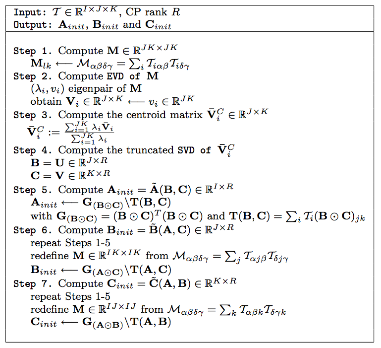
Refer to caption
(a) Centroid Projection Algorithm
Refer to caption
(b) Alternating CP Methods: (ALS, RALS, REALS) with Random Initial Conditions and (CALS, CRALS, CREALS) with Centroid Initial Conditions
Figure 2: CP Methods with Random and Centroid Initial Conditions.

The Centroid Projection method helps mitigate the effects of ALS swamps by providing a good set of initial factors lying close to the true solution subspaces.

5.2 Symmetric CPCP

Refer to caption
Refer to caption
Figure 3: Fully Symmetric CP Decomposition.

The current methods for CP decomposition do not guarantee factorization with identical factors. In fact, when ALS is used in finding tensor decomposition with identical factors, the ALS algorithm will converge to a decomposition with no identical factors. Full and partial symmetries in tensor decomposition are referred to decomposition with at least two factors being identical. In a recent work of Stegeman [22], the existence and uniqueness of the nnth order tensor decompositions with some form of symmetry have been studied for n=3,4,5n=3,4,5. In other works [1, 5], symmetries are also described by the permutation of the multi-indices of the tensor elements. An example is the following: if ti​j​k=tj​k​i=tk​i​jt_{ijk}=t_{jki}=t_{kij}, then 𝒯∈ℝN×N×N\mathcal{T}\in\mathbb{R}^{N\times N\times N} with a tensor rank RR is fully symmetric and its factors are 𝔸=𝔹=ℂ∈ℝN×R\mathbb{A}=\mathbb{B}=\mathbb{C}\in\mathbb{R}^{N\times R}. Another example is if ti​j​k​l=tk​l​i​jt_{ijkl}=t_{klij}, then 𝒯∈ℝM×N×M×N\mathcal{T}\in\mathbb{R}^{M\times N\times M\times N} with a tensor rank RR is partially symmetric and its factors are 𝔸=ℂ∈ℝM×R\mathbb{A}=\mathbb{C}\in\mathbb{R}^{M\times R} and 𝔹=𝔻∈ℝN×R\mathbb{B}=\mathbb{D}\in\mathbb{R}^{N\times R}.

When the Centroid Projection algorithm is applied to the CP methods (CALS, CRALS, CREALS) for symmetric decomposition, the methods with the centroid starters are guaranteed to converge to identical factors provided that the tensor dimensions and order satisfy the uniqueness and existence conditions of Kruskal [13] and Stegeman [22]. In the case that we have fully (partially) symmetric tensor, then I=J=KI=J=K (I=JI=J or J=KJ=K or I=KI=K). Thus, from the EVD of 𝕍¯𝕚∈ℝI×I\mathbb{\mathbb{\bar{V}}_{i}}\in\mathbb{R}^{I\times I}, we obtain the minimizers 𝔹=ℂ\mathbb{B}=\mathbb{C} in Theorem 4.3 .

Figure 3 consists of plots of the number of iterations vs residual errors ‖𝒯o​r​i​g−𝒯e​s​t‖F2\|\mathcal{T}_{orig}-\mathcal{T}_{est}\|_{F}^{2} for symmetric tensor decomposition with identical factors 𝔸=𝔹=ℂ\mathbb{A}=\mathbb{B}=\mathbb{C}. For symmetric CP decomposition, CREALS has outperformed the other iterative methods in Section 5.1 up to a factor of 10410^{4} while ALS has been consistently slow. ALS, RALS and REALS used random initial factors while CALS, CRALS and CREALS used calculated factors via the Centroid Projection algorithm. In most cases, these CPCP methods converged faster than the random-initialized CP methods.

References

  • [1] M. Brazell, N. Li, C. Navasca and C. Tamon. Tensor and Matrix Inversions and Applications, Submitted.
  • [2] J.D. Carroll and J.J. Chang. Analysis of individual differences in multidimensional scaling via an N-way generalization of ‘Eckart-Young’ decomposition, Psychometrika, 35 (1970), pp. 283-319.
  • [3] P. Comon, X. Luciani and A.L.F. de Almeida. Tensor decompositions, altenating least squares and other tales. Journal of Chemometrics, 23 (2009) pp. 393-405.
  • [4] L. De Lathauwer, B. De Moor and J. Vandewalle. On the Best Rank-1 and Rank-(R1,R2,…,RN) Approximation of Higher-Order Tensors, SIMAX 21 4 (2000), pp. 1324–1342.
  • [5] L. De Lathauwer, J. Castaing, and J.-F. Cardoso. Fourth-Order Cumulant-Based Blind Identification of Underdetermined Mixtures. IEEE Transactions on Signal Processing, 55 6 (2007), pp. 2965–2973.
  • [6] V. de Silva and L.-H. Lim. Tensor rank and the ill-posedness of the best low-rank approximation problem. SIAM Journal on Matrix Analysis and Applications, 30 3 (2008), pp. 1084–1127.
  • [7] R.A. Harshman. Foundations of the PARAFAC procedure: Models and conditions for an ”explanatory” multi-modal factor analysis. UCLA working papers in phonetics, 16 (1970), pp. 1–84.
  • [8] A. Hatcher. Algebraic topology. Cambride Universtiy Press, Cambridge (2000).
  • [9] F.L. Hitchcock. The expression of a tensor or a polyadic as a sum of products. Journal of Mathematics and Physics, 6 (1927), pp. 164–189.
  • [10] F.L. Hitchcock. Multilple invariants and generalized rank of a p-way matrix or tensor. Journal of Mathematics and Physics, 7 (1927), pp. 39–79.
  • [11] T. Kolda and B.W. Bader. Tensor decompositions and applications, SIREV, 51 3, (2009), pp. 455–500.
  • [12] W.P. Krijnen, T.K. Dijkstra and A. Stegeman. On the non-existence of optimal solutions and the occurrence of ”degeneracy” in the Candecomp/Parafac model. Psychometrika, 73 (2008) pp. 431–439.
  • [13] J.B. Kruskal. Three-way arrays: rank and uniquenss of trilinear decompositions with applications to arithmetic complexity and statistics, Linear Algebra and its Applications, 18 (1977), pp. 95–138.
  • [14] L. De Lathauwer, B. De Moor, and J. Vandewalle. On the best rank-1 and rank-(R1,R2,…,RN)(R_{1},R_{2},...,R_{N}) approximation of higher-order tensors, SIAM J. Matrix Anal. Appl., 21 (2000), pp. 1324–1342.
  • [15] N. Li, S. Kindermann and C. Navasca. Some convergence results of a regularized alternating least-squares method for tensor decomposition, Submitted.
  • [16] J. Milnor. Morse theory. Princeton University Press, Princton, 1963.
  • [17] C. Navasca, L. De Lathauwer and S. Kindermann. Swamp reducing technique for tensor decomposition, in the 16th Proceedings of the European Signal Processing Conference, Lausanne, August 2008.
  • [18] P. Paatero. The Multilinear Engine - a table-driven least squares program for solving multilinear problems, including the n-way Parallel Factor Analysis model. Journal of Computational and Graphical Statistics, 8 (1999), pp. 854–888.
  • [19] P. Paatero. Construction and analysis of degenerate PARAFAC models. J. Chemometrics, 14 (2000), pp. 285–299.
  • [20] P. Paatero, C. Navasca, and P. Hopke. Fast Rotationally Enhanced Alternating Least-Squares Method, Preprint. http://people.clarkson.edu/∼\simcnavasca/REALS.html
  • [21] M. Rajih and P. Comon. Enhanced line search: A novel method to accelerate Parafac. in the 13th Proceedings of the European Signal Processing Conference, Antalya, Turkey, September 2005.
  • [22] A. Stegeman. On uniqueness of the canonical tensor decomposition with some form of symmetry, to appear in SIMAX.
  • [23] A. Stegeman and L. De Lathauwer. A method to avoid diverging components in the Candecomp/Parafac model for generic I×J×2I\times J\times 2 arrays. SIAM Journal on Matrix Analysis and Applications, 30 (2009) pp. 1614–1638.
  • [24] G. Tomasi and R. Bro. A comparison of algorithms for fitting the PARAFAC model Computational Statistics and Data Analysis, 50 (2006), pp. 1700–1734.