Online Robust Subspace Tracking from Partial Information
Abstract
This paper presents GRASTA (Grassmannian Robust Adaptive Subspace Tracking Algorithm), an efficient and robust online algorithm for tracking subspaces from highly incomplete information. The algorithm uses a robust -norm cost function in order to estimate and track non-stationary subspaces when the streaming data vectors are corrupted with outliers. We apply GRASTA to the problems of robust matrix completion and real-time separation of background from foreground in video. In this second application, we show that GRASTA performs high-quality separation of moving objects from background at exceptional speeds: In one popular benchmark video example [28], GRASTA achieves a rate of 57 frames per second, even when run in MATLAB on a personal laptop.
Keywords: Grassman manifold, Lagrangian alternating direction, subspace tracking, matrix separation, robust PCA, video surveillance.
1 Introduction
Low-rank subspaces have long been a powerful tool in data modeling and analysis. Applications in communications [35], source localization and target tracking in radar and sonar [24], and medical imaging [2] all leverage subspace models in order to recover the signal of interest and reject noise. In these classical signal processing problems, a handful of high-quality sensors are co-located such that data can be reliably collected.
The challenges of modern data analysis breach this standard setup. A first difference, one that cannot be overstated, is that data are being collected everywhere, on a more massive scale than ever before, by cameras, sensors, and people. We give just a few examples: There are an estimated minimum 10,000 surveillance cameras in the city of Chicago and an estimated 500,000 in London [3, 33]. Netflix collects ratings from 25 million users on tens of thousands of movies [13]. On its peak day of the holiday season in 2008, Amazon.com collected data on 72 items purchased every second [44]. The Large Synoptic Survey Telescope, which will be deployed in Chile and will photograph the whole sky visible to it every three nights, will produce 20 terabytes of data every night [39].
A second and equally important difference is that, in all these examples mentioned, the data collected may be unreliable or an indirect indicator of what one really wants to know. The data are collected from many possibly distributed sensors or even from people whose responses may be inconsistent, and the data may be missing or corrupted.
In order to address these issues, algorithms for data analysis must be computationally fast as well as robust to corruption and missing data. In this paper we present the Grassmannian Robust Adaptive Subspace Tracking Algorithm, or GRASTA, an online algorithm for robust subspace tracking that handles these three challenges at once. We seek a low-rank model for data that may be corrupted by outliers and have missing data values.
GRASTA uses the natural -norm cost function for data corrupted by sparse outliers, and performs incremental gradient descent on the Grassmannian, the manifold of all -dimensional subspaces for fixed . For each subspace update, we use the gradient of the augmented Lagrangian function associated to this cost. GRASTA operates only one data vector at a time, making it faster than other state-of-the-art algorithms and amenable to streaming and real-time applications.
1.1 Contributions
The contributions of our work are threefold:
1.1.1 Efficient Grassmannian Augmented Lagrangian Alternating Direction Algorithm
We propose an efficient online robust subspace tracking algorithm – GRASTA, or Grassmannian Robust Adaptive Subspace Tracking Algorithm – which combines the augmented Lagrangian function with the classic stochastic gradient framework [25] and the structure of the Grassmannian [18], and solves via the augmented Lagrangian alternating direction method [7]. As we discuss in detail in Section 2 and 3, GRASTA alternates between estimating a low-dimensional subspace and a triple which represent the sparse corruptions in the signal, the weights for the fit of the signal to the subspace, and the dual vector in the optimization problem. For estimating the subspace , GRASTA uses gradient descent on the Grassmannian with fixed; for estimating the triple , GRASTA uses ADMM [7].
When data vectors arise from an underlying subspace which is inherently low-dimensional, and are corrupted with noise and outliers, GRASTA is able estimate and track the subspace successfully, even when the vectors are highly incomplete.
1.1.2 Fast Robust Low-rank Matrix Completion
We show that GRASTA can successfully recover a low-rank matrix from partial information, even if the partially observed entries are corrupted by gross outliers. GRASTA’s incremental update results in a significant speed-up over other state-of-the-art robust matrix completion algorithms or RPCA (robust principal components analysis) algorithms.
1.1.3 Realtime Separation of Background and Moving Objects in Video Surveillance
Finally, we show that the online nature of GRASTA makes it suitable for realtime high-dimensional sparse signal separation from a background signal, such as the task of separating background and moving objects in video surveillance. Compared to other RPCA methods, GRASTA can handle video frames at very high rates– up to 57 frames per second in our examples– even when implemented in MATLAB on a personal laptop, which is a significant practical advantage over other state-of-the-art techniques.
This paper is organized as follows. We motivate robust online subspace tracking and give background on subspace tracking and matrix completion in Sections 1.2 and 1.3. The familiar reader can go directly to Section 2, where we formulate the robust subspace tracking problem and introduce the novel subspace error function in Section 2. In Section 3, we present the Grassmannian Robust Adaptive Subspace Tracking Algorithm (GRASTA) in detail and discuss critical parts of the implementation; we point out the limitations and merits as compared with other RPCA algorithms. In Section 4, we compare GRASTA with GROUSE and RPCA algorithms via extensive numerical experiments and several real-world video surveillance experiments. Section 5 concludes our work and gives some discussion on future directions.
1.2 Motivations
1.2.1 Online Subspace Tracking within Outliers
GRASTA is built on GROUSE [4], an efficient online subspace tracking algorithm. GROUSE uses an -norm cost function, which is problematic when facing data corruption or noise distributed other than Gaussian.
As an example, we consider using subspaces to detect anomalies in computer networks [26]. A non-robust subspace estimation algorithm like GROUSE would need a special anomaly detection component in order to differentiate anomalies and outliers from the underlying subspace of the traffic data. Often these types of anomaly detection components rely on a lot of parameter tuning and heuristic rules for detection. This motivates a more principled approach that is robust by design: GRASTA.
1.2.2 Robust Principal Component Analysis
Principal Components Analysis [21] is a critical tool for data analysis in many fields. Given a parameter for the number of components desired, PCA seeks to find the best-fit (in an norm sense) -dimensional subspace to data; in other words, it finds the best vectors, the principal components, such that the data can be approximated by a linear combination of those vectors.
The residuals of an -norm error function will be Gaussian distributed. Therefore, even with one outlier data point, the principal components can be arbitrarily far from those without the outlier data point [20]. Modern data applications– such as those in sensor networks, collaborative filtering, video surveillance or the network monitoring example just given– will all experience data failures that result in outliers. Sometimes the outliers are even the signal of interest, as in the case of network anomaly detection or identifying moving objects in the foreground of a surveillance camera.
A good deal of research is therefore focused on Robust PCA, including [14, 11]. Recent work focuses on a problem definition which seeks a low-rank and sparse matrix whose sum is the observed data. The majority of algorithms use SVD (singular value decomposition) computations to perform Robust PCA. The SVD is too slow for many real-time applications, and consequently many online SVD and subspace identification algorithms have been developed, as we discuss in Section 1.3.1. We are therefore motivated to bridge the gap between online algorithms and robust algorithms with GRASTA.
Of course we emphasize that besides the ability to do matrix separation into low-rank and sparse parts, GRASTA can also effectively handle the scenario where the low-rank subspace is dynamic.
1.3 Background
1.3.1 Subspace Tracking
First we briefly describe the subspace tracking problem set-up and GROUSE [4] algorithm before reviewing previous literature on subspace tracking.
Consider a sequence of -dimensional subspaces , , and a sequence of vectors . The object of a subspace tracking algorithm is to estimate , given only and the previous subspace estimate .
Incomplete Data Vectors
Now considering the issue of incomplete data vectors, the object of an algorithm for subspace tracking with missing data is to estimate given – an incomplete version of , observed only on the indices . The GROUSE [4] algorithm addresses exactly this problem. GROUSE is an incremental gradient descent algorithm performed on the Grassmannian , the space of all -dimensional subspaces of . The algorithm minimizes an -norm cost between observed incomplete vectors and their fit to the subspace variable. Each step of the algorithm is simple and requires very few operations. However, the use of the loss makes GROUSE very susceptible to outliers.
Complete Data Vectors
Comon and Golub [15] give an early survey of adaptive methods for tracking subspaces, both coming from the matrix computation literature, including Lanczos-based recursion algorithms, and gradient-based methods from the signal processing literature.
There is a vast literature on the adaptation of QR and SVD factorizations to the adaptive, online context. The work in [6, 34, 43] are all along these lines. The fastest algorithm for incremental SVD is given in [9]; this algorithm makes modifications, one column at a time, to the thin SVD of a strictly rank- matrix in time.
Initial work in signal processing for subspace tracking was aimed at estimating from data the largest eigensubspace for a signal covariance matrix. This is useful, for example, in direction-of-arrival (DOA) estimation: the well-known work in [38] introduces ESPRIT, a parameter estimation algorithm that estimates the DOA of plane waves emanating from a target and being received by a sensor array. ESPRIT was a follow up to the MUSIC algorithm [40], and ESPRIT gains computational efficiency over MUSIC for a slight tradeoff in generality of sensor array design. Around the same time, Yang and Kaveh [47] introduced an approach for subspace tracking that, like GROUSE, uses incremental gradient, thus making it more suitable for adaptive estimation of the signal subspace and covariance matrix. This work was followed by [32, 46, 17] with various improvements and convergence analyses. Unlike GROUSE, these algorithms all conduct gradient descent in the ambient space as opposed to operating along the geodesics of the Grassmannian. Also unlike GROUSE, these algorithms all require fully observed vectors.
Smith [19, 42, 18] thoroughly pursued conjugate gradient descent methods on the Grassmannian for solving the subspace tracking problem using the Rayleigh quotient as a cost function as opposed to the Frobenius norm of GROUSE. In [19] the authors give a very careful definition of the problem, giving a nice survey comparing the applicability of various approaches. In [18] is an extensive list of subspace tracking references.
We note here that none of the work in this subsection addressed issues of robustness to corrupted data or missing data.
Robust Subspace Tracking
The work of [31] addresses the problem of robust online subspace tracking. They focus on the problem where outliers are found in a fraction of vectors (that is, some vectors have no outliers), though they do remark that this can be extended to handle the case where outliers are sparse in every vector. They have a very nice proposition relating -(pseudo)norm minimization to the least trimmed squares estimator.
1.3.2 Matrix Completion
The popular Netflix prize [1] stimulated research on the matrix completion problem: Given very few entries of a low-rank matrix, can one recover (or complete) the entire matrix? When Candès and Recht proved that, under some incoherence conditions, nuclear norm minimization recovers a highly incomplete low rank matrix with high probability [12], an entire area was opened up for further analysis and algorithmic variations. Algorithms that have been proposed to solve matrix completion include ADMiRA [27], OptSpace [22], Singular Value Thresholding [10], FPCA [30], SET [16], APGL [45], GROUSE [4], and many others. Of these, GROUSE is the only online matrix completion algorithm in that it proceeds incrementally, one column at a time. This along with the fact that each update of GROUSE has low computational complexity makes GROUSE the fastest of the state-of-the-art matrix completion algorithms by nearly an order of magnitude [4].
2 Problem Set-up
We denote the evolving -dimensional subspace of as at time . In applications of interest we have . Let the columns of an matrix be orthonormal and span . Tracking the evolving subspace is equivalent to estimating at each time step11 1 We remind the reader here that is not unique for a given subspace, but the projection matrix is unique..
2.1 Model
At each time step , we assume that is generated by the following model:
| (2.1) |
where is the weight vector, is the sparse outlier vector whose nonzero entries may be arbitrarily large, and is the zero-mean Gaussian white noise vector with small variance. We observe only a small subset of entries of , denoted by .
Conforming to the notation of GROUSE [4], we let denote the submatrix of consisting of the rows indexed by ; also for a vector , let denote a vector in whose entries are those of indexed by . A critical problem raised when we only partially observe is how to quantify the subspace error only from the incomplete and corrupted data. GROUSE [4] uses the natural Euclidean distance, the -norm, to measure the subspace error from the subspace spanned by the columns of to the observed vector :
| (2.2) |
It was shown in [5] that this cost function gives an accurate estimate of the same cost function with full data (), as long as is large enough22 2 In [5] the authors show that must be larger than , where is a measure of incoherence on the subspace and controls the probability of the result. See the paper for details.. However, if the observed data vector is corrupted by outliers as in Equation (2.1), an -based best-fit to the subspace can be influenced arbitrarily with just one large outlier; this in turn will lead to an incorrect subspace update in the GROUSE algorithm, as we demonstrate in Section 4.1.
2.2 Subspace Error Quantification by -Norm
In order to quantify the subspace error robustly, we use the -norm as follows:
| (2.3) |
With known (or estimated, but fixed), this minimization problem is the classic least absolute deviations problem; Boyd [7] has a nice survey of algorithms to solve this problem and describes in detail a fast solver based on the technique of ADMM (Alternating Direction Method of Multipliers)33 3 http://www.stanford.edu/~boyd/papers/admm/. More references can be found therein.
According to [7], we can rewrite the right hand of Equation (2.3) as the equivalent constrained problem by introducing a sparse outlier vector :
| (2.4) | |||||
The augmented Lagrangian of this constrained minimization problem is then
| (2.5) |
where is the dual vector. Our unknowns are , , , and . Note that since is constrained to a non-convex manifold (), this function is not convex (neither is Equation (2.2)). However, note that if were estimated, we could solve for the triple using ADMM; also if were estimated, we could refine our estimate of . This is the alternating approach we take with GRASTA. We describe the two parts in detail in Sections 3.1 and 3.2.
2.3 Relation to Robust PCA and Robust Matrix Completion
If the subspace does not evolve over time, this problem reduces to subspace estimation, which can be related to Robust PCA. For a set of time samples , we observe a sequence of incomplete corrupted data vectors . Let the matrix . Let denote operator which selects from each column the corresponding indices in ; thus denotes our partial observation of the corrupted matrix . Note that from our model in Equation (2.1), we can write as a sum of a sparse matrix and a low-rank matrix , where the orthonormal columns of span (which is stationary), and holds the weight vectors as columns.
The global version of the cost function in Equation (2.3) follows:
| (2.6) | |||||
The right hand of Equation (2.6) can be rewritten as the equivalent constrained problem:
| (2.7) | |||||
which is the same problem studied in [41], and the authors propose an efficient ADMM solver for this problem. Unlike the set-up of [14, 11], this problem is not convex; however it offers much more computationally efficient solutions. GRASTA differs from the algorithm of [41] in two major ways: it uses incremental gradient to minimize this cost function one column at a time for even greater efficiency, and it uses geodesics on the Grassmannian to compute the update of .
3 Grassmannian Robust Adaptive Subspace Tracking
As we have said, GRASTA alternates between estimating the triple and the subspace . Here we discuss those two pieces of our algorithm. Section 3.1 describes the update of based on an estimate for the subspace variable. Section 3.2 describes the update of our subspace variable to based on the estimate of resulting from the first step. Finally, Section 3.4 describes our algorithm for adaptively choosing the gradient step-size.
3.1 Update of the sparse vector, weight vector, and dual vector
Given the current estimated subspace , the partial observation , and the observed entries’ indices , the optimal of Equation (2.4) can be found with the following minimization of the augmented Lagrangian.
| (3.1) |
3.2 Subspace Update
As we mentioned in Section 1.3, the set of all subspaces of of fixed dimension is called Grassmannian, which is a compact Riemannian manifold, and is denoted by . Edelman, Arias and Smith (1998) have a comprehensive survey [18] that covers how both the Grassmannian geodesics and the gradient of a function defined on the Grassmannian manifold can be explicitly computed.
GRASTA achieves online robust subspace tracking by performing incremental gradient descent on the Grassmannian step by step. That is, we first compute a gradient of the loss function, and then follow this gradient along a short geodesic curve on the Grassmannian. Figure 1 illustrates the basic idea of gradient descent along a geodesic.

3.2.1 Augmented Lagrangian as the Loss Function
It seems that it would be natural to use Equation (2.3) as the robust loss function. However, there is a critical limitation of this approach: when regarding as the variable, this loss function is not differentiable everywhere.
3.2.2 Grassmannian Geodesic Gradient Step
In order to take a gradient step along the geodesic of the Grassmannian, according to [18], we first need to derive the gradient formula of the real-valued loss function Equation (3.6) .
From Equation (2.70) in [18], the gradient can be determined from the derivative of with respect to the components of . Let is defined to be the columns of an identity matrix corresponding to those indices in ; that is, this matrix zero-pads a vector in to be length with zeros on the complement of . The derivative of the augmented Lagrangian loss function with respect to the components of is as follows:
| (3.7) |
Then the gradient is [18]. Here we introduce three variables , , and to simplify the gradient expression:
| (3.8) | |||||
| (3.9) | |||||
| (3.10) |
Thus the gradient can be further simplified to:
| (3.11) |
From Equation (3.11), it is easy to verify that is rank one since is a vector and is the optimal weight vector. Then it is trivial to compute the singular value decomposition of , which will be used for the following gradient descent step along the geodesic according to Equation (2.65) in [18]. The sole non-zero singular value is , and the corresponding left and right singular vectors are and respectively. Then we can write the SVD of the gradient explicitly by adding the orthonormal set orthogonal to as left singular vectors and the orthonormal set orthogonal to as right singular vectors as follows:
| (3.12) |
Finally, following Equation (2.65) in [18], a gradient step of length in the direction is given by
| (3.13) |
3.3 Remarks
Here we point out that at each subspace update step, our approach does not remove outliers explicitly. In fact, we use the gradient of the augmented Lagrangian Equation (3.6) which exploits the dual vector to leverage the outlier effect. That is the key to success. Even when the ADMM solver 3.2 can not identify the outliers due to our current estimated subspace being far away from the true subspace, with the help of the dual vector the gradient of the augmented Lagrangian gives us the right direction at each step which leads us to the right subspace.
We also must point out that since we estimate at each step using the ADMM solver, we can not recover the exact subspace with sufficient accuracy if we do not allocate enough iterations for the ADMM solver [7]. Fortunately, as it also emphasized in [7], only a few tens of iterations per subspace update step are sufficient to achieve a modest accuracy, which is often acceptable for practical use. Extensive experiments in Section 4 show that our algorithm is fast and always produces acceptable results, even when the vectors are noisy and heavily corrupted by outliers.
3.4 Adaptive Step-size
The question of how large a gradient step to take along the geodesic is an important issue, and it depends on a fundamental tradeoff between tracking rate and steady-state error. Rather than the constant step-size rule proposed for subspace tracking in GROUSE, here we propose to use the adaptive step-size rule to achieve both precise convergence for a stationary subspace and fast adaptation to a changing subspace.
We use the following formula to update the step-size :
| (3.14) |
where is the predefined constant step-size scale. If we use to update , it is obvious that the step-size satisfies the following properties:
This is the classic diminishing step-size rule in stochastic gradient descent literature, and has been proven to guarantee convergence to a stationary point [37] [25].
However, our goal is not only to identify the stationary subspace precisely. We have the more ambitious goal of keeping track of the subspace when the subspace is slowly changing. Obviously, with a changing subspace, if we use a diminishing step-size rule, when is shrinking to our steps will be too small to track the dynamic subspace. To continually adapt to the changing subspace, GROUSE [4] proposes a constant step-size which needs careful selection to balance the tradeoff between tracking rate and steady-state error.
Here we propose to use an adaptive step-size rule to produce a proper step-size that empirically achieves both precise convergence for a stationary subspace and fast adaptation to a changing subspace. The basic idea is inspired by Plakhov [36] and Klein [23]: if two consecutive gradients and are in the same direction, i.e. , it intuitively means that the current estimated is relatively far away from the true subspace . If this is the case, heuristically we should take a slightly larger step along than the previous step-size . Otherwise, if and are not in the same direction, i.e. , again intuitively this means that the current estimated is relatively close the true subspace , and again heuristically we should take a slightly smaller step along than the previous step-size . Besides the sign of the two consecutive gradients giving us intuition for the step-size adaptation, the inner product also gives us the proper adapted magnitude for our step-size [36] [23].
We still use Equation (3.14) to produce at each time, but update according to the inner product of two consecutive gradients as follows:
| (3.15) |
where the function is defined as:
with , , , and . and are chosen to control how much the step-size grows or shrinks; and controls the shape of the function. In this paper we always set , , and .
When the estimated subspace is very close to the true subspace , the adaptive step-size , or equivalently from Equation (3.14). Now we consider the following scenario: suppose we have identified the subspace precisely– and therefore for some large number then suddenly the subspace changes dramatically. How quickly will this step-size rule adapt to the new subspace? In practical applications, taking too much time to adapt to the new subspace is undesirable. Specifically, only shrinking at most is too conservative in this scenario. It is easy to verify that, since at each update step shrinks at most , the increase of is limited and therefore this approach wouldn’t take very large steps even though the subspace has changed. When the subspace changes drastically, we should shrink more to accelerate the adaptation process.
For GRASTA, we take this approach and call it a ”Multi-Level” adaptive step-size rule. Though we do not provide the convergence proof here, empirically this multi-level adaptive approach demonstrates much faster convergence performance than the single-level strategy discussed above. We leave further detailed comparison to future investigation.
Our multi-level adaptation is as follows. We only let change in , where and are prescribed constants. For the experiments in this paper we always set and . Then in this case Equation (3.15) is adapted to Equation (3.16):
| (3.16) |
We introduce a level variable that will get smaller when our subspace estimate is far from the data. Then the step-size is as follows:
| (3.17) |
Once calculated by Equation (3.16) is larger than , we increase the level variable by and set , where and is selected close to (in our experiments we let ). If , we decrease by and also set . Therefore, when our subspace estimate is off, we are increasing exponentially instead of linearly. On one hand this new multi-level adaptive rule follows the basic adaptive step-size rule discussed above; on the other hand exploiting this multi-level property, this new approach adapts more quickly to a changing subspace. Once we have identified the subspace changing and , if the subspace really changes dramatically, will keep decreasing until is again within the range .
Combining these ideas together, we state our novel adaptive step-size rule as Algorithm 3.
3.5 Algorithms
The discussion of Sections 3.1 to 3.4 can be summarized into our algorithm as follows. For each time step , when we observe an incomplete and corrupted data vector , our algorithm will first estimate the optimal value from our current estimated subspace via the minimization ADMM solver 3.2; then compute the gradient of the augmented Lagrangian loss function by Equation (3.11); then estimate a proper step-size from the two consecutive gradients and by Equation (3.15) and 3.17 ; and finally do the rank one subspace update via Equation (3.13).
We state our main algorithm GRASTA (Grassmannian Robust Adaptive Subspace Tracking Algorithm) in Algorithm 1. GRASTA consists of two important sub-procedures: the ADMM solver of the least absolute derivations problem, and the computation of the adaptive step-size. We state the two sub-procedures as Algorithm 2 and Algorithm 3 separately.
Require: An orthogonal matrix . A sequence of corrupted vectors , each vector observed in entries . A structure OPTS1 that holds parameters for ADMM. A structure OPTS2 that holds parameters for the adaptive step size computation.
Return: The estimated subspace at time .
Unlike GROUSE, which has a closed form solution for computing the gradient, GRASTA estimates by the ADMM iterated Algorithm 2. Certainly we would have a potential performance bottleneck if Algorithm 2 takes too much time at each subspace update step. However, we see empirically that only a few tens of iterations in Algorithm 2 at each step allows GRASTA to track the subspace to an acceptable accuracy. In our video experiments with Algorithm 2, we always set the maximum iteration around to balance the trade-off between the subspace tracking accuracy and computational performance. We make a slight modification to the original ADMM sovler presented in [7]: in addition to returning we also return the sparse vector and the dual vector for the further computation of the gradient . It is easy to verify that in the worst case the ADMM solver needs at most flops.
Require: An orthogonal matrix , a corrupted observed vector , and a structure OPTS which holds four parameters for ADMM: ADMM step-size constant , the absolute tolerance , the relative tolerance , and ADMM maximum iteration .
Return: sparse residual ; weight vector ; dual vector .
In order to produce the proper step-size from Algorithm 3, we need to maintain the gradient from the previous time step throughout the subspace tracking process. Keeping only requires additional memory usage. The main computation of of Algorithm 3 is the inner product , which is the trace of the product and , two matrices, and will cost flops.
Require: Previous gradient at time , current gradient at time . Previous step-size variable . Previous level variable . Constant step-size scale . Adaptive step-size parameters .
Return: Current step-size , step-size variable , and level variable .
3.6 Computational Cost and Memory Usage
Each subspace update step in GRASTA needs only simple linear algebraic computations. The total computational cost of each step of Algorithm 1 is , where again is the number of samples per vector used, is the dimension of the subspace, is the ambient dimension, and is the number of ADMM iterations.
Specifically, estimating from Algorithm 2 costs at most flops; computing the gradient needs simple matrix-vector multiplication which costs flops; producing the adaptive step-size costs flops; and the final update step also costs flops.
Throughout the tracking process, GRASTA only needs memory elements to maintain the estimated low-rank orthonormal basis , elements for and , elements for , and for the previous step gradient in memory.
This analysis decidedly shows that GRASTA is both computation and memory efficient.
4 Numerical Experiments
In the following experiments, we explore GRASTA’s performance in various scenarios: subspace tracking, robust matrix completion, and the video surveillance application. We use relative error to quantify the performance of GRASTA. If the recovered data is a vector, the relative error is defined as follows:
| (4.1) |
If the recovered data is a matrix, the relative error is defined as follows:
| (4.2) |
We also use ”Noise Relative Power” to quantify the additional Gaussian white noise perturbation, which is defined as follows:
| (4.3) |
Here is the true data vector and is the additional Gaussian noise as in Equation (2.1).
In all the following experiments, we use Matlab R2010b on a Macbook Pro laptop with 2.3GHz Intel Core i5 CPU and 4 GB RAM. To improve the performance, we implement Algorithm 2 in C++ and make it as a MEX-file to be integrated into GRASTA Matlab scripts.
4.1 Comparison with GROUSE
Our first goal is to compare GRASTA with the non-robust algorithm GROUSE to show the need for a robust subspace estimation and tracking algorithm.
4.1.1 Subspace Tracking with Sparse Outliers
In many of the following experiments, we use this generative model to generate a series of data vectors:
| (4.4) |
is an matrix whose columns are realizations of an i.i.d. random variable that are then orthornomalized. The weight vector is a vector whose entries are realizations of i.i.d. random variables, that is Gaussian distributed with mean zero and variance 1. The sparse vector is an vector whose nonzero entries are Gaussian noise with the maximum of the data vector as the variance; the locations of the nonzero entries are chosen uniformly at random without replacement. The noise is an vector whose entries are i.i.d . This parameter governs the SNR with respect to the low-rank part of our data. For the entire comparison against GROUSE, we used a maximum of iterations of the ADMM algorithm per subspace iteration.
Figure 2 illustrates the failure of GROUSE, and success of GRASTA, when these sparse outliers are added only at periodic time intervals. We can see that GROUSE is significantly thrown off, despite the outliers occurring in an isolated vector. This illustrates clearly our motivation for adding robustness to the subspace tracking algorithm.
4.1.2 Robust Matrix Completion
We aim to complete dimensional matrices of rank . The matrices are corrupted by different fractions of outliers, depending on the experimental setting, and sampled uniformly without replacement with density . We generate the low-rank matrix by first generating two factors and with i.i.d. Gaussian entries and then adding normally distributed noise with variance . The location of sparse outliers is distributed uniformly, and the outlier values are normally distributed with variance equal to the maximum of the matrix.
For each setting of the fraction of outliers, we randomly generate matrices, each of which is solved via GROUSE and GRASTA separately. Both GROUSE and GRASTA cycle through the matrix columns times. Table 1 shows the averaged results of a comparison between GROUSE and GRASTA. As expected, GRASTA vastly outperforms GROUSE across the board even with the smallest number of outliers.
| Fraction of Outliers | ||||||
|---|---|---|---|---|---|---|
| 0 | 0.01 | 0.05 | 0.10 | 0.15 | 0.20 | |
| GROUSE | 3.17E-6 | 3.95E-1 | 5.04E-1 | 8.27E-1 | 8.79E-1 | 9.35E-1 |
| GRASTA | 7.25E-6 | 8.92E-5 | 1.13E-4 | 2.14E-4 | 2.91E-4 | 4.41E-4 |
4.2 Stationary Subspace Identification
Now we wish to examine GRASTA’s performance on the stationary subspace identification problem under various conditions. In most experiments (and unless otherwise noted) the ambient dimension is and the inherent subspace dimension is . We again generate the vectors using Equation (4.4) above and the descriptive text that follows Equation (4.4). We vary the fraction of entries that are corrupted, and we vary the fraction of entries that are observed.
We start with Figure 3, which shows subspace estimation performance under a varying fraction of added outliers. We can see in this problem instance that with 10% corrupted entries, the relative error reaches the relative noise floor after a number of iterations that is a small multiple of the ambient dimension. For more corruption, more vectors (gradient iterations) are needed, but even with 50% outliers and more, the relative error trends toward the relative noise power.
In Figure 4, we consider GRASTA’s error performance for varying sub-sampling rates. Here the fraction of corrupted values is fixed at 10%. We can see that again, even with a 30% sampling rate, the relative error quickly reaches the relative noise power.
Now we wish to take a closer look at the case when we have both dense outlier corruption and subsampling of the signal. This is an important scenario for applications where the “outlier corruption” is a signal of interest obscuring a low-rank background signal, and we wish to subsample in order to improve computational complexity. For example this would apply to anomaly detection problems or to the problem of separation of background and moving objects in video as we show in Section 4.5.
Figure 5 illustrates that even when the vector is highly corrupted with 50% added outliers, GRASTA can identify the underlying low-rank subspace even with only 50% of the entries. We vary the dimension (or rank) of the underlying subspace, and because of this there is not one relative noise power benchmark to compare against; however we see that the trend is similar to those in previous figures.
4.3 Dynamic Subspace Tracking
The fact that GRASTA operates one vector at a time allows it to track an evolving subspace. In this section we show GRASTA’s performance under two models of evolving subspaces. In these experiments, we use the same set-up as before: , , and is generated by Equation (4.4), except that , i.e. the subspace we wish to estimate varies with time :
| (4.5) |
4.3.1 Rotating Subspace Tracking
We use the following ordinary differential equation to simulate a rotating subspace:
| (4.6) |
where is a skew-symmetric matrix. Consequently, the subspace is updated via
where controls the amount of rotation of with each time step . As we see in Figure 6, for the rotation parameter fixed at , GRASTA successfully latches on and tracks the rotating subspace.
4.3.2 Sudden Subspace Change Tracking
For this experiment, we wanted to see the behavior of GRASTA when the subspace experienced a sudden dramatic change. At intervals of 5000 vectors, we randomly changed the true subspace to a new random subspace. The results are in Figure 7. Again from these simulations we see that GRASTA successfully identifies the subspace change and tracks the subspace again.
4.4 Comparison with Robust PCA
Here we compare GRASTA with RPCA on the recovery of corrupted low-rank matrices. For RPCA we use [29], or the IALM (Inexact Augmented Lagrange Multiplier) method44 4 The code we used is available here: http://perception.csl.uiuc.edu/matrix-rank/sample_code.html. We downloaded it in April 2011..
The corrupted matrices can be written as , where are the low-rank matrices we want to recover, are the sparse outlier matrices, and are the Gaussian noise matrices with small variance relative to the sparse outliers. We use matrices of size to do the comparison. The low-rank matrices are generated by the same method of the previous robust matrix completion experiments: as the product of two factors and with i.i.d. Gaussian entries. The sparse outlier matrices are generated by selecting a fraction of entries uniformly at random without replacement, whose values are set according to Gaussian distribution with the maximum of as the variance55 5 We note here that in [29], the authors use a uniform distribution for the outliers, as opposed to Gaussian. The authors in [11] use Bernoulli variables. Gaussian is the most challenging case, because more outliers will be near zero and confuse the estimation.. We vary the fraction of corruptions from (sparse outliers) to (dense outliers), and we also vary the variance Gaussian noise matrices from a moderate perturbation of to a larger perturbation of . For GRASTA we cycled through the matrix columns twice and used a maximum of iterations of the ADMM algorithm; we used a maximum of iterations of IALM.
Table 2 shows the results of the comparison. We ran RPCA with full data, GRASTA with full data, and then GRASTA with various levels of subsampling. When there are very few outliers and little noise, RPCA achieves a reasonable error rate at computational speeds similar to GRASTA. However with an increase in noise or fraction of outliers, GRASTA achieves good error performance in much less time. As a particular example, when and the fraction of outliers is 30%, in 69 seconds GRASTA with full data achieves better error performance than RPCA in 363 seconds, and GRASTA with 30% subsampling achieves better error performance in only 23 seconds.
| GRASTA | GRASTA | GRASTA | IALM | ||
| 1.38 E-4 / 56.62 sec | 2.03 E-4 / 30.46 sec | 2.73 E-4 / 20.51 sec | 5.80 E-5 / 35.26 sec | ||
| 3.64 E-4 / 58.31 sec | 4.65 E-4 / 31.23 sec | 6.07 E-4 / 20.79 sec | 1.67 E-3 / 93.16 sec | ||
| 7.64 E-4 / 59.55 sec | 9.59 E-4 / 31.81 sec | 1.23 E-3 / 20.66 sec | 3.64 E-3 / 117.76 sec | ||
| 4.65 E-4 / 67.90 sec | 7.28 E-4 / 35.10 sec | 1.06 E-3 / 22.96 sec | 1.80 E-4 / 232.26 sec | ||
| 6.13 E-4 / 67.19 sec | 9.08 E-4 / 34.53 sec | 1.26 E-3 / 22.63 sec | 2.64 E-3 / 324.26 sec | ||
| 9.87 E-4 / 69.06 sec | 1.44 E-3 / 35.61 sec | 1.93 E-3 / 22.85 sec | 5.62 E-3 / 362.62 sec | ||
| 1.26 E-3 / 83.11 sec | 2.05 E-3 / 39.90 sec | 3.58 E-3 / 25.33 sec | 1.43 E-1 / 341.01 sec | ||
| 1.33 E-3 / 81.51 sec | 2.24 E-3 / 40.33 sec | 3.93 E-3 / 25.38 sec | 1.45 E-1 / 351.26 sec | ||
| 1.64 E-3 / 82.23 sec | 2.85 E-3 / 41.91 sec | 5.08 E-3 / 25.67 sec | 1.62 E-1 / 372.21 sec | ||
4.5 Realtime Video Background Tracking and Foreground Detection
In this subsection we discuss the application of GRASTA to the prominent problem of realtime separation of foreground objects from the background in video surveillance. Imagine we had a video with only the background: When the columns of a single frame of this video are stacked into a single column, several frames together will lie in a low-dimensional subspace. In fact if the background is completely static, the subspace would be one-dimensional. That subspace can be estimated in order to identify and separate the foreground objects; if the background is dynamic, subspace tracking is necessary. GRASTA is uniquely suited for this burgeoning application.
Here we consider three scenarios in the video tasks, with a spectrum of challenges for subspace tracking. In the first we have a video with a static background and objects moving in the foreground. In the second, we have a video with a still background but with changing lighting. In the third, we simulate a panning camera to examine GRASTA’s performance with a dynamic background. The results are summarized in Table 3.
4.5.1 Static Background
If the video background is known to be static or near static, we can use GRASTA to track the background and separate the moving foreground objects in real-time. Since the background is static, we use GRASTA first to identify the background, and then we use only Algorithm 2 to separate the foreground from the background. More precisely we do the following:
- 1.
Randomly select a few frames of the video to train the static low-rank subspace . In our experiments, we select frames randomly from the entire video; however for real-time processing these frames may be chosen from initial piece of the video, as long as we can be confident that every pixel of the background is visible in one of the selected frames. The low-rank subspace is then identified from these frames using partial information. We use of the pixels, select frames for training, and set RANK = 5 in all the following experiments.
- 2.
Once the video background has been identified as a subspace , separating the foreground objects from each frame can be simply done using Equation (4.7), where the weight vector can be solved for via Algorithm 2, again from a small subsample of each frame’s pixels.
(4.7)
Table 3 shows the real-time66 6 We comment here that to call something “real-time” processing of course will depend on one’s application requirements and hardware (camera frame capture rate, in the example of video processing). For example, standard 35mm film video uses 24 unique frames per second. The maximum frame rate for most CCTVs is 30 frames per second. video separation results. From the first experiment, we use the “Hall” dataset from [28] which consists of frames each with resolution . We let GRASTA cycle times over the training frames just from random entries of each frame to get the stationary subspace . Training the subspace costs seconds. Then we perform background and foreground separation for all frames in a streaming fashion, and when dealing with each frame we only randomly observe entries. The separation task is performed by Equation (4.7), and the separating time is seconds, which means we achieve FPS (frames per second) real-time performance. Figure 8 shows the separation quality at . In order to show GRASTA can handle higher resolution video effectively, we use the “Shopping Mall” [28] video with resolution as the second experiment. We also do the subspace training stage with the same parameter settings as “Hall”. We do the background and foreground separation only from entries of each frame. For “Shopping Mall” the separating time is seconds for total frames. Thus we achieve FPS real-time performance. Figure 9 shows the separation quality at . In all of these video experiments we used a maximum of iterations of the ADMM algorithm per subspace update. The details of each tracking set-up are described in Table 4.
| Dataset | Resolution | Total Frames | Training Time | Tracking and | FPS |
|---|---|---|---|---|---|
| Separating Time | |||||
| Hall | 144176 | 3584 | 6.9 sec | 62.5 sec | 57.3 |
| Shopping Mall | 320256 | 1286 | 23.2 sec | 39.1 sec | 32.9 |
| Lobby | 144176 | 1546 | 3.9 sec | 71.3 sec | 21.7 |
| Hall with Virtual Pan (1) | 14488 | 3584 | 3.8 sec | 191.3 sec | 18.7 |
| Hall with Virtual Pan (2) | 14488 | 3584 | 3.7 sec | 144.8 sec | 24.8 |
| Dataset | Training | Tracking | Separation | Training Algorithm | Tracking/Separation Algorithm |
|---|---|---|---|---|---|
| Sub-Sampling | Sub-Sampling | Sub-Sampling | |||
| Hall | 30% | - | 5% | Full GRASTA Alg 1 | Alg 2+Eqn 4.7 |
| Shopping Mall | 30% | - | 1% | Full GRASTA Alg 1 | Alg 2+Eqn 4.7 |
| Lobby | 30% | 30% | 100% | Full GRASTA Alg 1 | Full GRASTA Alg 1 |
| Hall with Virtual Pan (1) | 100% | 100% | 100% | Full GRASTA Alg 1 | Full GRASTA Alg 1 |
| Hall with Virtual Pan (2) | 50% | 50% | 100% | Full GRASTA Alg 1 | Full GRASTA Alg 1 |


4.5.2 Dynamic Background: Changing Lighting
Here we want to consider a problem where the lighting in the video is changing throughout. We use the “Lobby” dataset from [28], which has frames, each pixels. In order to adjust to the lighting changes, GRASTA tracks the subspace throughout the video; that is, unlike the last two experiments, we run the full GRASTA Algorithm 1 for every frame. We use 30% of the pixels of every frame to do this update and 100% of the pixels to do the separation. Again, see the numerical results in Table 3. The results are illustrated in Figure 10.

4.5.3 Dynamic Background: Virtual Pan
In the last experiment, we demonstrate that GRASTA can effectively track the right subspace in video with a dynamic background. We consider panning a ”virtual camera” from left to right and right to left through the video to simulate a dynamic background. Periodically, the virtual camera pans 20 pixels. The idea of the virtual camera is illustrated cleanly with Figure 11.
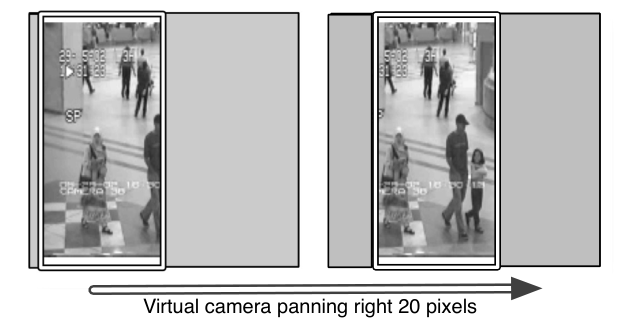
We choose “Hall” as the original dataset. The original resolution is , and we set the scope of the virtual camera to have the same height but half the width, so the resolution of the virtual camera is . We set the subspace . Figure 12 shows how GRASTA can quickly adapt to the changed background in just frames when the virtual camera pans pixels to the right at . We also let GRASTA track all the frames and do the separation task for all frames. When we use 100% of the pixels for the tracking and separation, the total computation time is seconds, or FPS, and adjusting to a new camera position after the camera pans takes frames as can be seen in Figure 12. When we use 50% of the pixels for tracking and 100% of the pixels for separation, the total computation time is seconds or FPS, and the adjustment to the new camera position takes around 50 frames.

5 Discussion and Future Work
In this paper we have presented a robust online subspace tracking algorithm, GRASTA. The algorithm estimates a low-rank model from noisy, corrupted, and incomplete data, even when the best low-rank model may be changing over time.
Though this work presents some very successful algorithms, many questions remain. First and foremost, because the cost function in Equation (2.3) has the subspace variable which is constrained to a non-convex manifold, the resulting optimization is non-convex. A proof of convergence to the global minimum of this algorithm is of great interest.
GRASTA uses alternating minimization, alternating first to estimate and then fixing this triple of variables to estimate . Observe that if are correct estimates, we could then estimate without the robust cost function. This would be quite useful in situations when speed is of utmost importance, as the GROUSE subspace update is faster than the GRASTA subspace update. Of course, knowing when are accurate is a very tricky business. Exploring this tradeoff is part of our future work.
We have shown that one of the very promising applications of GRASTA is that of separating background and foreground in video surveillance. We are very interested to apply GRASTA to more videos with dynamic backgrounds: for example, natural background scenery which may blow in the wind. In doing this we will study the resulting trade-off between the kinds of movement that would be captured as part of the background and the movement that would be identified as foreground.
Acknowledgments
The authors would like to thank IPAM, the Institute for Pure and Applied Mathematics, and the Internet Multi-Resolution Analysis program, which brought them together to work on this problem. We also thank Rob Nowak and Ben Recht for their thoughtful suggestions.
References
- [1] ACM SIGKDD and Netflix. Proceedings of KDD Cup and Workshop, 2007. Proceedings available online at http://www.cs.uic.edu/~liub/KDD-cup-2007/proceedings.html.
- [2] Michel A. Audette, Frank P. Ferrie, and Terry M. Peters. An algorithmic overview of surface registration techniques for medical imaging. Medical Image Analysis, 4(3):201 – 217, 2000.
- [3] Don Babwin. Cameras make chicago most closely watched U.S. city. Huffington Post, April 6 2010. Available at http://www.huffingtonpost.com/2010/04/06/cameras-make-chicago-most_n_527013.html.
- [4] Laura Balzano, Robert Nowak, and Benjamin Recht. Online identification and tracking of subspaces from highly incomplete information. In Proceedings of Allerton, September 2010. Available at http://arxiv.org/abs/1006.4046.
- [5] Laura Balzano, Benjamin Recht, and Robert Nowak. High-dimensional matched subspace detection when data are missing. In Proceedings of ISIT, 2010.
- [6] Christian H. Bischof and Gautam M. Scroff. On updating signal subspaces. IEEE Transactions on Signal Processing, 40(1), January 1992.
- [7] S. Boyd, N. Parikh, E. Chu, B. Peleato, and J. Eckstein. Distributed optimization and statistical learning via the alternating direction method of multipliers. Foundations and Trends in Machine Learning, 3(1):1–123, 2011.
- [8] S.P. Boyd and L. Vandenberghe. Convex optimization. Cambridge Univ Pr, 2004.
- [9] M Brand. Fast low-rank modifications of the thin singular value decomposition. Linear Algebra and its Applications, 415(1):20–30, 2006.
- [10] Jian-Feng Cai, Emmanuel J. Candès, and Zuowei Shen. A singular value thresholding algorithm for matrix completion. SIAM Journal on Optimization, 20(4):1956–1982, 2008.
- [11] E. J. Candès, X. Li, Y. Ma, and J. Wright. Robust principal component analysis? Journal of the ACM, 58(1):1–37, 2009.
- [12] Emmanuel Candès and Benjamin Recht. Exact matrix completion via convex optimization. Foundations of Computational Mathematics, 9(6):717–772, 2009.
- [13] Netflix Media Center. Accessed August 2011 at http://www.netflix.com/MediaCenter.
- [14] V. Chandrasekaran, S. Sanghavi, P.A. Parrilo, and A.S. Willsky. Rank-sparsity incoherence for matrix decomposition. SIAM Journal on Optimization, 21:572, 2011.
- [15] Pierre Comon and Gene Golub. Tracking a few extreme singular values and vectors in signal processing. Proceedings of the IEEE, 78(8), August 1990.
- [16] Wei Dai, Olgica Milenkovic, and Ely Kerman. Subspace evolution and transfer (set) for low-rank matrix completion. IEEE Transactions on Signal Processing, 59(7):3120–3132, 2011.
- [17] J.-P. Delmas and J.-F. Cardoso. Performance analysis of an adaptive algorithm for tracking dominant subspaces. Signal Processing, IEEE Transactions on, 46(11):3045 –3057, nov 1998.
- [18] Alan Edelman, Tomas A. Arias, and Steven T. Smith. The geometry of algorithms with orthogonality constraints. SIAM Journal on Matrix Analysis and Applications, 20(2):303–353, 1998.
- [19] Alan Edelman and Steven T. Smith. On conjugate gradient-like methods for eigen-like problems. BIT Numerical Mathematics, 36:494–508, 1996. 10.1007/BF01731929.
- [20] Peter J. Huber and Elvezio M. Ronchetti. Robust Statistics. Wiley, 2009.
- [21] I. Jolliffe. Principal Component Analysis. Springer-Verlag, 1986.
- [22] R.H. Keshavan, A. Montanari, and S. Oh. Matrix completion from noisy entries. Journal of Machine Learning Research, 11:2057–2078, July 2010.
- [23] S. Klein, J.P.W. Pluim, M. Staring, and M.A. Viergever. Adaptive stochastic gradient descent optimisation for image registration. International journal of computer vision, 81(3):227–239, 2009.
- [24] H. Krim and M. Viberg. Two decades of array signal processing research: the parametric approach. Signal Processing Magazine, IEEE, 13(4):67–94, July 1996.
- [25] H.J. Kushner and G. Yin. Stochastic approximation and recursive algorithms and applications, volume 35. Springer Verlag, 2003.
- [26] Anukool Lakhina, Mark Crovella, and Christophe Diot. Diagnosing network-wide traffic anomalies. In Proceedings of SIGCOMM, 2004.
- [27] Kiryung Lee and Yoram Bresler. Efficient and guaranteed rank minimization by atomic decomposition. In IEEE International Symposium on Information Theory, 2009.
- [28] Liyuan Li, Weimin Huang, Ireme Yu-Hua Gu, and Qi Tian. Statistical modeling of complex background for foreground object detection. IEEE Transactions on Image Processing, 13(11):1459–1472, November 2004.
- [29] Z. Lin, M. Chen, L. Wu, and Y. Ma. The augmented lagrange multiplier method for exact recovery of corrupted low-rank matrices. Arxiv preprint arXiv:1009.5055, 2010.
- [30] Shiqian Ma, Donald Goldfarb, and Lifeng Chen. Fixed point and bregman iterative methods for matrix rank minimization. Mathematical Programming, 128:321–353, 2011. 10.1007/s10107-009-0306-5.
- [31] Gonzalo Mateos and Georgios B. Giannakis. Sparsity control for robust principal component analysis. In Proceedings of 44th Asilomar Conference on Signals, Systems, and Computers, Pacific Grove, CA, November 2010.
- [32] G Mathew, Vellenki Reddy, and Soura Dasgupta. Adaptive estimation of eigensubspace. IEEE Transactions on Signal Processing, 43(2), February 1995.
- [33] Michael McCahill and Clive Norris. Cctv in london. Working Paper 6, Centre for Criminology and Criminal Justice, University of Hull, United Kingdom, June 2002. Available at http://www.urbaneye.net/results/ue_wp6.pdfSimilar.
- [34] Marc Moonen, Paul Van Dooren, and Joos Vandewalle. An SVD updating algorithm for subspace tracking. IEEE Transactions on Signal Processing, 40(6):1535–1541, June 1992.
- [35] E. Moulines, P. Duhamel, J.-F. Cardoso, and S. Mayrargue. Subspace methods for the blind identification of multichannel fir filters. Signal Processing, IEEE Transactions on, 43(2):516–525, feb 1995.
- [36] A. Plakhov and P. Cruz. A stochastic approximation algorithm with step-size adaptation. Journal of Mathematical Sciences, 120(1):964–973, 2004.
- [37] H. Robbins and S. Monro. A stochastic approximation method. The Annals of Mathematical Statistics, pages 400–407, 1951.
- [38] R Roy and T Kailath. ESPRIT – estimation of signal parameters via rotational invariance techniques. IEEE Transactions on Acoustics, Speech, and Signal Processing, 37(7):984–995, July 1989.
- [39] Andrew Schechtman-Rook. Personal Communication, 2011. Details at http://www.lsst.org/lsst/science/concept_data.
- [40] Ralph O. Schmidt. Multiple emitter location and signal parameter estimation. IEEE Transactions on Antennas and Propagation, AP-34(3):276–280, March 1986.
- [41] Y. Shen, Z. Wen, and Y. Zhang. Augmented lagrangian alternating direction method for matrix separation based on low-rank factorization. TR11-02, Rice University, 2011.
- [42] Steven T. Smith. Geometric Optimization Methods for Adaptive Filtering. PhD thesis, Harvard University, 1993.
- [43] G. W. Stewart. An updating algorithm for subspace tracking. IEEE Transactions on Signal Processing, 1992.
- [44] Tess Stynes. Amazon lauds its holiday sales. Wall Street Journal, January 15 2009. Available at http://online.wsj.com/article/SB123029910235635355.html.
- [45] Kim-Chuan Toh and Sangwoon Yun. An accelerated proximal gradient algorithm for nuclear norm regularized linear least squares problems. Pacific Journal of Optimization, 6(3):615–640, 2010.
- [46] Bin Yang. Projection approximation subspace tracking. IEEE Transactions on Signal Processing, 43(1), January 1995.
- [47] Jar-Ferr Yang and Mostafa Kaveh. Adaptive eigensubspace algorithms for direction or frequency estimation and tracking. IEEE Transactions on Acoustics, Speech, and Signal Processing, 36(2), February 1988.