CERN-TH-2011-202
MCNET-11-22
Efficient Matrix-Element Matching with Sector Showers
J.J. Lopez-Villarejo and P. Skands
Theoretical Physics, CERN CH-1211,
Geneva 23, Switzerland
Abstract — A Markovian shower algorithm based on “sector antennae” is presented and its main properties illustrated. Tree-level full-color matrix elements can be automatically incorporated in the algorithm and are re-interpreted as process-dependent antenna functions. In hard parts of phase-space, these functions generate tree-level matrix-element corrections to the shower. In soft parts, they should improve the logarithmic accuracy of it. The number of matrix-element evaluations required per order of matching is 1, with an unweighting efficiency that remains very high for arbitrary numbers of legs. Total rates can be augmented to NLO precision in a straightforward way. As a proof of concept, we present an implementation in the publicly available Vincia plug-in to the Pythia 8 event generator, for hadronic decays including tree-level matrix elements through .
1 Introduction
Perturbative calculations of high-energy processes typically start from the calculation of one or more Matrix Elements (MEs) for specific signal and background processes. By virtue of the factorization theorem, such “hard” or “short-distance” partonic processes can be factored off from lower-scale physics and computed in a systematic way. At Leading Order (LO), the procedure is standard textbook material and it has also by now been highly automated, by the advent of general-purpose tools like CalcHep [1], CompHep [2], MadGraph [3], and others [4, 5, 6, 7, 8].
To the simple LO picture, several corrections must be added in order to obtain more realistic and accurate descriptions that can be compared with experimental observables. On the perturbative side, one may access these corrections either by computing more coefficients in the fixed-order expansion explicitly — as in higher-order calculations — or by approximating them via infinite-order resummations — as in parton showers.
To help illustrate the complementarity of these two approaches, for an arbitrary final state, “”, we shall use diagrams such as the ones shown in fig. 1, from [9], in which the horizontal and vertical axes indicate the numbers of additional legs and loops beyond LO, respectively.
| F @ LO | ||||||||||||||||||||||||||||
|
| F @ NLO | ||||||||||||||||||||||||||||
|
| F @ LOLL | ||||||||||||||||||||||||||||
|
The notation is used to represent the sum of contributions to the cross section for fixed and . These are separately divergent for , and only the sum over all coefficients with fixed is finite. (See [9] for a more pedagogical introduction to this type of diagrams.)
In the left-hand pane of fig. 1, the part of the series covered by the LO matrix element has been shaded. In a Next-to-Leading-Order (NLO) calculation, two further coefficients are computed exactly, as illustrated in the middle pane, but all other coefficients are neglected. Conversely, in a Leading-Logarithmic (LL) resummation, infinite numbers of both legs and loops can be included, but only the leading singular parts of each coefficient will be correctly accounted for, which we illustrate by giving the boxes corresponding to coefficients with a lighter (yellow) shading in the right-hand pane of fig. 1.
Several approaches for “matching” the two kinds of approaches are already in widespread use. Here, we shall focus on the matching of parton showers to LO matrix elements with large numbers of additional legs. For this problem, there are essentially two dominant approaches, called MLM (see [10] for a description) and (L)-CKKW [11, 12, 13, 14, 15], see [16] for a recent pedagogical review. Two main limiting factors in these approaches are that the computational speed falls off steeply with the number of matched partons, and that both approaches only apply matching above a certain “matching scale”, below which the pure shower is used for all multiplicities. This is illustrated in fig. 2a, in which the matched multiplicities are shown with half light (yellow) and half dark (green) shading.
| F @ LOLL | ||||||||||||||||||||||||||||
|
| F @ NLO+LOLL | ||||||||||||||||||||||||||||
|
An alternative multileg matching strategy was recently proposed by GKS [17]. This algorithm uses an antenna-based parton shower [18, 19] as its underlying phase-space generator11 1 The idea of using a shower for phase-space generation also underlies the SARGE [20] and GENEVA [21] algorithms.. Matching to matrix elements is performed by applying multiplicative corrections to the branching probability at each step of the algorithm, an approach that was first pioneered in [22] for matching to a single additional parton in PYTHIA [23]. The generalization to multiple legs proposed in [17] relies explicitly on unitarity to remove the need for a matching scale also beyond the first matched leg. In principle, it can therefore be applied over all of phase-space up to the highest matched multiplicity, though for reasons of algorithmic speed, a low matching scale may still be imposed beyond the first few additional legs. The part of the perturbative series that can be covered by this approach is illustrated in fig. 2b. We note that the one-loop correction to the lowest multiplicity can also be included (as indicated on the figure), since the GKS formalism essentially reduces to the POWHEG one [24, 25] at this order.
In terms of algorithmic speed, the number of individual shower paths that populate each -parton phase-space point is a deciding factor within the GKS formalism, since at least one -parton matrix element has to be evaluated for each path. Showers based on partons and/or partitioned dipoles (such as Altarelli-Parisi [26, 27, 28, 29] or Catani-Seymour [30, 31, 32, 33] ones) produce one term per color charge in the event, i.e., one per quark and two per gluon. Showers based on antennae [34, 35, 36, 18] are slightly more economic, producing only one term per color-connected pair of color charges. This difference is still comparatively insignificant, however, compared to the proliferation of terms caused by the fact that only strongly ordered paths can contribute (using whatever definition of ordering the particular shower algorithm’s authors prefer): to see which paths actually contribute to each -parton configuration, one must check the ordering condition all the way back to the Born configuration, including the effects of any previous matching steps. Even for the antenna-based showers, this makes the number of paths contributing to the branching grow like , which quickly becomes intractable. The main improvement proposed in [17] was to replace the strong-ordering condition by a smoothly damped and strictly Markovian equivalent, which eliminates the factorial. This brings the number of terms produced at each order down to a linear dependence on , resulting in substantial speed gains for high parton multiplicities.
There is, however, an alternative formulation of the antenna language [37, 38], for which only one term contributes to each phase-space point. We refer to this as “sector” antennae, to distinguish them from the “global” antennae used in [39, 17]. The two kinds differ in how the collinear singularities of gluons are partitioned among neighboring antennae. In the global approach, the gluon-collinear singularity is partitioned such that two neigbouring antennae each contain “half” of it; their sum reproduces the full singularity. In the sector case, both of the neighboring antennae contain the full collinear singularity, but only one of them (typically the most singular one) is allowed to contribute to each -parton phase-space point. This divides up the -parton phase-space into a number of “sectors” inside each of which only a single antenna contributes.
In this paper, we present a complete shower formalism based on such sector antennae, including an adaptation and implementation of GKS matching. We note that another formalism dealing with sector showers has also been proposed [40, 41]. While those works also treat polarization and mass effects, which are neglected here, they do not contain an explicit implementation or matching strategy, which are included here and have been made publicly available in the VINCIA code [42], a plug-in to the PYTHIA 8 event generator [43], starting from VINCIA version 1.0.26.
In section 2, we briefly summarize some convenient notation choices we shall use in the remainder of the paper. In section 3, we present the sector antenna functions that have been implemented in VINCIA, including a discussion of their ambiguous non-singular terms and the choice of sector decomposition criterion. Some comparisons to higher-multiplicity tree-level matrix elements are also given, to investigate how the quality of the approximation evolves with parton multiplicity. In section 4, we adapt the VINCIA shower formalism to sector antennae, including trial branchings and GKS matching. Section 5 contains some basic validation comparisons, to show that the implementation gives sensible results. We also present a speed comparison between various different matching strategies, quantifying the improvement obtained for the GKS matching in the sector case. Finally, in section 6, we round off with conclusions and an outlook.
2 Conventions
Dipole-antenna showers [34, 35, 36, 18] are based on nested splitting processes, with an on-shell, Lorentz-invariant phase-space factorization taking place at each step [37, 38]. Following [39, 17], we label the participants in a dipole-antenna branching by . By energy-momentum conservation we have . We denote the dimensionless (scaled) post-branching invariants by
| (1) |
and we define the of a splitting process in the same way as in Ariadne [35],
| (2) |
Contours of constant value of (normalized so that its maximal value is unity) are illustrated in the left-hand pane of fig. 3. For comparison, contours of constant , which we shall use for processes involving splittings below, are illustrated in the right-hand pane of the figure.
For the antenna functions, we shall use the following general notation, which is intended to be analogous to that used for parton distribution functions (PDFs), for the emission of a parton of type j from a parent dipole of type IK,
| (3) |
where “type(order)” specifies the type (sector or global) and loop order of the function, and the arguments , , and represent the final-state momenta of the corresponding color-ordered post-branching particles. As is the case for PDFs, one or more of the super- and subscripts can be omitted when they are obvious from context. This results in a fully general but nevertheless quite compact notation, which we summarize in tab. 1, including a comparison to the notation used for global antennae in [39].
Part of the motivation for introducing this notation, apart from the desire to be able to distinguish clearly between sector and global functions when necessary, is that it generalizes easily to include more branching types, such as ones involving photons in QED, and to higher-order antenna functions, such as ones. We also note that, e.g., , by charge conjugation, with the appropriate permutation of invariants ().
The antenna functions have dimension GeV-2. It is often convenient to work with a color- and coupling-stripped variant, which we label , defined by
| (4) |
where and is the color factor assigned to the branching, defined in the normalization convention of [17], such that, in the leading-color limit, and .
When comparing to collinear (Altarelli-Parisi) splitting functions [26], we define as the momentum fraction of the radiated parton in the collinear limit:
| (5) | |||||
| (6) |
The AP splitting functions for and are then
| (7) | |||||
| (8) |
which we shall use when analyzing the collinear singular limits of the corresponding global and sector antenna functions below.
3 The Sector Antennae
In the sector approach, only one antenna contributes to any given phase-space point, as opposed to several overlapping ones in the global antenna case. The three different phase-space sectors that occur for (with cyclic color connections, as in ) are illustrated in fig. 4 [17].
In a global shower, the antenna, shown in the left-hand pane, would be allowed to fill the entire branching phase-space, which is defined by the triangle . In the sector case, however, it only fills the part of phase-space in which the transverse momentum of with respect to and is smaller than that of either of the two other possible combinations (assuming transverse momentum is what is used to separate the sectors, a point we return to below). The remaining part of phase-space is not empty — it is filled by the two complementary permutations of the , , and partons, as shown in the middle and right-hand panes of the figure. The coefficients of the singular terms of the antenna functions must necessarily reflect this reorganization. The double pole, located at the origin of the plots in fig. 4, is contained entirely within the antenna, and can therefore be carried over from the global case without modification. The single-pole terms, however, change to account for collinear radiation now being produced by a single antenna rather than two overlapping ones.
In section 3.1, we discuss how the singularity structure of the individual antennae is modified and derive a complete set of sector antenna functions. In section 3.2, we compare these functions to fixed-order matrix elements for , , and partons. In section 3.3, we discuss the ambiguities remaining concerning non-singular (and non-universal) terms. Finally, in section 3.4, we compare various options for how to partition phase-space into sectors.
3.1 Singularity Structure
In the so-called “planar” (leading-color) limit, which is used to represent color flow in parton-shower event generators, gluons are viewed as composed of a triplet and an antitriplet color charge, which are part of two separate color dipoles. For instance, in a configuration, there will be one color dipole stretched between the pair and one stretched between the pair. The full collinear singularity of the gluon is obtained by summing over the two. In the global antenna approach, radiation from both pairs is allowed to contribute over all of phase-space. In the sector approach, either the pair or the one contributes to each phase-space point. In order for the two approaches to reproduce the same collinear limit, the sector antennae must include those collinear terms that would be generated by their neighbors in the global case.
As our starting point, we take the GGG global antennae [39]. The antenna is the same for global and sector decompositions, since there are no neighboring antennae in this case. In the terminology of our conventions,
| (9) |
In the (or ) case, there is the collinear limit on the edge of the parent gluon to be dealt with. In this limit there is a mapping between the antenna and its neighboring antenna. A single global antenna thus compares to the full splitting function in the collinear limit as follows [39],
| (10) |
where the ambiguity due to non-singular terms is unimportant for the limiting behavior. For a corresponding sector antenna, we would want to reproduce the full splitting function in this limit, i.e., just the first term in the equation above. We ensure this by simply adding back the “missing” singular pieces to . In the collinear limit, for massless particles , we have
| (11) |
Thus, we obtain for ,
| (12) |
The antenna is analogous to the previous one, simply considering both edges instead of just one. We define the sector antenna as
| (13) |
With a small amount of algebra, we arrive at the following generic sector generalization of global gluon emission antennae,
| (14) | |||||
with () if parton () is a gluon and 0 otherwise. We note that, for the results reported on later in this paper, we set the finite terms in the global-antenna parts, , to zero, in the parametrization of [19].
For the antennae that involve splitting of a gluon into quarks, the only divergence is the one associated with the collinear limit in which the quark-antiquark pair become collinear (partons denoted as and ). Moreover, this limit is represented by the splitting function . One can then take the following definition for these sector antennae, which has the correct limit:
| (15) |
The corresponding global antennae are identical to these, modulo a factor due to the fact that two neighboring antennae add up to the same limit.
With this notation for the coefficients, our sector antennae can be expressed as in tab. 2 (under “VS”), where we also compare to three global antenna sets, including the default Vincia ones [19], the ones used by Gehrman-Gehrman-Glover (GGG) [39], and the set used by Ariadne [34, 35]. We also note that the singular coefficients given here agree with those obtained for polarized sector antennae in [40, Tab. 1], when the latter are summed over polarizations.
| VS (sector) | ||||||||||||
| 2 | -2 | -2 | 1 | 1 | 0 | 0 | 0 | 0 | 0 | 0 | 0 | |
| 2 | -2 | -4 | 1 | 2 | 0 | -2 | 2 | 0 | 0 | 0 | 0 | |
| 2 | -4 | -4 | 2 | 2 | -2 | -2 | 2 | 2 | 0 | 0 | 0 | |
| 0 | 0 | 1 | 0 | -2 | 0 | 2 | 0 | 0 | -2 | 2 | 1 | |
| 0 | 0 | 1 | 0 | -2 | 0 | 2 | 0 | 0 | -2 | 2 | 1 | |
| GRS (global; default in Vincia) | ||||||||||||
| 2 | -2 | -2 | 1 | 1 | 0 | 0 | 0 | 0 | 0 | 0 | 0 | |
| 2 | -2 | -2 | 1 | 1 | 0 | -1 | 0 | 0 | ||||
| 2 | -2 | -2 | 1 | 1 | -1 | -1 | 0 | 0 | 0 | 0 | ||
| 0 | 0 | 0 | -1 | 0 | 1 | 0 | 0 | 1 | ||||
| 0 | 0 | 0 | -1 | 0 | 1 | 0 | 0 | 1 | ||||
| GGG (global) | ||||||||||||
| 2 | -2 | -2 | 1 | 1 | 0 | 0 | 0 | 0 | 0 | 0 | 0 | |
| 2 | -2 | -2 | 1 | 1 | 0 | -1 | 0 | 0 | -1 | - | ||
| 2 | -2 | -2 | 1 | 1 | -1 | -1 | 0 | 0 | -1 | -1 | ||
| 0 | 0 | 0 | -1 | 0 | 1 | 0 | 0 | - | 1 | 0 | ||
| 0 | 0 | 0 | -1 | 0 | 1 | 0 | 0 | -1 | 1 | |||
| Ariadne (global) | ||||||||||||
| 2 | -2 | -2 | 1 | 1 | 0 | 0 | 0 | 0 | 0 | 0 | 0 | |
| 2 | -2 | -3 | 1 | 3 | 0 | -1 | 0 | 0 | 0 | 0 | 0 | |
| 2 | -3 | -3 | 3 | 3 | -1 | -1 | 0 | 0 | 0 | 0 | 0 | |
| 0 | 0 | 0 | -1 | 0 | 1 | 0 | 0 | -1 | 1 | |||
| 0 | 0 | 0 | -1 | 0 | 1 | 0 | 0 | -1 | 1 | |||
3.2 Comparison to tree-level matrix elements
In order to examine the quality of the approximation furnished by a shower based on the antennae derived in the previous subsection, independently of the shower code itself, we follow the approach used for global antennae in [44, 17, 45]. That is, we use Rambo [46] (an implementation of which has been included in Vincia) to generate a large number of evenly distributed 4-, 5-, and 6-parton phase-space points. For each phase-space point, we use MadGraph [47, 3] to evaluate the leading-color matrix element squared (suitably modified to be able to switch subleading color terms on and off). We then compute the corresponding antenna-shower approximation, expanded to tree level, in the same phase-space point, in the following way: using a clustering algorithm that contains the exact inverse of the default Vincia kinematics map [18], we perform clusterings of the type in a way that exactly reconstructs the intermediate -parton configurations that would have been part of the shower history for each -parton test configuration. Summing over all possible such clusterings (in the global case), we may compute the nested products of antenna functions that produce the tree-level shower approximation. Finally, we form the ratio between this approximation and the LO matrix element, as a measure of the amount of over- or under-counting by the shower, with values greater than unity corresponding to over-counting and vice versa.
The sector approach is characterized by the existence of only one possible path from a given final parton configuration back to any previous step in the shower, resulting in an unequivocal clustering sequence, which in turn produces a single nested product of antennae. To define which sector is clustered in each step, one must choose a partitioning variable. Our default sector decomposition prescription (studied in more detail in section 3.4) is based on the variable
| (16) |
which is calculated for each set of three color-connected partons in the configuration (treating same-flavor combinations as being color-connected for this purpose). The three-parton cluster with the smallest value of gets clustered. The aforementioned shower-to-matrix-element ratio, for the reaction , is then
| (17) |
where hatted variables denote clustered momenta, denote the color-ordered -parton matrix elements and is the total invariant mass of the -parton system. The numerators of eq. (17) thus reproduce the shower approximation expanded to tree level, phase-space point by phase-space point, for an arbitrary choice of kinematics map, . For compactness, we do not give the explicit forms of and , to which we shall also compare in the following; the relevant generalizations are straightforward. (Note: we do not consider , since the antenna functions can be chosen to reproduce the LO matrix element exactly.)
We compare to three different variants of the global approach [17]: unordered, strongly ordered, and smoothly ordered, as follows.
Firstly, we consider an “unordered” shower, where all possible histories/paths are allowed. The ratio above then becomes [44]
| (18) |
In fig. 5, the sector shower approximation, eq. (17), using the “VS” sector antennae defined in the previous subsection, is shown as a filled solid histogram, for + 2 (left), 3 (middle), and 4 (right) gluons. The unordered global approximation, eq. (18), using the default Vincia antenna functions [19], is shown with dashed lines The axis shows the distribution of obtained in the flat phase-space scan, with the middle (zero) corresponding to . One sees that the “naive” unordered global approach (dashed histogram) generates a large tail of overcounting of the matrix elements, to the right of zero, and that this overcounting grows worse with parton multiplicity, whereas the sector antennae produce a more evenly distributed ratio, whose central value is fairly stable as the number of partons increases, while only its width grows (reflecting the added uncertainty coming from having several branchings in a row).
For the global showers, it is essentially the overcounting illustrated by the dashed histograms in fig. 5 that makes it mandatory to impose an ordering condition in the shower (beyond that of energy-momentum conservation, which is already present in the nested antenna phase-spaces), to obtain a reasonable average approximation. In Vincia, two types of ordering of the global shower algorithm are possible, called strong and smooth, see [17, 48] for details. With strong ordering in , for instance, the of each consecutive radiation has to be strictly smaller than that of the previous one. Therefore not all histories or paths are allowed; there even exist points in phase-space for which no path can possibly contribute, called “dead zones”. Again, for the reaction , we have
| (19) | |||||
where the ordering conditions depend on
| (20) |
Smooth ordering basically replaces the strong-ordering functions above by a smooth suppression factor that goes to unity in the strongly ordered soft/collinear limits and to zero for highly “unordered” branchings, see [17, 45, 48] for further details. In this case, there are no strict dead zones; unordered branchings are merely suppressed, not forbidden.
In fig. 6, we show the same sector approximation as above, while the global approximation has been replaced by strong (solid lines) and smooth (dashed lines) ordering in , respectively. Here, we see that the ordered global showers also generate peaks that extend roughly symmetrically around , although the strong-ordering condition does produce a tail of large undercounting at higher multiplicities. We also see that the distributions generated by the global showers are somewhat narrower, indicating a slightly better average agreement, than those of their sector counterparts. For the strongly ordered case, this comes at the price of a dead zone, of course, illustrated at the far left-hand edge of each panes.
The trend that the smoothly ordered global shower gives a somewhat narrower distribution remains when we include matching through to the -parton LO matrix element at each step (see section 4.2). This is illustrated in fig. 7, in which each pane thus only reflects the last branching step, rather than the whole shower history. Note that, since GKS matching has only been developed for the smoothly ordered shower, strong ordering is not shown in this figure. Despite the slightly wider tails, we nonetheless conclude that the sector shower furnishes an acceptable overall approximation, without any dead or substantially under- or overcounted tails.
Secondly, we look at processes for which the gluon-splitting antennae and contribute. Specifically, we compare to the leading-color matrix elements squared for and , with the other color-ordering, , identical by charge conjugation. Since the leading singular structure of gluon-splitting antennae is less pronounced (a single pole, as compared to the double pole for gluon emission), mismatches at the subleading level become relatively more important. We therefore expect an overall worse agreement with the matrix elements than in the gluon-emission case.
A naive application of gluon-splitting antennae, in the same way as in eq. (19), results in the distributions shown in fig. 8. Clearly, a large overcounting is produced already at the first order of the process, shown in the left-hand pane. Within the Lund dipole model, this was identified as due to gluon-screening effects between neighboring dipole-antennae, which are not taken properly into account when adding them independently. The perturbative cascade implemented in the Ariadne program therefore uses the following factor to modify its gluon splitting probabilities [35],
| (21) |
where is the invariant mass squared of the parent dipole-antenna and is that of the neigboring one that shares the splitting gluon. Thus, e.g., if the preceding branching was collinear, with , this factor produces a very strong suppression also inside the antenna. See also [45] for more discussion of this issue in the global-shower context.
In fig. 9, we include the “Ariadne factor”, , on the gluon-splitting antennae. While the resulting distributions are still significantly broader than their gluon-emission counterparts in fig. 6, they now show a significantly more symmetric peak around . For completeness, we also show the alternative color-ordering, in the right-hand pane, noting that it is indeed identical to the one within the statistical precision.
Finally, in fig. 10, we show how the distribution at the 5-parton level changes when matching to 4 partons is included. The peak then becomes significantly sharper than at the 4-parton level, primarily due to the greater relative accuracy of the gluon-emission antenna that fills one of the phase-space sectors in that step.
3.3 Finite Terms
The arbitrariness of all non-singular (“finite”) terms in the antenna functions was already mentioned in section 3.1: the universal leading-logarithmic approximation furnished by the shower is only exact in the soft and collinear regions; in the hard region of phase-space, process-dependent subleading terms become important. In order to fully specify a set of antenna functions, their finite terms must therefore also be defined, keeping in mind that even zero is as arbitrary a choice as any other, and that the choice depends explicitly on the parametrization used to write the singular parts of the antennae.
To cite a few examples, the finite parts of the GGG antennae [39] are simply the leftovers from the specific matrix elements that were used to derive those functions in [49, 50, 51]. In the Ariadne and Vincia codes, the current defaults are based on comparisons to decay matrix elements. They should thus work especially well for that process, chosen since it is the main reference for final-state showering, but they could in principle do less well for other processes.
For simplicity, we here set all finite coefficients of the gluon-emission antennae to zero, as summarized in tab. 2. To illustrate the indeterminacy associated with this choice, we compare this choice (labeled ‘‘central’’) with two other sets22 2 the choices for the finite-terms of the gluon splitting antennae in tab. 2 situate them at the edge of the positivity condition in some regions of phase-space; we do not consider a “minus” set for these antennae. labeled “minus” and “plus”, defined by
| (22) | |||||
| (23) |
with finite-term variations motivated partly by the finite terms of the other antenna sets listed in tab. 2.
Note that this plus/minus variation is not intended to represent any conservative max/min range, but merely to illustrate what the consequence of moderate finite-term variations is for the matrix-element comparisons that were considered in the previous subsection. This is done in figs. 11 and 12, for gluon emission and gluon splitting, respectively.
These distributions do not include matching beyond partons, hence the variation grows with multiplicity. For gluon emission, we see that the central choice stays relatively well centred on , while for gluon splittings, a choice intermediate between the central and the minus variation would appear to generate the best agreement, for this particular process. We emphasize that matching to matrix elements removes these ambiguties, up to the matched order. Also note that we are showing flat phase-space scans, which do not represent the actual weighing induced by the shower, where soft and collinear regions (in which the agreement is generally better) are strongly privileged.
3.4 Choice of Sector Decomposition
The default variable we use to partition phase-space into sectors33 3 I.e., to decide which clustering to perform, or, equivalently, whether to accept a given trial branching during the shower. was defined in eq. (16). It basically amounts to finding the sector with the smallest value of for gluon emissions, which is modified to a -weighted virtuality for gluon splittings44 4 Since the virtuality, , only involves two partons, the virtuality alone cannot be used to distinguish between two neigboring 3-parton clusterings that share the same small invariant. The choice represented by eq. (16) is therefore essentially the geometric mean of and .. That choice is not unique. The basic criterion is that if any of the partons of the configuration is approaching the soft limit, or a pair of them approaches the collinear limit, we must select an antenna that contains the appropriate divergent terms. This ensures that the shower will achieve at least LL precision in every phase-space point. Beyond that, different choices will lead to different subleading behavior.
For simplicity, we first focus on gluon emission only, i.e., without the additional complication of interleaved gluon splittings. Since the sector-decomposition variable must isolate the leading singular regions, we have explored three possible variations that can be constructed from the soft eikonal factor. Thus, the prescription is to select the sector which minizes either of the three following measures:
- 1.
Transverse momentum, ,
- 2.
Scaled transverse momentum, (dimensionless),
- 3.
Inverse eikonal, .
The difference between these choices can be characterized as follows. For a branching that occurs inside a small-mass dipole-antenna, the dimensionful will always associate a small scale, even if the branching is relatively hard compared with the parent mass, while the scaled variant only considers the hardness of the branching relative to its parent. The inverse eikonal represents a variation of which has the same singular limit but which goes to infinity along the (non-singular) boundary , while remains bounded by .
The comparison of the sector-shower expansion to matrix elements, using each of these choices, is illustrated in fig. 13. We see that the dimensionless choice, (thin solid lines), produces the worst description, with large tails towards overcounting of the matrix elements. We ascribe this to the scaled only including information about the unresolved limit within the current antenna (it always prioritizes the most singular one, regardless of size) while the presence of in the dimensionful (solid filled histogram), introduces an additional information, the size of the dipole-antenna itself, which is implicitly related to the singularity structure of the previous branching. Changing between and the full eikonal (dashed histograms) has a smaller effect, with coming out slightly better, at least for this process. This is the motivation for using as the sector-decomposition variable for gluon emissions.
To include gluon splittings, the simplest would be to just use for all partons. Alternatively, the Vincia default choice defined in eq. (16), attempts to reflect the different structure of gluon splittings in the choice of measure computed for clusterings involving such a splitting. These two choices are compared in a flat phase-space scan in fig. 14. One basically sees no difference between them. Note, however, that there is really no competition going on between different sectors until the level. For (in the left-hand pane), the evolution sequence is fixed to a gluon emission followed by a gluon splitting. and then produce the same sectors, as is also evident from the plot. At , the splitting can happen either in the second or third evolution step, with and now classifying the sectors differently. Nonetheless, only very small differences are visible also on the right-hand pane of fig. 14.
However, for the parametrization of the gluon-splitting antennae we have chosen, there is actually an important subtlety connected with this choice, which can be illustrated by considering the color-ordered structure , with an arbitrary colored parton. The -collinear limit, , is singular in the antenna, but not in the one. Since the parametrization chosen for our gluon-splitting antennae does not allow any “spillover terms” from neigboring gluon-emission sectors, the entire -collinear limit should therefore be classified as belonging to the sector, in order to correctly reproduce the full collinear gluon-emission singularity. Since this is only a single pole, as compared to the leading double pole for gluon emission, it does not show up clearly in fig. 14.
We may isolate the potentially problematic region in phase-space, by plotting only phase-space points for which GeV2. This is done in fig. 15. Once we “zoom in” on the problematic region in this way, it is immediately apparent that using only produces the “correct” answer for half of the accepted phase-space points (the dotted histogram does still have a peak at , but only half of the phase-space points populate it), while the other half (those corresponding to the “wrong” clustering, which does not have a singularity) is significantly undercounted. This is the fundamental reason we choose as the partitioning variable for the sector-shower implementation in Vincia 55 5 We thank D. Kosower for pointing out this subtlety and for suggesting the modification necessary to cure it..
4 The Shower Algorithm
The implementation of the sector shower in Vincia is based on the global shower setup. The latter is extensively discussed in [18, 17] and will not be repeated here. For a general introduction to shower Monte Carlos including use of the veto algorithm and related topics, see [16]. Here, we focus exclusively on the modifications to the showering algorithm that occur when going from the global to the sector case. In section 4.1, we consider the basic sector shower, built from sequences of branchings. In section 4.2, we describe the small modification that is required to adapt GKS matching to the sector case.
4.1 : The Basic Trial Generator
Our fundamental building block for showering purposes is the evolution integral:
| (24) |
which represents the integrated tree-level splitting probability between the scales and , for an arbitrary “infrared sensible” [44] definition of the evolution variable . As in [17], we perform a change of variables to recast the integral in such a way that the evolution variable appears explicitly as an integration variable,
| (25) |
where is the Jacobian associated with the transformation from to . The default choice in Vincia is to use for gluon emission and for gluon splitting, with phase-space contours as illustrated in section 2. In the global case, several alternative options have been implemented for gluon emission, while the choice of for gluon splitting is fixed, see [45]. In the sector implementation, we have so far only considered the default choices for both antenna types. We return to the choice of below, for which we shall require some extensions relative to the global case.
As in all shower implementations, we make use of the veto algorithm to replace the integrand, , by a simpler function, , called the “trial function”. Provided our trial function is larger than the actual integrand, the veto algorithm will allow us to recover the exact integral post facto. So far, we also rely on the veto algorithm to implement the restriction to phase-space sectors; that is, for each antenna we start by generating trial branchings over all of phase-space (as in the global shower), and then veto those which do not have the smallest value of in their respective would-be post-branching parton configurations.
The simplest case to describe is actually that of gluon splitting, for which the only difference with respect to the global case (apart from the sector veto) is the overall factor of 2 on both trial and “physical” antenna functions, cf. tab. 2. Since applying a multiplicative factor to the branching generator is trivial, we refer the reader to [45], where the formalism for generating gluon splittings is described in detail for the global shower.
For gluon emission, the additional gluon-collinear terms that appear in the sector case, see section 3.1, necessitate a further manipulation of the shower algorithm. Essentially, we shall treat the additional terms as separate sub-antenna functions, assigning them their own trial functions and definitions. The remaining terms, which include the eikonal, correspond exactly to the global case and are carried over directly from there.
The antenna does not change, since none of the parents are gluons. The trial function for this antenna is therefore identical to the one used for all gluon emission-antennae in the global case,
| (26) |
For , we split the physical sector antenna function into two sub-antennae, consisting of the global part and an additional gluon-collinear piece,
| (27) |
with the trial function for the global part the same as in the global case (i.e., identical to the one for above), and the one for the additional piece being
| (28) |
Finally, we split the antenna into three sub-antennae, again consisting of a global part but now with two additional collinear pieces, corresponding to each of the parent gluons, and , respectively. The physical and trial terms are defined analogously to those in eqs. (27) and (28), respectively, with the -collinear ones obtained by the replacement .
One can check that the sum of the coefficients of the same powers of and among the sub-antennae makes up the total coefficients of the sector antennae displayed in tab. 2. The fact that the first sub-antenna of each process corresponds to the global case makes it possible to rely on the properties that have already been put to test in the global shower implementation, simplifying the sector shower case to the addition of the extra - and -collinear sub-antennae. In fact, the ultimate reason for this splitting is that the integrals for these sub-antennae are separately treatable in an analytic way.
The overall normalization of the trial function can be adjusted, should the finite terms associated with, e.g., matrix-element matching, render the physical function bigger than the trial one in some corner of phase-space. We emphasize that there is no trace of the overestimator present in the final results, and the only sensitivity to its shape and normalization is in the speed of the calculation.
As mentioned above, we restrict our attention to for gluon emissions. For the variable appearing in eq. (25), we make a separate choice for each type of trial function,
The associated Jacobians for these different cases are, correspondingly,
These definitions share the same limits of the -integrals in expression (25), since the relevant boundary of phase-space is defined by the condition , as can be inferred, e.g., from the illustration of contours that was given in fig. 3. Specifically, we have
| (37) |
To derive an analytical expression for the integral in eq. (25), we make two simplifications. First, we neglect any possible dependence of on (i.e., we shall take the trial either to be a constant or to depend only on ). Second, we shall generate trial branchings in a larger phase-space region than the physically allowed one, again using the veto algorithm to reject trials that are generated in the unphysical region.
| Vincia Evolution Windows | ||||
| , | ||||
| 0 | , | 3 | ||
| 1 | , | 4 | ||
| 2 | , | 5 | ||
| 3 | , | 5 | ||
| 4 | , | 6 | ||
The overestimate of phase-space is divided into several distinct windows in , given in table 3; in each such window, we replace the -dependent limits in the -integral of (25) by constant ones,
| (38) |
where is the value of at the end of the current window (e.g., the next flavor threshold or, ultimately, the hadronization scale).
This is illustrated in fig. 16, for the (left) and (right) definitions, with the physical region of phase-space shown with lighter shading and the unphysical one with darker shading. Note: the axes are logarithmic in the scaled invariants and , hence the boundary of the physical phase-space does not look like a triangle here. The dark diagonal strips correspond to a window of trial generations, again with the lighter part corresponding to trials inside the physical phase-space and the darker part to ones outside it. In the right-hand pane, the tail of trial generations extending towards large and small is not a problem for efficiency, since it is only used in combination with the -collinear trial function, which is strongly peaked in the opposite region of .
During the evolution, the progression between different evolution windows happens as follows; if none of the generated trials fall within the current evolution window, the evolution is restarted at , upon which the and boundaries is updated to correspond to those of the next evolution window.
With these simplifications, the integrals are
| (39) | |||||
| (40) | |||||
| (41) |
Defining a one-loop running for trial branchings by
| (42) |
with
| (43) |
| (44) |
and an arbitrary scale factor that can be used to adjust the effective renormalization scale up or down, the integrals over , defined in eq. (24), can now finally be expressed as
- •
for ( used):
(45) - •
for ( used):
(46) - •
for ( used):
(47)
in which the structure comes from folding the trial-function singularities with the Landau pole in . Note: to use a constant trial instead in these expressions, make the replacements and . To include running beyond one loop in the trial function, see [17].
For gluon splitting, we again emphasize that the only change is a factor 2 relative to the global case, and refer to [45] for details.
The actual generating function for the shower is constructed from these integrals via the Sudakov form factor:
| (48) |
where we may substitute for either of the expressions eqs. (45, 46, 47). Trial branchings are generated according to this Sudakov by solving the equation
| (49) |
for , where is a uniform random number and is the “(re)starting” scale for the evolution. If the evolution is being started from scratch, the (re)start scale is , the invariant mass of the dipole-antenna. If the evolution is being continued after an accepted branching, the restart scale is likewise set to . This is equivalent to the “unordered” global case, discussed in section 3.2, but here with the sector veto protecting us from overcounting, as was illustrated in fig. 5. In practice, since the sector veto will reject any trial generated above the smallest scale that remains unchanged by the branching, the restart scale after a preceding accepted trial is actually reduced to , defined as the smallest scale among all possible clusterings not involving any of the parent partons of the dipole-antenna under consideration. This speeds up the algorithm by eliminating the time spent generating trials in the region above , none of which would be accepted anyway. Lastly, if the preceding trial was rejected, the restarting scale is the scale of that failed branching.
Due to the simple structure of the trial Sudakov, eq. (48), solving eq. (49) is straightforward, yielding solutions of the type [17]
| (50) |
for a one-loop running trial , with defined by eq. (44), and the exponents
| (51) |
| (52) |
for each of the trial-function types, respectively, while for a constant , the solution is even simpler,
| (53) |
with the exponents
| (54) |
| (55) |
Note that the coefficients and for the global trial function are identical to those denoted and in [17]. We used capital letters here in order not to confuse the exponents with the coefficient used in the running of , eq. (42).
Given any set of branching variables we may obtain the invariants without ambiguity. Thus, the next step is to generate a random value distributed according to the integrand of the integrals, eqs. (39,40,41). This is done by solving the
| (56) |
for , where is another uniform random number and is given by the evolution windows, tab. 3, and by the limits, eq. (37).
Following [17], we solve eq. (56) by first translating to an auxiliary variable , extending the treatment to cover also the new variables,
| (57) |
| (58) |
we then generate a random value for
| (59) |
and finally solve for ,
| (60) |
| (61) |
If the generated in this way falls outside the physical phase space,
| (62) |
the branching is vetoed and a new one generated, with as restart scale.
If the branching is inside the physical phase-space, the next step is to obtain values for the pair of phase-space invariants in terms of which we cast the original evolution equation, eq. (24). We quote here the relevant inversions:
- •
for
(63) - •
for
(64) - •
for
(65)
Finally, the full kinematics (4-momenta) for the trial branching can be constructed, from the explicit formulae given in [18, 45]. The last step is to check the sector veto, i.e., whether the sector represented by partons has the smallest value of in the tentative -parton momentum configuration that would arise if the branching is accepted. If not, the trial is rejected and a new one generated starting from .
To obtain an LL shower from the trial branchings generated according to the expressions above, it suffices to accept each trial branching with a probability
| (66) |
where the ratio takes into account the possibility that the trial generator could be using a nominally larger than the physically desired one, the factor represents the same for color factors, and the antenna function ratio matches the trial function onto the desired physical splitting antenna for the relevant branching. We must also require to be non-negative in order that the ratio here be interpretable as probability. If the branching is accepted, partons and are replaced by partons , , and and the evolution is restarted as discussed previously.
4.2 : Unitary Matrix-Element Corrections
Briefly summarized, the GKS strategy [17] for matching to leading-order matrix elements is as follows. Similarly to the Pythia [22] and Geneva [21] approaches, the Vincia matching formalism relies on the antenna shower itself to provide an all-orders phase-space generator that captures the leading behavior of full QCD by construction. At each trial branching in the shower, the accept/reject probability can then be augmented by a multiplicative factor that goes to unity in the collinear and soft limit, but which modifies the branching probability outside those limits. The modification factor for global showers is given in [17]. Since only a single path contributes to each phase-space point in the sector case, the corresponding matching factor is simpler, and is given by
| (67) |
with post- and pre-branching parton configurations denoted by
| (68) |
respectively. The factor is thus constructed precisely such that the shower approximation is matched (up or down) to the LO matrix-element squared at each order. The prescription to include full-color matrix elements, by scaling the expression above by the ratio of color-summed full- to leading-color matrix elements squared, is not modified from the global case as given in [17].
Note also that since multiplies the trial-accept probability, eq. (66), the factor actually cancels in the product, leaving no trace of the LL antenna function in the final answer. The color-ordered matrix elements themselves instead act as the sector-antenna functions, up to the matched orders.
The approach relies heavily on unitarity and is qualitatively different from other multi-leg approaches in the literature, such as the MLM (see [10] for a description) and CKKW [11] ones. An important technical difference is that Vincia only requires a Born-level phase-space generator, with all higher multiplicities being generated by the shower. There is therefore no need for separate phase-space generators for the higher-multiplicity matrix elements, which can result in significant speed gains, both in terms of initialization time (virtually zero in Vincia), and in terms of running speed. We return to this issue in section 5 below. We refer the reader to [17] for further details on the GKS formalism.
5 Results
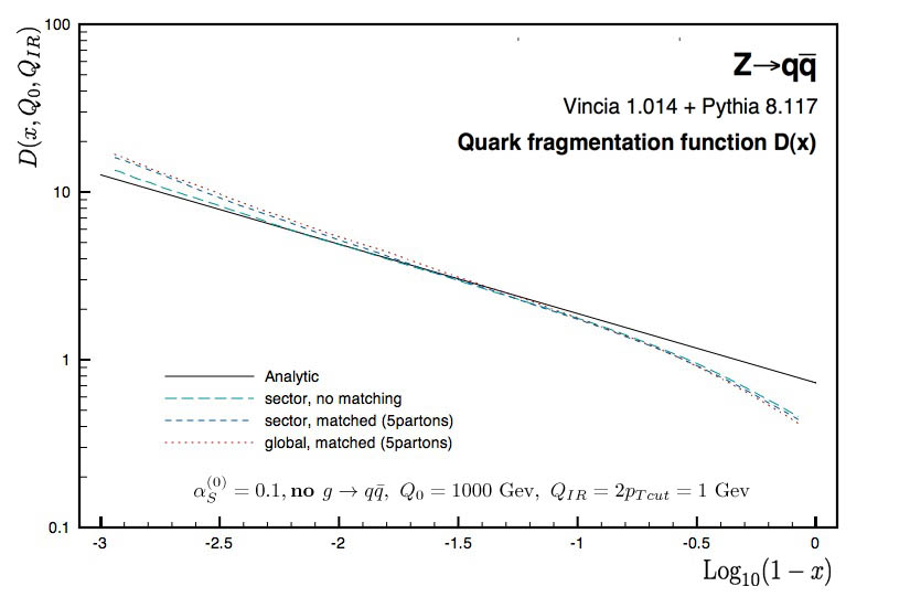
In addition to the LO matrix-element comparisons given in section 3.2, we have performed two basic tests of the all-orders sector shower implementation in Vincia interfaced to Pythia 8. First, we compare results obtained with just the perturbative Vincia shower (i.e., without switching on Pythia’s hadronization model) to a leading-logarithmic analytical resummation of the quark fragmentation function, similarly to what was done in [44]. We recall that the energy fraction is defined as
| (69) |
We use a constant value of , a starting scale of GeV, and an ending scale of GeV, for a perturbative evolution spanning three orders of magnitude in . This comparison is shown in Fig. 17, with and without matching, and also compared to the default (matched) global result, as a function of on the axis. The region on the right-hand side of the plot, , is dominated by hard emissions and is not expected to be well reproduced by the analytical soft resummation. Likewise, energy-momentum conservation effects are important, included in Vincia but neglected in the analytical resummation. It is therefore not surprising the analytical calculation differs from all of the Vincia ones in that region. On the left half of the plot, soft emissions dominate. One observes that the unmatched sector shower is quite close to the analytical result. The matching correction actually increases the difference slightly, which we interpret as due to our matching corrections being applied also in the soft region. The difference is consistent with similar variations observed by varying the LL finite terms in [44]. One also notes that the two matched calculations (global and sector) are consistent with each other.
As a second cross check, we include some comparisons to LEP event-shape data at , using light-flavor () data taken by the L3 collaboration [52]. In all cases, we include tree-level matching through partons, the default in Vincia. Between 1 and 2 million unweighted events were generated for each generator setting. These comparisons necessarily include the effects of hadronization. We have not attempted to do a full-fledged tuning of Pythia’s non-perturbative hadronization parameters for use with the sector shower. Instead, the default Vincia tune (summarized in Appendix B) is used, with the same value of the infrared cutoff (1 GeV) as in the global case.
With this setup, replacing the default global shower by the sector one with antenna functions as defined in this paper, we find that the sector shower produces slightly softer event shapes than the global one. A first illustration of this is given in the left-hand panes of figs. 18 and 19, in which we compare the sector and global shower implementations in Vincia to measurements of the Thrust and -parameter event-shape variables, which arise at and respectively (see [52] for a definition). For reference, the parameter, qualitatively similar to Thrust, is included in Appendix A, as are the Wide and Total Jet Broadening parameters. The result obtained with the sector shower is shown with thin (blue) lines, the global one with thick (red) lines. The upper pane of each plot shows the normalized event-shape distribution and the lower pane the ratio of the calculations to data.
In all the event shapes, the sector shower peaks at lower values than the corresponding global distribution. Since both showers include matching through partons, their tree-level expansions are equal up to the first three orders in . We therefore do not believe finite-term contributions alone could be responsible for the apparent “softness” of the sector shower relative to the global one. This conclusion is corroborated by the line labeled “ant=Max” in the right-hand pane of the figures (thick blue line), for which we replaced the sector antenna functions defined in this paper by the “Max” ones defined in [19], which have large finite terms; the result can be seen not to vary substantially from the sector curve shown in the left-hand panes, indicating that it is stable under finite-term variations.
Tentatively, our conclusion is that the difference between the distributions produced by the two shower models owes to a difference between the perturbative corrections generated beyond tree level, such as their choices and Sudakov form factors. To illustrate this, the thin (red) curves in the right-hand panes of figs. 18 and 19, labeled , show what happens if the value used to define the 1-loop running coupling in Vincia is changed from 0.139 to 0.143. (Note that these values should be interpreted in an LO scheme defined by Vincia, hence they are not immediately interpretable as, e.g., values.) This corresponds to a change in the 5-flavor value of from MeV to MeV and is sufficient to bring the sector shower into agreement with the result obtained with the global one. We note that this change may be connected with the question of whether it is still correct to use as the argument for in the sector shower, an issue we plan to return to in the context of a separate study [53].
At the non-perturbative level, the intrinsic softness of the sector shower also has consequences, as illustrated in the left-hand panes of fig. 20, where we compare to the distributions of the number (top row) and momentum fraction (bottom row) of charged particles, with . The sector shower defined in this paper (thin blue lines) produces a wider multiplicity distribution than the global one, with slightly more particles having . Again, the right-hand panes illustrate what happens when choosing larger finite terms (thick curve) and when choosing a larger value (thin lines). Similarly to above, the variation of antenna-function finite terms does not lead to substantial differences, while changing the value of does. It is evident that the sector shower, even with , could benefit from a slight retune of its non-perturbative parameters, e.g., to suppress the slightly overpopulated tails of low- and high-multiplicity events.
Further event-shape comparisons, and the production ratios of certain meson and baryon species, normalized to the average charged multiplicity, are given in Appendix A.
As emphasized in the preceding sections, one of the chief advantages of the sector shower approach is the fact that it only generates a single contributing term per phase-space point, for each order in perturbation theory. This makes it ideally suited for the GKS matching strategy [17], which requires at least one matrix-element-evaluation per contributing shower path. In tab. 4, we compare the number of milliseconds it takes to generate one event, between various programs and matching algorithms, using a standardized set-up. Since we are not interested in the speed of hadronization or hadron decay algorithms, we leave hadronization switched off and define an “event” as a perturbative cascade starting from a dipole at (with and using massive matrix elements for quarks), evolved down to the default perturbative cutoff scale in the respective code, which is of order 1 GeV in all cases.
In Pythia 6 [23] and 8 [43], only matching to the decay matrix element is available, hence speeds for higher multiplicity-matching are not shown in the table. We note that, at least in this test, Pythia 8 generates events as fast as Pythia 6.
The default (global, smoothly ordered) shower implementation in Vincia (third row) is slightly slower than the one in Pythia, which we regard as a consequence of the greater flexibility built into Vincia (smooth ordering, with generic evolution variables, antenna functions, and kinematics maps) combined with its more elaborate matching setup (taking explicit ratios of leading- and full-color MadGraph matrix elements [3] and evaluating them using Helas [47] routines). Using the GKS matching, however, Vincia’s matching may be extended to higher multiplicities, shown in the third to sixth columns. (All comparisons use matching to full-color matrix elements.) Since the number of matrix-element evaluations grows linearly with the multiplicity in the global approach, we see that the speed decreases quite rapidly with multiplicity.
In the sector approach, on the other hand (fourth row), the perturbative evolution is slightly slower at low matched multiplicities (basically since each gluon now requires two separate trial functions, and since no optimization of the trial phase-space has yet been implemented, relative to the global case), but the increase with multiplicity is less severe, resulting in the sector approach being faster than the global one starting from matching through .
In order to compare directly with other multileg approaches, such as the CKKW one [11] implemented in Sherpa [54], we have included the optional possibility to stop applying matching corrections below a specific value of the evolution scale in Vincia, thus emulating the “matching scale” that is present in the CKKW strategy. This obviously speeds up the calculation somewhat, since lots of soft emissions no longer need to have matching coefficients evaluated. For both Vincia and Sherpa, we set the matching scale equal to 5 GeV, ignoring that the phase-space contours defined by that value do not exactly match between the two codes. In the comparison to Sherpa, it is furthermore necessary to divide the total event-generation time up on a non-negligible initialization stage and a subsequent per-event time. In both Pythia and Vincia, the initialization time is essentially zero, while it grows with final-state complexity in Sherpa, due to the necessity of computing cross sections and initializing phase-space generators for each matrix-element configuration separately. The total event-generation time for Sherpa (bottom row in tab. 4) is therefore divided up on two numbers, with the initialization duration reported separately below the main per-event time. Even if one neglects the initialization component, however, it is clear that there is a significant speed difference between the two methods. Including the initialization time, the differences become even more pronounced. For example, during the 22 minutes it takes to initialize the CKKW generator for matching through partons (the default matching level in Vincia), the GKS implementation has time to generate almost 1 million matched showers. We stress that Sherpa is still obviously a much more versatile tool than Vincia, and hence this comparison is not intended as an advertisement for one code over another, rather its purpose is to test the dependence of the algorithmic speed on multiplicity, of the two matching prescriptions implemented in the respective generators. Note also that, while Vincia currently relies on MadGraph and Helas for its matrix elements, Sherpa uses the Comix generator [8]. We did not attempt to calibrate for this difference in this comparison, hence it is possible that the Vincia numbers, in particular for high matched multiplicities, could be reduced somewhat by implementing a faster matrix-element method.
Note also that the relative increase in per-event time for Sherpa actually becomes smaller with multiplicity. For instance, the per-event time only increases by a factor 2 when going from 5 to 6 partons, compared to factors of 4 and 10 at each of the preceding orders, respectively. We interpret this as being due to the fact that the corresponding cross sections, for exclusively66 6 For the highest matched multiplicity, replace exclusively by inclusively. resolved partons above the matching scale, are becoming increasingly small. Thus, once e.g. the 6-parton cross section has been computed (during initialization, the time for which still increases by an order of magnitude from 5 to 6 partons), the time to actually generate additional events does not increase substantially. This is very different from Vincia, in which the initialization time (zero) does not increase substantially, but the per-event time does.
6 Conclusions
We have presented a formalism for parton showers based on sector antennae, accompanied by an implementation in the Vincia plug-in [18] to the Pythia 8 event generator [43]. The main distinguishing feature of such showers is that only a single radiation antenna contributes to each phase-space point, as compared to a sum over all radiators in traditional “global” showers [34, 18, 36, 16]. The coefficients of the single poles of gluon antennae are modified to reflect this reorganization. A similar formalism including mass and polarization corrections has been developed in [40, 41], but has not yet been implemented in a publicly available event generator.
At the analytical level, we have tested the formalism by comparing tree-level expansions of it to fixed-order matrix elements for , , and partons. We find that the global shower, with its many terms, is able to deliver a somewhat better average agreement at the multileg level, in particular for processes involving splittings. To our minds, the advantage of the sector approach is therefore at present mainly a computational one, to be sought in the consequences of its simpler structure. Since the sector shower only produces a single term per phase-space point, it gives a speed advantage over the global approach when combined with the “GKS” matching formalism developed in [17], which requires at least one matrix-element-evaluation per contributing path. We demonstrate this speed gain by comparing global and sector showers matched to LO matrix elements through up to four branchings in Vincia. For reference, we also compare to an implementation of the CKKW method for multileg matching [11], using the Sherpa generator [54].
As a final cross-check, we have also compared the sector shower implementation in Vincia, with and without matching, to an analytic resummation of the quark fragmentation function and to experimental measurements of event shapes and related quantities at LEP. We find that the present sector shower implementation appears to be consistent with these distributions, within the expected precision, and hence consider it validated and ready to be used for other phenomenology studies.
Nevertheless, since the sector shower a priori produces slightly more particles with and somewhat softer event-shape distributions, we recommend to increase the value of from 0.139 in the default tune to for use with the sector shower. This results in good agreement with event shapes but still generates a slightly too broad charged-particle multiplicity distribution. Depending on the application, a further iteration of the non-perturbative tuning, focusing specifically on sector showers, could therefore also be interesting to explore.
Acknowledgments
We thank A. Gehrmann-de-Ridder, W. Giele, D. Kosower, A. Larkoski, M. Peskin, M. Ritzmann, and J. Winter, for many enjoyable discussions on the singularity structure of antenna showers. We thank D. Kosower in particular for pointing out the subtlety connected with the choice of sector decomposition variable for gluon splittings and for suggesting the modification necessary to cure it.
This work was supported in part by the Marie Curie FP6 research training network “MCnet” (contract number MRTN-CT-2006-035606), as well as by the European Commission (HPRN-CT- 200-00148), FPA2009-09017 (DGI del MCyT, Spain) and S2009ESP-1473 (CA Madrid). J.J. L-V is supported by a MEC grant, AP2007-00385, and wants to thank the CERN Theory Division for its hospitality.
Appendix A Additional LEP Comparisons
This appendix contains some further comparisons of the sector shower with LEP distributions, as follows: the event-shape variable (fig. 21), and the Wide and Total Jet broadening parameters (figs. 22 and 23, respectively), defined as in [52], to which we compare. We also compare the production rates of selected identified baryon and meson species, normalized to the average charged-particle multiplicity, to our own average over the various identified-particle measurements performed at LEP [55, 56] (fig. 24).
Appendix B Tune Parameters
The default tune of Vincia 1.0.27 is “Jeppsson4”, an update of the original “Jeppsson” tune presented in [17]. The parameters are optimized for use with the global shower (the default in Vincia) but are here used for the sector shower as well, with comments as given in section 5. The Jeppsson4 tune is characterized by the following parameters:
! * VINCIA alphaS
Vincia:alphaSValue        = 0.139
Vincia:alphaSscaleFactor  = 0.5
Vincia:alphaSorder        = 1
Vincia:alphaSmode         = 3
! * VINCIA Shower cutoff scale
Vincia:cutoffType         = 1
Vincia:cutoffScale        = 1.0
! * PYTHIA String fragmentation parameters
StringZ:aLund             = 0.55
StringZ:bLund             = 0.95
StringZ:aExtraDiquark     = 1.0
StringPT:sigma            = 0.275
StringPT:enhancedFraction = 0.01
StringPT:enhancedWidth    = 2.0
! * PYTHIA String breakup flavor parameters
StringFlav:probStoUD     = 0.20
StringFlav:mesonUDvector = 0.45
StringFlav:mesonSvector  = 0.7
StringFlav:probQQtoQ     = 0.085
StringFlav:probSQtoQQ    = 1.00
StringFlav:probQQ1toQQ0  = 0.035
StringFlav:decupletSup   = 1.0
StringFlav:etaSup        = 0.68
StringFlav:etaPrimeSup   = 0.085
References
- [1] A. Pukhov, 2004, hep-ph/0412191.
- [2] E. Boos et al., Nucl.Instrum.Meth. A534 (2004) 250, [hep-ph/0403113].
- [3] J. Alwall et al., JHEP 0709 (2007) 028, [0706.2334].
- [4] A. Kanaki, C. G. Papadopoulos, Comput.Phys.Commun. 132 (2000) 306, [hep-ph/0002082].
- [5] F. Krauss, R. Kuhn, G. Soff, JHEP 0202 (2002) 044, [hep-ph/0109036].
- [6] M. Moretti, T. Ohl, J. Reuter, 2001, hep-ph/0102195.
- [7] M. Bähr et al., Eur.Phys.J. C58 (2008) 639, [0803.0883].
- [8] T. Gleisberg, S. Hoeche, JHEP 0812 (2008) 039, [0808.3674].
- [9] P. Skands, 2011, 1104.2863.
- [10] J. Alwall et al., Eur. Phys. J. C53 (2008) 473, [0706.2569].
- [11] S. Catani, F. Krauss, R. Kuhn, B. R. Webber, JHEP 11 (2001) 063, [hep-ph/0109231].
- [12] F. Krauss, JHEP 08 (2002) 015, [hep-ph/0205283].
- [13] L. Lonnblad, JHEP 05 (2002) 046, [hep-ph/0112284].
- [14] S. Mrenna, P. Richardson, JHEP 05 (2004) 040, [hep-ph/0312274].
- [15] N. Lavesson, L. Lönnblad, JHEP 04 (2008) 085, [0712.2966].
- [16] A. Buckley et al., Phys.Rept. 504 (2011) 145, [1101.2599].
- [17] W. Giele, D. Kosower, P. Skands, 2011, 1102.2126.
- [18] W. T. Giele, D. A. Kosower, P. Z. Skands, Phys.Rev. D78 (2008) 014026, [0707.3652].
- [19] A. G.-D. Ridder, M. Ritzmann, P. Skands, 2011, 1108.6172.
- [20] P. D. Draggiotis, A. van Hameren, R. Kleiss, Phys.Lett. B483 (2000) 124, [hep-ph/0004047].
- [21] C. W. Bauer, F. J. Tackmann, J. Thaler, JHEP 0812 (2008) 011, [0801.4028].
- [22] M. Bengtsson, T. Sjostrand, Phys.Lett. B185 (1987) 435.
- [23] T. Sjöstrand, S. Mrenna, P. Z. Skands, JHEP 05 (2006) 026, [hep-ph/0603175].
- [24] P. Nason, G. Ridolfi, JHEP 0608 (2006) 077, [hep-ph/0606275].
- [25] S. Frixione, P. Nason, C. Oleari, JHEP 0711 (2007) 070, * Temporary entry *, [0709.2092].
- [26] G. Altarelli, G. Parisi, Nucl. Phys. B126 (1977) 298.
- [27] G. Marchesini, B. R. Webber, Nucl. Phys. B238 (1984) 1.
- [28] M. Bengtsson, T. Sjostrand, Nucl.Phys. B289 (1987) 810.
- [29] T. Sjöstrand, P. Z. Skands, Eur. Phys. J. C39 (2005) 129, [hep-ph/0408302].
- [30] S. Catani, M. H. Seymour, Nucl. Phys. B485 (1997) 291, [hep-ph/9605323].
- [31] Z. Nagy, D. E. Soper, JHEP 09 (2007) 114, [0706.0017].
- [32] M. Dinsdale, M. Ternick, S. Weinzierl, Phys. Rev. D76 (2007) 094003, [0709.1026].
- [33] S. Schumann, F. Krauss, JHEP 03 (2008) 038, [0709.1027].
- [34] G. Gustafson, U. Pettersson, Nucl. Phys. B306 (1988) 746.
- [35] L. Lönnblad, Comput. Phys. Commun. 71 (1992) 15.
- [36] J.-C. Winter, F. Krauss, JHEP 07 (2008) 040, [0712.3913].
- [37] D. A. Kosower, Phys.Rev. D57 (1998) 5410, [hep-ph/9710213].
- [38] D. A. Kosower, Phys. Rev. D71 (2005) 045016, [hep-ph/0311272].
- [39] A. Gehrmann-De Ridder, T. Gehrmann, E. Glover, JHEP 0509 (2005) 056, Erratum added online, 8/18/06, [hep-ph/0505111].
- [40] A. J. Larkoski, M. E. Peskin, Phys.Rev. D81 (2010) 054010, [0908.2450].
- [41] A. J. Larkoski, M. E. Peskin, Physical Review D (2011), [1106.2182].
- [42] http://projects.hepforge.org/vincia/.
- [43] T. Sjöstrand, S. Mrenna, P. Z. Skands, Comput. Phys. Commun. 178 (2008) 852, [0710.3820 [hep-ph]].
- [44] P. Z. Skands, S. Weinzierl, Phys.Rev. D79 (2009) 074021, [0903.2150].
- [45] A. Gehrmann-de Ridder, M. Ritzmann, P. Skands, 2011, CERN-PH-TH/2011-113.
- [46] R. Kleiss, W. Stirling, S. Ellis, Comput.Phys.Commun. 40 (1986) 359.
- [47] H. Murayama, I. Watanabe, K. Hagiwara, 1992.
- [48] J. Lopez-Villarejo, P. Skands, 2011, work in progress (Les Houches, 2011).
- [49] A. Gehrmann-De Ridder, T. Gehrmann, E. Glover, Nucl.Phys. B691 (2004) 195, [hep-ph/0403057].
- [50] A. Gehrmann-De Ridder, T. Gehrmann, E. Glover, Phys.Lett. B612 (2005) 36, [hep-ph/0501291].
- [51] A. Gehrmann-De Ridder, T. Gehrmann, E. Glover, Phys.Lett. B612 (2005) 49, [hep-ph/0502110].
- [52] L3 Collaboration Collaboration, P. Achard et al., Phys.Rept. 399 (2004) 71, [hep-ex/0406049].
- [53] L. Hartgring, E. Laenen, P. Skands, 2011, in preparation.
- [54] T. Gleisberg et al., JHEP 0902 (2009) 007, [0811.4622].
- [55] G. Lafferty, P. Reeves, M. Whalley, J.Phys.G G21 (1995) A1.
- [56] Particle Data Group Collaboration, K. Nakamura, J. Phys. G37 (2010) 075021.