IPPP/11/48
DCPT/11/96
Edinburgh 2011/22
DFTT-24/2011
The infrared structure of gauge theory amplitudes in the high-energy limit
Abstract
We develop an approach to the high-energy limit of gauge theories based on the universal properties of their infrared singularities. Our main tool is the dipole formula, a compact ansatz for the all-order infrared singularity structure of scattering amplitudes of massless partons. By taking the high-energy limit, we show that the dipole formula implies Reggeization of infrared-singular contributions to the amplitude, at leading logarithmic accuracy, for the exchange of arbitrary color representations in the cross channel. We observe that the real part of the amplitude Reggeizes also at next-to-leading logarithmic order, and we compute the singular part of the two-loop Regge trajectory, which is universally expressed in terms of the cusp anomalous dimension. Our approach provides tools to study the high-energy limit beyond the boundaries of Regge factorization: thus we show that Reggeization generically breaks down at next-to-next-to-leading logarithmic accuracy, and provide a general expression for the leading Reggeization-breaking operator. Our approach applies to multiparticle amplitudes in multi-Regge kinematics, and it also implies new constraints on possible corrections to the dipole formula, based on the Regge limit.
Keywords
perturbative QCD, resummation, Regge limit, soft singularities1 Introduction
It is well known that the structure of gauge theory scattering amplitudes simplifies dramatically in the high-energy limit, in which the centre-of-mass energy is much larger than the typical momentum transfer , or, alternatively, , with held fixed. Studies of this limit predate QCD, and formed the basis of Gribov-Regge theory (see for example [1, 2, 3] and references therein), in which the analytic properties of amplitudes were considered in the complex angular momentum plane, independently of any underlying field theory; the high-energy limit is thus often referred to as the Regge limit. The asymptotic form of scattering amplitudes in this limit is determined by the structure of singularities in the complex angular momentum plane. If simple poles are present, for example, the amplitude takes the form
| (1) |
for some prefactor function , where is the Regge trajectory associated with the right-most pole in the complex angular momentum plane, which can be physically interpreted in terms of the exchange of a family of particles in the -channel. Multiple poles or cuts give rise to a more complicated -dependence, in addition to the power-like growth described by eq. (1).
The high-energy limit has also been extensively studied within the context of perturbative quantum field theory. In a variety of theories, amplitudes may display the phenomenon of Reggeization: specifically, amplitudes for scattering are dominated, in the Regge limit, by -channel exchanges of particles whose propagators become dressed according to the schematic form11 1 For spin 1 gauge bosons, eq. (2) may be taken to represent the Feynman gauge result.
| (2) |
This perturbative result leads to amplitudes which are consistent with Regge theory expectations, i.e. having the form of eq. (1), with the two functions and related by an integer additive constant. The function is thus usually referred to as the Regge trajectory of the corresponding particle.
The history of Reggeization studies in quantum field theory is by now a lengthy one, beginning with the work of [4, 5, 6, 7, 8, 9]. In QED, at leading logarithmic (LL) accuracy, the electron is found to Reggeize [4, 10], but the photon does not [5, 11, 12, 13]. In QCD it has been shown that both the gluon [14] and the quark [15] Reggeize at LL accuracy. Those proofs are based on the gluon [16, 17, 18, 19, 20, 21, 22] and quark [23, 24, 25] Regge trajectories to one-loop order, which are necessary to generate all leading logarithms of in the scattering amplitude22 2 For a pedagogical review of Reggeization at one loop in QCD, see [26, 27].. The two-loop gluon [28, 29, 30, 31, 32] and quark [33] Regge trajectories have also been computed. Reggeization, however, has been proven to next-to-leading logarithmic order (NLL) only for the gluon [34]. Furthermore, contributions beyond NLL order have been considered in the simpler context of an Super-Yang-Mills (SYM) theory (see section 5 in [35] as well as Refs. [36, 37]). The proof of Reggeization to a given logarithmic accuracy, but to all orders in perturbation theory (corresponding to a fixed loop order in the Regge trajectory) typically involves a careful iterative argument, which shows that kinematic information at any given fixed order is consistent with the form of eq. (2), and also that the color factor at each order is proportional to that of the appropriate single-particle exchange graph.
An alternative approach [38, 39, 40, 41, 42, 43] uses the fact that scattering in the Regge limit can be described by a pair of Wilson lines33 3 A general discussion of the role of Wilson lines in the high-energy limit of QCD was given in [44]., and exploits the renormalisation properties of the latter to derive the gluon Regge trajectory up to two loops, as well as an all-order expression [41] for the singular part of the trajectory in terms of an integral over the cusp anomalous dimension [45, 46, 47, 48, 49]. We shall reproduce these results in the present paper using a different theoretical framework.
Aside from being of conceptual interest in making contact between the high-energy limit of perturbative quantum field theories and the known constraints of Gribov-Regge theory, Reggeization is a highly important result both in view of phenomenological applications and as a tool for the theoretical analysis of gauge theory amplitudes. For example, it is a crucial ingredient in the BFKL equation [22, 20, 21, 50], an integral equation for the gluon four-point function in the Regge limit, whose singlet solution describes the -channel exchange of a Reggeized object having the quantum numbers of the vacuum (the Pomeron). Phenomenological applications of the BFKL equation (and related results concerning the factorized structure of scattering amplitudes in the Regge limit) are wide-ranging and constitute a field of research too vast to be summarized here. On the theoretical side, the high-energy limit has been instrumental in several recent studies concerning the all-order structure of gauge theory amplitudes: for example, corrections to the BDS conjecture [51] for the iterative structure of scattering amplitudes in planar SYM were analyzed in [36, 52, 53, 54], and properties of the Regge limit were used in [55, 56, 57] for the calculation of light-like polygonal Wilson loops, which are conjectured to be dual to maximally helicity violating scattering amplitudes in this particular theory [58, 35, 59].
In this paper we consider the high-energy limit of gauge theory amplitudes from a novel viewpoint, and we relate Regge factorization to the universal structure of infrared singularities of massless gauge theories [60]. Our approach is motivated by the well-known observation that the Regge trajectory is infrared divergent in perturbation theory, since it arises formally as an integral over the loop transverse momentum, which always diverges in the presence of massless gauge bosons. As a consequence, it must be possible to employ our understanding of the universal properties of infrared radiation in order to study the high-energy limit in general, and Reggeization in particular. Clearly, finite contributions to the Regge trajectory, which are known to arise starting at NLL, will be outside the domain of applicability of our method. As we will see, however, our approach will allow us to draw very broad conclusions concerning both the generality and the limitations of the phenomenon of Reggeization, and will provide us with tools to analyze the high-energy limit beyond the limits of Regge factorization.
The factorization and exponentiation of soft and collinear singularities have been actively studied for several decades (see, for example [61, 62, 63, 64, 65, 66, 67, 68]); only recently, however, has a general all-order understanding of the anomalous dimensions that govern infrared exponentiation for multiparticle amplitudes in non-abelian gauge theories begun to emerge. For massless gauge theories, current knowledge is summarized in the dipole formula [69, 70, 71, 72], a recently proposed ansatz for the all-order infrared singularity structure of general fixed-angle scattering amplitudes of massless partons, which we will review in more detail in Sec. 1.2. Briefly, the essential idea of infrared exponentiation is that all IR singularities, which appear as poles in dimensional regularisation (in dimensions, with ) may be encapsulated in an exponential operator acting on a hard interaction which is finite as . The exponent contains in principle terms which couple kinematic and color dependence of all hard partons. The dipole formula, however, posits that for massless amplitudes correlations exist only between pairs of hard particles (i.e. there are no irreducible correlations between three or more partons, a fact which is not true for massive particles [73, 74, 75, 76, 77, 78, 79, 80, 81]). Furthermore, the coefficients of these dipole correlations are governed purely by the cusp anomalous dimension [45, 46, 47, 48, 49] and by the beta function. The dipole formula is known to be exact up to two loop order in the exponent, for any number of massless hard partons. Possible corrections at higher orders are strongly constrained [70, 71, 82], as we discuss below in Sec. 1.2.
By applying the dipole formula in the case of scattering in the high-energy limit, we will show explicitly that, at leading-logarithmic accuracy44 4 By LL accuracy we mean the ability to predict the coefficients of the largest powers of arising to all orders, regardless of possible overall powers of which might be present for a given observable. Thus if the first logarithm of arises at order , leading logarithms are of the form ., Reggeization of allowed -channel exchanges is a completely general phenomenon, which takes place for arbitrary color representations exchanged in the crossed ( or ) channel. The relevant one-loop Regge trajectory in each case involves the quadratic Casimir invariant of the appropriate representation of the gauge group, generalising what is already known about the quark and gluon Regge trajectories. Next, given the all-order nature of the dipole formula, we will also be able to examine Reggeization beyond leading logarithmic accuracy. We will show that, for the singular terms of the Regge trajectory, Reggeization holds also at NLL accuracy and with the same degree of generality, but only for the real part of the amplitude. We will also show that the singular terms of the Regge trajectory are given by a simple integral of the cusp anomalous dimension over the scale of the running coupling, as already derived in [38, 39, 40, 41] using Wilson lines. Beyond NLL order, however, we will provide evidence for the breakdown of Reggeization through the appearance in the perturbative exponent of color operators that survive in the high-energy limit but in general cannot be diagonalized simultaneously with the ones responsible for (or ) channel exchange. We further show that Reggeization breaking will take place at NNLL independently of the precise form of the three-loop soft anomalous dimension; conversely, we also use the Regge limit to derive new constraints on potential three-loop corrections to the soft anomalous dimension going beyond the dipole formula, extending the results of Ref. [82]. Finally, we generalize our discussion to the case of scattering, in multi-Regge kinematics. Also in this general case, we show that the dipole formula implies LL Reggeization in the crossed channel, according to the standard ansatz employed in the multi-Regge limit [26], and we observe the same pattern of partial generalization to higher logarithmic accuracy that arises for the four-point amplitude. In general, our approach, while focused on divergent contributions to the high-energy limit, goes beyond the limitations of Regge factorization, and gives results that are valid to arbitrary logarithmic accuracy and for general color exchanges.
The structure of the paper is as follows. In the remainder of this introduction, we will review relevant information regarding both the high-energy limit of amplitudes and the dipole formula. In Sec. 2 we will present our argument for Reggeization based on the dipole formula, by considering the Regge limit of the four-point amplitude and examining the action of the infrared-singular operator on hard interactions involving a definite -channel exchange. Using this formalism we will reproduce in Sec. 3 the known form of gluon-gluon scattering at leading logarithmic order, and show that this result generalises to exchanges involving particles in different representations of the gauge group. In Sec. 4 we consider the Regge trajectory at higher order in the perturbative expansion, and construct explicitly the color operator responsible for the expected breakdown of Reggeization at NNLL. In Sec. 5 we use the reverse logic and demonstrate that the Regge limit provides a useful constraint on potential corrections to the dipole formula at three loops and beyond. In Sec. 6 we generalize our basic argument to the case of -particle amplitudes in multi-Regge kinematics. Finally, we discuss our results in Sec. 7 before concluding.
1.1 The high-energy limit: an outline
In this section, we give a slightly more detailed presentation of known results on the high-energy limit of scattering amplitudes, introducing concepts and notations that will be useful in the following sections. We will focus in particular on gluon and quark scattering, preparing for the more general discussion of Sec. 3.
Let us consider first the case of scattering, whose leading-order Feynman diagrams are shown in fig. 1.
While the high-energy limit of the amplitude is, of course, gauge invariant, it is useful to refer to a diagrammatic picture in which the dominant contribution at large (up to power-suppressed terms) is obtained from a single diagram. Indeed, in an appropriate gauge (see e.g. Sec. 2.4 in Ref. [26]), of the four possible diagrams – involving , and -channel exchanges, and a four-gluon vertex, respectively – only the -channel exchange diagram of fig. 1(b) contributes in the Regge limit55 5 Note that keeping only diagram (b) violates gauge invariance, but only by terms which are suppressed in the Regge limit., with the others suppressed by powers of . The leading order (LO) contribution in the Regge limit thus has a single color structure, namely that associated with a -channel color-octet exchange.
Higher-order contributions in scattering might in general involve additional color structures, besides the pure octet exchange observed at tree level, even in the Regge limit. There are two reasons for this: first, beyond LO there could be contributions not described by pure -channel exchange; second, even if pure -channel exchange dominates, there may be different possible color structures at higher orders. Indeed, one can enumerate the possible color quantum numbers exchanged in the channel by taking the product of the color representations of the particles labeled 1 and 3 in fig. 1(b), which in the present case are gluons, belonging to the adjoint representation of , and decomposing it into irreducible representations as
| (3) |
where we introduced indices to distinguish the (antisymmetric) adjoint representation from the 8-dimensional symmetric representation. One sees explicitly that a color-octet exchange is only one of a number of possibilities, and predicting which ones will contribute in the Regge limit requires further theoretical input. This input is provided by the observation that, at least for leading logarithms, the diagrams that contribute to the Regge limit correspond to the exchange of a gluon ladder in the channel [12, 17, 22]. As we will see shortly, this also constrains the color structure of the amplitude. The non-trivial nature of the Reggeization property is thus twofold, involving both color and kinematics: the leading kinematic behaviour at each order in the coupling constant involves logarithms of precisely so as to produce the power-like dependence given by eq. (2); also, the color factor at each order in perturbation theory is proportional to that of the tree level exchange. In other words, of the possible -channel exchanges listed in eq. (3), only the octet exchange survives at leading logarithmic order in the Regge limit, with other possible color factors being kinematically suppressed, either by logarithms or powers of .
Calculating the amplitude for exchange of a Reggeized gluon, to LL accuracy, gives a matrix element of the form [17, 22]
| (4) |
where and are the color index and momentum of gluon (with labelling as in figure (1b)), and is a color generator in the adjoint representation, so that . The coefficient functions , usually referred to as impact factors, depend on the helicities [83, 84] of the gluons (or on the spin polarizations [22] in the case of quarks), and may contain collinear singularities associated with them, but, as the notation suggests, carry no dependence. In the high-energy limit helicity is conserved across the vertices, so only certain impact factors are relevant (see [84] for more details). Equation (4) is an example of Regge factorization: the impact factors are universal (process-independent), reflecting the properties of the scattered partons, while the states exchanged in the channel appear only through their Reggeized propagator.
A further important ingredient in the computation of the Regge limit is the observation that the matrix element must have even parity under exchange, which follows from the assumption that only -channel gluon ladders contribute. It is easy to see that, at leading logarithmic accuracy, the kinematic part of eq. (4) is odd under exchange, due to the overall factor of . Indeed, Mandelstam invariants satisfy, for massless particles, the momentum conservation relation
| (5) |
which in the Regge limit implies
| (6) |
leading to an overall sign change when is replaced by . This, in turn, requires that the color structure of the amplitude should also be odd under the same exchange. Once again, this is true for Reggeized gluon exchange, since
| (7) |
if we take the generators in the (antisymmetric) color octet representation. The color factor on the right-hand side is that of the process , whose amplitude (by crossing symmetry) is equal to that of eq. (4) upon replacing with . One may then rewrite eq. (4) to display explicitly the symmetry under exchange, as
| (8) |
One observes that the symmetry requirement under exchange, together with the negative parity (usually called ‘signature’ in this context) of the kinematic part of the amplitude, force the color representation exchanged in the channel to be antisymmetric. Notice however that this requirement does not uniquely select the (antisymmetric) octet in eq. (3): either of the two decuplet representations would also be allowed. That only the octet actually contributes to the reggeized amplitude at LL (and indeed at NLL as well) is a result of the detailed proof of Reggeization [14, 34].
Similar expressions are obtained for quark-quark or quark-gluon scattering, where the only modification in eq. (4) is that the color generators and the coefficient functions are replaced by those belonging to the appropriate representation. Crucially, however, the Regge trajectory is a universal object: it is a property of the particle exchanged in the channel, and does not depend on the identities of the external particles. More precisely, the gluon Regge trajectory , appearing in eq. (4) and in eq. (8) can be expressed as
| (9) |
where we expanded the trajectory in terms of the -dimensional running coupling
| (10) |
with , and for infrared regularization. According to eq. (8), truncating eq. (9) to first order, one finds that only the octet of negative signature gives contributions of the form in the -loop amplitude. This is the statement of the Reggeization of the gluon to LL accuracy [14]. The result for the one-loop gluon trajectory is
| (11) |
where is the quadratic Casimir invariant for the adjoint representation, as is appropriate for the exchange of a gluon, and we have introduced the one loop coefficient of the universal cusp anomalous dimension [45, 46, 47, 48, 49] (to be discussed in more detail in Sec. 1.2), , following the notation of Ref. [70]. Together with the effective vertex for the emission of a gluon along the ladder [17], Reggeization of the gluon is a key prerequisite for the derivation of the BFKL equation at LL accuracy [21, 50].
In order to generalize the idea of Reggeization to multiparticle emission, one may begin by considering the amplitude for scattering. Each emitted gluon may be characterized by its rapidity in the center-of-mass frame of the collision, given by , with the longitudinal momentum of the -th gluon. High-energy logarithms arise then in the limit of strongly ordered rapidities of the outgoing gluons, with the transverse momenta of comparable size,
| (12) |
where, without loss of generality, we have taken the rapidities as decreasing. Note that we have labelled momenta and color indices as in fig. 2.
With these conventions, the amplitude for scattering can be written as [17]
| (13) | |||||
with , , and for . The effective vertex for the emission of a positive helicity gluon along the ladder, also known as the Lipatov vertex [17, 85, 83], is given by
| (14) |
where we use the complex momentum notation . The corresponding vertex for a negative helicity gluon, , is obtained by taking the complex conjugate of eq. (14). One may generalize eq. (12) to scattering, which is usually referred to as multi-Regge kinematics. The emission of a single gluon along the ladder iterates in an obvious fashion, so as to describe the emission of any number gluons (see [26] for a pedagogical review), and eq. (13) generalizes accordingly [22]. The amplitude for scattering, with emission of many gluons along the ladder, is related via unitarity to the BFKL equation [21, 50], and it will be discussed in Sec. 6 in the context of the dipole formula.
Reggeization of the gluon has also been proven to next-to-leading logarithmic (NLL) accuracy in QCD [34], implying that only the octet contributes to the term of the -loop amplitude, with the two-loop gluon Regge trajectory [28, 29, 30, 31, 32], given by66 6 Note that the sign of the double pole term in eq. (15) is the opposite of the one found, for example, in [32]: this is due to the fact that here we are expanding the Regge trajectory in terms of the renormalized coupling, rather than the bare coupling, as was done in [32].
| (15) |
where we introduced the one-loop -function coefficient , and the two-loop cusp anomalous dimension , given by [45, 46, 47, 48, 49]
| (16) |
Together with the coefficient functions for the emission of two gluons or two quarks along the ladder [86, 87, 88, 89], and the one-loop corrections to the emission of one gluon along the ladder [90, 91, 92, 93, 94], the two-loop gluon Regge trajectory constitutes a building block of the BFKL equation at NLL accuracy [95, 96, 97].
With similar methods, one may also examine Reggeization of the quark, using the scattering process , as shown in fig. 3.
In the limit this process is dominated by gluon exchange in the -channel (not displayed in fig. 3), as was the case for gluon-gluon scattering. One may however consider the alternative high-energy limit , . Note that in the center-of-mass frame of two-particle scattering one has , so the limit corresponds to backward scattering, in contrast to the forward scattering associated with -channel exchange in the Regge limit . This alternative high-energy limit is dominated by quark exchange: again, there are three diagrams at tree level, displayed in fig. 3, and only the diagram of figure 3(c), representing scattering via -channel quark exchange, contributes at leading power in . As in the case of -channel exchange, Reggeization amounts to the statement that the propagator for the exchanged quark becomes dressed, through virtual corrections, by a factor
| (17) |
where is the quark Regge trajectory. In particular, as was the case for gluon exchange, the color structure of the tree level interaction is preserved to all orders in the perturbation expansion, at least at LL level. The relevant color factor in this case has positive parity under the interchange of particles 2 and 3 (with labels as in figure (3c)), corresponding to the interchange . The amplitude may thus be written in a form which has manifestly positive signature in the -channel.
By analogy to what was done in eq. (9), one may expand the quark trajectory as
| (18) |
where the running coupling, defined as in eq. (10), is now evaluated with reference scale . The result for the one-loop quark Regge trajectory is [25]
| (19) |
with the quadratic Casimir invariant of the fundamental representation, appropriate to the exchange of a quark77 7 Note that a similar result holds in QED, where the electron also Reggeizes [4, 98, 99, 10].. Truncating eq. (18) to first order is equivalent to claiming that only the triplet of positive signature contributes to the term of the -loop amplitude, i.e. states the Reggeization of the quark to leading logarithmic accuracy [15]. The two-loop quark Regge trajectory was computed in [33], and reads
| (20) |
Note that eq. (20) has the remarkable feature that if one replaces everywhere with one obtains the two-loop gluon Regge trajectory in eq. (15). Specifically, the pole terms in are the same as in the two-loop gluon Regge trajectory, up to the interchange of the overall factor , a fact that will be precisely understood in our approach. Finite terms contain a contribution proportional to the difference : this would vanish for fermions in the adjoint representation, characteristic of supersymmetric gauge theories. Note that Reggeization of the quark to NLL accuracy has never been proven: in fact, for both the gluon and the quark trajectories, the calculation of the -loop Regge trajectory, which requires a -loop fixed-order calculation, has so far always predated the proof of the corresponding Reggeization to accuracy, which requires an all-order analysis.
In this section we have reviewed various details regarding Reggeization, which are relevant for the remainder of this paper. In particular, we have seen that both the quark and the gluon Reggeize in QCD, at least at LL level. Furthermore, the singular parts of their Regge trajectories are completely determined, at least at two loops, by the cusp anomalous dimension and by the beta function, and they only differ by the replacement of the overall quadratic Casimir invariant corresponding to the exchanged particle (in the and channels for quark and gluon exchanges, respectively).
1.2 The dipole formula
In this section, we review the dipole formula of [70, 69, 71], which will be used in Sec. 2 to investigate Reggeization. The formula is a closed form result for the anomalous dimension matrix which generates all infrared (soft and collinear) singularities of arbitrary fixed-angle scattering processes involving only massless external partons, and was first derived in [70, 69, 71]88 8 For a pedagogical review, see also [72]. The proportionality of the all-order anomalous dimension matrix to the one-loop result was conjectured in [100], after the two-loop calculation of [101].. Here we briefly summarise the derivation of [70], in order to make clear the origin (and possible limitations) of the dipole formula, as well as to introduce notation which will be useful in what follows.
Our starting point is a generic fixed-angle scattering amplitude for massless partons, shown schematically in fig. 4(a).
Parton momenta satisfy , and the invariants are all taken to be large relative to , and are assumed to be parametrically of the same size. Each parton carries a color index , and one may write the scattering amplitude as a vector in the space of possible color flows,
| (21) |
where is a suitable basis of color tensors for the process at hand. The amplitude contains long distance singularities, which may be traced to soft and collinear regions of integration in loop momentum space (see e.g. [102]). Many years of studies [62, 63, 64, 65, 68, 103, 104, 101, 105], have established that soft and collinear radiation has universal properties which lead to the fact that the associated singularities can be factorized from the complete amplitudes. Specifically, one may write the subamplitudes in eq. (21) in the factorized form99 9 A similar form has recently been explored in the context of perturbative quantum gravity [106, 107, 108].
| (22) | |||||
where is the 4-velocity of parton , and an auxiliary vector associated with each hard parton1010 10 The factors of two in the arguments of the various functions in eq. (22) are conventional and do not play a significant role in the present discussion., and such that . Here is the hard function, which is free of infrared singularities and thus finite as after renormalization. The soft function collects all soft singularities (including those which are both soft and collinear), and acts as a matrix in color flow space, owing to that fact that soft gluon emissions transfer color between the external hard parton lines. The soft function may be written as a vacuum expectation value of a renormalized product of Wilson-line operators acting on the color flow basis . One finds
| (23) |
where each Wilson-line operator may be written, as usual, as a path ordered exponential
| (24) |
The jet functions in eq. (22) collect collinear singularities associated with parton line , including those that are both collinear and soft. In terms of the auxiliary vector , and taking as an example the case of an external quark, one has
| (25) |
It is important to note that the jet functions are diagonal in color flow space, and they depend only on the quantum numbers of the single parton . Note further that singularities which are both soft and collinear appear in both the soft function and in the jet functions . One corrects for this double counting, as shown in eq. (22), by dividing by the eikonal jet functions , which are simply defined as the eikonal approximations to the partonic jet functions . They can thus be expressed in terms of Wilson lines as
| (26) |
The soft function of eq. (23) satisfies the evolution equation
| (27) |
a consequence of the fact that Wilson lines renormalize multiplicatively [109, 110, 111, 112]. The anomalous dimension , however, is singular as , due to the fact that the soft function still contains collinear singularities. Related to this is the fact that the functional dependence of the soft function involves the scalar products , which are not invariant under rescalings of the 4-velocities , as one would expect from the formal definition of the soft function in terms of semi-infinite Wilson lines. As analysed in detail in [70], these facts are both consequences of the cusp singularity of massless Wilson lines [45, 46, 47, 48, 49], whose properties are dictated by the cusp anomalous dimension to all orders in perturbation theory.
One may restore rescaling invariance by considering the reduced soft function [105, 70]
| (28) |
This function is free of collinear poles, which are removed by dividing out the eikonal jets. It must then follow that the anomaly in rescaling invariance, which was due to collinear singularities, has also been cancelled. The reduced soft function must then depend on the velocities in a rescaling-invariant manner, and this requirement leads to the fact that the kinematic dependence on the left-hand side of eq. (28) is through the quantities
| (29) |
which are indeed manifestly invariant under the transformation . The phases are defined by , where if and are both initial-state partons, or both final-state partons, and otherwise.
The reduced soft function in eq. (28) satisfies an evolution equation identical in form to eq. (27),
| (30) |
In this case however the anomalous dimension matrix is finite as , since the reduced soft function is free of collinear singularities. The restoration of the symmetry under rescaling transformations can be further exploited, using (28) and the properties of the jet functions , to derive a set of equations [70] that tightly constrain the functional dependence of the anomalous dimension matrix . They take the form
| (31) |
This is a set of independent differential equations for the matrix-valued soft anomalous dimension, which explicitly couple color and kinematic degrees of freedom. In order to write down the minimal solution to eq. (31), which leads to the announced dipole formula, it is useful to switch to a slightly more formal, basis-independent notation for color exchange. This is achieved by introducing color-insertion operators , following the notation of Catani and Seymour [113, 114]. The color operator acts as the identity on the color indices of all external partons other than parton , and it inserts a color generator in the appropriate representation on the -th leg. Using this compact notation, color conservation is simply expressed (upon choosing a suitable sign convention) by the operator identity , which is understood as acting on the hard part of the matrix element. One may furthermore define the product , where is the adjoint index enumerating the color generators. In this language , where is the quadratic Casimir eigenvalue appropriate for the color representation of parton . When employing this notation, one does not need to display explicitly the matrix indices of the soft functions and anomalous dimensions, since they are understood as operators acting in the color flow vector space.
Having introduced the appropriate notation, we can now write down the minimal solution to eq. (31). It is given by [70]
| (32) |
where , are anomalous dimensions which have been normalized by extracting from the perturbative result the quadratic Casimir eigenvalue of the appropriate representation, making and representation-independent. We emphasize that eq. (32) only provides a solution to eq. (31) if the cusp anomalous dimension admits Casimir scaling, namely if corresponding to parton may be written as
| (33) |
which assumes that there are no quartic (or higher-rank) Casimir invariants contributing to at high orders. Casimir scaling of the cusp anomalous dimension has been checked by explicit calculation up to three loops [115]. Four loops is the first order where quartic Casimirs may appear. Nevertheless, arguments were given in [71] indicating that quartic Casimirs do not appear in at this order. If higher-rank Casimir operators turn out to contribute to at some order, also would receive corrections at that order. We shall return to this point below. Note that only the first term in eq. (32) has a non-trivial matrix structure in color flow space, and furthermore this term is governed solely by the cusp anomalous dimension and by the running of the coupling.
Substituting eq. (32) into eq. (30), one may solve for the reduced soft function; one may then combine this solution with eq. (28) and eq. (22) and use the known structure of the jet functions (eq. (2.2) in [82]). The scattering amplitude may finally be written in a simple factorized form, as
| (34) |
with the matrix given by [70, 72, 69, 71]
| (35) | |||
where and is a shorthand notation for summing over all pairs of hard partons , where each pair is counted twice (once for and once for ). Finally, in eq. (35) is the anomalous dimension for the partonic jet function . Infrared singularities are generated in eq. (35)) as poles in through the integration over the -dimensional coupling, which obeys the renormalization group equation
| (36) |
In this paper, we will refer to eq. (35) as the dipole formula. The name emphasizes the fact that the non-trivial matrix structure of is determined solely by pairs of color operators on distinct parton lines (i.e. color dipole operators). This is already evident in eq. (32), which we also sometimes call the dipole formula.
As discussed above, eq. (35) arises as the simplest solution of eq. (31). One may then ask what corrections to eq. (35), if any, are compatible with eq. (31). As first pointed out in Ref. [70], and then discussed in detail in Refs. [72, 69, 71], for massless particles there are only two possible sources of corrections to the dipole formula.
- •
First of all, recall our assumption that the cusp anomalous dimension admits Casimir scaling, as expressed in eq. (33). Additional contributions to the soft anomalous dimension going beyond the dipole formula will be present if this is not true.
- •
Next, one may add to eq. (32) any solution of the homogeneous equations obtained from eq. (31). Such solutions must be functions of conformally-invariant cross ratios of the form , and may therefore exist for amplitudes with four or more hard partons. Such corrections may potentially arise starting at the three-loop order, which is beyond the state of the art of explicit calculations of multiparton amplitudes. If such corrections are present, the full soft anomalous dimension matrix can be written as
(37) In this case, the matrix would of course appear under the integral in the exponent of the function in eq. (35), leading to a single pole in at .
The form of potential quadrupole corrections has been studied in detail in Refs. [82, 71]. It was shown there that the set of admissible functions at three loops in any multi-leg amplitude is severely constrained by various properties.
- 1.
The correction function must only depend on the kinematics via conformally-invariant cross ratios [70].
- 2.
Given its origin in soft singularities, depends only on color and kinematics. The colour structure is “maximally non-Abelian” [66, 67]1111 11 The diagrammatic approach to non-Abelian exponentiation has been recently extended to the multi-leg case [116, 117].. Furthermore, owing to the fact that the eikonal lines are effectively scalars, there must be Bose symmetry among all external partons. This correlates parity under color with parity under kinematics for each pair of partons.
- 3.
The behaviour of an -parton amplitude in the limit where two outgoing partons become collinear is constrained [71] by its relation to the corresponding parton amplitude. Given that there are no corrections for the three-parton amplitude [70], corresponding to the four-parton amplitude must vanish in all collinear limits [71, 82].
- 4.
Based on the fact that , at three loops, is the same as in supersymmetric Yang-Mills theory, it is expected to have the maximal permissible transcendentality, which is [82].
As shown in Ref. [82], these constraints, while very restrictive, still do not completely rule out three-loop corrections to the anomalous dimension: some specific functions consistent with all constraints were presented in Ref. [82]. Most of our analysis in the present paper relies on the dipole formula alone: indeed, one may observe that corrections going beyond the dipole formula may only be relevant starting at the next-to-next-to-leading order (NNLO) in the exponent, and are therefore entirely irrelevant to LL and NLL Reggeization. Moreover, as we explain in Sec. 4, it can easily be seen that these corrections, if present, cannot affect our arguments concerning the breaking of Reggeization at NNLL level. We shall nevertheless return to analyse possible contributions to the function in Sec. 5, where we show that an additional constraint based on the Regge limit allows to rule out all explicit three-loop examples for constructed in Ref. [82], thus giving further support to the validity of the dipole formula beyond two-loop order.
In this section we have reviewed the features of the dipole formula, eq. (35), emphasizing the possible sources of corrections. We will now show how this result can be used to study the high-energy limit of scattering amplitudes.
2 The infrared approach to the high-energy limit
In the preceding sections, we reviewed existing results on the Reggeization of fermions and gauge bosons, and we presented the dipole formula for the infrared singularity structure of general fixed-angle scattering amplitudes involving massless partons. The aim of this section is to demonstrate how the latter result can be used as a tool to study the high-energy limit for general massless gauge theory amplitudes. In the present section we will focus on four-point amplitudes, and derive a general expression for the high-energy limit of the infrared operator , valid up to corrections suppressed by powers of , and thus to all logarithmic accuracies. In Sec. 3 we shall use this expression to derive Reggeization at LL level for general color exchanges.
Our strategy is as follows [60]. First, we examine the dipole formula in the specific case of scattering, writing it in terms of the Mandelstam invariants , and . In the Regge limit, , we will see explicitly that the matrix becomes proportional to a color operator corresponding to definite -channel exchanges. We will then be able to interpret as a “Reggeization operator”: when acting on hard interactions consisting of a given -channel exchange, such an operator automatically guarantees Reggeization, allowing the singular parts of the Regge trajectory to be simply read off. The divergent contributions to the corresponding Regge trajectory will automatically be proportional to the quadratic Casimir eigenvalue in the appropriate representation of the gauge group, as already observed for quarks and gluons in Sec. 1.1.
Before proceeding, let us briefly pause to comment on the applicability of the dipole formula in the Regge limit. Recall that the dipole formula was derived under the explicit assumption that all kinematic invariants be large compared with , and parametrically of similar size. This assumption is no longer valid in the Regge limit, where one neglects with respect to and . We note however that, for any fixed number of external legs, the amplitude is an analytic function of the available kinematic invariants, as well as a meromorphic function of the dimensional regularization parameter . All infrared poles in arising in the fixed-angle amplitude are correctly generated by the dipole formula. Now, when taking the Regge limit starting from the fixed-angle configuration, it is important to note that no new poles in are generated: the factorized form of the fixed-angle amplitude breaks down only because a new class of large logarithms becomes dominant: these are the Regge logarithms of the ratio . The Regge logarithms which appear together with poles in , however, are still correctly generated by the dipole formula, which controls all infrared and collinear singularities. What is lost is just control over those Regge logarithms that are associated with contributions that are finite as . As a consequence, the evidence we provide in favor of Reggeization is limited to infrared-singular contributions, and we can only expect to compute correctly the divergent part of the Regge trajectory. On the other hand, the evidence we will provide against Reggeization at NNLL in Sec. 4 is solid, since clearly full Reggeization must in particular imply Reggeization of infrared poles.
2.1 The Regge limit of the dipole formula
We begin by considering a generic scattering process involving massless external partons whose momenta satisfy momentum conservation
| (38) |
and color conservation
| (39) |
where and act as insertions of the color generators of the two incoming particles, while and act as insertions of minus the color generators of the outgoing ones. Introducing as usual the Mandelstam variables
| (40) |
where and (with ), we find that the operator of eq. (35) takes the form
| (41) | |||||
One may write this in a more suggestive form by introducing operators associated with the color flow1212 12 Care is needed here with minus signs. Recall that we defined and to be the negative of the color generators for the outgoing partons, so that color conservation was expressed by eq. (39). in each channel [43]. They are
| (42) |
In terms of these operators, color conservation may be written as
| (43) |
where the right-hand side contains a sum over the quadratic Casimir eigenvalues of all four external partons. Armed with this notation, we may rewrite eq. (41) as
| (44) | |||||
So far our manipulations are exact. Let us now consider the Regge limit, , which allows us to replace with , up to corrections suppressed by powers of . Using color conservation, as given in eq. (43), we find that eq. (44) becomes
| (45) | |||||
Notice that eq. (45) is correct to all logarithmic orders, and only receives corrections suppressed by powers of . Notice also that only the first two terms in the exponent have a non-trivial color structure, and only the first term depends on . This suggests writing in factorized form, as
| (46) |
where
| (47) |
and
| (48) |
Note that , as suggested by the notation, is proportional to the unit matrix in color space. In eqs. (47) and (48) we have introduced the integrals
| (49a) | ||||
| (49b) | ||||
| (49c) | ||||
these integrals1313 13 Note that the integral defined here differs from the one used, for example, in [105] by a factor of . contain all the infrared singularities, which are explicitly generated upon substituting the form of the -dimensional running coupling and integrating.
One sees that in the Regge limit the operator factorizes into a product of operators, the first of which is both dependent and non-trivial in color flow space, while the second is independent of , and proportional to the unit matrix. Furthermore, the dependence has a particularly simple form: as eq. (47) shows, this dependence is associated with a quadratic color operator whose eigenstates correspond to definite -channel exchanges (as we will see in more detail in the following section). Beyond leading logarithms, there is a correction to this simple behavior, given by the second term in the exponent of eq. (47). This term in general does not commute with the first, since ; furthermore, it does not generically admit -channel exchanges as eigenstates, so it signals possible violations of the Reggeization picture beyond LL (which will be discussed in detail in Sec. 4). Confining ourselves, for the time being, to LL accuracy, we may ignore the term. The matrix becomes then a pure -channel operator
| (50) |
In the following section we will interpret eq. (50) as a Reggeization operator. This will lead to an expression for the singular part of the trajectory in terms of an integral over the cusp anomalous dimension, consistent with the Wilson line derivation of Ref. [41] (see Eq. (33) there).
Before doing this, however, it is important to note that the reasoning developed so far for the conventional Regge limit , , can be precisely repeated with similar results for the alternative Regge limit , , as a consequence of the fact that the dipole formula treats all dipoles in an essentially symmetric way. By taking the alternative Regge limit, one may easily verify that the matrix factorizes as in eq. (46),
| (51) |
where the factors can be obtained from eqs. (47) and (48) by simply replacing by and by .
3 The Reggeization operator at leading logarithmic accuracy
In the previous section, we saw that the dipole formula has a particularly simple form in the high-energy limit. In particular, the -dependent poles of the scattering amplitude are generated by a -factor whose color structure coincides with that of a pure or -channel exchange. In this section, we interpret this result in terms of Reggeization. For the sake of simplicity, we begin by considering scattering, which was discussed in Sec. 1.1. We then proceed to generalize our considerations to color exchanges in arbitrary representations of the gauge group.
3.1 Reggeization for gluons and quarks
Based on eqs. (34, 46, 50), any four-point scattering amplitude in the Regge limit may be written, to leading logarithmic accuracy, as
| (52) |
where is the appropriate hard interaction, and where we chose for simplicity. Note that the hard scattering vector is the only process-dependent factor on the right-hand side of eq. (52). Consider now for example the process , as discussed in Sec. 1.1. In that case the hard interaction, at tree level, contains three different color structures, corresponding to , and -channel exchanges, depicted in fig. 1. As remarked in Sec. 1.1, however, only the -channel diagram survives in the Regge limit, with the other diagrams being kinematically suppressed by powers of . The -channel exchange color structure is, by construction, an eigenstate of the operator , so that
| (53) |
where is the quadratic Casimir eigenvalue corresponding to the representation of the exchanged particle, and is the -channel component of the hard interaction. In this case clearly , given that the exchanged particle is a gluon belonging to the adjoint representation.
For gluon-gluon scattering, to leading power in , and to leading logarithmic accuracy, eq. (52) then becomes
| (54) |
Comparing this with eq. (4), we see that must correspond to the singular parts of the LL Regge trajectory of the gluon, as this is the only source of -dependent poles in eq. (54)1414 14 The factor generates -independent collinear singularities, which in eq. (4) are contained in the impact factors.. In other words, the dipole formula implies the LL Reggeization of the gluon: technically, we have shown this only for the divergent part of the Regge trajectory, however at LL this is trivially related to the complete result. All that was necessary for the specific process at hand was to demonstrate that only the -channel exchange graph survives in the Regge limit at tree level; higher-order contributions to the hard function may bring in other exchanges, and other color representations, however these would contribute only to subleading logarithms. Note that eq. (54) is similar to the result obtained in the Wilson-line approach in Ref. [41].
We may verify the above statements by computing the integral defined in eq. (49a). To this end we just need the leading order cusp anomalous dimension
| (55) |
and the LO -dimensional running coupling
| (56) |
Substituting eqs. (55) and (56) into eq. (49a), one finds
| (57) |
so that the singular part of the Regge trajectory at one-loop order is given by
| (58) |
which indeed agrees exactly with eq. (11).
Some comments are in order. First, we note again that our method for deriving Reggeization allows us in general to extract only the singular parts of the Regge trajectory: finite corrections are not determined by the dipole formula. At LL accuracy, however, the only finite corrections are those corresponding to the rescaling of the coupling given in eq. (10), which is essentially a choice of renormalization scale, so the complete answer is easily recovered. At NLL non-trivial finite contributions to the Regge trajectory do arise.
We note also that, while we considered gluon scattering above, we could equally have chosen any scattering process such that the hard interaction, at leading order and in the Regge limit, would consist of a single -channel gluon exchange, as is the case for example scattering. For any such scattering process, the hard function is an eigenstate of the Reggeization operator in eq. (50), and this immediately leads to an equation of the same form as eq. (54), with the same exponent of , as expected. This follows immediately from the fact that the Reggeization operator in eq. (50) is process-independent. It acts on any hard interaction dominated by a definite -channel exchange to give a corresponding Regge trajectory.
Finally, we note that only the color octet exchange has Reggeized in eq. (54). In the usual proofs of the form of the Reggeized amplitude in eq. (4), much work must be invested in order to show that only the octet contributes at each order in the perturbative expansion. Here we see explicitly why the color octet exchange is picked out: it is the only -channel exchange which survives at tree level, and thus immediately Reggeizes upon application of the Reggeization operator. We will shortly discuss the more general case in which several possible representations contribute to -channel color exchanges at leading order.
Let us now briefly discuss the issues related to the signature of the amplitude under exchange. As remarked in Sec. 1.1, it is conventional to rewrite the Reggeized amplitude to display explicitly its definite parity under interchange, corresponding to the fact that the octet exchange has negative signature. In the present formalism, one may carry out this procedure at the level of the Reggeization operator. Indeed, it is easy to check that eq. (47) can be identically rewritten as
| (59) |
For the case at hand (gluon-gluon scattering), in which the octet exchange has negative signature, it makes sense to use for the Reggeization operator the symmetric form
| (60) | |||||
At leading logarithmic order one can drop the imaginary parts in the exponents: having done that, both the original Reggeization operator, eq. (47), and its signaturized form, eq. (60), become pure -channel operators. Acting upon the hard interaction, they clearly reproduce the kinematic structure of eq. (8) for the singular parts of the amplitude.
Having described how the singular part of the one-loop gluon Regge trajectory can be extracted using the dipole formula, we now briefly turn our attention to Reggeization of the quark. As discussed in Sec. 1.1, this proceeds by considering the alternative Regge limit , in which backward scattering dominates. To this end, one may use the appropriate limit of the dipole formula, given by eq. (51). The argument for Reggeization is exactly analogous to the -channel case: one considers tree level scattering in the (backward) Regge limit, which consists of a single -channel exchange graph; this graph, shown in figure 3 (c), has a color factor which is an eigenstate of the -channel Reggeization operator; the analogue of eq. (53) is then
| (61) |
where is the -channel contribution to the hard interaction, and the eigenvalue is the quadratic Casimir invariant associated with the representation of the -channel exchange, which in this case is , for a fermion in the fundamental representation. One then finds, by analogy with eq. (54),
| (62) |
One reads off the one-loop Regge trajectory for the quark,
| (63) |
in direct agreement with eq. (19). As was the case for gluon scattering, one may choose to rewrite the Reggeization operator as a sum of two terms related by crossing symmetry, for those cases in which the color factor of the tree-level interaction has a definite signature.
In this section, we have seen how Reggeization of the quark and gluon at one loop follows from the dipole formula, reproducing the results of Sec. 1.1. In the following section, we generalise this result to particle exchanges in arbitrary color representations.
3.2 Reggeization of arbitrary particle exchanges
In the previous section, we saw how Reggeization at leading logarithmic accuracy follows from the dipole formula. The crucial steps in the argument were the following.
- •
For scattering, in the Regge limit , and at LL order, the dipole formula becomes a pure -channel operator . Alternatively, it becomes a pure -channel operator in the limit . The exponent is proportional to the quadratic Casimir operator corresponding to this channel ( or ).
- •
In the chosen limit, tree level scattering of quarks or gluons becomes dominated by a single color structure, which is a -channel or -channel color factor for gluon or quark exchange respectively.
- •
The tree level hard interaction then becomes an eigenstate of the dipole operator , so that the latter plays the role of a Reggeization operator. The allowed color structure at tree level selects the particle which Reggeizes, and the Regge trajectory necessarily contains the quadratic Casimir invariant of the appropriate representation, multiplied by the universal factor .
As perhaps is already clear, this argument is not restricted to gluon and quark Reggeization, but easily generalizes to arbitrary color structures being exchanged in the or channel. In what follows we will consider, without loss of generality, -channel exchanges.
Consider a general scattering process involving particles belonging to different irreducible representations of the gauge group. Such a process is depicted in fig. 5, where denotes the irreducible representation of particle .

It is possible to enumerate the color representations that can be exchanged in the channel in full generality, and indeed one can explicitly construct projection operators that extract from the full amplitude the contribution of each representation. A detailed discussion is given in [76]1515 15 Note that Ref. [76] works in an -channel basis rather than in a -channel basis. The arguments are however the same in both cases., while the case of gluon-gluon scattering at one loop was studied in [103, 43, 118]. An explicit analysis in terms of Clebsch-Gordan coefficients for the purposes of the present paper in given in App. A. For -channel exchanges, the result of the analysis can be summarized as follows. With representation labels as in fig. 5, one must first construct the tensor products and . One then decomposes each of the two product spaces into a sum of irreducible representations according to
| (64) |
where and are the multiplicities with which each representation recurs in the given tensor product. The list of possible -channel exchanges for the scattering process at hand is then the intersection of the sets , (where the bar denotes complex conjugation1616 16 The need to consider the conjugate representation follows from our choice of momentum flow.), counting multiple occurrences of equivalent representations as distinct. We denote the resulting set by : this is the set of permissible representations which can flow in the channel.
In this general case, it is to be expected that several representations will contribute to the high-energy limit of the tree-level amplitude. On the basis of the arguments given for gluon and quark scattering, we can anticipate that each such representation will Reggeize independently. In order to see that this is indeed the case, it is convenient to choose a color flow basis where each element consists of a definite irreducible representation being exchanged in the -channel. Each color tensor in this basis represents an abstract vector in color space,
| (65) |
and each such vector is an eigenvector of the color operator , according to
| (66) |
where is the quadratic Casimir invariant in the representation , corresponding to the basis element . We may then write the hard interaction in the Regge limit as
| (67) |
In this basis, the factorization formula in eq. (34) can be written in components as
| (68) |
Substituting the Regge limit of the dipole operator , given by eqs. (46) and (50), gives
| (69) | |||||
The interpretation of the final result is straightforward: if the hard interaction consists of a number of possible -channel exchanges, each exchange independently Reggeizes, with a trajectory containing the relevant quadratic Casimir. This is a consequence of the fact that the Reggeization operator is process-independent, and that different color exchanges combine additively in the hard interaction. The argument was formulated here for the -channel, but it clearly also applies in the limit for -channel exchanges. Given the somewhat abstract nature of the above discussion, it is perhaps useful to see explicitly how the color algebra operates in terms of partonic indices, and specifically how the representations occurring in -channel exchange can be explicitly identified. The interested reader is referred to App. A.
One may further clarify the above result using a few examples. First, let us return to the familiar example of gluon-gluon scattering. At LO in the hard interaction, in QCD, only color octet exchange is present. At higher orders, all the representations on the right hand side of eq. (3) may appear. In quark-quark scattering, the representations on the upper and lower quark lines are and (recall that color generators are reversed in sign for outgoing particles), so the allowable -channel exchanges are given by
| (70) |
Both of these occur in the hard interaction in QCD, with the octet appearing at tree level, and the singlet appearing at NLO.
So far, we considered examples in which the upper and lower lines are in the same representations (that is, and ). A simple example where this is not the case is gluon-mediated scattering, where and , while . Decomposing the product of representations on upper and lower lines gives eq. (70) and eq. (3), respectively. Therefore, the only allowable -channel exchanges are again singlet and octet1717 17 In this case taking the conjugate representations on the lower line has no effect, since and are both self-conjugate.. As before, the hard interaction picks out which exchanges actually occur: one finds again tree-level octet exchange and higher-order singlet exchange. This essentially completes the discussion of quark-gluon scattering in QCD.
Scattering processes of partons in exotic color representations may be of interest for several reasons. First of all, from a theoretical perspective, this is an obvious generalization of the processes considered above, and therefore interesting to study. We will indeed see that Reggeization is a very general phenomenon, which applies to arbitrary representations. Second, within QCD, one may consider scatterings of unconventional hadron constituents such as diquarks, which play a role in models of hadronic phenomenology [119]. Finally, more exotic scattering processes are possible in theories other than QCD, including some viable new physics models. For example, one may envisage flavour-violating interaction vertices, which allow for scattering processes such as the one shown in fig. 6(a), in which four different (anti)quark species scatter, in potentially different color representations; a concrete example is the -parity violating supersymmetric model considered in [120].
In the case where the solid lines in figure 6(a) represent ordinary quarks (in the fundamental representation), the upper and lower lines give a -channel color decomposition
| (71) |
and
| (72) |
Possible -channel exchanges are thus color triplet and sextet, which match up since eq. (72) is the conjugate of eq. (71). As a consequence, sextet and triplet automatically Reggeize at LL accuracy, if they are present in the tree-level hard interaction dictated by the chosen new physics model (for example, this is indeed the case in [120], where -channel exchange represents a scalar diquark).
Consider now fig. 6(b), representing scattering, where denotes, for example, an antisquark. In this case the color decompositions on the upper and lower lines are given by eq. (71), and by
| (73) |
respectively. One may again conclude that the triplet and sextet Reggeize, as in the case of fig. 6(a).
Finally, in fig. 6(c) we consider a case in which an exotic particle occurs as an external leg. Taking this to be, for example, in the representation (for the outgoing particle), the color decompositions on the upper and lower lines are
| (74) |
and
| (75) |
respectively. One sees that in this case the and exchanges in eq. (74) both Reggeize, as they match up with their conjugates in eq. (75).
We have now seen a number of examples of how Reggeization of -channel exchanges follows quite generally from the dipole formula. Let us however stress again that color information alone is not sufficient to guarantee Reggeization: a given representation which is permissible in the -channel (i.e. it belongs to the set ) must be shown to arise in the hard interaction. If this is the case, then it automatically Reggeizes. Note also that different exchanges may show up at different orders in the perturbation expansion. In such cases, the representations which arise at higher orders are logarithmically suppressed.
The general picture of LL Reggeization which emerges from eq. (69) is that the hard interaction may be decomposed in the Regge limit into a series of -channel exchanges, each corresponding to a distinct irreducible representation of the gauge group. All such exchanges Reggeize separately, and the one-loop Regge trajectory in each case is given by
| (76) |
In this section we have outlined how the Reggeization operator stemming from the dipole approach automatically Reggeizes any allowable -channel exchange at one-loop order. We now turn to the study of what happens at higher logarithmic accuracy.
4 The high-energy limit beyond leading logarithms
In the previous sections, we have used the dipole formula to provide a novel derivation of Reggeization for -channel (or -channel) exchanges, which allows the singular parts of the Regge trajectory to be easily read off, in terms of the quadratic Casimir eigenvalues of the exchanged particles. Our explicit discussion, however, has so far been limited to leading logarithmic accuracy, since we considered the Reggeization operator in eq. (50), neglecting the additional term in the exponent of eq. (47) (and likewise for the corresponding -channel operator in eq. (51)). The dipole formula, however, is an all-order ansatz, which furthermore is known to be exact up to two loops in the exponent. We can therefore explore the consequences of employing the complete result, eq. (47), which is accurate up to corrections suppressed by powers of .
The first obvious thing to note is that eq. (47), unlike eq. (50), is not a pure -channel operator. The exponent involves both and , which are not mutually commuting in general. The coefficient of the term, however, is independent of , and imaginary. We expect then that this term will influence the result starting at NLL, and it will affect the real and imaginary parts of the scattering amplitude in a different way. The main conclusion, however, is that eigenstates of the dipole operator are, in general, no longer eigenstates of , a fact that was already established in the case of quark-quark scattering in Ref. [40]. This means that the eigenstates can no longer be interpreted as definite -channel exchanges, and this implies that Reggeization generically breaks down beyond leading logarithmic order.
In order to verify our expectations, we may start by expressing the full Reggeization operator, eq. (47), in terms of a product of exponentials involving nested commutators of the color operators and , using an appropriate version of the Baker-Campbell-Hausdorff formula, sometimes referred to as the Zassenhaus formula (see e.g. [121]). The formula states that given two non-commuting objects and , and a -number function , and having defined exponentials in terms of their Taylor expansion, one finds
| (77) | |||||
In the present case we may define
| (78) |
and exploit the fact that the function begins at order . As a consequence, the commutator terms in eq. (77) will start contributing at NLL, as expected, and can be organized in order of decreasing logarithmic relevance. Applying eq. (77) to eq. (47), with the definitions in eq. (78), we find
| (79) |
This generalises eq. (50) to arbitrary logarithmic accuracy in . By factoring the color-non-diagonal operator in eq. (47) into separate exponentials, we have generated an infinite product of factors, having increasing powers of , alongside increasingly nested commutator terms. Working with a fixed logarithmic accuracy in the high-energy limit requires expanding in powers of , and then collecting all terms in the various exponentials in eq. (79) that behave as for fixed . At leading logarithmic accuracy (), one therefore returns to the high-energy asymptotic behaviour of eq. (50).
In order to achieve next-to-leading logarithmic accuracy (NLL), one must expand the function to two loops in the LL operator, given by the first factor in eq. (79), and further one must include all terms in eq. (79) with precisely one power of not accompanied by . Clearly these are all terms in which the nested commutators contain the operator only once. An infinite sequence of exponentials becomes relevant then, but in each one of them only one commutator contributes. Furthermore, in all such terms one may retain only the leading-order contributions in . The relevant operator can be written as
| (80) | |||||
It is evident that at this logarithmic order only the imaginary part of contains non-diagonal color matrices, when working in the -channel-exchange basis. We conclude that for the real part of the amplitude we still have Reggeization at NLL, and the trajectory for a given -channel exchange is still given by the function times the quadratic Casimir eigenvalue of the appropriate color representation. It is straightforward to test the result by evaluating the function at NLO, generalizing eq. (57). Using the NLO expression for the -dimensional running coupling , solution of eq. (36), one readily finds
| (81) |
where and are given in eq. (16). Using eq. (81), one then recovers the (universal) result for the divergent parts of the two-loop Regge trajectory given in eqs. (15) and (20).
Interestingly, it is possible to write a closed form expression summing the series of commutators in eq. (80). To this end we take the Taylor expansion of eq. (79) for small and fixed , using the general result
| (82) |
One finds then
| (83) | |||||
Using the Hadamard lemma
| (84) |
it is straightforward to see that eq. (83) is indeed equivalent to eq. (80). We conclude that eq. (83) provides a compact expression for the singularities of the amplitude to NLL accuracy, in the high energy limit, including both real and imaginary parts. Working in the -channel exchange basis, where is diagonal and is not, it is evident that the NLL term in the square brackets mixes between different components of the hard interaction. Thus, while Reggeization extends to NLL for the real part of the amplitude, it does not for the imaginary part.
Considering now next-to-next-to-leading logarithmic accuracy (NNLL), where two powers of not accompanied by must be included, eq. (79) tells us that also the real part of the amplitude becomes non-diagonal in the -channel-exchange basis. In particular, already at we encounter a NNLL correction to the real part of the amplitude which is non-diagonal in the -channel exchange basis: this contribution originates in the expansion of the exponential in the first line of eq. (79) to second order, giving,
| (85) |
Furthermore, at , and at the same logarithmic order (NNLL) one encounters in the exponent of eq. (79) the operator
| (86) |
which is also real. Since it mixes between components of the hard interaction corresponding to different -channel exchanges, it leads generically to a breakdown of the Reggeization picture at NNLL, also for the real part of the scattering amplitude.
Several remarks are in order. First we note that evidence for a possible breakdown of the Reggeization picture, for specific amplitudes and beyond NLL, has already been presented in the literature. In Refs. [40] and [41], the problem of Reggeization was studied, for the case of quark scattering (albeit in a somewhat different kinematic limit, where the eikonal lines are massive) by diagonalizing the soft anomalous dimension matrix defined in eq. (27). In the case studied there, it was found that the eigenvectors of the matrix are not given by pure -channel exchanges. Furthermore, in Ref. [32], two-loop scattering amplitudes for gluon-gluon, quark-gluon and quark-quark scattering were exploited to determine the two-loop gluon Regge trajectory and the two-loop gluon and quark impact factors. The knowledge of these data allows to set up a consistency test for Regge factorization at the two-loop level. This test was found to fail at the level of constant (non-logarithmic) terms, in that impact factors became process-dependent, with a discrepancy from the predictions of Regge factorization proportional to . We note that this failure is consistent with our predictions, as given in eq. (79). Indeed, while the operator in eq. (86) acts non-trivially starting at order , a discrepancy of precisely the form suggested in [32] can be generated within our approach by expanding the exponential in the first line of eq. (79) to , as shown in (85) above. Our results are thus consistent with existing evidence for a breakdown of the Reggeization picture, but place it in a completely general context, hopefully allowing in the future for definite tests in specific cases at the three-loop level.
On the face of it, a potential loophole in our argument could be the fact that the Reggeization breaking operator arises at the same order () where the first possible corrections to the dipole formula, , might arise, as explained in Sec. 1.2. It is, however, easy to see on very general grounds that such corrections to the anomalous dimension cannot cancel (or indeed modify) the Reggeization breaking operator. To this end, it is sufficient to recall that any three-loop correction to the anomalous dimension only generates a single pole, , at the three-loop order, whereas the Reggeization breaking operator , as follows from its proportionality to the third power of in eq. (81). The conclusion is that corrections to the anomalous dimension, which may indeed arise at , are entirely irrelevant to Reggeization breaking. The Reggeization breaking argument is robust.
Finally, it is important to emphasize that Reggeization breaking is always suppressed in the large- limit1818 18 Reggeization breaking has also been discussed in [122]. Also in that case the effect arises from non-planar diagrams, thus is again subleading in the large limit.. To see this recall that the operators and we use to express the factor in (47) and in (79) are related by colour conservation, (43), a relation which involves the third operator, . For general diagonalizing leaves and non-diagonal. However at large one of the three must be proportional to the unit matrix up to corrections1919 19 This is equivalent to the statement that in a colour-ordered amplitude, the corresponding dipoles generate non-planar graphs., and thus the other two are diagonalised simultaneously. As a consequence the factor in (47) and in (79) is always colour diagonal at large .
It should also be pointed out that, while Reggeization breaking emerges as a generic feature, there may be special cases, for example particular gauge theories, or specific scattering processes in certain representations, where the Reggeization breaking operator might have vanishing eigenvalues. It would be interesting to investigate the circumstances under which this situation may arise, so that Reggeization might generalize to higher logarithmic accuracy, or indeed might even be exact to leading power. In such a circumstance one might, for example, viably attempt to extend the techniques of Regge factorization and study the resummation of high-energy effects at NNLL order and beyond2020 20 An approximate NNLL BFKL kernel was presented in [123], and discussed further in [124], which also briefly comments on some aspects of Reggeization breaking..
5 Possible corrections to the dipole formula at three loops
The purpose of this section is to briefly analyse the form of potential corrections to the dipole formula at three-loop order, following Refs. [70, 71, 82], in order to verify whether they can be constrained by studying the high-energy limit. Any potential correction to the dipole formula, at three-loops and beyond (excluding corrections due to the presence of higher order Casimir invariants), must depend on the kinematics exclusively through conformally-invariant cross ratios of the form
| (87) |
where, as usual, . For four partons there are three cross ratios: , and , and they are related through the identity Specializing to forward kinematics, where , we find
| (88) | |||||
so we obtain the following conformally-invariant cross ratios:
| (89a) | ||||||
| (89b) | ||||||
| (89c) | ||||||
where we carefully extracted the phase factors. Perturbative corrections are expected to depend on the kinematic variables via logarithms (or polylogarithms, see below); thus we wrote explicitly also the logarithm of each cross ratio, , defining and neglecting power corrections in the ratio . We see that while the logarithms of the first two cross ratios are large in the high-energy limit, the logarithm of the third ratio is not, and in fact it would have vanished if not for the phase. This may be compared to the collinear limit (where the two collinear particles belong to the final state) analysed in [82], where indeed the logarithm of the third cross ratio vanishes up to power corrections. The non-vanishing phase of in the high-energy limit will be crucial in what follows.
Next we recall that owing to Bose symmetry, collinear limits and transcendentality constraints, only a small set of functions could potentially appear as a three-loop correction to the soft anomalous dimension for massless partons. In particular, according to the analysis of Ref. [82] there is only one candidate function composed of products of logarithms . It is given by
| (90) | |||||
Substituting eq. (89) into eq. (90) we obtain
| (91) | |||||
where we used the Jacobi identity to eliminate the third color factor. This result is interesting because it cannot be consistent with known properties of the high-energy limit: indeed, Reggeization at LL level implies that the highest power of at loops must be . A contribution of the form , as in eq. (91), is then super-leading and must be discarded. We conclude that, based on the high-energy limit, a function of the form of eq. (90), which was proposed in Ref. [82], may be excluded.
As emphasized in Ref. [82], other functions of conformally-invariant cross ratios are possible as well. Functions involving polylogarithms were examined there, and two viable candidates, consistent with all available constraints, were proposed2121 21 The proposed polylogarithmic functions are given in eqs. (5.40) and (5.41) of Ref. [82].. Interestingly, we find that those two examples also have super-leading logarithms of the form of eq. (91) in the high-energy limit. Therefore, neither of those functions can, by themselves, be consistent with the Regge limit. The only way in which the latter two examples, or eq. (90), could still be relevant for a three-loop correction to the dipole formula is if they appear in a specific linear combination, chosen so as to eliminate all super-leading terms. We emphasize that also terms (and possibly terms) would need to be eliminated so as to be consistent with leading (or next-to-leading) logarithmic Reggeization, making it all the more challenging to find a candidate function.
A further comment is due concerning the origin of the high power of the logarithms (or polylogarithms) in the examples of Ref. [82]. Beyond mere transcendentality arguments, which could be satisfied by numerical factors such as , the high multiplicity of logarithms is a consequence of the need to satisfy the collinear constraint for any pair of partons, which requires that , and appear to power in every term. This requirement leads to a direct conflict with the Regge-limit constraint, and this incompatibility appears to be a generic feature.
To conclude, we have provided an additional constraint on potential corrections to the dipole formula, based on the high-energy limit. We find that all explicit candidate functions proposed in Ref. [82], which were found to be consistent with all other constraints, fail to adhere to the known structure of high-energy logarithms, and may therefore be excluded (with the only possible exception of finding a linear combination of these functions which is consistent with what is known about the Regge limit). This, of course, gives additional support to the validity of the dipole formula beyond two loops. Nevertheless, it does not preclude three-loop corrections altogether, and it is still possible that proper counter examples might be found that satisfy the high-energy constraints.
6 The dipole formula in multi-Regge kinematics
In the preceding sections, we concentrated on the simplest and most commonly studied case in which Reggeization governs the high-energy limit: that of scattering. We were able to confirm and extend known results regarding the Reggeization of and -channel particle exchanges, and we provided a general expression for singular contributions to high-energy amplitudes, valid at leading power in and going beyond the limitations of Regge factorization. As outlined in Sec. 1.1, however, Reggeization in the four-point amplitude is tightly connected, via unitarity, to the behavior of scattering amplitudes in multi-Regge (MR) kinematics, in which the final-state particles are emitted with a strong rapidity ordering, implying a hierarchy in the corresponding two-particle invariant masses.
As for the case of scattering, we can investigate -parton scattering using the infrared approach and the dipole formula, which is valid for any number of massless external partons. Once again, the dipole formula will provide a compact and general derivation of the asymptotic properties of the scattering amplitude in the MR limit, at least for divergent contributions to the corresponding Regge trajectories and impact factors. Furthermore, we will be able to investigate what happens at subleading logarithmic order, and we will find evidence for a breakdown of Reggeization starting at NNLL, as was already discussed in the context of scattering.
Let us begin by considering the general -parton scattering amplitude, depicted in figure 7. More precisely, let () be the rapidity of final state parton , and consider the MR limit of strongly ordered rapidities, with comparable transverse momenta,
| (92) |
where we use the complex momentum notation , and where, without loss of generality, we may take rapidities decreasing down the final state parton ladder, as shown in figure 7.
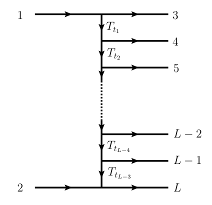
Also in the figure, we have defined the -channel color operator
| (93) |
whose eigenstates are definite -channel exchanges occurring between partons and . In the MR limit the invariants to be inserted into the dipole operators in eq. (35) are approximated (see e.g. eq. (66) of [26]) by their leading rapidity dependence,
| (94) |
where we keep track of the phases, and the notation is chosen so as to explicitly distinguish initial and final state particles.
With this parametrization of momentum invariants, the dipole operator in eq. (35) becomes, in the MR limit,
| (95) | ||||
Note that we have defined here the (unphysical) rapidities and for the initial state particles, which simplifies notation in the first sum on the right-hand side. For later convenience, we also introduce the (unphysical) transverse momenta and . Concentrating on the contents of the square brackets in the exponent, the first (and only rapidity-dependent) term may be rewritten according to
| (96) |
where we have introduced the difference of two consecutive rapidities
| (97) |
while the -channel color operators are defined in eq. (93). A proof of eq. (96) may be found in App. B. One may simplify the coefficients of the other terms by using the color conservation equations
| (98) |
Equation (95) now becomes
| (99) |
as a consequence, the multiparticle dipole operator, in the MR limit, may be written in a factorized form similar to eq. (46), as
| (100) |
where
| (101) | |||||
| (102) | |||||
Eqs. (101, 102) are generalisations to multiparticle amplitudes of the results obtained in the four-point case, expressed in eqs. (47) and (48). As in that example, the non-trivial color matrix contains the dominant contribution in the high-energy limit, consisting of an operator whose eigenstates are definite -channel exchanges. Furthermore, there is a correction which affects the imaginary part of the amplitude starting at NLL, and involving the -channel operator . The factor , proportional to the unit matrix in color space, collects collinear singularities in the form of jet functions for each external particle, as well as terms which only depend upon the quadratic Casimir invariants of individual particles. It is straightforward to check that eqs. (101) and (102) reduce to eqs. (47) and (48) in the special case . Indeed, the non-diagonal factor has only a single -channel exchange with , so that eq. (101) obviously reduces to eq. (47), upon using the fact that the rapidity difference may be expressed as . In eq. (102), one may use the fact that if only two final state particles are present, one has . One then readily recovers eq. (48).
Having derived the form of the dipole operator in MR kinematics, we see that implications regarding Reggeization are directly analogous to the four-point case, and may be stated as follows. If a given -parton hard interaction is dominated by a ladder exchanged in the -channel at leading order, in the MR limit, these automatically Reggeize. By this, we mean that each -channel propagator factor (connecting particles and ) is dressed according to
| (103) |
where is the Regge trajectory of the -channel exchange, involving the appropriate Casimir , and, as before, , using the known form of kinematic invariants in the MR limit [26]. It must of course be stressed again that, as in the case, our approach can only guarantee Reggeization for the singular part of the Regge trajectory.
A further comment is in order, regarding the fact that there are different color operators for each -channel propagator. One could imagine a situation in which these operators might not commute with each other, requiring the use of the Baker-Campbell-Hausdorff formula to compute the action of the Reggeization operator on the hard interaction. This possibility however does not occur. Indeed, the reasoning of App. A, where the possibility of choosing a basis of -channel eigenstates is proven explicitly, shows that the operators always commute,
| (104) |
A simple way to see this here is as follows: one may use the definition of eq. (93) to write
| (105) |
where, without loss of generality, we have taken . One finds then
| (106) |
The right-hand side vanishes, owing to the fact that does not contain for , and one recovers eq. (104). As a consequence, at LL accuracy, where we can neglect the term in the exponent proportional to , we can write the Reggeization operator in a factorized form
| (107) |
In App. A we show that it is always possible to decompose the hard interaction into a colour basis corresponding to an exchange of definite states in the channel. Each channel exchange between, say, the emissions of partons and , is an eigenstate of the corresponding color operator , and its rapidity dependence enters the exponent of the amplitude with the corresponding eigenvalue, so that Reggeization follows. The simplest case is when a single particle species is exchanged in the -channel. One then recovers the well-known Reggeization of leading logarithms in the form of eq. (103). Reggeization, however, is more general than this, as is clear from the structure of eq. (107): in principle, different -channel exchanges may occur, so that different rapidity intervals exponentiate with different eigenvalues.
Computing the four-point amplitude, we found evidence for a breakdown of Reggeization beyond LL order in the imaginary part of the amplitude, and beyond NLL order for the real part. This was due to the term in eq. (47), whose coefficient does not commute in general with the -channel operator. Exactly the same situation occurs in eq. (101), and indeed the same term occurs, which is independent of the number of external partons, as perhaps might be expected for an -channel color structure. We thus observe a corresponding breakdown of Reggeization in the general multiparton case, which is entirely consistent with what happens for . As in that case, this conclusion is robust with respect to possible corrections to the dipole formula arising at three loops.
7 Discussion
In this paper, we have developed an infrared-based approach to the high-energy limit of gauge theory amplitudes, making use of the dipole formula, eq. (35), an explicit ansatz for the all-order infrared singularity structure of fixed-angle scattering amplitudes involving massless partons. We have seen that in the Regge limit the infrared operator , responsible for all soft and collinear singularities in the dipole formula, factors into the product of a color-trivial part, multiplied by the universal high-energy operator of eq. (47), acting on the appropriate hard interaction. If the latter is dominated, as , by the exchange of distinct color states in the -channel, then each such state automatically Reggeizes at leading logarithmic accuracy, at least for the singular part of the amplitude. The infrared-singular part of the renormalized Regge trajectory is given by the function , which is completely determined by the cusp anomalous dimension (and by the -dimensional beta function), and indeed is a well-known function arising in different contexts in perturbative QCD (we note for example that this function assumes a particularly simple form in conformal gauge theories, such as super Yang-Mills theory, as discussed in [51, 105]). These results confirm the calculations of Refs. [40, 41, 38], and they imply that the infrared-singular Regge trajectory is proportional to the quadratic Casimir invariant of the appropriate representation, but is otherwise universal, as was observed in the past in concrete examples. If a number of -channel exchanges are possible – which may occur at different perturbative orders in the hard interaction – then each exchanged state Reggeizes independently.
Approaching the problem of Reggeization with the dipole formula gives insights both on the generality of the phenomenon (as we discussed, every color state giving leading contributions in the -channel Reggeizes at LL accuracy), and on its inherent limitations. We observe that the high-energy operator is diagonal in a -channel basis only at LL level, and is corrected by a phase which depends on the identity of -channel exchanges at NLL. The existence of this phase does not affect Reggeization for the real part of the amplitude at NLL, so that all known results are correctly recovered and extended. The dipole formula, however, is an all-order ansatz, and allows us to explore what happens beyond NLL, and indeed beyond the realm of Regge factorization. We find that Reggeization generically breaks down at NNLL, also for the real part of the amplitude, and we are able to write a completely general form, eq. (86), for the leading Reggeization-breaking operator, which arises at three loops in the exponent. Note, however, that Reggeization for the infrared-singular terms in the amplitude, is preserved in the large- limit, a fact which deserves further investigation.
The fact that the simple form of Regge factorization does not fully describe the high-energy limit of amplitudes is perhaps expected based on the argument that in addition to Regge poles, higher-loop corrections may give rise to Regge cuts [5]. The possible connection between these analytic structures and the violation of the simple Regge pole picture we observed, requires a dedicated study.
Our conclusion concerning Reggeization breaking remains valid even if the dipole formula receives quadrupole corrections at three loops: indeed, possible new contributions to the soft anomalous dimension at the three loops would affect only the single-pole term at NNLL level, not the triple-pole term generated by the Reggeization-breaking operator.
We have also demonstrated, in Sec. 5, that the connection between soft singularities in amplitudes and Reggeization may be exploited to further constrain the soft anomalous dimension matrix. Three-loop corrections to the soft anomalous dimension going beyond the dipole formula have already been shown to be highly constrained by factorization and rescaling symmetry, collinear limits, Bose symmetry and transcendentality [70, 71, 82]. Nevertheless, Ref. [82] provided explicit examples of functions that are consistent with all these constraints. Here, upon considering these functions in the high-energy limit, we have found that they all give rise to super-leading logarithms which conflict with the known behaviour in the Regge limit. Thus, these examples can no longer be considered viable (except if they occur in particular combinations in which the super-leading as well as the leading logarithms cancel out). This gives further support to the validity of the dipole formula beyond two loops. Clearly, however, a proof is still missing.
Finally, we have used the dipole formula to study the high-energy limit of multiparton scattering amplitudes in multi-Regge kinematics. Once again, the dipole formalism proves to be an efficient and appealing way to study the problem: we recover the known form of the amplitude in Regge factorization at LL accuracy, we can readily read off the (divergent part of) the corresponding Regge trajectories, and we can immediately identify the form of Reggeization-breaking operators starting at NNLL level.
In summary, our infrared-based approach offers new insights into the Regge limit, and a particularly clear way of understanding how Reggeization arises, and eventually breaks down. Reggeization, indeed, appears to be an infrared-dominated phenomenon, and one may wonder to what extent the resummation of finite contributions, which start arising at two loops in the Regge trajectory, might be understood from an infrared point of view: in fact, in several cases in the past [125, 126, 68, 127, 51, 128] it was observed that certain classes of infrared-finite contributions are carried along with singularities when these exponentiate. The study of these issues is left for future work.
We believe that our results pave the way for further progress in several directions: corrections to the dipole formula may be further constrained, and perhaps shown to be absent; Reggeization of finite contributions to the amplitude may be studied from an infrared viewpoint; our results may be used to test the breakdown of Reggeization at NNLL and gauge its impact on phenomenology; finally, the infrared singularity structure of amplitudes may be used to study the high-energy limit beyond the realm of Reggeization.
Acknowledgements
We are grateful to Viktor Fadin and Gregory Korchemsky for useful discussions. This work was partly supported by the Research Executive Agency (REA) of the European Union, through the Initial Training Network LHCPhenoNet, under contract PITN-GA-2010-264564, and by MIUR (Italy) under contract 2006020509004. CDW is supported by the STFC Postdoctoral Fellowship “Collider Physics at the LHC”. CDW, CD and VDD are very grateful to the School of Physics and Astronomy at the University of Edinburgh for hospitality on a number of occasions. LM gratefully acknowledges the award of a SUPA Distinguished Visitor Fellowship. VDD, CD and EG thank the KITP, Santa Barbara for hospitality. Finally, VDD and EG thank the GGI, Firenze, for hospitality at the last stages of writing this paper.
Appendix A Reggeization using Clebsch-Gordan coefficients
In Sec. 3.2 we have demonstrated in general how Reggeization arises after decomposing the hard interaction in the Regge limit in a color flow basis consisting of distinct irreducible representations in the channel. These are eigenstates of the Reggeization operator, which contains the quadratic Casimir operator associated with -channel exchanges. It is instructive to see how this works in detail, carrying out the color algebra in full. This is the subject of this appendix.
A.1 Tensor product representations and Clebsch-Gordan coefficients
Scattering amplitudes transform in general as tensors under gauge transformations. In order to lay the ground for our analysis, we start by recalling general facts about tensor product representations and Clebsch-Gordan decompositions.
Consider two vector spaces and transforming in some irreducible representations and of some group . More precisely, let be a basis of . Then the group acts on the basis vectors via
| (108) |
where denotes the representation matrices of in the irreducible representation . The tensor product representation will in general be reducible, and we can decompose into a direct sum
| (109) |
where the sum runs over all irreducible representations of that appear in the decomposition2222 22 If a given irreducible representation appears with multiplicity , we consider each replica separately. of , and is the subspace of that transforms in the irreducible representation . Let be a basis of , which under the group action transforms as
| (110) |
The change of basis is expressed by the unitary transformation whose matrix elements are the Clebsch-Gordan coefficients,
| (111) |
As the change of basis is unitary, the Clebsch-Gordan coefficients must satisfy the relations
| (112) |
as well as
| (113) |
where denotes the irreducible representation complex conjugate to .
Let now be an arbitrary vector in . We can write
| (114) |
Inserting eq. (111) into eq. (114), we immediately see that
| (115) |
and, using the unitarity relations eq. (112) we can invert this relation to obtain
| (116) |
The components of the vector transform under the group action as
| (117) |
Compatibility of these transformations with eq. (115) then implies the relation
| (118) |
or, equivalently, in infinitesimal form,
| (119) |
where denote the generators of the irreducible representation . In the following we will need the equivalent of this relation for the complex conjugated Clebsch-Gordan coefficients . Taking the complex conjugate of the previous equations, and using the fact that the generators are hermitian, we arrive at
| (120) |
Note that this relation is consistent with eq. (113).
A.2 Decomposition of a scattering amplitude in a channel basis
In this section we prove that every scattering amplitude can be decomposed into a channel basis, and that the subamplitudes that appear in this decomposition are eigenstates of the channel colour operators defined in Sec. 6,
| (121) |
Let us consider a scattering of particles, , transforming in the representations , . The scattering amplitude for this process can be seen as a vector in colour space,
| (122) |
The basis vectors transform in the representation of the gauge group2323 23 We consider initial state particles as outgoing antiparticles.,
| (123) |
so that the amplitude transforms as
| (124) |
The colour operators are defined by their action on colour space, according to [113, 114]2424 24 In this section we follow strictly the conventions of [114], which differ slightly from the convention used in the main text.
| (125) |
or equivalently,
| (126) |
Note that in this notation the generators of the representation are just given by . Colour conservation implies that must be a colour singlet, or in other words, is an invariant tensor transforming in the representation . As a consequence, must be annihilated by the generators of the gauge group, leaving us with the usual constraint expressing colour conservation,
| (127) |
Let us now turn to the proof that we can always decompose into a colour basis corresponding to definite channel exchanges. Using eq. (116), one may sequentially multiply representations starting at the top of the ladder in fig. 8, and ending at the bottom. At each step, one eliminates one of the outgoing parton indices in favour of an index associated with the corresponding vertical strut of the ladder, yielding
| (128) | |||||
So far all the manipulations were generic and could have been applied to an arbitrary tensor transforming in the representation . At this stage however we can impose colour conservation in the form of eq. (127) to further constrain the form of the subamplitudes . Acting with the colour operator on the Clebsch-Gordan coefficients, and making repeated use of eq. (120), we arrive at the identity,
| (129) |
The unitarity relations for the Clebsch-Gordan coefficients now imply that this identity can only be fulfilled if the expression inside the square brackets vanishes,
| (130) |
In order to proceed, we have to recall that Schur’s lemma implies that if is an invariant tensor transforming in the representation , i.e.
| (131) |
then must be zero, unless is equivalent to , in which case must be proportional to the identity matrix. Equation (130) is just the infinitesimal form of eq. (131): thus Schur’s lemma implies that
| (132) |
One thus concludes that eq. (128) may be written as
| (133) |
where we defined , , and
| (134) |
Eq. (133) is the desired result: we have written the scattering amplitude as a sum of terms, each characterized by a sequence of irreducible representations , which correspond to the irreducible representations of the states propagating in the channel. Figure 8 gives a diagrammatical representation of a single term in colour flow space.
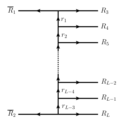
We now want to prove that the colour coefficients , for fixed , are eigenvectors of the channel colour operators defined in eq. (121), and that the eigenvalues are given by the Casimir operators of the representation exchanged in the channel. More precisely,
| (135) |
To prove this, we first act with on the colour coefficient , and we apply the same reasoning as in the derivation of eq. (129), i.e. we make repeated use of eq. (120) to obtain
| (136) | |||||
If we now act a second time with the same operator, we obtain
| (137) | |||||
We conclude that, as desired, is an eigenvector of with eigenvalue . Note that, as this argument is independent of , we have at the same time shown that the operators are simultaneously diagonalizable, and hence always commute
| (138) |
A.3 The Reggeization operator in the -channel basis
Let us now return to the actual problem, and consider the action of the operator of eq. (107) in the high-energy limit, and let us see how this operator acts on the hard amplitude. For simplicity, in this section we concentrate on the case of four-point scattering: the generalisation to multiparticle production is straightforward, since we have shown that all the -channel colour operators commute. The Reggeization operator for a four-point amplitude was given in eq. (50),
| (139) |
We start by decomposing the hard amplitude into a -channel colour basis, as given in eq. (133), writing
| (140) |
Note that in this case simply labels the representation of the state exchanged in the channel. We now act with the Reggeization operator on the hard interaction,
| (141) | |||||
This formula presents explicitly the Reggeization of the singular part of the amplitude. As we already saw each -channel exchange Reggeizes separately, with the exponent being controlled by the corresponding quadratic Casimir.
Appendix B Rapidity-dependent contribution in parton scattering
In this appendix, we prove the result stated in eq. (96), namely that the rapidity-dependent terms in the MR limit of the sum over dipoles formula decompose into a sum over Casimir operators corresponding to definite -channel exchanges, where each is associated with a consecutive rapidity difference.
We start from the left-hand side of eq. (96) and rewrite it as
| (142) |
Next, one may eliminate by using color conservation, eq. (98), to give
| (143) |
where in the second line we have combined the second, third and fourth terms from the previous line. Decomposing the third term in the last line of eq. (143) into three contributions with , and respectively and combining the result with the fourth term gives
| (144) |
where we have interchanged the orders of the summations over and in the final term. Combining this expression with the second term in eq. (143) gives
| (145) |
Note that the contribution from the term in the second term is zero, which allows one to replace the upper limit of the sum over by . One may also relabel and in this term, so that the expression (145) becomes
| (146) |
Combining with the remaining contributions from eq. (143), we find
| (147) |
After interchanging the order of the sums over and in the final term of this expression, we may rewrite eq. (147)
| (148) |
where in the final term one has .
We may now rewrite each rapidity difference in terms of the consecutive differences . That is,
| (149) |
Substituting this in eq. (148) gives
| (150) |
where in the second line we have interchanged the order of summation over and . The coefficient of is
| (151) |
where the right-hand side contains the -channel quadratic Casimir operator defined in eq. (93). This completes the derivation of eq. (96).
References
- (1) P. D. B. Collins, An Introduction to Regge Theory and High-Energy Physics, . Cambridge 1977, 445p.
- (2) D. I. O. R. J. Eden, P. V. Landshoff and J. C. Polkinghorne, The Analytic S-Matrix, . Cambridge 2002, 296p.
- (3) V. N. Gribov, The Theory of Complex Angular Momenta: Gribov Lectures on Theoretical Physics, . Cambridge 2003, 310p.
- (4) M. Gell-Mann and M. L. Goldberger, Elementary particles of conventional field theory as regge poles, Phys. Rev. Lett. 9 (Sep, 1962) 275–277.
- (5) S. Mandelstam, Non-Regge Terms in the Vector-Spinor Theory, Phys. Rev. 137 (1965) B949–B954.
- (6) E. Abers and V. L. Teplitz, Kinematic Constraints, Crossing, and the Reggeization of Scattering Amplitudes, Phys. Rev. 158 (1967) 1365–1376.
- (7) M. T. Grisaru, H. J. Schnitzer, and H.-S. Tsao, Reggeization of yang-mills gauge mesons in theories with a spontaneously broken symmetry, Phys. Rev. Lett. 30 (1973) 811–814.
- (8) M. T. Grisaru, H. J. Schnitzer, and H.-S. Tsao, Reggeization of elementary particles in renormalizable gauge theories - vectors and spinors, Phys. Rev. D8 (1973) 4498–4509.
- (9) M. T. Grisaru, H. J. Schnitzer, and H.-S. Tsao, The Reggeization of elementary particles in renormalizable gauge theories: Scalars, Phys. Rev. D9 (1974) 2864.
- (10) B. M. McCoy and T. T. Wu, Theory of Fermion Exchange in Massive Quantum Electrodynamics at High-Energy. 1, Phys. Rev. D13 (1976) 369–378.
- (11) G. V. Frolov, V. N. Gribov, and L. N. Lipatov, On Regge poles in quantum electrodynamics, Phys. Lett. B31 (1970) 34.
- (12) V. N. Gribov, L. N. Lipatov, and G. V. Frolov, The leading singularity in the j plane in quantum electrodynamics, Sov. J. Nucl. Phys. 12 (1971) 543.
- (13) H. Cheng and T. T. Wu, High-energy collision processes in quantum electrodynamics. i, Phys. Rev. 182 (1969) 1852–1867.
- (14) I. I. Balitsky, L. N. Lipatov, and V. S. Fadin, REGGE PROCESSES IN NONABELIAN GAUGE THEORIES. (IN RUSSIAN), . In *Leningrad 1979, Proceedings, Physics Of Elementary Particles*, Leningrad 1979, 109-149.
- (15) A. V. Bogdan and V. S. Fadin, A proof of the reggeized form of amplitudes with quark exchanges, Nucl. Phys. B740 (2006) 36–57, [hep-ph/0601117].
- (16) L. Tyburski, Reggeization of the Fermion-Fermion Scattering Amplitude in Nonabelian Gauge Theories, Phys. Rev. D13 (1976) 1107.
- (17) L. N. Lipatov, Reggeization of the Vector Meson and the Vacuum Singularity in Nonabelian Gauge Theories, Sov. J. Nucl. Phys. 23 (1976) 338–345.
- (18) A. L. Mason, Radiation Gauge Calculation of High-Energy Scattering Amplitudes, Nucl. Phys. B120 (1977) 275.
- (19) H. Cheng and C. Y. Lo, High-Energy Amplitudes of Yang-Mills Theory in Arbitrary Perturbative Orders. 1, Phys. Rev. D15 (1977) 2959.
- (20) V. S. Fadin, E. A. Kuraev, and L. N. Lipatov, On the Pomeranchuk Singularity in Asymptotically Free Theories, Phys. Lett. B60 (1975) 50–52.
- (21) E. A. Kuraev, L. N. Lipatov, and V. S. Fadin, The Pomeranchuk Singularity in Nonabelian Gauge Theories, Sov. Phys. JETP 45 (1977) 199–204.
- (22) E. A. Kuraev, L. N. Lipatov, and V. S. Fadin, Multi - Reggeon Processes in the Yang-Mills Theory, Sov. Phys. JETP 44 (1976) 443–450.
- (23) A. L. Mason, Factorization and Hence Reggeization in Yang-Mills Theories, Nucl. Phys. B117 (1976) 493.
- (24) A. Sen, Asymptotic Behavior of the Fermion and Gluon Exchange Amplitudes in Massive Quantum Electrodynamics in the Regge Limit, Phys. Rev. D27 (1983) 2997.
- (25) V. S. Fadin and V. E. Sherman, Processes Involving Fermion Exchange in Nonabelian Gauge Theories, Zh. Eksp. Teor. Fiz. 72 (1977) 1640–1658.
- (26) V. Del Duca, An introduction to the perturbative QCD pomeron and to jet physics at large rapidities, hep-ph/9503226.
- (27) J. R. Forshaw and D. A. Ross, Quantum chromodynamics and the pomeron, Cambridge Lect. Notes Phys. 9 (1997) 1–248.
- (28) V. S. Fadin, M. I. Kotsky, and R. Fiore, Gluon Reggeization in QCD in the next-to-leading order, Phys. Lett. B359 (1995) 181–188.
- (29) V. S. Fadin, R. Fiore, and M. I. Kotsky, Gluon Regge trajectory in the two-loop approximation, Phys. Lett. B387 (1996) 593–602, [hep-ph/9605357].
- (30) V. S. Fadin, R. Fiore, and A. Quartarolo, Reggeization of quark quark scattering amplitude in QCD, Phys. Rev. D53 (1996) 2729–2741, [hep-ph/9506432].
- (31) J. Blumlein, V. Ravindran, and W. L. van Neerven, On the gluon Regge trajectory in O(alpha(s)**2), Phys. Rev. D58 (1998) 091502, [hep-ph/9806357].
- (32) V. Del Duca and E. W. N. Glover, The high energy limit of QCD at two loops, JHEP 10 (2001) 035, [hep-ph/0109028].
- (33) A. V. Bogdan, V. Del Duca, V. S. Fadin, and E. W. N. Glover, The quark Regge trajectory at two loops, JHEP 03 (2002) 032, [hep-ph/0201240].
- (34) V. S. Fadin, R. Fiore, M. G. Kozlov, and A. V. Reznichenko, Proof of the multi-Regge form of QCD amplitudes with gluon exchanges in the NLA, Phys. Lett. B639 (2006) 74–81, [hep-ph/0602006].
- (35) G. P. Korchemsky, J. M. Drummond, and E. Sokatchev, Conformal properties of four-gluon planar amplitudes and Wilson loops, Nucl. Phys. B795 (2008) 385–408, [0707.0243].
- (36) J. Bartels, L. N. Lipatov, and A. Sabio Vera, BFKL Pomeron, Reggeized gluons and Bern-Dixon-Smirnov amplitudes, Phys. Rev. D80 (2009) 045002, [0802.2065].
- (37) V. Del Duca and E. W. N. Glover, Testing high-energy factorization beyond the next-to- leading-logarithmic accuracy, JHEP 05 (2008) 056, [0802.4445].
- (38) G. P. Korchemsky, On Near forward high-energy scattering in QCD, Phys. Lett. B325 (1994) 459–466, [hep-ph/9311294].
- (39) M. G. Sotiropoulos and G. F. Sterman, Color exchange in near forward hard elastic scattering, Nucl.Phys. B419 (1994) 59–76, [hep-ph/9310279].
- (40) I. A. Korchemskaya and G. P. Korchemsky, High-energy scattering in QCD and cross singularities of Wilson loops, Nucl. Phys. B437 (1995) 127–162, [hep-ph/9409446].
- (41) I. A. Korchemskaya and G. P. Korchemsky, Evolution equation for gluon Regge trajectory, Phys. Lett. B387 (1996) 346–354, [hep-ph/9607229].
- (42) T. Kucs, QCD resummation techniques, hep-ph/0403023. Ph.D. Thesis (Advisor: George Sterman).
- (43) Y. Dokshitzer and G. Marchesini, Soft gluons at large angles in hadron collisions, JHEP 0601 (2006) 007, [hep-ph/0509078].
- (44) I. Balitsky, High-energy QCD and Wilson lines, hep-ph/0101042. To be published in the Boris Ioffe Festschrift: At the Frontier of Particle Physics / Handbook of QCD. Edited by M. Shifman, Singapore, World, Scientific, 2001.
- (45) G. Korchemsky, Asymptotics of the Altarelli-Parisi-Lipatov Evolution Kernels of Parton Distributions, Mod.Phys.Lett. A4 (1989) 1257–1276.
- (46) G. Korchemsky, Sudakov form-factor in QCD, Phys.Lett. B220 (1989) 629.
- (47) G. Korchemsky and A. Radyushkin, Renormalization of the Wilson Loops Beyond the Leading Order, Nucl.Phys. B283 (1987) 342–364.
- (48) S. Ivanov, G. Korchemsky, and A. Radyushkin, Infrared Asymptotics of Perturbative QCD: Contour Gauges, Yad.Fiz. 44 (1986) 230–240.
- (49) G. Korchemsky and A. Radyushkin, Loop Space Formalism and Renormalization Group for the Infrared Asymptotics of QCD, Phys.Lett. B171 (1986) 459–467.
- (50) I. I. Balitsky and L. N. Lipatov, The Pomeranchuk Singularity in Quantum Chromodynamics, Sov. J. Nucl. Phys. 28 (1978) 822–829.
- (51) Z. Bern, L. J. Dixon, and V. A. Smirnov, Iteration of planar amplitudes in maximally supersymmetric Yang-Mills theory at three loops and beyond, Phys. Rev. D72 (2005) 085001, [hep-th/0505205].
- (52) V. Del Duca, C. Duhr, and E. W. N. Glover, Iterated amplitudes in the high-energy limit, JHEP 12 (2008) 097, [0809.1822].
- (53) R. C. Brower, H. Nastase, H. J. Schnitzer, and C.-I. Tan, Implications of multi-Regge limits for the Bern-Dixon-Smirnov conjecture, Nucl.Phys. B814 (2009) 293–326, [0801.3891].
- (54) R. C. Brower, H. Nastase, H. J. Schnitzer, and C.-I. Tan, Analyticity for Multi-Regge Limits of the Bern-Dixon-Smirnov Amplitudes, Nucl.Phys. B822 (2009) 301–347, [0809.1632].
- (55) V. Del Duca, C. Duhr, and V. A. Smirnov, An Analytic Result for the Two-Loop Hexagon Wilson Loop in N = 4 SYM, JHEP 03 (2010) 099, [0911.5332].
- (56) V. Del Duca, C. Duhr, and V. A. Smirnov, The Two-Loop Hexagon Wilson Loop in N = 4 SYM, JHEP 05 (2010) 084, [1003.1702].
- (57) V. Del Duca, C. Duhr, and V. A. Smirnov, A Two-Loop Octagon Wilson Loop in N = 4 SYM, JHEP 09 (2010) 015, [1006.4127].
- (58) L. F. Alday and J. M. Maldacena, Gluon scattering amplitudes at strong coupling, JHEP 06 (2007) 064, [0705.0303].
- (59) A. Brandhuber, P. Heslop, and G. Travaglini, MHV Amplitudes in N=4 Super Yang-Mills and Wilson Loops, Nucl. Phys. B794 (2008) 231–243, [0707.1153].
- (60) V. Del Duca, C. Duhr, E. Gardi, L. Magnea, and C. D. White, An infrared approach to Reggeization, 1108.5947. * Temporary entry *.
- (61) J. Grammer, G. and D. Yennie, Improved treatment for the infrared divergence problem in quantum electrodynamics, Phys.Rev. D8 (1973) 4332–4344.
- (62) A. H. Mueller, On the asymptotic behavior of the Sudakov form-factor, Phys. Rev. D20 (1979) 2037.
- (63) J. C. Collins, Algorithm to compute corrections to the Sudakov form factor, Phys. Rev. D22 (1980) 1478.
- (64) A. Sen, Asymptotic behavior of the Sudakov form-factor in QCD, Phys. Rev. D24 (1981) 3281.
- (65) A. Sen, Asymptotic Behavior of the Wide Angle On-Shell Quark Scattering Amplitudes in Nonabelian Gauge Theories, Phys. Rev. D28 (1983) 860.
- (66) J. Gatheral, Exponentiation of eikonal cross sections in nonabelian gauge theories, Phys.Lett. B133 (1983) 90.
- (67) J. Frenkel and J. Taylor, Nonabelian eikonal exponentiation, Nucl.Phys. B246 (1984) 231.
- (68) L. Magnea and G. F. Sterman, Analytic continuation of the Sudakov form-factor in QCD, Phys.Rev. D42 (1990) 4222–4227.
- (69) T. Becher and M. Neubert, Infrared singularities of scattering amplitudes in perturbative QCD, Phys. Rev. Lett. 102 (2009) 162001, [0901.0722].
- (70) E. Gardi and L. Magnea, Factorization constraints for soft anomalous dimensions in QCD scattering amplitudes, JHEP 03 (2009) 079, [0901.1091].
- (71) T. Becher and M. Neubert, On the Structure of Infrared Singularities of Gauge-Theory Amplitudes, JHEP 06 (2009) 081, [0903.1126].
- (72) E. Gardi and L. Magnea, Infrared singularities in QCD amplitudes, Nuovo Cim. C32N5-6 (2009) 137–157, [0908.3273].
- (73) N. Kidonakis, Two-loop soft anomalous dimensions and NNLL resummation for heavy quark production, Phys. Rev. Lett. 102 (2009) 232003, [0903.2561].
- (74) A. Mitov, G. Sterman, and I. Sung, The Massive Soft Anomalous Dimension Matrix at Two Loops, Phys. Rev. D79 (2009) 094015, [0903.3241].
- (75) T. Becher and M. Neubert, Infrared singularities of QCD amplitudes with massive partons, Phys. Rev. D79 (2009) 125004, [0904.1021].
- (76) M. Beneke, P. Falgari, and C. Schwinn, Soft radiation in heavy-particle pair production: All-order colour structure and two-loop anomalous dimension, Nucl.Phys. B828 (2010) 69–101, [0907.1443].
- (77) M. Czakon, A. Mitov, and G. F. Sterman, Threshold Resummation for Top-Pair Hadroproduction to Next-to-Next-to-Leading Log, Phys.Rev. D80 (2009) 074017, [0907.1790].
- (78) A. Ferroglia, M. Neubert, B. D. Pecjak, and L. L. Yang, Two-loop divergences of scattering amplitudes with massive partons, Phys.Rev.Lett. 103 (2009) 201601, [0907.4791].
- (79) A. Ferroglia, M. Neubert, B. D. Pecjak, and L. L. Yang, Two-loop divergences of massive scattering amplitudes in non-abelian gauge theories, JHEP 0911 (2009) 062, [0908.3676].
- (80) J.-y. Chiu, A. Fuhrer, R. Kelley, and A. V. Manohar, Factorization Structure of Gauge Theory Amplitudes and Application to Hard Scattering Processes at the LHC, Phys.Rev. D80 (2009) 094013, [0909.0012].
- (81) A. Mitov, G. F. Sterman, and I. Sung, Computation of the Soft Anomalous Dimension Matrix in Coordinate Space, Phys.Rev. D82 (2010) 034020, [1005.4646].
- (82) L. J. Dixon, E. Gardi, and L. Magnea, On soft singularities at three loops and beyond, JHEP 02 (2010) 081, [0910.3653].
- (83) V. Del Duca, Equivalence of the Parke-Taylor and the Fadin-Kuraev- Lipatov amplitudes in the high-energy limit, Phys. Rev. D52 (1995) 1527–1534, [hep-ph/9503340].
- (84) V. Del Duca, Next-to-leading corrections to the BFKL equation, hep-ph/9605404.
- (85) L. N. Lipatov, High-energy scattering in QCD and in quantum gravity and two-dimensional field theories, Nucl. Phys. B365 (1991) 614–632.
- (86) V. S. Fadin and L. N. Lipatov, High-Energy Production of Gluons in a QuasimultiRegge Kinematics, JETP Lett. 49 (1989) 352.
- (87) V. Del Duca, Real next-to-leading corrections to the multigluon amplitudes in the helicity formalism, Phys. Rev. D54 (1996) 989–1009, [hep-ph/9601211].
- (88) V. S. Fadin and L. N. Lipatov, Next-to-leading Corrections to the BFKL Equation From the Gluon and Quark Production, Nucl. Phys. B477 (1996) 767–808, [hep-ph/9602287].
- (89) V. Del Duca, Quark-antiquark contribution to the multigluon amplitudes in the helicity formalism, Phys. Rev. D54 (1996) 4474–4482, [hep-ph/9604250].
- (90) V. S. Fadin and L. N. Lipatov, Radiative corrections to QCD scattering amplitudes in a multi - Regge kinematics, Nucl. Phys. B406 (1993) 259–292.
- (91) V. S. Fadin, R. Fiore, and A. Quartarolo, Quark contribution to the reggeon - reggeon - gluon vertex in QCD, Phys. Rev. D50 (1994) 5893–5901, [hep-th/9405127].
- (92) V. S. Fadin, R. Fiore, and M. I. Kotsky, Gribov’s theorem on soft emission and the Reggeon-Reggeon- gluon vertex at small transverse momentum, Phys. Lett. B389 (1996) 737–741, [hep-ph/9608229].
- (93) V. Del Duca and C. R. Schmidt, Virtual next-to-leading corrections to the Lipatov vertex, Phys. Rev. D59 (1999) 074004, [hep-ph/9810215].
- (94) Z. Bern, V. Del Duca, and C. R. Schmidt, The infrared behavior of one-loop gluon amplitudes at next-to-next-to-leading order, Phys. Lett. B445 (1998) 168–177, [hep-ph/9810409].
- (95) V. S. Fadin and L. N. Lipatov, BFKL pomeron in the next-to-leading approximation, Phys. Lett. B429 (1998) 127–134, [hep-ph/9802290].
- (96) G. Camici and M. Ciafaloni, Irreducible part of the next-to-leading BFKL kernel, Phys. Lett. B412 (1997) 396–406, [hep-ph/9707390].
- (97) M. Ciafaloni and G. Camici, Energy scale(s) and next-to-leading BFKL equation, Phys. Lett. B430 (1998) 349–354, [hep-ph/9803389].
- (98) M. Gell-Mann, M. L. Goldberger, F. E. Low, E. Marx, and F. Zachariasen, Elementary particles of conventional field theory as regge poles. iii, Phys. Rev. 133 (Jan, 1964) B145–B160.
- (99) M. Gell-Mann, M. L. Goldberger, F. E. Low, V. Singh, and F. Zachariasen, Elementary particles of conventional field theory as regge poles. iv, Phys. Rev. 133 (Jan, 1964) B161–B174.
- (100) Z. Bern, J. Carrasco, L. J. Dixon, H. Johansson, and R. Roiban, Manifest Ultraviolet Behavior for the Three-Loop Four-Point Amplitude of N=8 Supergravity, Phys.Rev. D78 (2008) 105019, [0808.4112].
- (101) S. M. Aybat, L. J. Dixon, and G. F. Sterman, The two-loop soft anomalous dimension matrix and resummation at next-to-next-to leading pole, Phys. Rev. D74 (2006) 074004, [hep-ph/0607309].
- (102) G. F. Sterman, Partons, factorization and resummation, hep-ph/9606312.
- (103) N. Kidonakis, G. Oderda, and G. F. Sterman, Evolution of color exchange in QCD hard scattering, Nucl. Phys. B531 (1998) 365–402, [hep-ph/9803241].
- (104) G. F. Sterman and M. E. Tejeda-Yeomans, Multi-loop amplitudes and resummation, Phys. Lett. B552 (2003) 48–56, [hep-ph/0210130].
- (105) L. J. Dixon, L. Magnea, and G. F. Sterman, Universal structure of subleading infrared poles in gauge theory amplitudes, JHEP 08 (2008) 022, [0805.3515].
- (106) S. G. Naculich and H. J. Schnitzer, Eikonal methods applied to gravitational scattering amplitudes, JHEP 05 (2011) 087, [1101.1524].
- (107) C. D. White, Factorization Properties of Soft Graviton Amplitudes, JHEP 05 (2011) 060, [1103.2981].
- (108) R. Akhoury, R. Saotome, and G. Sterman, Collinear and Soft Divergences in Perturbative Quantum Gravity, 1109.0270. * Temporary entry *.
- (109) A. M. Polyakov, Gauge Fields as Rings of Glue, Nucl. Phys. B164 (1980) 171–188.
- (110) I. Y. Arefeva, Quantun Contour Field Equations, Phys. Lett. B93 (1980) 347–353.
- (111) V. S. Dotsenko and S. N. Vergeles, Renormalizability of Phase Factors in the Nonabelian Gauge Theory, Nucl. Phys. B169 (1980) 527.
- (112) R. A. Brandt, F. Neri, and M.-a. Sato, Renormalization of Loop Functions for All Loops, Phys. Rev. D24 (1981) 879.
- (113) A. Bassetto, M. Ciafaloni, and G. Marchesini, Jet Structure and Infrared Sensitive Quantities in Perturbative QCD, Phys.Rept. 100 (1983) 201–272.
- (114) S. Catani and M. H. Seymour, A general algorithm for calculating jet cross sections in NLO QCD, Nucl. Phys. B485 (1997) 291–419, [hep-ph/9605323].
- (115) S. Moch, J. Vermaseren, and A. Vogt, The Three loop splitting functions in QCD: The Nonsinglet case, Nucl.Phys. B688 (2004) 101–134, [hep-ph/0403192].
- (116) E. Gardi, E. Laenen, G. Stavenga, and C. D. White, Webs in multiparton scattering using the replica trick, JHEP 1011 (2010) 155, [1008.0098].
- (117) A. Mitov, G. Sterman, and I. Sung, Diagrammatic Exponentiation for Products of Wilson Lines, Phys.Rev. D82 (2010) 096010, [1008.0099].
- (118) M. Sjodahl, Color evolution of 2 3 processes, JHEP 0812 (2008) 083, [0807.0555].
- (119) M. Anselmino, E. Predazzi, S. Ekelin, S. Fredriksson, and D. Lichtenberg, Diquarks, Rev.Mod.Phys. 65 (1993) 1199–1234.
- (120) T. Han, I. Lewis, and T. McElmurry, QCD Corrections to Scalar Diquark Production at Hadron Colliders, JHEP 1001 (2010) 123, [0909.2666].
- (121) W. Magnus, On the exponential solution of differential equations for a linear operator, Comm. Pure Appl. Math 7 (1954) 649.
- (122) J. Bartels and C. Bontus, An estimate of twist-four contributions at small x(B) and low Q**2, Phys. Rev. D61 (2000) 034009, [hep-ph/9906308].
- (123) S. Marzani, R. D. Ball, P. Falgari, and S. Forte, BFKL at next-to-next-to-leading order, Nucl.Phys. B783 (2007) 143–175, [0704.2404].
- (124) S. Marzani, R. Ball, P. Falgari, and S. Forte, BFKL at NNLO, 0708.3994.
- (125) G. Parisi, Summing Large Perturbative Corrections in QCD, Phys.Lett. B90 (1980) 295.
- (126) G. F. Sterman, Summation of Large Corrections to Short Distance Hadronic Cross-Sections, Nucl.Phys. B281 (1987) 310.
- (127) T. O. Eynck, E. Laenen, and L. Magnea, Exponentiation of the Drell-Yan cross-section near partonic threshold in the DIS and MS-bar schemes, JHEP 0306 (2003) 057, [hep-ph/0305179].
- (128) V. Ahrens, T. Becher, M. Neubert, and L. L. Yang, Origin of the Large Perturbative Corrections to Higgs Production at Hadron Colliders, Phys.Rev. D79 (2009) 033013, [0808.3008].