Floer cohomology in the mirror of the projective plane and a binodal cubic curve
Abstract.
We construct a family of Lagrangian submanifolds in the Landau–Ginzburg mirror to the projective plane equipped with a binodal cubic curve as anticanonical divisor. These objects correspond under mirror symmetry to the powers of the twisting sheaf , and hence their Floer cohomology groups form an algebra isomorphic to the homogeneous coordinate ring. An interesting feature is the presence of a singular torus fibration on the mirror, of which the Lagrangians are sections. This gives rise to a distinguished basis of the Floer cohomology and the homogeneous coordinate ring parametrized by fractional integral points in the singular affine structure on the base of the torus fibration. The algebra structure on the Floer cohomology is computed using the symplectic techniques of Lefschetz fibrations and the TQFT counting sections of such fibrations. We also show that our results agree with the tropical analog proposed by Abouzaid–Gross–Siebert. Extensions to a restricted class of singular affine manifolds and to mirrors of the complements of components of the anticanonical divisor are discussed.
1. Introduction
This article is concerned with a case of mirror symmetry relating the algebraic geometry of a Fano manifold to the symplectic geometry of a Landau–Ginzburg model. The Fano manifold is the projective plane with homogeneous coordinates , and additionally we choose as anticanonical divisor , the union of a conic and a line (a binodal cubic curve). According to Auroux [7], the mirror of this pair is the Landau–Ginzburg model
| (1) |
The function is known as the superpotential. This example is interesting in the context of the Strominger-Yau-Zaslow picture of mirror symmetry [42] in terms of dual torus fibrations, since the spaces and admit special Lagrangian torus fibrations with a singularity. The presence of singularities in the torus fibration is known to make the mirror duality vastly more complicated, but in this article we develop techniques to deal with it in the above case (and other cases with similar properties, see §6).
1.1. Summary of results
The piece of symplectic geometry in the Landau–Ginzburg model we study is the Floer cohomology of Lagrangian submanifolds, while on the mirror side we consider the cohomology of the coherent sheaves . We construct a symplectic manifold , that serves as our symplectic model for , and a collection of Lagrangian submanifolds in that is mirror to the collection . The constructions of and are based on the SYZ picture of mirror symmetry in terms of torus fibrations and affine manifolds, and also use the theory of Lefschetz fibrations. The manifold carries two fibrations: one is a fibration over a singular affine manifold whose fibers are Lagrangian tori, while the other is a Lefschetz fibration whose fibers are symplectic submanifolds. See section 3 for the definitions.
To state the main result, let , and choose a basis of . Thus is the homogeneous coordinate ring of . The Floer cohomology of two Lagrangian submanifolds is a -graded -vector space denoted .
Theorem 1.1.
For each and , there is an isomorphism
| (2) |
carrying the basis of intersection points to the basis of consisting of the polynomials of the form
| (3) |
(where we require ). The system of isomorphisms intertwines the Floer triangle product
| (4) |
and the product of polynomials .
Let us remark on the formulation of the theorem. From the construction of the Lagrangians it is easy to count the number of intersection points and show that the map exists as an isomorphism of vector spaces. Such a map exists for any choice of basis of . The last statement equating Floer triangle products and the products of polynomials is the nontrivial bit that ties the choices together and shows that we have chosen the right basis for .
This basis we obtain is related to the choice of divisor , as it consists of monomials in the defining section of , the defining section of , and the homogeneous variables or (but not both and in the same monomial). Another point of view has to do with the fact that the ring of functions on is a cluster algebra [12]. There are two triples of homogeneous forms on , and , which are related by the so-called exchange relation , and our basis consists of sections that are monomials in either triple.
For the proof of this theorem, the majority of our technical efforts are aimed at computing the Floer triangle product. This occupies section 4. At this point in the argument, the picture of as a Lefschetz fibration is the focus. The holomorphic triangles we need to find can be represented as sections of this Lefschetz fibration. The problem of counting sections of Lefschetz fibrations has a TQFT-type structure, developed by Seidel. This structure, where one breaks a given problem into simpler ones by degenerating the base of the Lefschetz fibration, provides the basis of our technique.
There are several variations on Theorem 1.1 that are accessible using the same holomorphic curve analysis. We consider the complement of (some components of) the anticanonical divisor in , and on the Landau–Ginzburg side, we must change the superpotential and consider a certain form of wrapped Floer cohomology. Our techniques allow us to treat three cases:
- (1)
the mirror of ,
- (2)
the mirror of , and
- (3)
the mirror of .
In each case the mirror space is the same manifold , and the Lagrangians mirror to line bundles are the same , but in each case there is a different prescription for wrapping the Lagrangian submanifolds. The first two cases require “partially wrapped” Floer cohomology, while the third uses the more standard “fully wrapped” Floer cohomology. In each case we denote wrapped Floer cohomology by . Let , , or , and let . The space consists of rational functions in the variables that are regular on and have degree . The wrapped version of Theorem 1.1 is as follows (see §7)
Theorem 1.2.
For and , there is an isomorphism
| (5) |
carrying a certain distinguished basis of to the basis of consisting of rational functions of the form
| (6) |
where the exponents and are restricted to those values which actually give elements of . The system of isomorphisms intertwines the Floer triangle product on wrapped Floer cohomology and the product of rational functions .
While our holomorphic triangle counts use the structure of a Lefschetz fibration on , we can also study the geometry of the as a Lagrangian torus fibration over the base affine manifold . One of the expectations of SYZ philosophy is that much of the geometry of the space can be seen tropically, in terms of the geometry of the affine base .
In fact, this is how we arrive at the construction of the manifold . In section 2, we construct a tropicalization of the fiber of the superpotential over a large positive real value, with respect to a torus fibration on the manifold with a single singularity. This gives a tropical curve in the base of our torus fibration. It bounds a compact region in the base, which agrees with the affine base of the torus fibration on . The purpose of this section is to motivate the use of the singular affine manifold as the basis for our main symplectic constructions in section 3.
We also are able to verify a conjectural tropical description of Floer cohomology in the cases we study. This description comes from a recent proposal of Abouzaid, Gross and Siebert for a tropical Fukaya category associated to a singular affine manifold. The Lagrangian submanifolds are taken to be sections of the torus fibration, but all we see of them tropically are their intersection points, which map to fractional integral points of the affine manifold . The Floer triangle product corresponds to a “tropical triangle product” counting certain tropical curves in joining the fractional integral points. Since we do not say anything about degenerating holomorphic polygons to tropical ones, we merely verify the equivalence by matching bases and computing on both sides. See section 5 for the precise definitions of the terms.
Theorem 1.3.
There is a bijection between the basis of intersection points for and the set of -integral points of the affine manifold . Under this bijection, the counts of pseudo-holomorphic triangles contributing to the Floer triangle product are equal to counts of tropical curves in joining -integral points.
The techniques developed in this article apply to a larger but still restricted class of –dimensional singular affine manifolds, where the main restriction is that all singularities have parallel monodromy-invariant directions. The generalization to these types of manifolds is discussed in 6.
1.2. Context and related work
1.2.1. Manifolds with effective anticanonical divisor and Landau–Ginzburg models
The class of spaces originally considered in mirror symmetry were Calabi–Yau manifolds. Roughly speaking, the mirror to a compact Calabi–Yau manifold is another compact Calabi–Yau manifold of the same dimension. For example, it is in this context that we have the equivalence, discovered by Candelas–de la Ossa–Green–Parkes [10] and proven mathematically by Givental [15] and Lian–Liu–Yau [33], between the Gromov–Witten theory of the quintic threefold and the theory of period integrals on a family of Calabi–Yau threefolds known as “mirror quintics.” However, mirror symmetry can be considered for other classes of manifolds such as manifolds of general type ( ample), for which a proposal has recently been made by Kapustin–Katzarkov–Orlov–Yotov [27], and (our present concern) manifolds with an effective anticanonical divisor. In both of these latter cases the mirror is not a manifold of the same class.
Let be an –dimensional Kähler manifold with an effective anticanonical divisor . We regard as part of the data, and write for the pair. We also choose a meromorphic –form with no zeros and polar locus equal to . According to Hori–Vafa [25] and Givental, the mirror to is a Landau–Ginzburg model , consisting of a Kähler manifold , together with a holomorphic function , called the superpotential.
The mirrors of toric Fano manifolds were derived by Hori–Vafa [25, §5.3] based on physical considerations. Let be an –dimensional toric Fano manifold, and let be the complement of the open torus orbit. The mirror is then with a superpotential given by a sum of monomials corresponding to the one-dimensional cones in the fan for . Choose a polarization with corresponding moment polytope , a lattice polytope in . For each facet of , let to be the primitive integer inward-pointing normal vector, and let be such that is the equation for the hyperplane containing . Then mirror Landau-Ginzburg model is given by
| (7) |
where is a monomial in multi-index notation.
In the case where is toric but not necessarily Fano, a similar formula for the mirror superpotential is expected to hold, which differs by the addition of “higher order” terms [14, Theorems 4.5, 4.6].
The Hori–Vafa formula contains the case of the projective plane with the toric boundary as anticanonical divisor. If denote homogeneous coordinates, then can be taken to be , the union of the coordinate lines. We then have
| (8) |
where is a parameter that measures the cohomology class of the Kähler form on .
The example with which we are primarily concerned in this paper is also , but with respect to a different, non-toric boundary divisor. Consider the meromorphic –form , whose polar locus is the binodal cubic curve . Thus is the union of a conic and a line . The construction of the mirror to this pair is due to Auroux [7], and we have
| (9) |
A direct computation shows that both superpotentials and have the same critical values
| (10) |
It is also easy to see that any regular fiber of is a three-times-punctured elliptic curve, while any regular fiber is a twice-punctured elliptic curve. This is an example of the general expectation that partially smoothing the anticanonical divisor corresponds to partially compactifying the total space of the Landau–Ginzburg model.
1.2.2. Torus fibrations and affine manifolds
One justification that (8)–(9) are appropriate mirrors is found in the Strominger–Yau–Zaslow proposal, which expresses mirror symmetry geometrically in terms of dual torus fibrations, a relationship also known as T–duality. Ideally, one would expect that and are dual special Lagrangian torus fibrations over the same base . When this holds true, the mirror can be constructed as the complexified moduli space of special Lagrangian fibers of [35], [23],[7, §2]. The superpotential can be expressed as a function on this moduli space counting Maslov index two disks with boundary on the Lagrangian fibers of , weighted by symplectic area and the holonomy of a local system [7].
For our purposes, a Lagrangian submanifold of a Kähler manifold with meromorphic –form is called special of phase if . Obviously this only makes sense in the complement of the polar locus . The infinitesimal deformations of a special Lagrangian submanifold are given by , and are unobstructed [35]. If is a torus, is an –dimensional space, and in good cases the special Lagrangian deformations of are all disjoint, and form the fibers of a fibration , where is the global parameter space for the deformations of .
Assuming this, define the complexified moduli space of deformations of to be the space consisting of pairs , where is a special Lagrangian deformation of , and is a local system on . There is an obvious projection given by forgetting the local system. The fiber is the space of local systems on the given torus , which is precisely the dual torus . In this sense, the fibrations and are dual torus fibrations, and the SYZ proposal can be taken to mean that the mirror is precisely this complexified moduli space: . The picture is completed by showing that naturally admits a complex structure , a Kähler form , and a holomorphic –form . One finds that is constructed from , while is constructed from , thus expressing the interchange of symplectic and complex structures between the two sides of the mirror pair. For details we refer the reader to [23],[7, §2].
However, this picture of mirror symmetry cannot be correct as stated, as it quickly hits upon a major stumbling block: the presence of singular fibers in the original fibration . These singularities make it impossible to obtain the mirror manifold by a fiberwise dualization, and generate “quantum corrections” that complicate the T-duality prescription. Attempts to overcome this difficulty led to the work of Kontsevich and Soibelman [30, 31] and Gross and Siebert [19, 20, 21] that implements the SYZ program in an algebro-geometric context. In the case of K3 surfaces, the work of Fukaya–Oh–Ohta–Ono [13] relates this problem to the wall–crossing of holomorphic disk moduli spaces. It is also this difficulty which motivates us to consider the case of relative to a binodal cubic curve, where the simplest type of singularity arises.
In the case of with effective anticanonical divisor , we can see these corrections in action if we include the superpotential into the SYZ picture. As is to be a function on , which is naively , assigns a complex number to each pair . This number is a count of holomorphic disks with boundary on , of Maslov index , weighted by symplectic area and the holonomy of :
| (11) |
where is the count of holomorphic disks in the class passing through a general point of .
In the toric case, , and we the special Lagrangian torus fibration is simply the map , . This fibration has no singularities, and the above prescriptions work as stated. In the toric Fano case, we recover the Hori–Vafa superpotential (7).
In the case of with the non-toric divisor , the torus fibration has one singular fiber, which is a pinched torus (a focus-focus singularity). The above prescription breaks down: one finds that the superpotential counting disks is not a continuous function on the moduli space of special Lagrangians. This leads one to redefine by breaking it into pieces and re-gluing so as to make continuous, leading to (9) [7]. We find that also admits a special Lagrangian torus fibration with one singular fiber.
In general, the structure of a special Lagrangian torus fibration yields the structure of an tropical affine manifold on the base . This is a manifold with a distinguished collection of affine coordinate charts, such that the transition maps between affine coordinate charts lie in , the group of affine linear transformations with integral linear part. When singular fibers are present in the torus fibration, we simply regard the affine structure as being undefined at the singular fibers and call the resulting structure on the base a singular tropical affine manifold. In fact, the base inherits two affine structures, one from the symplectic form , and one from the holomorphic –form . The former is called the symplectic affine structure, and the latter is called the complex affine structure.
Let us recall briefly how the local affine coordinates are defined. For the symplectic affine structure, we choose a collection of loops that form a basis of . Let be a tangent vector to the base, and take be any vector field along which lifts it. Then
| (12) |
defines a -form on : since is Lagrangian, the integrand is independent of the lift , and only depends on the class of in homology. In fact, the collection forms a basis of , and there is a coordinate system such that ; these are the affine coordinates. This definition actually shows us that there is a canonical isomorphism . This isomorphism induces an integral structure on : , which is preserved by all transition functions between coordinate charts. Thus, when an affine manifold arises as the base of a torus fibration in this way, the structural group is reduced to , the group of affine linear transformations with integral linear part.
The complex affine structure follows exactly the same pattern, only that we take to be –cycles forming a basis of , and in place of we use . Now we have an isomorphism , or equivalently , which induces the integral structure.
The affine manifolds we consider in this article satisfy a stronger integrality condition, which requires the translational part of each transition function to be integral as well. We use the term integral affine manifold to denote an affine manifold whose structural group has been reduced to . Such affine manifolds are “defined over ” and have an intrinsically defined lattice of integral points.
For an integral affine manifold, it makes sense to speak of tropical subvarieties. These are certain piecewise linear complexes contained in , which in some way correspond to holomorphic or Lagrangian submanifolds of the total space of the torus fibration. Tropical geometry has played a role in much work on mirror symmetry, particularly in the program of Gross and Siebert, and closer to this paper, in Abouzaid’s work on mirror symmetry for toric varieties [1, 3]. See [26] for a general introduction to tropical geometry. Though most of the methods in this paper are explicitly symplectic, tropical geometry appears in section 2, where we compute the tropicalization of the fiber of the superpotential, and in section 5, where a class of tropical curves corresponding to holomorphic polygons is considered.
1.2.3. Homological mirror symmetry
The results on Floer cohomology that we prove fall under the heading homological mirror symmetry (HMS) [28], which holds that mirror symmetry can be interpreted as an equivalence of categories associated to the complex or algebraic geometry of , and the symplectic geometry of , and vice–versa. The categories which are appropriate depend somewhat on the situation, so let us focus on the case of the a manifold with anticanonical divisor , and its mirror Landau–Ginzburg model .
Associated to , we take the derived category of coherent sheaves , while to we associate a Fukaya-type A∞-category whose objects are certain Lagrangian submanifolds of , morphism spaces are generated by intersection points, and the A∞ product structures are defined by counting pseudo-holomorphic polygons with boundary on a collection of Lagrangian submanifolds. Our main reference for Floer cohomology and Fukaya categories is the book of Seidel [41].
The superpotential enters the definition of by restricting the class of objects to what are termed admissible Lagrangian submanifolds. In this paper, it will mean that we allow Lagrangian submanifolds that are not closed but which have boundary on a reducible hypersurface whose components are defined by setting one term of the superpotential equal to a constant. Historically, there have been several attempts to formulate the notion of admissibility. Originally, Kontsevich [29] and Hori–Iqbal–Vafa [24] considered those Lagrangian submanifolds , not necessarily compact, which outside of a compact subset are invariant with respect to the gradient flow of . An alternative formulation, due to Abouzaid [1, 3], trades the non-compact end for a boundary on a fiber of , together with the condition that, near the boundary, the maps by to a curve in . A further reformulation, which is more directly related to the SYZ picture, replaces the fiber with the union of hypersurfaces , where is the term in the superpotential (11) corresponding to the class , and admissibility means that near , maps by to a curve in . The admissibility condition we use in this paper is closest to this last formulation.
With these definitions, homological mirror symmetry amounts to an equivalence of categories , where denotes the split-closed derived category of the A∞–category. This piece of mirror symmetry has been addressed many times [9, 8, 37, 1, 3, 11], including results for the projective plane and its toric mirror.
However, in this article, we emphasize less the equivalences of categories themselves, and focus more on geometric structures which arise from a combination of the HMS equivalence with the SYZ picture. When dual torus fibrations are present on the manifolds in a mirror pair, one expects the correspondence between coherent sheaves and Lagrangian submanifolds to be expressible in terms of a Fourier–Mukai transform with respect to the torus fibration [32]. In particular, Lagrangian submanifolds that are sections of the torus fibration correspond to line bundles on , and the Lagrangians we consider are of this type.
In this context, our Theorem 1.1 can be interpreted as yielding an embedding (at the cohomology level) of the subcategory of containing the Lagrangians into .
1.2.4. Distinguished bases
The combination of SYZ and HMS also gives rise to the expectation that, at least in favorable situations, the spaces of sections of coherent sheaves on can be equipped with distinguished bases. Suppose that is a functor implementing the HMS equivalence. Let be two objects of the Fukaya category supported by transversely intersecting Lagrangian submanifolds. Then
| (13) |
Suppose furthermore that the differential on the Floer cochain complex vanishes, so that . As is defined to have a basis in bijection with the set of intersection points , one obtains a basis of parametrized by the same set via the above isomorphisms. If is some sheaf of interest, and by convenient choice of and we can ensure and , then we will obtain a basis for .
When and are mirror dual elliptic curves, this phenomenon is evident in the work of Polishchuk–Zaslow [36] and especially M. Gross [6, Ch. 8]. Both and may be written as special Lagrangian -fibrations over the same base . The base has an integral affine structure as . The Lagrangians are sections of this torus fibration with slope , and their intersection points project precisely to the fractional integral points of the base .
| (14) |
Under HMS, we obtain and . the basis of intersection points corresponds to a basis of consisting of theta functions.
Another illustration is the case of toric varieties and their mirror Landau-Ginzburg models [1, 3]. In this case, Abouzaid constructs a family of Lagrangian submanifolds mirror to the powers of the ample line bundle . These Lagrangian submanifolds are topologically discs with boundary on a level set of the superpotential, for some . For , the Floer complex is concentrated in degree zero. Hence
| (15) |
The basis of intersection points corresponds to the basis of characters of the algebraic torus which appear in the -module . The same formula (14) is valid in the case of toric varieties, where the base is the moment polytope of the toric variety . Abouzaid interprets as a subset of the base of the torus fibration on (the fibration given by the Clifford tori), which moreover appears as a chamber bounded by a tropical variety corresponding to a level set of the superpotential.
As is explained in section 2, these features are also present in our case. The base is identified with the base of the torus fibration on , with its symplectic affine structure, and also identified as a subset of base of the torus fibration on with its complex affine structure, bounded by the tropicalization of a level set of the superpotential. We once again find a bijection between the intersection points of our Lagrangians and the fractional integral points of the affine base.
Ongoing work of Gross–Hacking–Keel [17] seeks to extend these constructions to other manifolds, such as K3 surfaces, using a purely algebraic and tropical framework. In this paper we are concerned with extensions to cases that are tractable from the point of view of symplectic geometry, although the tropical analog of our results is described in section 5.
1.3. Acknowledgments
This paper is a version of my doctoral thesis. It represents research done at MIT under the supervision of Denis Auroux, whose support and generosity contributed greatly to the completion of this work. I thank him, Paul Seidel, and Mohammed Abouzaid for suggestions that proved to be invaluable in its development. I thank Tom Mrowka for his interest in this work and several helpful discussions. I thank the referees who provided comments and helpful suggestions that improved the paper in many ways.
This work was partially supported by NSF grants DMS-0600148 and DMS-0652630. Part of it was done during visits to the University of California at Berkeley and the Mathematical Sciences Research Institute, whom I thank for their hospitality.
2. The fiber of and its tropicalization
2.1. Torus fibrations on and its mirror
Let
| (16) |
be a binodal cubic curve. We equip and with standard Fubini-Study symplectic forms. Both and its mirror admit special Lagrangian torus fibrations. In fact, these spaces are diffeomorphic, each being minus a conic. The torus fibrations are essentially the same on both sides, but we are interested in the symplectic affine structure associated to the fibration on and the complex affine structure associated to .
The construction is of the torus fibrations is taken from [7, §5]. We have that is an affine algebraic variety with coordinates and , where . Hence we can define a map
| (17) |
This map is a Lefschetz fibration with critical point and critical value . The fibers are affine conics, and the map is invariant under the action that rotates the fibers. Each fiber contains a distinguished –orbit, namely the vanishing cycle . We can parametrize the other –orbits by the function which denotes the signed symplectic area between the vanishing cycle and the orbit through . The function is a moment map for the -action. Symplectic parallel transport in every direction preserves the circle at level , and so by choosing any loop , and (where is the area of a line), we obtain a Lagrangian torus . If we let denote the torus at level over the circle of radius centered at the origin in , we find that is special Lagrangian with respect to the form
| (18) |
The torus fibration on is essentially the same, except that the coordinates are changed to . For the rest of the paper, we denote by
| (19) |
the quantity to which we project in order to obtain the Lagrangian tori (and later the Lagrangian sections ) as fibering over paths. For the time being, and in order to enable the explicit computations in section 2.3, we will equip with the standard symplectic form in the –coordinates, so the quantity
| (20) |
is the standard moment map. In summary, for , we have
| (21) |
Each torus fibration has a unique singular fiber , which is a pinched torus.
Figure 1 shows several fibers of the Lefschetz fibration, with a Lagrangian torus that maps to a circle in the base. The two marked points in the base represent a Lefschetz critical value (filled-in circle), and a puncture (open circle).

For the symplectic affine structure, the affine coordinates are obtained by integrating the symplectic two-form over one-cycles in the torus fibers to obtain one-forms on the base, which may be integrated to functions. For the complex affine structure, we instead integrate the imaginary part of the holomorphic volume form over cycles in the fiber to obtain one-forms on the base, where in our case . See [16, §2] for an explanation of this construction.
We begin by describing the symplectic affine structure on the base of the torus fibration on . Recall that an integral affine structure has a canonically defined local system of integral tangent vectors. In the case when the affine manifold has singularities, this local system may have monodromy around the singular locus. The following result can be extracted from the analysis of [7, §5.2].
Proposition 2.1.
The integral affine manifold is topologically a disk. It has one singular point, with monodromy conjugate to . In affine coordinates, the boundary of consists of two line segments that are straight with respect to the affine structure. The corners are locally equivalent, by an affine linear transformation, to the standard quadrant .
Proof.
The symplectic affine coordinates are the symplectic areas of disks in with boundary on . Let denote the class of a line. We consider the cases and .
On the side, we take to be the classes of two sections over the disk bounded by the circle of radius in the base, where intersects the -axis and the -axis. Then the torus fiber collapses onto line when
| (22) |
On the side, we take , where is now the unique class of sections over the disk bounded by the circle of radius , and is the class of a disk connecting an -orbit to the vanishing cycle within the conic fiber and capping off with the thimble. The torus fiber collapses onto the conic when
| (23) |
The two sides and are glued together along the wall at , but the gluing is different for than for , leading to the monodromy. Let us take and as affine coordinates in the region. We continue these across the part of the wall using correspondence between homology classes:
| (24) |
Thus, in the part of the base, the conic appears as , while the line appears as
| (25) |
which is a line of slope of with respect to the coordinates . The pair of functions and also form an affine coordinate system, and in this system the corner appears as a standard quadrant.
In the part of the base, we instead use
| (26) |
Hence in this region the conic appears as again, while the line appears as
| (27) |
which is a line of slope with respect to the coordinates . The pair of functions and also form an affine coordinate system, and in this system the corner appears as a standard quadrant.
The discrepancy between the two gluings represents the monodromy. As we pass from , the coordinates under go the transformation , which is indeed a simple shear.
∎
Figure 2 shows the affine manifold . The marked point is a singularity of the affine structure, and the dotted line is a cut in the affine coordinates. The affine coordinates are indicated. The function is undefined on the cut below the singularity, while is undefined at points directly above the singularity. Going around the singularity counterclockwise, the monodromy of the local system of integral tangent vectors , which also serves as the gluing map along the cut. The edges of the picture are boundaries. The upper edge corresponds to points where the torus collapses onto the line . It has slope zero in this picture. The lower edge corresponds to points where the torus collapses onto the conic . On the left portion the lower edge has slope , while on the right portion it has slope . The lower edge is actually straight with respect to the affine structure, and the nontrivial gluing is what compensates for the apparent bend.

On the mirror side, we compute the complex affine structure (determined by the holomorphic volume form) on the base of the torus fibration on . The holomorphic volume form is
| (28) |
Differentiating the defining equation and substituting gives the other formulas
| (29) |
| (30) |
The special Lagrangian fibration on to consider is constructed in [7]. The fibers are the tori
| (31) |
and the fiber is a pinched torus. Thus are coordinates on the base of this fibration. They are not affine coordinates, which must be computed using . Due to the simple algebraic form of this fibration, it is possible to find an integral representation of the complex affine coordinates explicitly.
Proposition 2.2.
The following functions are affine linear with respect to affine structure induced by .
| (32) |
( is defined everywhere, is defined where , and is defined where ). They satisfy the following relations on their common domain of definition.
- (1)
At every point, is independent from and from .
- (2)
In the subset where , the relation holds.
- (3)
In the subset where , the relation holds.
Proof.
This is essentially straightforward so we only give an example of the computation.
The general procedure for computing affine coordinates from the flux of the holomorphic volume form is as follows: we choose, over a local chart on the base, a collection of –manifolds in the total space such that the torus fibers intersect each in an –cycle, and such that these –cycles form a basis of . The affine coordinates are defined up to constant shift by the property that
| (33) |
where is any path in the local chart on the base connecting to . Because is closed, this integral does not depend on the choice of .
To get the coordinate , start with the submanifold
| (34) |
The intersection is a loop on . The function gives a coordinate on this loop (briefly, and determine , along with this determines the and ; the only parameter left is since ), and we declare the loop to be oriented so that restricts to a positive volume form on it. Using (29) we see
| (35) |
Using the fact that is constant on , we see that for any path in the subset of the base where connecting to , we have
| (36) |
But , so the integral above equals
| (37) |
(the minus signs within the integrals are absorbed by the orientation convention for ). Thus is the affine coordinate corresponding to .
The same idea applied to yields the affine coordinate
| (38) |
To arrive at the second formula for , we must solve for in terms of , and . The equations and imply . Solving for by the quadratic formula and taking logarithms gives the result.
The formulas for are obtained by applying the same method to .
To prove the linear relations, we find that reduces by the law of logarithms and the Cauchy integral formula to
| (39) |
∎
Proposition 2.2 determines the monodromy around the singular point (at ) of the base, and show that the affine structure is in fact integral. Once again, the monodromy is a shear.
2.2. The topology of the map
A direct computation shows that the superpotential given by (9) has three critical points
| (40) |
and corresponding critical values
| (41) |
As expected, is the set of eigenvalues of quantum multiplication by in , that is, multiplication by in the ring .
Proposition 2.3.
Any regular fiber is a twice-punctured elliptic curve.
Proof.
In the coordinates, is defined by the equation
| (42) |
| (43) |
This is an affine cubic plane curve, and it is disjoint from the affine conic . It is smooth as long as is a regular value.
The projective closure of in coordinates is given by the homogeneous equation (with as the third coordinate)
| (44) |
This is a projective cubic plane curve, hence elliptic, and it intersects the line at infinity when . So it is tangent to the line at infinity at and intersects it transversely at . Hence the affine curve is the projective curve minus these two points. ∎
Remark 1.
The function above is to be compared to the “standard” superpotential for , namely,
| (45) |
corresponding to the choice of the toric boundary divisor, a union of three lines, as anticanonical divisor. This has the same critical values, and its regular fibers are all thrice-punctured elliptic curves. Hence smoothing the anticanonical divisor to the union of a conic and a line corresponds to compactifying one of the punctures of .
2.3. Tropicalization in a singular affine structure
Our goal is to find the same affine manifold (that comes from symplectic structure of ) embedded in the base of the torus fibration on , equipped with the complex affine structure. We shall see that it is obtained as a bounded chamber inside a particular tropical curve, the tropicalization of the fiber of .
For some real number , consider the curve :
| (46) |
The tropicalization corresponds to the limit , or . The amoeba of is the image of the curve in the affine base of the torus fibration on . We want to produce a tropical curve in the base that reflects the asymptotic geometry of these amoebas as . In the standard situation, this is done by rescaling the amoebas by and taking the Hausdorff limit. Our situation is not standard because the affine manifold in which our tropical curve is to live has a singularity. Thus, none of the standard tropicalization techniques [26] apply directly. Since we do not know of any general theory of tropicalization when the affine structure is singular, we will here content ourselves with an ad hoc method involving explicit computation in two coordinate charts, and checking that the results fit together in the singular affine structure.
In the standard picture of tropicalization, one considers a family of subvarieties of an algebraic torus . The map given by projects these varieties to their amoebas , and the rescaled limit of these amoebas is the tropicalization of the family . The tropicalization is also given as the non-archimedean amoeba of the defining equation of .
The map is special Lagrangian fibration. Its fibers are the tori . These tori are Lagrangian with respect to the standard symplectic form, and they are special with respect to the holomorphic volume form
| (47) |
which has logarithmic poles along the coordinate hyperplanes in . The complex affine coordinates are .
The torus fibration on is approximated by this standard structure as follows. Equation (29) shows that in the coordinates (where ), the holomorphic volume form is standard. If the special Lagrangian fibration were also standard, the affine coordinates would be . Proposition 2.2 shows that, while is still an affine coordinate (reflecting the fact that there is still an -symmetry), the other affine coordinate is the average value of along a loop in the fiber. We also see that as becomes large, the approximation holds with increasing accuracy. Similarly, in the coordinates (when ), the holomorphic volume form is standard, and and form affine coordinates.
We shall see that as , the amoebas move farther away from the singularity, where the approximations and hold with increasing accuracy, while holds exactly everywhere.
The approximations and and the identity suggest the approach to finding the tropicalization. We represent the equation as a polynomial equation in the coordinates . We then compute the corresponding tropical curve, using the standard procedures [26], and we plot the result in the affine plane whose coordinates are . This is shown in Figure 3(a). We repeat the process in the coordinate system , and plot the resulting tropical curve in the affine plane whose coordinates are . This is shown in Figure 3(b). We then transfer these tropical curves into the singular affine manifold by simply identifying with and with .
We now observe that the two curves actually match up, at least away from the vertical line passing through the singularity, and we claim that the result is as depicted in Figure 3(c). This is evident in comparing the left-hand portions of parts (a) and (b) of Figure 3. On the right-hand portion, we must take into account that the coordinate has been affected by a shear in passing from (b) to (c).
There is apparently a problem along the vertical line passing through the singularity, since the curves depicted in (a) and (b) have vertical legs there, which we claim do not appear in (c). Our reasoning is this: the coordinate system only covers the locus where , which is also where the function is well defined. Thus we cannot expect the curve in (a) to be valid near the vertical going down from the singularity, it is valid above the singularity. Conversely, the figure in (b) is only valid in the region below the singularity. Thus the extra vertical legs are illusory.
We call the resulting tropical curve .
Proposition 2.4.
For , is a trivalent graph with two vertices, a cycle of two finite edges, and two infinite edges.

Proposition 2.5.
For , the complement of has a bounded component that is an integral affine manifold with singularities that is isomorphic, after rescaling, to the base of the special Lagrangian fibration on with the affine structure coming from the symplectic form.
Remark 2.
The topology of the tropical curve corresponds to that of a twice-punctured elliptic curve.
Remark 3.
We can apply the same patching procedure for in the range . This changes Figure 3 so that the triangles in (a) and (b) become smaller and they lie entirely below point marked with . Thus, assuming that (a) is valid above the singularity, while (b) is valid below the singularity, we find that is essentially the same as what appears in (b), but that the vertical leg must terminate at the singularity, in order to be consistent with the fact that in (a) no part of the curve appears above the singularity. Thus we find that is a trivalent graph with three vertices, a cycle of three finite edges, two infinite edges and one edge connecting a vertex to the singular point of the affine structure.
We note that the value corresponds to the critical values of .
Remark 4.
This proposition is another case of the phenomenon, described in Abouzaid’s paper [1], that for toric varieties, the bounded chamber of the fiber of the superpotential is isomorphic to the moment polytope. In the general case of a manifold with effective anticanonical divisor , the boundary of the symplectic affine base of the torus fibration on corresponds to a torus fiber collapsing onto , a particular class of holomorphic disks having vanishing area, and the corresponding term of the superpotential having unit norm. On the other hand, the tropicalization of the fiber of the superpotential has some parts corresponding to one of the terms having unit norm, and it is expected that these bound a chamber which is isomorphic to the base of the original torus fibration.
3. Symplectic constructions
Let the affine manifold which is the bounded chamber of the tropicalization of the fiber of , constructed in the previous section. In this section we construct a symplectic manifold , which is a torus fibration over , together with a Lefschetz fibration , where is an annulus. We also construct a collection of Lagrangian submanifolds. These submanifolds are sections of the torus fibration , and they fiber over paths with respect to the Lefschetz fibration . The Lagrangians have an admissibility property governing their behavior at the boundary of . Corresponding to the two sides of , and hence to the two terms of , we have horizontal boundary faces , along each of which the symplectic connection for the Lefschetz fibration defines a foliation. Choosing a leaf of the foliation on each face defines a boundary condition (corresponding to the fiber of ) for our Lagrangian submanifolds.
The motivation for these constructions is existence of the map , which is a Lefschetz fibration with general fiber an affine conic and a single critical value. The tori in the SYZ fibration considered in section 2 fiber over loops in this projection, so it is natural to attempt to use it to understand as much of the geometry as possible. In particular it will allow us to apply the techniques of [41], [38], [37].
3.1. Symplectic monodromy associated to a Hessian metric
Let be a two-dimensional affine manifold with affine coordinates that embed as a subset of . In this subsection does not have any singularities. Suppose that is a submersion over some interval , and that the fibers of this map are connected intervals. For our purposes, we consider the case where is a quadrilateral, bounded on two opposite sides by line segments of constant (the vertical boundary ), and on the other two sides by line segments that are transverse to the projection to (the horizontal boundary ).
Associated to and , we define complex manifolds and . The space is the subset of the complex torus with coordinates and such that lies in , and is the subset of with coordinate such that lies in . Thus is an annulus, and we have a map , which is a non-singular fibration with fibers isomorphic to annuli. Philosophically speaking, the map is a tropical model of the map .
In this situation, the most natural way to prescribe a Kähler structure on is through a Hessian metric on the base . This is a metric such that locally for some function , where the Hessian is computed with respect to an affine coordinate system. If denotes the projection, then is a Kähler potential on , and the positivity of corresponds to the positivity of the real closed -form . Explicitly, if are affine coordinates corresponding to complex coordinates on , then
| (48) |
| (49) |
Any such Kähler structure is invariant under the –action that rotates the fibers of the map .
We now have a Kähler structure on such that the fibration has symplectic fibers. Thus there is a symplectic connection on this fibration whose horizontal subspaces are the symplectic orthogonal spaces to the fibers. This connection defines a notion of symplectic parallel transport along paths in the base , and symplectic monodromy around loops in the base. Since our fibers have boundary we must show that the symplectic parallel transport preserves the boundary. Given that, symplectic parallel transport defines symplectomorphisms between the fibers.
We now compute the symplectic connection. Let denote a tangent vector. Let denote the general vertical vector. The relation defining the horizontal distribution is , or,
| (50) |
Since can have any phase, this shows that the quantity in parentheses on the last line must vanish:
| (51) |
Tropically, this formula has the following interpretation: In the coordinates, the vertical tangent space is spanned by the vector . The -orthogonal to this space is spanned by the vector , whose slope with respect to the affine coordinates is the factor appearing in the formula for the connection.
Lemma 3.1.
Let be such that is -orthogonal to the fibers of the map , and assume that the slope of each boundary face of is rational. Then
- (1)
parallel transport around the loop acts on the fiber over by rotating each circle of constant through a phase , and
- (2)
for each boundary face , we have , the part of lying over is foliated by multi-sections of the fibration that are horizontal with respect to the symplectic connection.
Proof.
Consider the parallel transport of the connection around the loop , which is a generator of . As traverses the path , the initial condition generates the solution , where the expression is constant along the solution curve. As a self-map of the fiber over , this monodromy transformation maps circles of constant to themselves, but rotates each by the phase .
We now consider the behavior of the symplectic connection near the horizontal boundary . Let be a component of . Since is a straight line segment -orthogonal to the fibers of , the function is constant on and equal to its slope, which we denote . This slope is rational by assumption. The part of lying over is defined by the condition . Let describe an arbitrary curve in the base annulus . If is an initial point that lies over , then
| (52) |
is a path in that lies entirely over , and which by virtue of this fact also solves the symplectic parallel transport equation. Thus the part of that lies over is foliated by horizontal sections of the fibration, namely where . Take note that is merely rational, so these horizontal sections may actually be multi-sections. ∎
Examples of the Hessian metrics such that is -orthogonal to the fibers of may be constructed by starting with the function
| (53) |
| (54) |
| (55) |
Thus the families of lines and form an orthogonal net for . By taking and to be shifts of the affine coordinates and on , we can obtain a Hessian metric on such that the vertical boundary consists of lines of the form , while the horizontal boundary consists of lines of the form .
3.2. Focus-focus singularities and Lefschetz singularities
Now we consider the case where the affine structure on contains a focus-focus singularity, that is, a singularity with monodromy conjugate to , and the monodromy invariant direction of this singularity is parallel to the fibers of the map . The goal is to construct a symplectic manifold , along with a Lefschetz fibration . Topologically is a torus fibration over with a single pinched torus fiber over the singular point.
Let be an affine manifold with a single focus-focus singularity, and a globally defined affine coordinate. Suppose has vertical boundary consisting of fibers of , as before, and suppose that the horizontal boundary consists of line segments of rational slope. If we draw the singular affine structure with a branch cut, one side will appear straight while the other appears bent, though the bending is compensated by the monodromy of the focus-focus singularity. Figure 4 shows the projection , with the fibers drawn as vertical lines.

Proposition 3.2.
The manifold admits an exact symplectic structure making a symplectic Lefschetz fibration, with a single Lefschetz critical point. This critical point coincides with focus-focus singularity of the torus fibration . There is a neighborhood of the fiber of through the singularity such that on the complement of , the symplectic form is locally given by a Hessian metric of the form considered in Lemma 3.1.
Proof.
Suppose for convenience that the singularity occurs at . For the first step, divide the base into regions and . On these affine manifolds we may take the Hessian metrics and associated Kähler forms considered in Lemma 3.1, using functions and derived from the example following that Lemma. Hence we get a fibration with symplectic connection over the disjoint union of two annuli:
The second step is extend the Lefschetz fibration over a band connecting the two annuli. Consider the two annuli . Choose a path connecting these two annuli, along the positive real axis, say. By identifying the fibers over the end points, the fibration extends over this path. By thickening the path up to a band and filling in the fibers over the band, we get a Lefschetz fibration over a surface which is topologically a pair of pants. Since the fibration over the band is trivial, the gluing can be done in such a way that the horizontal boundary components of the total space are still foliated by multi-sections of the symplectic connection.
The third step is to fill in the rest of the region between the two annuli with the standard model of a Lefschetz singularity. In order for this to make sense, we need the symplectic monodromy around the loop in the base being filled in to be a Dehn twist. This can be seen by comparing the symplectic monodromy transformations around the loops in and . Let and denote complex coordinates on and corresponding to a direction transverse to the fibration , so that and give coordinates on the fibers of . Assume these coordinates match up in one of the bands connecting to . Due to the monodromy of the affine manifold they do not coincide in the other band, where we put the branch cut. Let and denote the top and bottom faces of respectively, and suppose that is split into two parts and by the branch cut. Associated to each of these we have a slope .
Now we compute the monodromy obtained when we traverse a loop in in the negative sense followed by a loop in in the positive sense, connecting these paths through the band connecting the two annuli. We use Lemma 3.1 to measure the difference between the amounts of phase rotation in the and coordinates along the top and bottom horizontal boundaries under symplectic parallel transport, encoding this as an overall twisting. By Lemma 3.1, as we transport around the negative loop in , the coordinate on rotates through an angle and the coordinate on rotates through an angle . Thus the relative twist of the two ends of the fiber is turns. By the same token, on the other side the coordinate on rotates through an angle , while the coordinate on rotates through , and the overall relative twisting is turns. Composing these monodromy transformations, we find that the fiber undergoes a twisting of turns. Because the monodromy of the affine structure is a shear, this difference of slopes equals . Thus the fiber undergoes a right-handed Dehn twist (whose local model is obtained by taking the annulus and rotating the outer boundary by one clockwise turn).
This allows us to fill in the fibration with a standard fibration with a single Lefschetz singularity whose vanishing cycle is the equatorial circle on the cylinder fiber. Because the top and bottom boundaries are fixed under the monodromy transformation, the foliation of the horizontal boundary extends over the gluing. Since this local model is symmetric under the –action which rotates the fibers, choosing an –invariant gluing allows us to define a symplectic –action on which rotates the fibers of .
Since the total space is –symmetric, we can construct the Lagrangian tori as in section 2.1, by taking circles of constant in the base and –orbits in the fiber. These actually coincide with the tori found in as fibers of the projection to , so this construction extends the torus fibrations on to all of . ∎
Remark 5.
Since this construction is local on the base , the construction extends in an obvious way to the situation where several focus-focus singularities with parallel monodromy-invariant directions are present. See Section 6 for further discussion.
Remark 6.
There is a more direct way to obtain the sort of symplectic structure we desire, based on a version of the mapping-torus construction. Start with a Lefschetz fibration over an rectangle, with a critical value corresponding to the singular point of . Trivialize the fibration over the top and bottom sides of the base rectangle, and glue the top and bottom together, identifying the fibers using a symplectomorphism, yielding a fibration over an annulus that we identify with . Choosing the gluing symplectomorphism appropriately, we can ensure that the monodromies around the sub-annuli agree with what is obtained from the Hessian metric construction. Our preference for the construction described above is that it proceeds more naturally from the affine geometry of .
Remark 7.
In the main example of this paper, the affine manifold does not have vertical boundary, but rather corners at the extreme values of . To define the symplectic structure, we deal with this by cutting off arbitrarily small pieces of at the corners so that the result has vertical boundaries. However, in terms of the correspondence to tropical geometry, we still consider the unmodified manifold .
Definition 1.
Recall that the horizontal boundary is the union of two faces and corresponding to and , the top and bottom faces of . Likewise we speak of the top and bottom boundary circles of the fibers of . The following proposition summarizes key properties of . It follows from the analysis of the monodromies in the proof of Proposition 3.2 and Lemma 3.1.
Proposition 3.3.
The Lefschetz fibration has the following properties:
- (1)
The monodromy given by traversing the inner boundary loop clockwise fixes the top boundary circle of the fiber, and rotates the bottom boundary circle through a half turn, in such a way that the square of this operation is isotopic to a right-handed Dehn twist.
- (2)
The monodromy given by traversing the outer boundary loop clockwise fixes the top boundary circle and acts on the bottom boundary circle by a half-turn, except that the square of this operation is isotopic to a left-handed Dehn twist.
- (3)
As the top face has integral slope (zero in our diagrams), the leaves of the foliation on are single-valued sections of the -fibration.
- (4)
As the bottom face has half-integral slope ( on either side of the cut in our diagrams), the leaves of the foliation on are two-valued sections of the -fibration.
Remark 8.
The foliation of the boundary faces by horizontal sections is related to the superpotential studied in the previous Section 2. The general fiber is a twice-punctured torus. On the other hand, we can consider the curves defined by the individual terms of . The equation defines a curve such that the projection is one-to-one, so this curve is a section of . The curves defined by the second term are likewise two-valued sections of . Our perspective is that the leaves of the foliations on the boundary components of correspond roughly to these curves defined by the individual terms of the superpotential.
3.3. Lagrangians fibered over paths
The base of the Lefschetz fibration is the annulus with a critical value at . The symplectic structures constructed in 3.2 have the property that the symplectic connection is flat throughout the annuli , , as well as through a band along the positive real axis joining these annuli.
We call the Lagrangians constructed here sections, because they will turn out to be sections of the torus fibration on . At the same time, they are not sections of the Lefschetz fibration, but rather fiber over paths in .
3.3.1. The zero-section
The first step is to construct the Lagrangian submanifold , which we will use as a zero-section of the torus fibration and reference point through out the paper.
Definition 2.
Let be the path that runs along the positive real axis. Trivializing the fibration along that path, take a path in the fiber cylinder connecting the top and bottom boundary circles. The Lagrangian tori intersect the fibers of the Lefschetz fibration in circles, and we choose our fiber path so that it intersects each such circle once. We denote by the product Lagrangian submanifold.
If we want to be specific, we could take the factor in the fiber to be the positive real locus of the coordinates or . By construction, intersects each Lagrangian torus once.
Once is chosen, it selects leaves of the foliations by horizontal sections on each boundary face, namely those leaves containing the fiberwise boundary of . Call these leaves and (bottom and top respectively). Clearly we could have chosen these leaves first and then constructed accordingly.
3.3.2. The degree section
We can now use as a reference to construct the other Lagrangians .
Definition 3.
Let be a base path, with the same end points and midpoint as , and which winds times (relative to ) in and also times in . The winding of is clockwise as we go from smaller to larger radius. The Lagrangian is defined to coincide with in the fiber over the common endpoint of and on the inner boundary circle of , and to be defined elsewhere as the submanifold swept out by symplectic parallel transport along the path .
Recall that we cut off the corners of so that we actually have fibers at the endpoints of and . Because the boundary leaves and are preserved by symplectic parallel transport, the boundary of is contained in these same leaves, which as in Remark 8 correspond to hypersurfaces defined by the individual terms of the superpotential.
The behavior of in the fiber direction is determined with the aid of Proposition 3.3.
Proposition 3.4.
As we parallel transport clockwise along in inner annulus , the fiber component of is transformed by half-right-handed Dehn twists, while as we parallel transport clockwise along in the outer annulus , we pick up half-left-handed Dehn twists. In the end, all of the twisting cancels out, so that and again coincide over the common endpoint of and on the outer boundary circle of .
The proposition is illustrated in Figure 5, which depicts , , and . The lower portion of the figure shows the base: the straight line is , while the spirals are and . The marked point is the Lefschetz critical value. The upper portion of the figure shows the five fibers where and intersect. The behavior of for in these fibers is depicted.

The Lagrangian submanifold is indeed a section of the torus fibration. If is the torus over the circle at height , then since intersects at one point, there is exactly one fiber of , where and intersect. Since intersects each –orbit in that fiber once, we find that and indeed intersect once.
3.3.3. Admissibility
We now explain in what sense these Lagrangians are admissible. The relevant notion of admissibility is the one found in [7, §7.2], where admissibility with respect to a reducible hypersurface whose components correspond to the terms of the superpotential is discussed. In our case, we have two components and , and the admissibility condition is that, near , the holomorphic function such that satisfies . The Lagrangian will have this property if the symplectic structure is chosen so that the symplectic monodromy near is actually trivial, while the symplectic monodromy near is a rigid rotation by . Otherwise, we can only say that the phase of varies within a small range near . In the computations in section 4 we actually perturb these Lagrangians in a prescribed manner near the boundary.
The notion of admissibility also prescribes the behavior over the endpoints of the base path . Recall that we cut off the corners of in order to define the symplectic structure. Our notion of admissibility remembers that there was a corner at this point, by requiring the to coincide with over the endpoints of . The justification for this is that, if we try to extend the geometry all the way to the corner of , we see that the two components and would intersect, and we need the Lagrangian to behave tamely at this intersection. A local model for this sort of situation is the two complex curves , intersecting at in , with the Lagrangian being , and with the fibration being .
3.3.4. Positive perturbations
The Lagrangians constructed above intersect each other on the boundary of , and in particular it is not clear whether such intersection points are supposed count toward the Floer cohomology. There is a canonical way to perturb the Lagrangians so as to push all intersection points which should count toward Floer cohomology into the interior of , also used by Abouzaid [1]. This construction is not symmetric with respect to switching the Lagrangians.
Let and be two of the Lagrangians . The perturbation process we use in computing morphisms from to has two steps. First we perturb the Lagrangians near the boundary, staying within the class of Lagrangians fibering over paths, so that they intersect at the boundary in such way that the tangent space to the base path of is a small counterclockwise rotation of the tangent space to base path of , and similarly in the fiber. If and with , this will create new intersection points in the interior, while if the pair is already in the desired position.
The second step is that we perturb and at the boundary intersection so as to destroy the intersection there. Alternatively, we could just forget about the boundary intersection points in our computations, but actually removing them is more convenient in the technical part of the paper. The pair of Lagrangians obtained from this process is called positively perturbed. This has the effect that one of Lagrangians in the pair may not admissible in the sense above, since it does not have boundary on and . In section 4, the Lagrangians we work with are positive perturbations of admissible Lagrangians.
Please see figure 6 for a local picture of the positive perturbation, and the end result in the case of and .

Remark 9.
The asymmetry in the perturbations is essential for the mirror symmetry statement that we wish to prove. Mirror symmetry predicts that is isomorphic to . (The main purpose of the paper is to verify that this is true for in a way compatible with the product structures.) Even at the level of total dimension, this space is not symmetric with respect to swapping and , so it makes sense that we must treat intersection points differently depending on whether we consider them to be morphisms from to or vice versa.
3.3.5. Gradings and degrees
We now explain how the degrees of the intersection points between the positively perturbed Lagrangians is determined. Our conventions follow Seidel [41, §11]. We choose a smooth trivialization of the canonical bundle of given by a complex volume form . Our is diffeomorphic to the manifold considered in section 2, which carries the volume form
| (56) |
having the convenient property that, away from the singular fiber of the Lefschetz fibration, decomposes as a wedge product of one-forms with respect to the local product structure determined by the coordinates . We can transfer this form over to , and deform it to a complex volume form that is compatible with the fibration structure, in the sense that, when is restricted to the tangent space of a point on a smooth fiber, it decomposes into a wedge product of a one-form on the vertical tangent space and a one-form on the horizontal space.
We can also describe the trivialization determined by in terms of the foliation by the tori . The tangent space to at any point is the complexification of the tangent space to the torus passing through that point, so an orientation on trivializes the canonical bundle of along that torus. Since all of these tori can be oriented in a consistent manner, we obtain a trivialization of the canonical bundle over the complement of the critical point in . This trivialization is homotopic to the one determined by for the following reason. The holomorphic volume form on admits a family of special Lagrangian tori, which means precisely that restricted to each torus is a real volume form times a constant phase factor. When we transfer over to , this foliation by special Lagrangian tori goes over to a foliation by tori that is isotopic to the foliation by the tori . (The fact that the tori are Lagrangian is not important here, only that they are totally real.) The foliation by the tori is also compatible with the fibration structure, as each torus fibers over a circle in the base and intersects each fiber in a circle. Thus we obtain foliations by circles on the base and the fiber.
The point of these choices is that we will be able to compute the degrees of our intersection points in terms of amounts of rotation with respect to the circle foliations on the base and the fiber. Because the Lagrangian satisfies , it admits gradings. Moreover, because it fibers over a path in the base, and consists of a path in each fiber, it may be graded separately in the base and fiber directions. To say what we mean by this, recall the notion of a squared phase map from [41]. This is the map
| (57) |
where is a basis of . A grading is then a real-valued lift such that . In our situation, we can decompose this squared phase map into base and fiber components
| (58) |
such that , such that is the squared phase with respect to the foliation by circles on the base, and is the squared phase with respect to the foliation by circles on the fiber. Normalizing and homotoping the volume form if necessary, we may assume that the squared phase of the torus is for all three versions, and so that the squared phase of is for both and (and hence its total phase is ).
Now, if we set , and we consider , we find that the tangent space of , in either the base or fiber, is obtained from that of by a small counterclockwise rotation. This means that and lie on the upper half circle between and in .
Next, choose lifts and for the base and fiber squared phase maps of the manifolds for , preferring values the interval . Note that has
| (59) |
For the other with the value of will always lie in the interval , while the value of lies in the interval , since the intersection of with any fiber is always a path that is transverse to the foliation by circles.
Finally, with the gradings in place, we can compute the degrees of the intersection points between and for .
Proposition 3.5.
Suppose . The the Floer complex of the positively perturbed pair is concentrated in degree zero. The Floer complex for the positively perturbed pair is concentrated in degree two.
Proof.
Let us first consider the case and . Using the local splitting given by the fibration, this degree is a sum of contributions from the base and fiber. Since the base and fiber are complex one-dimensional, the base and fiber contributions are for using [41, Eq. 11.35],
| (60) | ||||
| (61) |
d where denotes the greatest integer function. Look at the diagram shows that, at any intersection point , the quantity inside the is negative, as the tangent space to is a small clockwise rotation of the tangent space to . Thus both and are zero, and the total degree is zero.
If we keep , but swap the roles of and , we find that
| (62) | ||||
| (63) |
so that the intersection point , regarded as a morphism from to , has degree 2.
A similar analysis shows that the degrees of intersections , regarded as a morphism from to , depends on . If is positive, they have degree , while if is negative, they have degree . ∎
Since, in each case, the complex is concentrated in a single degree, the differential vanishes, and we may identify the complex with its cohomology .
3.3.6. Intersection points and integral points
With the above prescription for perturbing the Lagrangians , we now work out the bijection between the intersection points of and for , regarded as morphisms from to , and the -integral points of .
Proposition 3.6.
Let be scaled so that the top face has length . Take . Then the intersection points giving a basis of correspond to -integral points of , including those on the boundary of . For , the intersection points giving a basis of correspond the same set but with points on the boundary of excluded. For the pair , the same conclusion holds with .
This proposition is proved by explicitly indexing all of the various points. We start at the intersection point of and near the inner radius of the annulus . This intersection point survives the perturbation. In the fiber over this point there is one intersection point that survives after perturbation. As we transport around the inner part of the annulus, we pick up half-twists in the fiber (Proposition 3.4), which increases the number of intersection points by one after every two turns in the base. This pattern continues until reaches the middle radius and starts winding around the other side of the Lefschetz singularity, where the pattern reverses. (See Figure 5.)
Assign the rational numbers
to the intersection points of and , then over the point indexed by the number of intersection points in the fiber is . We index the points in a given fiber using the index , starting at the top of the fiber.
If we scale so that the top face has affine length , the integral points of are also organized by the projection into columns indexed by . By inspection, the column over has points. These are also indexed by , starting at the top of the fiber.
Under this bijection the -integral points on the boundary of correspond to intersections of the unperturbed and that lie on the boundary of . According to our definition of positive perturbation, these points do (do not) contribute when ().
Definition 4.
Take . For , and , let be the intersection which lies in the column indexed by , and which is the th from the top of the fiber.
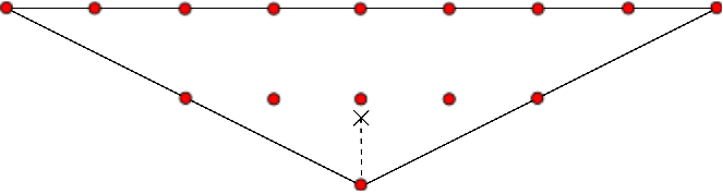
We can already verify mirror symmetry at the level of the Hilbert polynomial:
| (64) |
Figure 7 shows the points of representing the basis of morphisms .
3.3.7. Hamiltonian isotopies
There is an alternative way to express the relationship between and , which is by a Hamiltonian isotopy. There is a Hamiltonian function on such that the time- flow of takes to . During the intermediate times of this isotopy the Lagrangian will not be admissible (or even close to it), but at the end of the isotopy admissibility is restored. This observation is used when we consider wrapped Floer cohomology in section 7.
This isotopy also allows us to identify the intersection points for different values of . For this reason, we will write as simply .
4. A degeneration of holomorphic triangles
Since we have set up our Lagrangians as fibered over paths, a holomorphic triangle with boundary on the Lagrangians composed with the projection is a holomorphic triangle in the base, which is an annulus, with boundary along the corresponding paths. The triangles that are most interesting are those that pass over the critical value (possibly several times). In general, such triangles are immersed in the annulus, and, after passing the the universal cover of the annulus, are embedded. Hence, we can regard such triangles as sections over a triangle in the base of a Lefschetz fibration having as base a strip with a –family of critical values. Once this is done, we can apply a TQFT for counting sections of Lefschetz fibrations developed by Seidel [41, 39].
We consider the deformation of the Lefschetz fibration over the triangle where the critical values bubble out along one of the sides. At the end of this degeneration, we count sections of a trivial fibration over a –gon, along with sections of identical fibrations, each having a disk with one critical value and one boundary marked point. Each of these fibrations is equipped with a Lagrangian boundary condition given by following the degeneration of the original Lagrangian submanifolds. The sections of the trivial fibration over the –gon can be reduced to counts in the fiber, while the counts of the other parts are identical, and can be computed directly using the techniques of [39].
4.1. Triangles as sections
Let and be two degree zero morphisms whose Floer product we wish to compute. Suppose that contributes to this product. Let denote a disk with three boundary punctures, and a complex structure that is allowed to vary. To find the coefficient of in , we count pseudo-holomorphic triangles, that is, pseudo-holomorphic maps that send the punctures to and the boundary components to . Various authors have studied the construction of such invariants; we follow the theory as developed by Seidel in [41, 39].
Because we want to make contact with the theory of pseudo-holomorphic sections of Lefschetz fibrations, we need to import the setup from [39, §2.1]. Let be a exact symplectic Lefschetz fibration. We choose primitive for the symplectic form such that the Liouville vector field defined on the fiber by points outward along the boundary of . The flow of defines a collar , and we let be the function on a neighborhood of given by projection to the factor. We pick an almost complex structure on the base of the fibration, we always consider an almost complex structure on the total space which is compatible relative to , meaning
- (1)
is integrable in a neighborhood of each critical point,
- (2)
is a -holomorphic map,
- (3)
For each fiber , the form is symmetric and positive definite
- (4)
on a neighborhood of the horizontal boundary of , satisfies .
Later on, in Section 4.4, we will also need to consider which are horizontal, meaning that preserves the horizontal subspaces of the symplectic connection. Once we extend the Lagrangian boundary condition Section 4.2 so that our Lagrangians are compact in each fiber, these conditions imply that the curves we wish to count lie in a compact subset disjoint from the horizontal boundary [39, Lemma 2.2]. The second condition is particularly useful because it allows us to study pseudo-holomorphic curves by projecting them to the base of the fibration.
Consider the projection of such a triangle to the base by . This yields a 2-chain on the base with boundary on the corresponding base paths with corners at the points . This projection is not necessarily embedded, so the next step is to pass to the universal cover of the base. Let denote infinite strip which is the universal cover of the annulus, and let denote the induced fibration. We denote by the covering map. When drawing pictures in the base , we can represent it as , with the infinite direction drawn vertically. With this convention, the path lifts to a -family of paths which have slope .
Figure 8 shows the universal cover of , with the base paths for , , and .

The choice of lift of determines a lift of and , which then determines a lift of and of , which in turn determines where the lift of any must lie. By looking at the slopes of the base paths involved, we obtain the following proposition:
Proposition 4.1.
In the terminology of Definition 4, Suppose that lies in the fiber indexed by , and that lies in the fiber indexed by . Then any contributing to the product is for some , that is, it lies in the fiber indexed by
We can rephrase this proposition as saying that we can introduce a second grading on where is generated by for , and that respects this grading.
We must now consider two cases: either the input generators and lie in different fibers of , or they lie in the same fiber. The rest of this section is devoted to case where and lie in different fibers, which is the more difficulty one. In the case where and lie in the same fiber, the preceding proposition says that the output must also lie in the same fiber. This means that we can compute the contribution of to by counting triangles that lie entirely in this fiber, since the projection of such a triangle to the base must be constant. We will employ an alternative strategy where we perturb one of the base paths, say , by a small amount so that there are no points where all three base paths intersect. This forces the triangle in the fiber to spread out over a small triangle in the base, so that in particular it cannot be constant. With this proviso, the arguments in this section apply without exception.
Now we show that any triangles contributing to the product of interest are sections of the Lefschetz fibration :
Proposition 4.2.
Let be a pseudo-holomorphic triangle contributing to the component of in , such that and do not lie in the same fiber of . Then there is a triangle in bounded by appropriate lifts of and , a holomorphic isomorphism , and a pseudo-holomorphic section , such that .
Conversely, any pseudo-holomorphic section with boundary on which maps the corners to contributes to the coefficient of in .
Proof.
Since is a map from a simply-connected domain, there is a lift . Since and are not in the same fiber, the image of cannot be contained entirely within a fiber. The triangle and the lifts of the are determined by the considerations from the previous proposition. Clearly defines a 2-chain in , which by maximum principle is supported on . By positivity of intersection with the fibers of , all components of this 2-chain are positive, and the map is a ramified covering. However, if the degree were greater than one, then would have to wind around more than once, contradicting the boundary conditions we placed on the map .
Since the projection is holomorphic, the composition is a holomorphic map which sends the boundary to the boundary and the punctures to the punctures, so it is a holomorphic isomorphism, and we let be its inverse.
For the converse, uniformization for the disk with three boundary punctures yields a complex structure on and a map , such the composition is the desired triangle in . Composing this with yields the triangle in . ∎
Proposition 4.3.
Suppose lies in the fiber indexed by , and in the fiber indexed by . Then the sections in Proposition 4.2 cover the critical values of the Lefschetz fibration times, where
- •
if and are both non-negative or both non-positive.
- •
if and have different signs.
Proof.
We identify with . The critical values lie at the points .
If and are both non-negative or both non-positive, then the triangle is entirely to one side of the vertical line where all the critical values lie.
Suppose and have opposite signs and . Then the output point lies at , which has the same sign as . The side of corresponding to crosses the line at , while the side corresponding to crosses at , so the distance is , and in fact the set contains points in this interval.
If , the output point at has the same sign as , and so we need to look at where intersects the line . This happens at , and the distance to is . ∎
With the notation introduced so far, we can state the main result of our computation for .
The proof of Proposition 4.4 is where most of the technical work of this paper is spent, and it will occupy Sections 4.2–4.6. Sections 4.2 and 4.3 present a technique for degenerating the total space of the Lefschetz fibration to break these counts into simpler pieces. Sections 4.4 and 4.5 compute these pieces, and Section 4.6 determines the signs.
We shall now reformulate Proposition 4.4 in algebro-geometric terms. Let
| (66) |
be the homogeneous coordinate ring of . We write elements of as degree homogeneous polynomials in the variables . Define
| (67) |
and set, for , ,
| (68) |
Proposition 4.5.
Take and , then in ,
| (69) |
where if and have different signs, and otherwise.
Proof.
The case where and have the same sign is obvious.
Suppose that and , and suppose that . Then we have , and .
| (70) |
Since , we have
| (71) |
| (72) |
and the monomial on the right is just . The other cases are similar. ∎
The operation determines a product, . The sign is present to connect the conventions for an -category at those of a dg-category; in the case all morphisms have degree zero the sign is trivial. The following proposition states how our Lagrangian intersections give rise to a distinguished basis of the homogeneous coordinate ring . From the preceding propositions, we can deduce Theorem 1.1.
Proposition 4.6.
The map defined by
| (73) |
is an isomorphism. We have
| (74) |
Proof.
4.2. Extending the fiber
One problem with our Lagrangian boundary conditions is that they intersect the horizontal boundary . This raises the possibility that as we degenerate the fibration, part of a pseudo-holomorphic section can escape through .
We now describe a technical trick that, by attaching bands to the fiber, allows us to close up the Lagrangians for the purpose of a particular computation, and thereby use only the results in the literature on sections with Lagrangian boundary conditions disjoint from the boundaries of the fibers. Proposition 4.7 states that this attachment does not change the spaces of holomorphic curves that we wish to count, because they do not enter the bands. On the other hand, when we degenerate the fibration, we find that some of these curves degenerate into curves that do enter the bands.
The starting point for this construction is, given inputs and , to consider the portion of the fibration lying over the triangle in the base. We recall the assumption from section 3.2 that the symplectic connection is actually flat near the horizontal boundary. After passing to the universal cover of the base, the symplectic monodromies around the boundaries of can be trivialized, and the fibration is actually symplectically trivial near the horizontal boundary. We also assume that the boundary intersections of our Lagrangians have been positively perturbed as in Section 3.3.4, so that they do not intersect at the boundary. After trivializing the fibration near the horizontal boundary, we find that in each fiber of , there are six points on (three on either component), arising as the symplectic parallel transport of the boundary points of , , and . These are the points where the Lagrangians are allowed to intersect (though is only nonempty if is on the appropriate boundary component of the triangle ). The two sets of three points on each component of are matched according to which Lagrangian they come from, and we extend the fiber to by attaching three bands running between the two components of according to this matching. We call the resulting fibration . We have an embedding .
Over the component of where the Lagrangian boundary condition lies, we extend to , closing it up fiberwise to a circle by letting it run through the corresponding band in . Similarly we close up and to their hat-versions, each passing through a different band.
Figure 9 shows the cylinder with a band attached. The actual extended fiber has three such bands.

It is immediate from the construction that is symplectically a product. Let us use a complex structure which is also a product in this region. Transversality can be achieved using such structures because all intersection points lie in , and hence any pseudo-holomorphic section must also pass through , where we are free to perturb as usual. We have the following proposition:
Proposition 4.7.
Any pseudo-holomorphic section with boundary conditions , lies within .
Proof.
Let denote the projection to the fiber, whose image consist of the bands. Let us consider one band containing the Lagrangian . Introduce coordinates on the band such that the part of the Lagrangian within the band is .
Let be the preimage of the open band under . The set is relatively open. Let . As the map is actually a holomorphic map between Riemann surfaces, the open mapping theorem implies that the image is an open subset of . Also, the boundary of is contained in the union of the Lagrangian (where the boundary of the domain is sent) and the ends of the band (where image of connects to the rest of the holomorphic curve). The only such is the empty set. ∎
4.3. Degenerating the fibration
By propositions 4.2 and 4.7, in order to compute the Floer product between two morphisms and , it is just as good to count sections of the fibration with Lagrangian boundary conditions , , .
In order to obtain these counts, we will consider a degeneration of the Lefschetz fibration. We consider a one-parameter family of Lefschetz fibrations , which for is simply the one we started with. As goes to zero, the fibration deforms so that all of the critical values contained within move toward the side of corresponding to . In the limit, a disc bubble appears around each critical value, and at , the base has broken into a -gon, with “new” vertices along the side corresponding to , each of which joins to a disk with a single critical value. We can equip each fibration with Lagrangian boundary conditions varying continuously with , and degenerating to a collection of Lagrangian boundary conditions for each of the component fibrations at .
The base of the Lefschetz fibration undergoes the degeneration shown in figure 10. This figure shows specifically the case for the product of and . The marked point on the upper portion is the Lefschetz critical value, while the marked points on the lower portion are the Lefschetz critical value and a node.

When performing this construction carefully, it is better to describe this family as a smoothing of the degenerate end. Let be a disk with boundary punctures. We emphasize that the conformal structure of is fixed. Let be a symplectically trivial Lefschetz fibration. Let denote the disks with one boundary puncture that are our “bubbles”. For each let denote a Lefschetz fibration with a single critical value, and which is trivial near the puncture. Let the symplectic monodromy around be denoted .
We will equip each of the components of this fibration with a Lagrangian boundary condition as follows.
- •
The base has one boundary component corresponding to , one boundary component corresponding to , and boundary components corresponding to . Since the fibration is trivial, it suffices to describe each boundary condition in the fiber. Over the point where and come together, we identify the fiber with that of , and take and to be the corresponding Lagrangians.
- •
Over the boundary components of corresponding to , we construct a sequence of Lagrangians. At the puncture where and come together, we take to have the same position relative to (already constructed) that has relative to in the original fibration. As we pass each of the new punctures where the disks are attached, the monodromies must be applied. So we let
(75) This can be done so that, over the puncture where and come together, and intersect as the original and do.
- •
Over the disks , we take a Lagrangian boundary condition which interpolates between and . This is possible because each contains a single Lefschetz critical value.
Note that at this stage we only care about the twists up to Hamiltonian isotopy, but we will make a particular choice in §4.4, as required by the technical considerations there. This gives us such that and have one intersection point over -th new puncture of .
Since the boundary conditions agree over the corresponding punctures, we can glue the components over and with large gluing length in order to obtain for small , which has three boundary components and critical values all near the boundary. There is a family of Lefschetz fibrations interpolating between back to our original , along which the critical values move back to their original points.
We equip and with complex structures, and equip with a family of complex structures converging to those in the limit. All total spaces are equipped with relatively compatible almost complex structures.
Now we appeal to the gluing theorem [39, Proposition 2.2] telling us how the curve counts behave under the degeneration.
Proposition 4.8.
The count of pseudo-holomorphic sections of , with Lagrangian boundary conditions , is obtained from the counts of sections of and by gluing together sections whose values over the punctures match.
Proof.
Considering pseudo-holomorphic sections of the fibrations , as long as the gluing length is large, the sections for will be obtained from sections over and by gluing sections with matching values at the punctures [39, Proposition 2.2]. During the deformation from to , no Floer strip breaking can occur because our Lagrangians , do not bound any strips, even topologically, so the count remains the same at . ∎
4.4. Horizontal sections over a disk with one critical value
We now determine the counts of pseudo-holomorphic sections of the Lefschetz fibrations using the theory of horizontal sections developed by Seidel in [39]. In particular we will apply results from section 2.5 of that paper, so we adopt its notation. This theory involves analysis of the symplectic connection, whose horizontal subspaces are the symplectic orthogonal subspaces to the fibers, and the symplectic parallel transport defined by horizontal lifting of paths in the base of the fibration.
In order for this technique to work, we need to set up carefully a model Lefschetz fibration over a base , the disk with one end, in order to ensure that all the sections we need to count are in fact horizontal. The key properties are:
- •
Transversality of the boundary conditions over the strip-like end. This means that we cannot use a standard model Dehn twist fibration, but need to introduce a perturbation somewhere.
- •
Non-negative curvature. The curvature of the symplectic connection is a two-form on the base with values in functions on the fibers (the Lie algebra of the group of Hamiltonian diffeomorphisms), and we require that this two-form evaluated on a positive basis of the tangent space to the base yields a non-negative function on the fiber. The standard model Dehn twist fibration has non-negative curvature, but requiring the perturbation to have non-negative curvature imposes a constraint.
- •
Vanishing action of horizontal sections. This imposes a further constraint on the perturbation.
As we progress through the construction, the definitions of all of these terms will be recalled.
The first step is to construct a fibration which is flat away from the critical point, following section 3.3 of [39]. Let be the Riemann surface (a negative half-strip which has been rounded off with a half-disk).
Let denote the fiber, which is a cylinder with three bands attached. The vanishing cycle is the equator of the cylinder. The circle running through the core of one of these bands is . Equip with a symplectic form such that is exact. Over , we let be a trivial fibration and equip with 1-form and 2-form which are pulled back from the fiber (to get a symplectic form we add the pullback a positive 2-form , but this does not affect the symplectic connection). Following the pasting procedure described in [39, §3.3] (though with the cut on the right rather than the left), we can complete this fibration to one where the monodromy around the boundary is , a standard model Dehn twist supported near the vanishing cycle. The result has non-negative curvature, is actually trivial on the part of the fiber away from the support of the Dehn twist, and is flat over the part of the base away from the critical value.
For this fibration, there is a Lagrangian boundary condition which over the end corresponds to the pair . Of course, these are not transverse since is identity in the band. Hence we will perturb the symplectic form by a term which depends on a Hamiltonian. We will introduce the perturbation in a neighborhood of the edge . Let be a cutoff function which
- •
is supported in ,
- •
vanishes along the bottom, left and right sides of , and
- •
has .
Figure 11 shows the base of the fibration; the region where has support is shaded.

Let be a Hamiltonian function on the fiber , and let be its vector field defined by . Then over , where our fibration was originally trivial with pulled back from the fiber, consider
| (76) |
| (77) |
This modifies the symplectic connection as follows: Let denote the general vertical vector. Then if , and is its horizontal lift
| (78) |
If we denote by again the horizontal lift with respect to the trivial connection, we have . Since , this means that as we parallel transport in the negative -direction through the region , we pick up a bit of the Hamiltonian flow of , compared with the trivial connection. By adjusting the function , we can ensure that the parallel transport along the boundary in the positive sense picks up , the time 1 flow of .
We must compute the curvature of this connection. This is the 2-form on the base with values in functions on the fibers given by . It will suffice to compute for and , a positive basis. We have and .
| (79) |
The first term vanishes because is horizontal for the trivial connection, the second term because , and the third because . This leaves . By our assumptions on , this is non-negative as long as .
We equip the deformed fibration with a Lagrangian boundary condition given by parallel transport of around the boundary. This picks up a Dehn twist and the time 1 flow of , so over the end we have the pair .
A horizontal section is a map such that . The importance of such sections is that, while they are determined by the symplectic connection, they are pseudo-holomorphic for any horizontal complex structure , meaning an almost complex structure that preserves and for which the projection is holomorphic.
The action of a section is defined to be . The symplectic area of is then . The identity relating action to energy is ([39], eq. 2.31)
| (80) |
for any horizontal complex structure . Here is the splitting induced by the connection, and is the function determined by the curvature as . In our example is supported near the critical point and in , where .
A direct consequence of (80) is the following:
Proposition 4.9.
If the curvature of is non-negative, and if is a -holomorphic section with , then is horizontal and the curvature function vanishes on the image of .
With all this in mind, we choose our Hamiltonian as follows:
- •
and near . This ensures that the fibration is still trivial near the horizontal boundary and that the curvature is non-negative within .
- •
achieves its global maximum of near and on the “cocore” of the band in . It achieves its minimum along the vanishing cycle, and has no other critical points in the cylinder or lying on (which intersects the vanishing cycle and the cocore once). The first condition implies that horizontal sections passing through the cocore do not pick up any curvature, while the second is there in order to ensure that is a transverse pair.
- •
The flow has the property that consists of one point lying on the cocore of the band. At this point, the tangent space to is a small clockwise rotation of the tangent space to .
This implies that this intersection point has degree zero. To see this, recall from Section 3.3.5 that the fiber has foliation by circles. We extend this foliation into the attached bands, foliating each band by intervals. The Dehn twist preserves this foliation, so it admits a grading in the sense of [41, (12i)], namely an -valued lift of the -valued function defined on the Lagrangian Grassmannian bundle. We can choose the lift to be zero in the bands, where is the identity. The Lagrangians and do not rotate with this foliation, so they admit gradings. Thus, if we equip with some grading and with the induced grading, the -valued grading functions for and differ by a small amount. Since tangent space to is a small clockwise rotation of the tangent space to , the intersection point has degree zero.
After this setup, we come to the problem of determining the set of -holomorphic sections satisfying which are asymptotic to over the end.
Proposition 4.10.
Let be a horizontal complex structure. Then consists of precisely one section. It is horizontal, has , and is regular.
Proof.
The first step is to construct a horizontal section. Any horizontal section, if it exists, is determined by parallel transport of the point throughout . Consider the section over given by . This is horizontal outside , since the fibration is trivial over . In , the fact that lies at a critical point of means that is the same as for the trivial connection, so the section is horizontal there as well. Near the singularity, the fibration is trivial in the band where lies, so extends to a horizontal section .
For this section, we compute . Since lies in the region where is trivial, . Since passes through the point where , the contribution vanishes.
Since , any must also have action . To see this, note that is exact on each fiber of the boundary Lagrangian . This implies that , where is a one-form on , and is a function on . Thus
| (81) |
The first term on the right-hand side does not depend on , and the second term, which is the net change in along , depends on the asymptotic data for , which is the same for all .
Because the curvature of is non-negative, proposition 4.9 implies that is horizontal. Since and are both asymptotic to , they are equal. Hence .
It remains to show that is regular. The linearization of parallel transport along trivializes such that the boundary condition is mapped to a family of Lagrangian subspaces which, as we traverse in the positive sense, tilt clockwise by a small amount. That follows from Proposition 11.13 of [41]. On the other hand, Lemma 2.27 of [39] applies to the section , implying . We could also appeal to Lemma 11.5 of [41] (with and ) to see that . Hence as well. ∎
4.5. Polygons with fixed conformal structure
Recall from section 4.3 the trivial fibration , with fiber , where is a a disk with boundary punctures. We have symplectically. We equip with a product almost complex structure , where is the complex structure on .
Proposition 4.11.
The -holomorphic sections are in one-to-one correspondence with -holomorphic maps .
Proof.
Given , write with respect to the product splitting. Since is a product each component is pseudo-holomorphic in the appropriate sense. But is the identity map because is a section. This correspondence is clearly invertible. ∎
This reduces the problem of counting sections to the problem of counting maps . We emphasize that we are counting maps from a Riemann surface with a fixed conformal structure.
The maps are holomorphic maps between Riemann surfaces, and hence their classification is mostly combinatorial. However, because we are in a situation where the conformal structure on the domain is fixed, we are not quite in the situation described, for example, in [41, §13]. The holomorphic curves we are looking for have non-convex corners and hence boundary branch points or “slits,” and if the situation is complicated enough they may also have branch points in the interior. However, the condition that the conformal structure of the domain is fixed makes this an index zero problem, which is to say it prevents these slits and branch points from deforming continuously. The question is then, given a combinatorial type of such a curve, what conformal structures (with multiplicity) can be realized by holomorphic representatives?
The boundary components of are equipped with Lagrangian boundary conditions . Recall that over the ends where disk bubbles are attached we have , where is the monodromy around the -critical point inside the -th disk bubble. In section 4.4, we refined the construction and made a particular choice for this monodromy:
| (82) |
Since all of these symplectomorphisms are isotopic, we will denote them all by for most of this section.
In order to simplify notation, for the rest of this section 4.5 we will drop the hats and superscript zeros and denote by
| (83) |
the Lagrangians in the fiber which give rise to the boundary conditions over the -punctured disk . Though the monodromies are all denoted by , we actually choose the perturbations slightly differently so as to ensure that this collection of Lagrangians is in general position in ; this is necessary for the argument in Lemma 4.20.
Recall that and are the morphisms whose product we wish to compute. We now regard and . Let denote the unique intersection point.
Recall that the possible output points are indexed by .
We can now state the main results of this section.
Proposition 4.12.
If is such that , then there are homotopy classes of maps satisfying the boundary conditions and asymptotic to at the punctures. For outside this range there are no holomorphic maps satisfying these conditions.
Proposition 4.13.
For each feasible homotopy class from Proposition 4.12, and for each complex structure on , there is exactly one holomorphic representative .
The strategy of proof is first to prove Proposition 4.12, which is done in §4.5.1. Then we show the existence of holomorphic representatives for some conformal structure (§4.5.2), and show that the number of representatives does not depend on the conformal structure. By degenerating the domain we are able to show uniqueness (§4.5.3).
4.5.1. Homotopy classes
The analysis of homotopy classes requires some explicit combinatorics, which we shall now set up. Recall that is a cylinder with three bands attached, one for each of . We will classify homotopy classes of maps by their boundary loop , which must be contractible, traverse in order, and hit the intersection points in order. That they arise as the boundary of a holomorphic map controls their behavior within the bands.
Let us use to frame the cylinder, so that winding around the cylinder is computed with respect to . Let be a basepoint which is located in the band near the intersection points . Let denote a loop that enters the cylinder from the bottom, veers right, winds around once, and goes back downward to . We also have a class that is represented by the loop , oriented upward through the cylinder. Note that and generate a free group in .
Lemma 4.14.
winds times relative to . winds times relative to . winds times relative to .
Proof.
We are using the symbols to represent certain Lagrangians in a single fiber , but we can compute the windings by comparing our situation to certain fibers of the original fibration. In the original fibration, and intersect in the fiber containing . Thus we have that winds times relative to . Now winds times relative to by construction. Finally, in the original fibration and intersect in the fiber containing , and the relative winding in that fiber is . In the current context, this becomes the winding of relative to . Thus the winding of relative to in current context is . ∎
The only unknown is how many times the boundary path traverses , , , etc., as we traverse the boundary in the positive sense. The argument from Proposition 4.7 shows that a holomorphic map cannot enter the bands corresponding to and . Hence the portion of our loop along and lies within the cylinder, and therefore it is determined by the choices of , and .
As for the portion of the loop along , this can be represented by a sequence of integers , where represents the number of times we wind around .
With these conventions in place, we can compute the winding of a choice of paths satisfying the boundary and asymptotic conditions. We record the parts of the computation:
- •
Passing from to by a short upward path on contributes
(84) - •
The winding around the cylinder along as we pass from to is
(85) - •
The winding around the cylinder along as we pass from to is
(86) - •
Passing from to by a short downward path on contributes to the winding around the cylinder.
Adding up these contributions and using the fact that , we get a total of . Thus, if we go up on and down on , we pick up the class for the loop from to .
Thus, the class corresponds to the choice for . The homotopy class of any other path can be computed from this as follows:
- •
Taking another path on contributes a factor on the right.
- •
Passing from to along contributes the word
(87) where , and this class is added on the right.
- •
Going down on rather than up contributes the class on the left, which up to conjugation is the same as adding the class on the right.
Thus the class in question is
| (88) |
The key condition is that this class is trivial in . This means in particular that all of the ’s must cancel out. Because and generate a free group we have the following:
Lemma 4.15.
In the word (88), the ’s cancel out if and only if for , the first nonzero is , the last nonzero is , and the nonzero ’s alternate in sign.
Proof.
The first thing to see is that for . This is because contains an isolated , while contains an isolated . Then we can see that the nonzero ’s must alternate sign, since having two consecutive ’s equal to yields , which has an isolated beta, while having two consecutive ’s equal to would yield an isolated .
Since the nonzero ’s in the range alternate in sign, all the ’s coming from the range cancel, except for possibly the first or the last. This implies that as well, since the only thing that can cancel is the first non-identity factor or the last non-identity factor.
Now the from the first non-identity factor can only cancel the from the last non-identity factor if all the ’s as well as ’s in between cancel. This means that
| (89) |
for the appropriate range of : . Since the ’s are in and they alternate in sign, the only solution to this equation is when all . In this case, the first and the last non-identity factors are in fact consecutive, the first has , while the last has . This shows that it is impossible to have from the first factor cancel a from the last factor.
In general, we find that each is canceled by a from the next non-identity factor, so that the nonzero ’s alternate sign for , the first nonzero is , and the last nonzero is . ∎
By passing to , we obtain the relations
| (90) |
| (91) |
Equation (90) is implied by Lemma 4.15, while (91) determines which the homotopy class contributes to.
The sequences which solve the constraints are in one-to-one correspondence with sequences such that . In one direction, we extend the sequence by , and set
| (92) |
In the other direction, given , we can solve for using this equation the initial condition . Since the signs of the nonzero alternate, and the first nonzero term is , we will have , and since the final nonzero term is , we will have , thus inverting the correspondence. This yields solutions.
Plugging this into the summation in (91), we have
| (93) |
because the summation telescopes. This is simply minus the number of ’s in the sequence . Thus we obtain
| (94) |
The right hand side is always an integer between and , and it takes the value for choices of the sequence . Thus homotopy classes of maps exist for such that , and there are such classes. This proves Proposition 4.12.
4.5.2. Existence of holomorphic representatives for some conformal structure
The first step in characterizing the holomorphic representatives of these homotopy classes is to prove the existence of holomorphic sections for some conformal structure. This is also essentially combinatorial.
We begin with some general concepts that will be useful in the proof.
Definition 5.
Let be a piecewise smooth loop. A subloop of is the restriction to a collection of intervals . The indexing set inherits a cyclic order from , and we require that for each , is a self-intersection of . Thus simply “skips” the portion of between and . A subloop is called simple if it is non-self-intersecting.
Note that a subloop is not the same as a loop formed by segments of joining self-intersections. Such an object is only a subloop if the segments appear in a cyclic order compatible with .
Definition 6.
A piecewise smooth loop is said to have the (weak) positive winding property (PWP) if the winding number of around any point in is non-negative. The loop is said to have the strong positive winding property (SPWP) if every subloop has the positive winding property.
Lemma 4.16.
A loop has SPWP if and only if every simple subloop has PWP.
Proof.
The “only if” direction is contained in the definition. Suppose that every simple subloop of has PWP. If is a subloop that is not simple, then by splitting at a self-intersection, we can write as the composition of two proper subloops. Repeating this inductively, we can write as the composition of simple subloops. By hypothesis, each of these subloops winds positively, and the winding of about a point is the sum of the contributions from each of the simple subloops. ∎
The next lemma shows that the strong positive winding property is stable under branched covers. Suppose is a loop and is a point where the winding number of is . Taking the cover branched at , we can lift to a path . The path is a loop that covers .
Lemma 4.17.
Suppose has SPWP. Then has SPWP.
Proof.
Suppose that does not have SPWP. Then some subloop does not have PWP. By Lemma 4.16, we may take to be a simple subloop. Thus winds around some region once clockwise, and we have , where is the chain consisting of this region with coefficient . Pushing and forward under the branched cover, we obtain a subloop , and chain such that . Since is purely negative, no cancellation can occur when we push forward, and is purely negative as well. Thus winds negatively about a point in the support of , which contradicts SPWP for . ∎
Lemma 4.18.
Suppose is a piecewise smooth loop with SPWP. Then there is a map holomorphic on the interior of such that .
Proof.
The idea of the proof is to iteratively take branched covers of the plane and lift so as to reduce the density of winding. So let be a point where the winding number is . Taking the branched cover at , we obtain as in Lemma 4.17 a lift that covers once and has SPWP. Repeating this process and using Lemma 4.17 to guarantee that the lift always has SPWP, eventually we obtain a simple piecewise smooth loop with positive winding. This loop bounds a simply connected region in , where is the Riemann surface resulting from the branched covering construction. By the Riemann mapping theorem, there is a map from this region to the unit disk , biholomorphic on the interior and continuous on the closure, that maps each boundary segment to an arc in and each corner to a point on . Let be the inverse of that map. Composing with the covering yields the desired map . ∎
Fix a choice of homotopy class of polygons , which essentially means fixing a choice for the sequence . Passing to the universal cover of the fiber, fix a choice of lift . Let be any point. Because the boundary loop is contractible in , it lifts to a closed loop in . In fact is contained in a domain which is isomorphic to a domain in , and with this identification, we have the following.
Lemma 4.19.
The boundary loop has SPWP.
Proof.
The key observation is that the slopes of the paths through the cylinder are positive and monotonically decreasing. If we frame the cylinder using , then
- •
has slope
- •
has slope
- •
has slope
- •
has slope .
Only at the intersection between and does the slope increase.
Hence as we traverse , or any subloop thereof, the slope can only increase at one point. This point is either where the subloop either uses or skips over .
Now we use some elementary plane geometry. Suppose that is an oriented polygonal path in the plane (possibly self-intersecting), all of whose sides have positive slope. Suppose that winds negatively around some point . We claim the slope has to increase at no fewer than two vertices. We prove this by induction on the number of sides .
Checking cases proves the claim when and is a triangle. See figure 12(a).
Suppose for induction that the claim is true for . Now we prove the claim if is a simple -gon, so assume for a contradiction that is a simple -gon that winds negatively and has at most one vertex where the slope increases. We assume that , so there must be a side such that at both ends there is a decrease in slope. We remove the side from the -gon and extend the two incident sides and in order to obtain an -gon . Since has at most one vertex where the slope increases, so does : Since the slope decreased at both and at , it will decrease at the new vertex . See Figure 12(b). Since the original simple loop winds negatively, the new loop must also wind negatively around some point. This contradicts the induction hypothesis. Now we have established the claim for simple -gons.

Now suppose is a self-intersecting -gon, that winds negatively around . Using Lemma 4.16, we can find a simple subloop winding negatively around . Since is a simple -gon for some , it must have at least two vertices where the slope increases. For each vertex of where the slope of increases, there is a vertex in the original polygon where the slope increases, either at itself, or at some point in the interval of that was deleted at . Thus, since has at least two vertices where the slope increases, so does .
∎
Having chosen a lift of the boundary loop, define a -chain on whose multiplicity at is the winding number of around . This has .
Lemma 4.20.
There is a complex structure on and a holomorphic map such that .
Proof.
Lemma 4.19 allows us to apply Lemma 4.18, which yields map . More precisely, the complex structure on is the one obtained from uniformization of the region bounded by the simple lift of at the end of the construction in 4.18, as a Riemann surface with boundary and punctures (at the non-smooth points of the loop). ∎
Pushing the map from Lemma 4.20 down to , we obtain the existence of a holomorphic representative in the homotopy class , for a particular complex structure on the domain.
4.5.3. The moduli space of holomorphic representatives with varying conformal structure
Let denote the moduli space of -holomorphic maps in the homotopy class . Let denote the moduli space of such maps with varying conformal structure on the domain. Let denote the moduli space of conformal structures on the disk with boundary punctures. There is a natural map which forgets the map.
Lemma 4.21.
For any , we have and .
Proof.
Let the intersection points be regarded as positive punctures and let be regarded as a negative puncture. Then by the conventions for Maslov index, we have that all of these intersection points have index , for as we go , , …, , and , the Lagrangian tangent space tilts clockwise by a small amount. Then by Proposition 11.13 of [41] (with for the negative puncture), we have .
Furthermore, the operator is a Cauchy–Riemann operator acting on the line bundle , so the results of Section (11d) of [41] apply. The hypotheses of Lemma 11.5 are satisfied with and , so . ∎
Lemma 4.22.
The map is a proper submersion of relative dimension zero (that is, a finite covering).
Proof.
The index is the expected dimension of the space of curves with fixed conformal structure. When we allow the conformal structure to vary, this adds dimensions, so has expected dimension . Lemma 4.21 implies , so is a manifold of dimension .
If is a point where the map is not a submersion, we must have . On the other hand consists of infinitesimal deformations of the map which do not change the conformal structure on the domain, and so is equal to , which is zero by the previous lemma. Hence is a submersion.
The properness of is an instance of Gromov–Floer compactness. The only thing to check is whether, as we vary , any strips can break off. This is impossible because our boundary conditions do not bound any bigons in . ∎
Lemma 4.23.
The map has degree one.
Proof.
For this Lemma we will pass to the Gromov–Floer compactification . Because no bigons can break off, this compactification consists entirely of stable disks, and is also a proper submersion. Hence to count the degree of , it will suffice to count the points in the fiber of over a corner of , which is to say when the domain is a maximally degenerate stable disk.
A maximally degenerate stable disk consists of a trivalent graph without cycles, with infinite edges , and a disk with three boundary punctures for each . The boundary punctures of are labeled by elements of . The elements of correspond to nodes of the stable disk, while the elements of correspond to boundary punctures of the smooth domains in . The homotopy class determines the Lagrangian boundary conditions on each component , and the asymptotic values at the boundary punctures labeled by . The position of the nodes labeled by is not determined a priori.
Looking at the Lagrangians , , …, shows that any three of them bound triangles, and that such triangles are determined by two of the corners. Hence by tree-induction starting at the leaves of stable disk (those for which two punctures are labeled by ), the positions of all the nodes are determined by , or we run into a contradiction because no triangles consistent with the labeling exist.
Furthermore, in each homotopy class of triangles consistent with the labeling of , there is exactly one holomorphic representative.
Hence there is at most one stable map from the stable domain to consistent with the homotopy class .
Thus we have shown that the degree of is either zero or one. On the other hand, Lemma 4.20 shows that is not empty, so the degree must be one. ∎
4.6. Signs
In order to determine the signs appearing in the counts of triangles, we need to specify the brane structures on the Lagrangians . Since fibers over a curve in the base, and its intersection with each fiber is a curve, the tangent bundle of is trivial, and we can define a framing of using the vertical and horizontal tangent vectors at each point. Using this framing, we can give a trivial structure, which is induced by product of the trivial structures on the horizontal an vertical tangent bundles.
Although we have not said much about it up until now, strictly speaking the generators of are not canonically identified with intersection points . Rather, each intersection point gives rise to an abstract -dimensional –vector space, the orientation line . Following [41, Ch. 11], this line is canonically isomorphic up to multiplication by a positive number with the determinant line of a certain Fredholm operator . The moduli space of pseudo-holomorphic curves is canonically oriented relative to these lines.
In the case , where all the intersections have degree , there is a preferred choice of trivialization for . Let . Then we have horizontal-vertical splittings
| (95) |
The intersection point has degree as a morphism from to , and moreover both and tilt clockwise by a small amount as we pass from to .
Let denote the half-plane with a negative puncture. We define the orientation operator , acting on the product bundle , where the boundary condition in the first factor is the short path , while that in the second factor is the short path . By [41, Eq. (11.39)], there is a canonical isomorphism
| (96) |
which for our purposes we take as the definition of . On the other hand, is the direct sum of the operators and , which have vanishing kernel and cokernel. Hence
| (97) |
where all isomorphisms are canonical. This gives us a preferred choice of isomorphism .
Proposition 4.24.
Taking the preferred isomorphisms for all generators for , all of the holomorphic triangles found above have the same sign. Hence, after possibly reversing all off the preferred isomorphisms , all of them have a positive sign.
Proof.
Let be a triangle with positive punctures at and and negative puncture at . Let denote the linearized operator at . Gluing onto the chosen orientation operators and in that order gives another orientation operator for the point , and we want to compare the two orientations for the line .
The linearized operator is an operator in the pulled back tangent bundle . The bundle has a splitting into horizontal and vertical subspaces given by the symplectic connection. Over the boundaries of , the Lagrangian boundary condition also splits. Recall from the discussion on gradings in Section 3.3.5 that we have phase maps on horizontal and vertical subspaces, which measure rotation with respect to the foliations by circles on the base and fiber respectively. These serve to give us preferred trivializations of and . With respect to these trivializations, the Lagrangian boundary conditions move only by a small amount: in the horizontal space, has essentially constant phase, while in the vertical space, moves in such a way that it never crosses the the line corresponding to the circle foliation on the fibers.
The next step is to observe that the boundary conditions for the operator are essentially the same independent of the map and of the chosen degree zero generators , and that hence all of the maps must contribute with the same sign. In all cases we have an operator in a trivial rank two vector bundle, with split Lagrangian boundary conditions, each factor of which is trivial. Additionally, each pair of Lagrangians at a puncture has the same local form, namely they are related by a small clockwise rotation in both the horizontal and vertical directions. The orientation operators used to define the orientation lines are also essentially the same for every point . Hence the relative sign between the determinant of and must be the same for each map .
If the signs are all positive, we are done. Otherwise by reversing our choice of generator for every line we obtain bases for the groups in which all curves contribute positively.
∎
5. A tropical count of triangles
Abouzaid, Gross and Siebert have proposed a definition of a category defined from the tropical geometry of an integral affine manifold, which is meant to describe some part of the Fukaya category of the corresponding symplectic manifold. The starting point for this definition is an integral affine manifold . The objects are then the non-negative integers, with when , and chains on when . The composition is defined by counting a certain type of tropical curve that is balanced after addition of tropical disks.
The motivation is that the non-negative integers correspond to certain Lagrangian sections of a special Lagrangian torus fibration over , such that the intersection points between and lie precisely over the points in . The tropical curves then correspond to the pseudo-holomorphic polygons counted in the A∞ operations.
The Lagrangians considered above are essentially an example of this symplectic setup, so it is encouraging that our computation agrees with the expectation of Abouzaid-Gross-Siebert. The tropical triangles counted in their definition correspond closely to the pseudo-holomorphic triangles found in Section 4.
5.1. Tropical polygons
Let denote the canonical torsion-free flat connection on associated to the affine structure. The following definitions are due to Abouzaid [4].
Definition 7.
Let be a two-dimensional singular affine manifold with focus-focus singularities, and let be a non-singular point. Let be a tree all of whose edges are finite. Label one univalent vertex , and denote the other univalent vertices by . A tropical disk in ending at is a balanced tropical embedding , satisfying the following conditions.
- (1)
,
- (2)
For , is a singular point of the affine structure, and maps the (unique) edge incident to into a monodromy-invariant line of the singularity.
In the case at hand, there is only one singularity, so the only such tropical disks are line segments emanating from the singular point in the monodromy-invariant direction. If there were more singularities with intersecting monodromy-invariant lines, we could obtain more complicated tropical disks.
Definition 8.
Let be points of , with . Let be a metric ribbon tree with infinite edges. One infinite edge, the root, is labeled with and it is the output. The other infinite edges, the leaves, are labeled with in counterclockwise order and these are the inputs. Assign to the region between and the weight , and give the region between and weight . Orient the tree upward from the root, so that each edge has a “left” and a “right” side coming from the ribbon structure. To each edge , assign a weight given by the weight on the left side of minus the weight on the right side of . Define a corrected weight by
| (98) |
Then a tropical polygon modeled on is a map such that:
- (1)
converges on the root edge to and on the -th leaf edge to ;
- (2)
on the edge , the tangent vector to the component satisfies
(99) and converges to on the infinite ends of the root and leaf edges; this differential equation only holds outside a finite set of points where tropical disks are attached;
- (3)
there exists a finite collection of tropical disks such that the union is balanced; the balancing condition at a vertex is the vanishing of the sum of the derivative vectors of the various components of incident at and the integral tangent vectors to at , oriented toward the vertex.
The heuristic motivation for these definitions is that, if we consider a deformation of complex structures in which the torus fibers collapse, we expect that a family of honest holomorphic polygons will likewise collapse onto a piecewise linear complex in . We further expect that two types of local limiting behavior can occur. Some parts of the curve may limit to surfaces that fiber over straight lines in intersecting the torus fibers in paths joining two Lagrangian sections, while other parts may limit to surfaces that fiber over straight lines in intersecting the torus fibers in circles. The latter are what become the tropical disks, while the former become the rest of the tropical polygon. The balancing condition comes from the necessity that these parts can be connected up to form a topological polygon with boundary on the Lagrangian sections. See also [6, Ch. 8].
To unpack this definition, let us restate it in the simplest case, which is that of tropical triangles (this mainly simplifies the issues regarding weights):
Proposition 5.1.
Let and , with and . Let . Let be the ribbon tree with one vertex and three infinite edges. Then a tropical triangle modeled on consists of three maps , , such that
- (1)
is a constant map;
- (2)
;
- (3)
, ;
- (4)
We have and , outside of a finite set of points where tropical disks are attached;
- (5)
there exists a finite collection of tropical disks such that the balancing condition holds.
We can also unpack the equation . The key outcome of the following Lemmas is the insight that the tangent vector increases by times the distance the path travels. Recall that a path is called a geodesic for a connection if .
Lemma 5.2.
Let be a geodesic for . Define by . Then at the point , we have , and .
Proof.
We set . The equation is just the chain rule (note that while ). We have
| (100) |
since is a geodesic. Multiplying this equation by , and using the fact that is tensorial in its subscript, we obtain . ∎
Lemma 5.3.
Let solve . Then if we patch together affine charts along to embed a neighborhood of into , we have
| (101) |
where we use the affine structure of to take differences of points and vectors at different points.
Proof.
Define by , so that is a geodesic. We can embed a neighborhood of into by patching together affine coordinate charts along . Using addition in this embedding, we can write . We have , and
| (102) |
∎
One more thing to note regarding these tangent vectors is how they represent homology classes on the torus fibers of the fibration over .
When considering a tropical curve corresponding to a closed holomorphic curve , each edge of the tropical curve carries an integral tangent vector, which morally represents the class that measures how the holomorphic curve intersects the torus fiber . Because the curve is closed, this class is locally constant along each edge of .
When considering a tropical curve representing a holomorphic curve with boundary on Lagrangian sections , the intersection of with would morally be a path on from to , where is intersection of and . Let be the subset consisting of such cycles, which could also be described as the preimage of under the boundary homomorphism. Hence is a torsor for the kernel of that homomorphism, which is . Using the group structure on , we can identify with the coset
| (103) |
On the other hand, there is an isomorphism . Hence the class of can be regarded as a tangent vector to the base, which is in general real and varies along the tropical curve as and move relative to one another. The tangent vector to the tropical curve is this class.
The balancing condition at a vertex of the tropical polygon amounts to requiring that the three paths , and form a contractible loop. At a point where a tropical disk is attached, the path changes discontinuously by a loop in the homology class in corresponding to the integer tangent vector to the tropical disk.
The last thing to describe for tropical polygons is their multiplicities. There is a multiplicity coming from the different ways to attach a disk to the tropical polygon. If one incoming edge of the polygon has tangent vector corresponding to a path on , and the disk has tangent vector corresponding to a loop on , there are points where the disk can be attached, assuming this determinant is an integer (as it is in the special case below). Otherwise, one must look carefully at exactly where on the torus the paths and are located.
For a tropical disk , we also expect the Gross–Siebert theory to associate a multiplicity . Morally speaking, this number should be a virtual count of holomorphic disks corresponding to , and it should possible to extract this from the “structure” on the affine base in the sense of [22]. In the case at hand, where the base has just a single focus-focus singularity, all of these factors are expect to be one for simple disks, and zero for multiply covered disks [2]. In the rest of this section, we adopt this as an ansatz. Modulo this ansatz, we show in Proposition 5.4 that the tropical curve counts agree with the holomorphic curve counts computed in Section 4. From a certain point of view, this may be regarded as evidence for the ansatz itself, since tropical curve invariants are intentionally designed to correspond to holomorphic curve invariants, and we have computed the latter.
In summary, the multiplicity of a tropical polygon will have both the Gross–Siebert factors counting how many holomorphic disks are in each class, as well as simpler factors counting how many ways these classes of disks can be attached.
Remark 11.
After this paper was originally written, an exposition of the closely related idea of jagged paths appeared [18, Definition 3.2]. In that paper, the various multiplicities are packaged in a different way, but it turns out the that tropical curve counts defined there also agree, in the case of , with the holomorphic curve counts computed in Section 4. The multiplicities we seek are packaged into certain series where runs over certain distinguished rays and lines in . See [18, §3] for more explanation. In our case, there are two such rays emanating from the singularity of the affine structure in the monodromy invariant directions. Our ansatz is equivalent to the fact that the corresponding series reduce, in appropriate choices of coordinates, to and respectively. The salient feature is that these series have a linear term with coefficient and no higher degree terms.
5.2. Tropical triangles for
We now write out explicitly the tropical curves contributing to the triangle products in the case of . Let us use coordinates where the point has coordinates
There is one family of simple tropical disks that emanate from the singularity on the line in the vertical direction. Their primitive tangent vectors are .
Figure 13 shows the the tropical triangle representing the contribution of to the product of and . This triangle has multiplicity . The singularity of the affine structure is placed so as to emphasize the tropical disk ending at the singularity.

Proposition 5.4.
Let and , and take , , and .
Suppose and have different signs, and let , and . If , there is one tropical triangle connecting these three points. It is balanced after the addition of either or tropical disks, depending on the position of the singularity. The multiplicity of this curve is . If does not lie in this range, there is no triangle.
Suppose that and have the same sign. Then unless there is no triangle, and when there is exactly one, which is represented geometrically by the line segment joining and .
Proof.
When and have the same sign the tropical triangle can have no tropical disks attached to it. Therefore the tropical triangle is simply a line segment which passes through the three points, and this only exists if lies on the line between and .
As for when and have different signs, let us consider the case , , , and hence . The other cases are related to this by obvious reflections and re-namings.
By Proposition 5.1, a tropical triangle consists essentially of two maps , together with some copies of the tropical disk and their multiples.
- •
The leg of the tree connecting to cannot have any tropical disks attached, since both endpoints lie on the same side of the line . We can apply Lemma 5.3 to obtain the tangent vector at as times the difference between the endpoints, or
(104) - •
The leg of the tree connecting to crosses the line at some point , where tropical disks can be attached. It may bend there, and continue on to , where the balancing condition must hold. This shows that the portion of connecting to must be parallel to . Hence must be on the line joining and . We obtain the position of :
(105) - •
By Lemma 5.3 at the tangent vector is given by times the difference of the endpoints and :
(106) we use the subscript to denote this is the tangent vector coming from the left.
- •
If the singularity of the affine structure occurs below the point , then tropical disks are line segments going up from the singularity to in the direction . Adding the vector to , we obtain , the tangent vector from the right,
(107) which is parallel to , as it must be. This shows that we must attach a collection of tropical disks whose total weight is .
- •
If the singularity of the affine structure occurs above , then tropical disks are line segments going down from the singularity to in the direction , but there is also the monodromy to be taken into account. First we must act on by the monodromy to get
(108) Adding the vector to this, with , gives the same result as before for . However, in this case we are attaching a collection of disks with total weight .
- •
The leg propagates in the direction from to . As it does so, the tangent vector increases by , which is parallel to . By comparing affine lengths of the segment of from to and the segment of from to , we have the proportion
(109) and
(110) Thus
(111) Verifying the balancing condition at .
Now that we know which tropical curves contribute, we must compute their multiplicities. The tropical curve constructed above uses the tropical disk or times. This means that either we attach a single simple disk times, or we attach some multiple covers of the disk in some fashion as to achieve a total multiplicity of . By our ansatz, only the simple disks contribute, and each with multiplicity one.
Attaching simple disks does introduce a multiplicity, since there are multiple places to attach this disk. In fact, we have , so there are a total of places for disks to be attached. Thus we get the multiplicity or , which are equal and give the desired result.
∎
Remark 12.
The fact that the multiplicities and are equal is an illustration of the general phenomenon that the exact position of the singularity along its invariant line does not matter for tropical curve counts.
6. Parallel monodromy–invariant directions
In this section we describe a class of affine manifolds to which the results obtained for naturally generalize. Consider an integral affine manifold , compact with boundary. We require that has the following properties. Recall that a focus-focus singularity has a monodromy invariant direction, corresponding to the tangent vector field that is fixed by the monodromy.
- (1)
The boundary faces of are straight with respect to the affine structure.
- (2)
The singularities of are focus-focus singularities, and the monodromy–invariant directions of all singularities are parallel.
- (3)
There is an affine linear function such that any corners of occur at extreme values of .
Remark 13.
The condition that the monodromy–invariant directions are parallel is equivalent to the existence of a global integral vector field, or a vector invariant under parallel transport along an arbitrary path in minus the singular points. This vector field spans .
6.1. Symplectic forms
Let denote the singularities of . Let be the image of under , and let . We split up along the monodromy invariant lines of each singularity, and obtain intervals , with fibrations . Choosing an affine function on such that are coordinates, has corresponding complex coordinates , while the coordinate on is .
Each piece is an affine manifold whose horizontal boundary consists of two straight lines (since has no corners but at the extreme values of ), and hence we are in the situation of section 3.1. We obtain a symplectic form for which the symplectic connection of foliates the horizontal boundary facets of .
Corresponding to each focus–focus singularity, we glue in a Lefschetz singularity. The discussion in section 3.2 applies directly. The result is a manifold with a Lefschetz fibration , and such that the horizontal boundary faces of are foliated by the symplectic connection. Let denote the critical values of .
If does not have vertical boundary facets, but rather corners, we simply cut off the corners to introduce horizontal boundary facets. This modification only applies to the symplectic geometry constructions, and the relevant tropical geometry is still that of the original .
We recall that is an annulus . Let denote the fiber over , and the fiber over .
6.2. Lagrangian submanifolds
As before, the construction of Lagrangian sections proceeds by taking paths in the base and a Lagrangian in the fiber, and sweeping out a Lagrangian in the total space by symplectic parallel transport. Potentially, we have more freedom than in the mirror to .
The admissible Lagrangian submanifolds we consider have boundary conditions given by a complex curve in along each boundary face. This gives two complex curves and for the bottom and top horizontal boundary faces. At the vertical boundary faces, we have corresponding complex curves and . These are fibers of the fibration , and to be admissible requires the Lagrangian to end on this fiber. If has a corner rather than a vertical boundary, then the fiber corresponds to a vertical boundary created by cutting off the corner, and the admissibility condition requires the Lagrangians to intersect this fiber in a prescribed real curve.
Thus, a Lagrangian submanifold may be constructed by taking a Lagrangian in , and a path in the base joining to , and taking the parallel transport. If corresponds to a corner, we have only one choice for , and if corresponds to a corner, this imposes a constraint on and . In order to obtain sections of the torus fibration, we choose to be a curve which is a section of the fibration by circles of constant on each fiber, and to be a section of the fibration of the base by circles of constant . Thus when drawing as an annulus, appears as a spiral.
As an example, consider the degree six del Pezzo surface , which may be obtained from by blowing up two points that do not lie on the same ruling line. The moment polytope of is a rectangle. By doing toric blowups at opposite corners, we obtain with a toric boundary divisor consisting of six -curves, and the moment polytope is a hexagon. Alternatively, by doing almost toric blowups [43] on opposite sides of the hexagon, we obtain with an anticanonical divisor of four components with self-intersections . The base affine manifold has four sides and two singularities with parallel monodromy invariant directions.
Passing over to the mirror side, we consider Lagrangians in the symplectic manifold . Then we can choose independently
- (1)
the number of times the initial Lagrangian winds around the fiber ,
- (2)
the number of times winds around the base between the and the first singularity,
- (3)
the number of times winds around the base between the two singularities, and
- (4)
the number of times winds around the base between the second singularity and .
This gives rise to a -parameter family of Lagrangians. Under mirror symmetry, all of them correspond to line bundles. We expect that is a mirror to the degree del Pezzo surface with a -component anticanonical divisor. The parameters correspond to .
Though we can construct many Lagrangians this way, in order to compute Floer cohomology and identify the basis with , we must choose a family of Lagrangians corresponding to the tensor powers of an ample line bundle. First we choose as a reference path in the base, over which lies , a Lagrangian satisfying the boundary conditions. We take to be a certain path in the base: the number of times that must wind between the singularities and the vertical boundaries/corners is determined by : it is essential that the number of turns makes between two consecutive singularities (or between a boundary and the neighboring singularity) is the affine width of the corresponding portion of . An equivalent condition is that the winds at unit speed. If has a vertical boundary face rather than a corner, the intersection of with the fiber at that boundary must be a curve that, relative to , makes a number of turns equal to the affine length of the corresponding vertical boundary face. Then we choose to be a path in the base whose slope is times the slope of , relative to . We also make sure that in the fiber, the slope is times the slope of (relative to in each fiber).
6.3. Holomorphic and tropical triangles
Having chosen a family of Lagrangians corresponding to the powers of an ample line bundle, we find that after positively perturbation, is concentrated in degree when . The techniques of section 4 allow us to compute the holomorphic triangles contributing to the multiplication
| (112) |
Looking at the winding numbers of the Lagrangians in the base once again yields an auxiliary -grading. For fixed values of this -grading on the input, one can determine the number of times that triangles contributing to the product cover the critical values ; call these numbers . Then the degeneration process breaks the triangle into copies of the fibration over a disk with single critical value, as well a trivial fibration over a -gon. Over the disks the count of sections is , while the analysis of sections over the -gon still goes through because, in the fiber, the Lagrangian boundary condition is still a sequence of curves on the cylinder whose slope changes monotonically. Hence the matrix coefficients of this product are binomial coefficients of the form .
In this degeneration argument, the Lefschetz singularities that come from different focus-focus singularities are not distinguished, while in the case of tropical triangles, different singularities of the affine structure contribute differently to the tropical curves. We find that this family of triangles, with total count , corresponds to several tropical triangles with , indexed by ordered partitions of , with allowed as a part (of which there are ). The triangle uses the tropical disk emanating from the -th singularity either or times, and the multiplicity of is . The equality of the total counts
| (113) |
follows from comparing the coefficients of in the equation
| (114) |
7. Mirrors to divisor complements
In this section we examine the relationship between the wrapped Floer cohomology of our Lagrangians and the cohomology of coherent sheaves on complements of components of the anticanonical divisor in . Let denote the anticanonical divisor which is the union of a conic and a line . We can consider the divisor complements , , and . The torus fibration can be restricted to such a complement, and T-duality gives the same space as before, but with a different superpotential, reflecting the counts of holomorphic disks intersecting the remaining components of the anticanonical divisor.
| Variety | Anticanonical divisor | Mirror space | Superpotential |
|---|---|---|---|
Once again, the cohomology of coherent sheaves corresponds to Floer cohomology of the Lagrangian submanifolds .
Removing a divisor from a compact variety changes the cohomology of a coherent sheaf , since, for example, sections of with poles along are regular on the complement , so that is not finitely generated in general.
On the symplectic side, changing the superpotential by dropping a term modifies the boundary condition for our Lagrangian submanifolds . Some parts of that were required to lie on the fiber of are no longer so constrained, and it is appropriate to wrap these parts of . The algebraic structure associated to is then wrapped Floer cohomology , which is the limit , where is an appropriate Hamiltonian function (a more precise definition is given below). The limit will not be finitely generated in general, since it potentially contains trajectories of joining to of any length. The general theory of wrapped Floer cohomology is developed in [5].
7.1. Algebraic motivation
In order to motivate the symplectic constructions of wrapped Floer cohomology, it is useful to understand the algebraic side first. The starting point is the following proposition ([40], statement (1.10)).
Proposition 7.1.
Let be a smooth quasiprojective variety over , a hypersurface, and the complement. Write , where is the canonical section of the line bundle . Let be a coherent sheaf on . Multiplication by defines an inductive system
| (115) |
and the limit is
| (116) |
We spell out the application of this proposition to each of the cases we consider
- •
: Since is a line, we identify and take . Thus
(117) where the limit is formed with respect to multiplication by . An element of is a rational function , where is a homogeneous polynomial of degree .
- •
: Since is a conic, we identify and take . Thus
(118) where the limit is formed with respect to multiplication by . An element of is a rational function , where is a homogeneous polynomial of degree .
- •
: Since is a cubic, we identify and take . Thus
(119) where the limit is formed with respect to multiplication by . An element of is a rational function , where is a homogeneous polynomial of degree .
For the purposes of computation, a useful simplification comes from noting that the line bundles may become isomorphic over the complements.
- •
: Since , all the line bundles are isomorphic over it.
- •
: The complement of a smooth conic in has , generated by . The defining section is an isomorphism over , and so as well.
- •
: Since , all the line bundles are isomorphic over it as well.
7.2. Wrapping
In this subsection we describe the geometric setup for wrapped Floer cohomology in the mirrors of , and .
7.2.1. Completions
Wrapped Floer cohomology is formulated in terms of noncompact manifolds containing noncompact Lagrangian submanifolds. These can be defined as (partial) completions of compact manifolds with boundary.
The starting point for all three cases is the original Lefschetz fibration containing the Lagrangians . We define completions , , and . This process involves replacing a boundary component with an infinite end, either on the base or in the fiber of the Lefschetz fibration.
- •
: The manifold retains a boundary component at the top horizontal boundary, corresponding to the fiber of the superpotential . The fibers of are completed at the other, bottom, end. The base annulus is completed to a cylinder , and the fibration is extended over this cylinder.
- •
: The manifold retains a boundary component at the bottom horizontal boundary, corresponding to the fiber of the superpotential . The fibers are completed at the other, top, end. The base annulus is completed to a cylinder , and the fibration is extended over this cylinder.
- •
: The manifold has no boundary, and the fibers are completed at both ends. The base annulus is completed to a cylinder , and the fibration is extended over this cylinder.
The torus fibration on extends to these completions, and yields torus fibrations over completed bases ,, .
- •
is a half-plane with singular affine structure given by removing the bottom boundary from and extending in that direction.
- •
is a half-plane with singular affine structure given by removing the top boundary from and extending in that direction.
- •
is an entire plane with singular affine structure given by removing all boundaries from and extending in all directions.
The Lagrangian submanifolds are extended to ; In all cases, we extend into whatever ends are attached so as to be invariant under the Liouville flow within the end. However, in the case of , respectively , we still have the boundary condition that is required to end on (the complex hypersurface contained in the top boundary), respectively (contained in the bottom boundary).
7.2.2. Hamiltonians
The most crucial difference between the three cases comes from the choices of Hamiltonians that are be used to perform the wrapping. The Hamiltonians we consider are the sum of contributions from the base and the fiber.
Let be the pullback of a function on the base cylinder which is a function of the radial coordinate only. Writing the symplectic form on the base as , where is a function of , we take to be a convex function of on the compact part , and linear in on the ends. We also require , with minimum on the central circle . Since vanishes on the fibers, is horizontal.
The fiber Hamiltonian is chosen differently in each case. The main constraint is that its differential must vanish at any boundary component which may still be present. The construction is most convenient if we assume the completion preserves the -symmetry that rotates the fibers. If denotes the moment map for this action, we can take to be a function of . Since is tangent to the fibers, we have
| (120) |
which allows us to compute the flow of term by term.
We use the same base Hamiltonian for all cases. The specific choice of in each case is as follows.
- •
: Let be a function with a minimum at the top of the fiber, convex in on the compact part, and linear in on the bottom end.
- •
: Let be a function with a minimum at the bottom of the fiber, convex in on the compact part, and linear in on the top end.
- •
: Let be a function with a minimum in the two-thirds of the way down from the top of the compact part of the fiber, convex in on the compact part, and linear in on the ends.
In each case, the total Hamiltonian achieves its minimum along a torus in , which is one of the fibers of the torus fibration over . Since is a section of the torus fibration, has a unique minimum on , and hence there is a unique constant chord for , which corresponds to the identity element . The cases are:
- •
: The minimum is along the torus corresponding to the midpoint of the top edge of , where the generator lies. All of the Lagrangians for intersect this torus at the same point. As an intersection point of and , the minimum corresponds to for .
- •
: The minimum is along the torus corresponding to the midpoint of the bottom edge of , where the generator lies. All of the Lagrangians for intersect this torus at the same point. As an intersection point of and , the minimum corresponds to for .
- •
: The minimum is along the torus two-thirds of the way from the top of the middle fiber of the map , where the generator lies. All of the Lagrangians for intersect this torus in the same point. As an intersection point of and , the minimum corresponds to for .
Remark 14.
The Hamiltonians we obtain as are not admissible in the usual sense, because they vanish at some boundaries, and, even in the case , are not linear with respect to a cylindrical end. Closer to our situations are the Lefschetz admissible Hamiltonians considered by Mark McLean [34], that are precisely those functions on the total space of a Lefschetz fibration that are the sum of admissible Hamiltonians on the base and fiber separately.
7.2.3. Generators
Given Lagrangian submanifolds of , equipped with Hamiltonian , and , we get Floer cohomology complexes generated by time- trajectories of starting on and ending on . As usual the differential counts inhomogeneous pseudo-holomorphic strips. We also have continuation maps
| (121) |
given by counting strips where the inhomogeneous term interpolates between and . At the homology level, the continuation maps form an inductive system, and we define the wrapped Floer cohomology
| (122) |
Our purpose in this section is simply to set up an enumeration of the generators of in each of the three cases. These generators can also be regarded as intersection points . In order to make the situation as convenient as possible for our later arguments, we refine our choice of Hamiltonians so as to ensure that is actually for some ; thus we can identify wrapped Floer cohomology generators with intersection points of our original Lagrangians. This is done by adjusting the slopes of our Hamiltonians on the ends.
- •
We take the base Hamiltonian so that the time– flow completes turn on the cylindrical ends of the base.
- •
For cases and , we take the fiber Hamiltonian so that the time– flow completes turn on the cylindrical end of the fiber.
- •
For case , we take the fiber Hamiltonian so that the time– flow completes turn at the top of the fiber, and turn at the bottom of the fiber.
In all cases the total Hamiltonian we use is .
The way to understand the flow of is to first apply , then . The flow of wraps in the fiber, while the flow of , when it completes a loop in the base, performs the monodromy of the Lefschetz fibration around that loop, which undoes some of the wrapping due to .
We can relate to as follows:
- •
: we have .
- •
: we have . Note that the same cannot be said with in place of ; in that case the two Lagrangians intersect the bottom boundary (where no wrapping occurs) in different points.
- •
: we have . Again the same cannot be said with in place of .
In order to identify generators with intersection points, we perturb the boundary intersection points in a positive sense just as before. In the cases with boundary, where the Hamiltonian is supposed to have a minimum at the boundary, it is useful to perform this perturbation in an extra collar attached to the boundary, so that the Lagrangians still intersect at the minimum of if they did prior to the perturbation. Once this is done, we can identify
| (123) |
where in case , in case , and in case . This identification is compatible with the gradings, which shows that for , the Floer complex is concentrated in degree zero, and so has vanishing differential. Recall that the generators of the last group are identified with .
Once we are in the range , we find that as increases, new generators are created, none are destroyed, and the generators that already exist are “compressed” toward the minimum of . This gives rise to naive inclusion maps for , where . In terms of fractional integral points, this corresponds to the map which is dilation by the appropriate factor centered at the point corresponding to the minimum of .
We can index the points of with two indices. The index corresponds to the column lying at , while the index that indexes points within a column, and which lies in in the compact case, is now unbounded in the positive direction in case , in the negative direction in case , and in both directions in case . We use the notation for these points.
7.3. Continuation maps and products
We saw above that for , the generators of all have degree , so there are no differentials, and we can identify these complexes with their homologies. In order to obtain the wrapped Floer cohomology, we must determine the continuation maps.
Let it be understood that we require in case , in case , and in case .
To get started, we consider the wrapped Floer cohomology of with itself. Each complex has a distinguished element , sitting at the minimum of . The complexes are filtered by action, and the continuation maps are non-increasing with respect to this filtration. Under the continuation map, ; and are the unique generators of minimal action in their respective complexes, and in fact their actions are equal, so the only strip is the constant map to the minimum.
At this point we bring in the product structure.
Proposition 7.2.
Let one of the Lagrangians for . Under the identification
| (124) |
The product
| (125) |
which counts inhomogeneous pseudo-holomorphic triangles corresponds to the product
| (126) |
counting pseudo-holomorphic triangles with no inhomogeneous term.
Proof.
First we recall the equation for the product in the wrapped setting. The disk with three boundary punctures is equipped with strip-like ends: at the inputs they are parametrized by , while at the output we have . is also equipped with a closed one form , whose restriction to vanishes, such that on the strip-like ends of , has the form , and for the two inputs and the output respectively. The curves we count are solutions of
| (127) |
Because is closed and has no first homology, we may find a primitive such that , and we assume on the boundary corresponding to . Denoting by the flow of for time , we can define a new map , meaning that for , we take and flow it for time by . This has the effect of collapsing each Hamiltonian chord to a single point. Then the map is pseudo-holomorphic without inhomogeneous term, but with a domain-dependent almost complex structure obtained by conjugating the original by at each point.
We must relate the products
| (128) |
defined with respect to this domain-dependent almost complex structure to the operation that we studied in Section 4, where the complex structure was fixed. We fix attention to one strip-like end, say the one corresponding to and . On this end the complex structure depends only on . There is a continuation map
| (129) |
counting strips with a domain-dependent almost complex structure that interpolates between and . We claim that, in our situation, all such strips are constant. This means that the bases of intersection points on the two sides of the continuation map correspond. These continuation maps intertwine the product with respect to and the one defined using , implying that these products agree when expressed in the basis of intersection points on either side of the correspondence.
It remains to prove the claim that all the continuation strips are constant. Let denotes such a strip. Because the Hamiltonian flow preserves the structure of the Lefschetz fibration, each for is a complex structure with the property that the tangent space to a fiber is complex, and the projection to the base is holomorphic, once we equip the base with a suitable complex structure . As is pseudo-holomorphic with respect to , this implies that has the property that its differential at each point has rank either or . Thus the image of is a set whose boundary is contained in the images of the Lagrangians and . Because there are no topological strips in the base joining different intersection points of the base paths, we conclude that must be constant, and the image of is contained in a fiber. But in the fiber there are also no topological strips joining different intersection points. Hence itself is constant. ∎
When the differentials on the Floer complexes vanish, the identification of the products holds at the chain level as well. Tracing the isomorphisms through, we find that the product with induces the naive inclusion map on generators
| (130) |
Due to the compatibility of the product with the continuation maps, and the fact that under continuation, we find that the naive inclusion maps commute with the continuation maps:
| (131) |
Thus the continuation map agrees with the naive inclusion map, at least on those generators which are in the image of . It follows that the continuation maps agree with the naive inclusion maps, at least for large enough depending on a particular generator. Hence
| (132) |
where the limit is formed with respect to the continuation maps, or with respect to the naive inclusion maps, or (what is equal) the multiplications by the various elements .
Spelling this out a bit more gives a precise correspondence with section 7.1. Consider the isomorphism
| (133) |
- •
: For , this isomorphism identifies with .
- •
: For , this isomorphism identifies with .
- •
: For , this isomorphism identifies with .
Thus the directed systems computing wrapped Floer cohomology are identified with those computing the cohomology of line bundles on the divisor complements.
We can identify the basis of with , where is the completion of the affine manifold. The sets embed in and this latter is their limit as ; the map is dilation by centered at the minimum of .
Using the products we computed in section 4, we can identify this basis for with a basis of , and complete the proof of Theorem 1.2
- •
: The point of corresponds to the function for , and for . In this case can be arbitrarily large, so the exponent of is allowed to be negative.
- •
: The point of corresponds to the function for , and for . In this case can be negative, so the exponent of is allowed to be negative, while the exponent of is non-negative.
- •
: The point of corresponds to the function for , and for . In this case , so the exponents of and are allowed to be negative.
References
- [1] Mohammed Abouzaid, Homogeneous coordinate rings and mirror symmetry for toric varieties, Geom. Topol. 10 (2006), 1097–1157 (electronic). MR 2240909 (2007h:14052)
- [2] Mohammed Abouzaid, 2009, Private communication.
- [3] Mohammed Abouzaid, Morse homology, tropical geometry, and homological mirror symmetry for toric varieties, Selecta Math. (N.S.) 15 (2009), no. 2, 189–270. MR 2529936
- [4] by same author, Toward a tropical Fukaya category, Talk given in the MSRI workshop “Tropical Structures in Geometry and Physics”, December 2009, video available on MSRI website.
- [5] Mohammed Abouzaid and Paul Seidel, An open string analogue of Viterbo functoriality, Geom. Topol. 14 (2010), no. 2, 627–718. MR 2602848
- [6] Paul S. Aspinwall, Tom Bridgeland, Alastair Craw, Michael R. Douglas, Mark Gross, Anton Kapustin, Gregory W. Moore, Graeme Segal, Balázs Szendrői, and P. M. H. Wilson, Dirichlet branes and mirror symmetry, Clay Mathematics Monographs, vol. 4, American Mathematical Society, Providence, RI, 2009. MR 2567952 (2011e:53148)
- [7] Denis Auroux, Mirror symmetry and -duality in the complement of an anticanonical divisor, J. Gökova Geom. Topol. GGT 1 (2007), 51–91. MR 2386535 (2009f:53141)
- [8] Denis Auroux, Ludmil Katzarkov, and Dmitri Orlov, Mirror symmetry for del Pezzo surfaces: vanishing cycles and coherent sheaves, Invent. Math. 166 (2006), no. 3, 537–582. MR 2257391 (2007g:14045)
- [9] by same author, Mirror symmetry for weighted projective planes and their noncommutative deformations, Ann. of Math. (2) 167 (2008), no. 3, 867–943. MR 2415388 (2009f:53142)
- [10] Philip Candelas, Xenia C. de la Ossa, Paul S. Green, and Linda Parkes, A pair of Calabi-Yau manifolds as an exactly soluble superconformal theory, Nuclear Phys. B 359 (1991), no. 1, 21–74. MR 1115626 (93b:32029)
- [11] Bohan Fang, Chiu-Chu Melissa Liu, David Treumann, and Eric Zaslow, T-duality and homological mirror symmetry for toric varieties, Adv. Math. 229 (2012), no. 3, 1875–1911. MR 2871160 (2012m:14075)
- [12] Sergey Fomin and Andrei Zelevinsky, Cluster algebras. I. Foundations, J. Amer. Math. Soc. 15 (2002), no. 2, 497–529 (electronic). MR 1887642 (2003f:16050)
- [13] Kenji Fukaya, Yong-Geun Oh, Hiroshi Ohta, and Kaoru Ono, Lagrangian intersection floer theory: Anomaly and obstruction, chapter 10, (2007), preprint.
- [14] by same author, Lagrangian Floer theory on compact toric manifolds. I, Duke Math. J. 151 (2010), no. 1, 23–174. MR 2573826 (2011d:53220)
- [15] Alexander B. Givental, Equivariant Gromov-Witten invariants, Internat. Math. Res. Notices (1996), no. 13, 613–663. MR 1408320 (97e:14015)
- [16] Mark Gross, The Strominger-Yau-Zaslow conjecture: from torus fibrations to degenerations, Algebraic geometry—Seattle 2005. Part 1, Proc. Sympos. Pure Math., vol. 80, Amer. Math. Soc., Providence, RI, 2009, pp. 149–192. MR 2483935 (2010b:14080)
- [17] Mark Gross, Paul Hacking, and Sean Keel, Mirror symmetry for log Calabi–Yau surfaces I, preprint: arXiv:1106.4977.
- [18] Mark Gross and Bernd Siebert, Theta functions and mirror symmetry, Written for the JDG2011 conference, arXiv:1204.1991.
- [19] by same author, Affine manifolds, log structures, and mirror symmetry, Turkish J. Math. 27 (2003), no. 1, 33–60. MR 1975331 (2004g:14041)
- [20] by same author, Mirror symmetry via logarithmic degeneration data. I, J. Differential Geom. 72 (2006), no. 2, 169–338. MR 2213573 (2007b:14087)
- [21] by same author, Mirror symmetry via logarithmic degeneration data, II, J. Algebraic Geom. 19 (2010), no. 4, 679–780. MR 2669728 (2011m:14066)
- [22] by same author, From real affine geometry to complex geometry, Ann. of Math. (2) 174 (2011), no. 3, 1301–1428. MR 2846484
- [23] Nigel J. Hitchin, The moduli space of special Lagrangian submanifolds, Ann. Scuola Norm. Sup. Pisa Cl. Sci. (4) 25 (1997), no. 3-4, 503–515 (1998), Dedicated to Ennio De Giorgi. MR 1655530 (2000c:32075)
- [24] Kentaro Hori, Amer Iqbal, and Cumrum Vafa, D-branes and mirror symmetry, preprint: arXiv:hep-th/0005247.
- [25] Kentaro Hori and Cumrun Vafa, Mirror symmetry, preprint: arXiv:hep-th/0002222.
- [26] Ilia Itenberg, Grigory Mikhalkin, and Eugenii Shustin, Tropical algebraic geometry, second ed., Oberwolfach Seminars, vol. 35, Birkhäuser Verlag, Basel, 2009. MR 2508011 (2010d:14086)
- [27] Anton Kapustin, Ludmil Katzarkov, Dmitri Orlov, and Mirroslav Yotov, Homological mirror symmetry for manifolds of general type, Cent. Eur. J. Math. 7 (2009), no. 4, 571–605. MR 2563433 (2010j:53184)
- [28] Maxim Kontsevich, Homological algebra of mirror symmetry, Proceedings of the International Congress of Mathematicians, Vol. 1, 2 (Zürich, 1994) (Basel), Birkhäuser, 1995, pp. 120–139. MR 1403918 (97f:32040)
- [29] by same author, Lectures at ENS, Paris, (Spring 1998), notes taken by J. Bellaiche, J.-F. Dat, I. Marin, G. Racinet and H. Randriambololona.
- [30] Maxim Kontsevich and Yan Soibelman, Homological mirror symmetry and torus fibrations, Symplectic geometry and mirror symmetry (Seoul, 2000), World Sci. Publ., River Edge, NJ, 2001, pp. 203–263. MR 1882331 (2003c:32025)
- [31] by same author, Affine structures and non-Archimedean analytic spaces, The unity of mathematics, Progr. Math., vol. 244, Birkhäuser Boston, Boston, MA, 2006, pp. 321–385. MR 2181810 (2006j:14054)
- [32] N. C. Leung, S.-T. Yau, and E. Zaslow, From special Lagrangian to Hermitian-Yang-Mills via Fourier-Mukai transform, Winter School on Mirror Symmetry, Vector Bundles and Lagrangian Submanifolds (Cambridge, MA, 1999), AMS/IP Stud. Adv. Math., vol. 23, Amer. Math. Soc., Providence, RI, 2001, pp. 209–225. MR 1876070 (2002k:53102)
- [33] Bong H. Lian, Kefeng Liu, and Shing-Tung Yau, Mirror principle. I, Asian J. Math. 1 (1997), no. 4, 729–763. MR 1621573 (99e:14062)
- [34] Mark McLean, Lefschetz fibrations and symplectic homology, Geom. Topol. 13 (2009), no. 4, 1877–1944. MR 2497314 (2011d:53224)
- [35] Robert C. McLean, Deformations of calibrated submanifolds, Comm. Anal. Geom. 6 (1998), no. 4, 705–747. MR 1664890 (99j:53083)
- [36] Alexander Polishchuk and Eric Zaslow, Categorical mirror symmetry: the elliptic curve, Adv. Theor. Math. Phys. 2 (1998), no. 2, 443–470. MR 1633036 (99j:14034)
- [37] Paul Seidel, More about vanishing cycles and mutation, Symplectic geometry and mirror symmetry (Seoul, 2000), World Sci. Publ., River Edge, NJ, 2001, pp. 429–465. MR 1882336 (2003c:53125)
- [38] by same author, Vanishing cycles and mutation, European Congress of Mathematics, Vol. II (Barcelona, 2000), Progr. Math., vol. 202, Birkhäuser, Basel, 2001, pp. 65–85. MR 1905352 (2003i:53128)
- [39] by same author, A long exact sequence for symplectic Floer cohomology, Topology 42 (2003), no. 5, 1003–1063. MR 1978046 (2004d:53105)
- [40] by same author, -subalgebras and natural transformations, Homology, Homotopy Appl. 10 (2008), no. 2, 83–114. MR 2426130 (2010k:53154)
- [41] by same author, Fukaya categories and Picard-Lefschetz theory, Zurich Lectures in Advanced Mathematics, European Mathematical Society (EMS), Zürich, 2008. MR 2441780 (2009f:53143)
- [42] Andrew Strominger, Shing-Tung Yau, and Eric Zaslow, Mirror symmetry is -duality, Nuclear Phys. B 479 (1996), no. 1-2, 243–259. MR 1429831 (97j:32022)
- [43] Margaret Symington, Four dimensions from two in symplectic topology, Topology and geometry of manifolds (Athens, GA, 2001), Proc. Sympos. Pure Math., vol. 71, Amer. Math. Soc., Providence, RI, 2003, pp. 153–208. MR 2024634 (2005b:53142)