跳到论文正文
W Papers独立论文阅读器 arXiv:1109.3061 论文正文 计算阅读时间 · 0%
引用这篇论文根据当前论文元数据生成,正式投稿前建议核对。


License: arXiv.org perpetual non-exclusive license
arXiv:1109.3061v1 [math.NA] 14 Sep 2011

∎

Approximation of weak adjoints by reverse automatic differentiation of BDF methods

Dörte Beigel    Mario S. Mommer    Leonard Wirsching    Hans Georg Bock E-mail: doerte.beigel@iwr.uni-heidelberg.de E-mail: {mario.mommer, leonard.wirsching, bock}@iwr.uni-heidelberg.de Affiliation: Interdisciplinary Center for Scientific Computing (IWR), Heidelberg University. Im Neuenheimer Feld 368, 69120 Heidelberg, Germany. Fax: +49-6221-54 5444.
, Tel.: +49-6221-54 8896 (corresponding).
.
September 13, 2011
Abstract

With this contribution, we shed light on the relation between the discrete adjoints of multistep backward differentiation formula (BDF) methods and the solution of the adjoint differential equation. To this end, we develop a functional-analytic framework based on a constrained variational problem and introduce the notion of weak adjoint solutions. We devise a finite element Petrov-Galerkin interpretation of the BDF method together with its discrete adjoint scheme obtained by reverse internal numerical differentiation. We show how the finite element approximation of the weak adjoint is computed by the discrete adjoint scheme and prove its asymptotic convergence in the space of normalized functions of bounded variation. We also obtain asymptotic convergence of the discrete adjoints to the classical adjoints on the inner time interval. Finally, we give numerical results for non-adaptive and fully adaptive BDF schemes. The presented framework opens the way to carry over the existing theory on global error estimation techniques from finite element methods to BDF methods.

Keywords: 
BDF methods discrete adjoints Petrov-Galerkin discretization
MSC
65L06 65L60 49K40 65L20

1 Introduction

Consider a nonlinear initial value problem (IVP) in ordinary differential equations (ODE) with sufficiently smooth right hand side 𝒇:[ts,tf]×ℝd→ℝd{\bm{f}}:[{t_{\mathrm{s}}},{t_{\mathrm{f}}}]\times\mathbb{R}^{d}\rightarrow\mathbb{R}^{d}

𝒚˙​(t)\displaystyle\dot{{\bm{y}}}(t) =𝒇⁡(t,𝒚⁡(t)),t∈(ts,tf]\displaystyle={\bm{f}}(t,{\bm{y}}(t)),\quad t\in({t_{\mathrm{s}}},{t_{\mathrm{f}}}] (1a)
𝒚⁡(ts)\displaystyle{\bm{y}}({t_{\mathrm{s}}}) =𝒚s.\displaystyle={\bm{y}}_{\text{s}}. (1b)

Consider also a differentiable criterion of interest JJ depending on the final state 𝒚⁡(tf){\bm{y}}({t_{\mathrm{f}}}) of the solution of (1). This is relevant whenever one is not interested in the whole solution trajectory 𝒚⁡(t){\bm{y}}(t) or even the final state 𝒚⁡(tf){\bm{y}}({t_{\mathrm{f}}}), but only in a functional output of these quantities. Note that by standard reformulations (cf. (14, p.93), (7, p.25)) this setting also captures the cases of a parameter-dependent right hand side 𝒇⁡(t,𝒚,𝒑){\bm{f}}(t,{\bm{y}},{\bm{p}}) and a criterion of interest of Bolza type J⁡(𝒚)=∫tstfJ1​(𝒚⁡(t),𝒑)​𝑑t+J2​(𝒚⁡(tf))J({\bm{y}})=\int_{t_{\mathrm{s}}}^{t_{\mathrm{f}}}J_{1}({\bm{y}}(t),{\bm{p}})\mathrm{d}t+J_{2}({\bm{y}}({t_{\mathrm{f}}})).

The adjoint differential equation corresponding to the evaluation of J⁡(𝒚⁡(tf))J({\bm{y}}({t_{\mathrm{f}}})) in the solution of (1) is (see Section 2)

𝝀˙​(t)\displaystyle\dot{{\bm{\lambda}}}(t) =−𝒇𝒚⊺​(t,𝒚⁡(t))​𝝀​(t),t∈(tf,ts]\displaystyle=-{\bm{f}}^{\intercal}_{{\bm{y}}}(t,{\bm{y}}(t)){\bm{\lambda}}(t),\quad t\in({t_{\mathrm{f}}},{t_{\mathrm{s}}}] (2a)
𝝀⁡(tf)\displaystyle{\bm{\lambda}}({t_{\mathrm{f}}}) =J′​(𝒚⁡(tf))⊺.\displaystyle=J^{\prime}({\bm{y}}({t_{\mathrm{f}}}))^{\intercal}. (2b)

The adjoint solution describes the dependency of J⁡(𝒚⁡(tf))J({\bm{y}}({t_{\mathrm{f}}})) on disturbances of the nominal solution 𝒚⁡(t){\bm{y}}(t). Therefore, it is of great importance in the solution of optimal control problems. For example, in indirect approaches based on the Pontryagin minimum principle, (2) appears as part of the optimality conditions.

For an approximation of the solution of (1), the solution of the adjoint differential equation (2) can be computed in two different ways, the continuous adjoint approach or the discrete adjoint approach. The former solves the adjoint differential equation by numerical integration, see for example [12]. Whereas the latter applies automatic differentiation techniques to the numerical integration scheme. This approach, firstly presented in [8], is known as internal numerical differentiation (IND). It has significant advantages in direct derivative-based approaches for the solution of optimal control problems that use integrators, e.g. direct single and multiple shooting.

In the case of Runge-Kutta methods, the discrete adjoint scheme generated by adjoint IND is itself a Runge-Kutta scheme for the adjoint differential equation (2), and thus gives a convergent approximation to the adjoint solution [8, 25]. In the case of continuous and discontinuous Galerkin methods applied to (1), the discrete adjoint scheme yields an approximation to the solution of (2) (see e.g. [19]). The discrete adjoints of discontinuous Galerkin methods for compressible Navier-Stokes equations are, for example, considered in [15].

The situation becomes significantly more complex in the case of multistep methods, as the discrete adjoint schemes of linear multistep methods (LMM) are generally not consistent with the adjoint differential equation (2). But they still provide approximations of the sensitivities J′​(𝒚⁡(tf))​∂𝒚⁡(tf)∂𝒚sJ^{\prime}({\bm{y}}({t_{\mathrm{f}}}))\frac{\partial{\bm{y}}({t_{\mathrm{f}}})}{\partial{\bm{y}}_{\mathrm{s}}} at the initial time ts{t_{\mathrm{s}}} that converge with the rate of the nominal LMM [9, 23]. Due to this property, the multistep BDF method and its discrete adjoint scheme are used successfully in direct methods for the solution of optimal control problems, e.g. in direct multiple shooting [10, 3].

In this contribution, we focus on the relation between the discrete adjoints of variable-order variable-stepsize BDF methods and the adjoints defined by (2). To this end, we construct a suitable constrained variational problem (CVP) in a Banach space setting using the duality pairing between the space of continuous functions and its dual, the space of normalized functions of bounded variation. It turns out that the adjoint of a stationary point of this CVP is the normalized integral of the solution of the Hilbert space adjoint differential equation (2). Motivated by PDE nomenclature, we will call it a weak solution of (2) or shortly weak adjoint. We apply Petrov-Galerkin techniques, and show that with the appropriate choice of basis functions the infinite-dimensional optimality conditions of the CVP are approximated by the BDF method and its discrete adjoint scheme obtained by adjoint internal numerical differentiation of the nominal BDF scheme. In particular, we obtain that discretization and optimization commute in this Banach space setting. Finally, we prove that the finite element approximation of the weak adjoint, which can be computed by a simple post-processing of the discrete adjoints, converges to the weak adjoint on the entire time interval. This result is based on the linear convergence of the discrete adjoints to the solution of (2) on the inner time interval which is shown as well.

This paper is organized as follows. In Section 2 we derive the adjoint differential equation as part of the optimality conditions of an infinite-dimensional constrained variational problem in Hilbert spaces. The BDF method and its discrete adjoint scheme generated by internal numerical differentiation techniques are then described in Section 3. In Section 4 we present the optimality conditions of the constrained variational problem embedded into the Banach space of all continuously differentiable functions. After showing the well-posedness of the optimality conditions and their relation to the Hilbert space optimality conditions, we extend the setting to capture the space of all functions that are continuous and piecewise continuously differentiable. For the Petrov-Galerkin discretization of Section 5 we choose suitable finite element spaces that yield equivalence between the discretized optimality conditions and the BDF scheme together with its discrete adjoint scheme. In Section 6 we start by proving the convergence of the discrete adjoints to the solution of the Hilbert space adjoint equation on the inner time interval. Using this result, we show the convergence of the finite element approximation to the weak adjoint solution. Section 7 presents numerical results on a nonlinear test case with analytic solutions.

2 Initial value problems and their adjoints in a Hilbert space setting

In this section, we derive the adjoint differential equation in a Hilbert space functional-analytic setting. Our goal is to specify the assumptions on the initial value problem, to settle some notation, and to lay the groundwork for the constructions that follow. In particular, we make explicit the connection between the adjoint differential equation and the Lagrange multiplier of the solution of a constrained variational problem in a Hilbert space setting based on the Sobolev spaces usually found in finite element formulations.

2.1 Existence, uniqueness and differentiability of the nominal solution

Assume that the right hand side 𝒇⁡(t,𝒚){\bm{f}}(t,{\bm{y}}) of (1) is continuous on an open set 𝒟⊂ℝ×ℝd\mathcal{{D}}\subset\mathbb{R}\times\mathbb{R}^{d} with (ts,𝒚s)∈𝒟({t_{\mathrm{s}}},{\bm{y}}_{\mathrm{s}})\in\mathcal{{D}} and its first-order partial derivative 𝒇𝒚​(t,𝒚){\bm{f}}_{{\bm{y}}}(t,{\bm{y}}) is continuous on 𝒟\mathcal{{D}}. Thus, according to the Picard-Lindelöf Theorem [14], problem (1) is well-posed in the sense of Hadamard, i.e. it admits a unique solution depending continuously on the input data. Beyond that, the solution 𝒚⁡(t){\bm{y}}(t) is continuously differentiable on an open interval ℐ\mathcal{{I}}, see [14], and we assume that tf{t_{\mathrm{f}}} is chosen such that [ts,tf]⊂ℐ[{t_{\mathrm{s}}},{t_{\mathrm{f}}}]\subset\mathcal{{I}}. Thus, the solution 𝒚⁡(t){\bm{y}}(t) of (1) lies in the Banach space C1​[ts,tf]dC^{1}[{t_{\mathrm{s}}},{t_{\mathrm{f}}}]^{d} of all continuously differentiable functions from [ts,tf][{t_{\mathrm{s}}},{t_{\mathrm{f}}}] to ℝd\mathbb{R}^{d} equipped with the usual norm. Furthermore, the solution 𝒚⁡(t)=𝒚⁡(t,ts,𝒚s){\bm{y}}(t)={\bm{y}}(t;{t_{\mathrm{s}}},{\bm{y}}_{\mathrm{s}}) is continuously differentiable with respect to 𝒚s{\bm{y}}_{\mathrm{s}} and the derivatives 𝒘i​(t)=∂𝒚⁡(t,ts,𝒚s)/∂(𝒚s)i{\bm{w}}_{i}(t)=\partial{\bm{y}}(t;{t_{\mathrm{s}}},{\bm{y}}_{\mathrm{s}})/\partial({\bm{y}}_{\mathrm{s}})_{i} solve [14]

𝒘˙i​(t)\displaystyle\dot{{\bm{w}}}_{i}(t) =𝒇𝒚​(t,𝒚⁡(t))​𝒘i​(t),t∈(ts,tf]\displaystyle={\bm{f}}_{{\bm{y}}}(t,{\bm{y}}(t)){\bm{w}}_{i}(t),\quad t\in({t_{\mathrm{s}}},{t_{\mathrm{f}}}] (3a)
𝒘i​(ts)\displaystyle{\bm{w}}_{i}({t_{\mathrm{s}}}) =𝒆i\displaystyle={\bm{e}}_{i} (3b)

where 𝒆i{\bm{e}}_{i} is the iith unit vector, i∈{1,…,d}i\in\{1,\dots,d\}. Moreover, 𝒘i​(t){\bm{w}}_{i}(t) exists uniquely and is continuously differentiable on [ts,tf][{t_{\mathrm{s}}},{t_{\mathrm{f}}}] since the partial derivative of the right hand side of (3) with respect to 𝒘i{\bm{w}}_{i} is continuous in (t,𝒘i)(t,{\bm{w}}_{i}). The residual of (1a)

𝝆⁡(𝒚):=𝒚˙​(⋅)−𝒇⁡(⋅,𝒚⁡(⋅))\displaystyle{\bm{\rho}}({\bm{y}}):=\dot{{\bm{y}}}(\cdot)-{\bm{f}}(\cdot,{\bm{y}}(\cdot)) (4)

lies in the Banach space C0​[ts,tf]dC^{0}[{t_{\mathrm{s}}},{t_{\mathrm{f}}}]^{d} of all continuous functions from [ts,tf][{t_{\mathrm{s}}},{t_{\mathrm{f}}}] to ℝd\mathbb{R}^{d} equipped with the standard norm ||𝒈||C0​[ts,tf]d=∑i=1d||gi||C0​[ts,tf]\left|\left|{\bm{g}}\right|\right|_{C^{0}[{t_{\mathrm{s}}},{t_{\mathrm{f}}}]^{d}}=\sum_{i=1}^{d}\left|\left|g_{i}\right|\right|_{C^{0}[{t_{\mathrm{s}}},{t_{\mathrm{f}}}]} where ||gi||C0​[ts,tf]=maxt∈[ts,tf]⁡|gi​(t)|\left|\left|g_{i}\right|\right|_{C^{0}[{t_{\mathrm{s}}},{t_{\mathrm{f}}}]}=\max_{t\in[{t_{\mathrm{s}}},{t_{\mathrm{f}}}]}\,\left|g_{i}(t)\right|.

2.2 Lagrange multipliers and adjoint differential equations

The core of this section is the identification of the adjoint as the Lagrange multiplier of a constrained optimization problem in a functional-analytic setting. The ideas described here are of course not new. However, the setting for the case of ordinary differential equations is fundamental for this contribution. Since we have not found it in the literature, we include here a detailed derivation.

Recall that functions in C0​[ts,tf]dC^{0}[{t_{\mathrm{s}}},{t_{\mathrm{f}}}]^{d}, restricted to the open interval (ts,tf)({t_{\mathrm{s}}},{t_{\mathrm{f}}}), form a dense subset of the space L2​(ts,tf)dL^{2}({t_{\mathrm{s}}},{t_{\mathrm{f}}})^{d} of all quadratically Lebesgue-integrable functions. Similarly, recall that the subset C1​[ts,tf]dC^{1}[{t_{\mathrm{s}}},{t_{\mathrm{f}}}]^{d} is dense in the Sobolev space H1​(ts,tf)dH^{1}({t_{\mathrm{s}}},{t_{\mathrm{f}}})^{d} of all L2​(ts,tf)dL^{2}({t_{\mathrm{s}}},{t_{\mathrm{f}}})^{d}-functions with weak derivative in L2​(ts,tf)dL^{2}({t_{\mathrm{s}}},{t_{\mathrm{f}}})^{d} (see (2, Ch.3)). Furthermore, both spaces L2​(ts,tf)dL^{2}({t_{\mathrm{s}}},{t_{\mathrm{f}}})^{d} and H1​(ts,tf)dH^{1}({t_{\mathrm{s}}},{t_{\mathrm{f}}})^{d} are Hilbert spaces.

Knowing this, we embed the initial value problem (1) into an optimization framework and derive the adjoint differential equation as part of the first-order necessary optimality conditions. To this end, we consider the constrained variational problem

min𝒚\displaystyle\min_{{\bm{y}}}\kern 5.0pt J⁡(𝒚⁡(tf))\displaystyle J({\bm{y}}({t_{\mathrm{f}}})) (5a)
s.t.\displaystyle\operatorname{s.t.}\kern 5.0pt 𝒚˙​(t)=𝒇⁡(t,𝒚⁡(t)),t∈(ts,tf]\displaystyle\dot{{\bm{y}}}(t)={\bm{f}}(t,{\bm{y}}(t)),\quad t\in({t_{\mathrm{s}}},{t_{\mathrm{f}}}] (5b)
𝒚⁡(ts)=𝒚s\displaystyle{\bm{y}}({t_{\mathrm{s}}})={\bm{y}}_{\text{s}} (5c)

which is equivalent to evaluating J⁡(𝒚⁡(tf))J({\bm{y}}({t_{\mathrm{f}}})) in the solution of (1). Considering (5) on the space H1​(ts,tf)dH^{1}({t_{\mathrm{s}}},{t_{\mathrm{f}}})^{d}, the Hilbert space Lagrangian ℒ:H1​(ts,tf)d×L2​(ts,tf)d→ℝ\mathcal{L}:H^{1}({t_{\mathrm{s}}},{t_{\mathrm{f}}})^{d}\times L^{2}({t_{\mathrm{s}}},{t_{\mathrm{f}}})^{d}\rightarrow\mathbb{R} of (5) using the L2L^{2}-scalar product is

ℒ⁡(𝒚,𝝀):=J⁡(𝒚⁡(tf))−∫tstf𝝀⊺​(t)​[𝒚˙​(t)−𝒇⁡(t,𝒚⁡(t))]​𝑑t−𝝀⊺​(ts)​[𝒚⁡(ts)−𝒚s]\displaystyle\mathcal{L}({\bm{y}},{\bm{\lambda}}):=J({\bm{y}}({t_{\mathrm{f}}}))-\int_{t_{\mathrm{s}}}^{t_{\mathrm{f}}}{\bm{\lambda}}^{\intercal}(t)\left[\dot{{\bm{y}}}(t)-{\bm{f}}(t,{\bm{y}}(t))\right]\mathrm{d}t-{\bm{\lambda}}^{\intercal}({t_{\mathrm{s}}})\left[{\bm{y}}({t_{\mathrm{s}}})-{\bm{y}}_{\mathrm{s}}\right]

where 𝝀{\bm{\lambda}} is the Lagrange multiplier. The optimality condition of (5) is based on the Fréchet derivative of ℒ\mathcal{L} at (𝒚,𝝀)({\bm{y}},{\bm{\lambda}}) in direction (𝒘,𝝌)({\bm{w}},{\bm{\chi}}) which exists due to Fréchet differentiability of JJ and (17, Ch.0§0.2.5)

ℒ′\displaystyle\mathcal{L}^{\prime} (𝒚,𝝀)​(𝒘,𝝌)=ℒ𝒚​(𝒚,𝝀)​(𝒘)+ℒ𝝀​(𝒚,𝝀)​(𝝌)\displaystyle({\bm{y}},{\bm{\lambda}})({\bm{w}},{\bm{\chi}})=\mathcal{L}_{{\bm{y}}}({\bm{y}},{\bm{\lambda}})({\bm{w}})+\mathcal{L}_{{\bm{\lambda}}}({\bm{y}},{\bm{\lambda}})({\bm{\chi}})
=\displaystyle= {J′​(𝒚⁡(tf))​𝒘​(tf)−∫tstf𝝀⊺​(t)​[𝒘˙​(t)−𝒇𝒚​(t,𝒚⁡(t))​𝒘​(t)]​𝑑t−𝝀⊺​(ts)​𝒘​(ts)}\displaystyle\left\{\displaystyle J^{\prime}({\bm{y}}({t_{\mathrm{f}}})){\bm{w}}({t_{\mathrm{f}}})-\int_{t_{\mathrm{s}}}^{t_{\mathrm{f}}}{\bm{\lambda}}^{\intercal}(t)\left[\dot{{\bm{w}}}(t)-{\bm{f}}_{{\bm{y}}}(t,{\bm{y}}(t)){\bm{w}}(t)\right]\mathrm{d}t-{\bm{\lambda}}^{\intercal}({t_{\mathrm{s}}}){\bm{w}}({t_{\mathrm{s}}})\right\}
+{−∫tstf𝝌⊺(t)[𝒚˙(t)−𝒇(t,𝒚(t))]dt−𝝌⊺(ts)[𝒚(ts)−𝒚s]}.\displaystyle+\left\{\displaystyle-\int_{t_{\mathrm{s}}}^{t_{\mathrm{f}}}{\bm{\chi}}^{\intercal}(t)\left[\dot{{\bm{y}}}(t)-{\bm{f}}(t,{\bm{y}}(t))\right]\mathrm{d}t-{\bm{\chi}}^{\intercal}({t_{\mathrm{s}}})\left[{\bm{y}}({t_{\mathrm{s}}})-{\bm{y}}_{\mathrm{s}}\right]\right\}.

The necessary condition for a stationary point (𝒚,𝝀)∈H1​(ts,tf)d×L2​(ts,tf)d({\bm{y}},{\bm{\lambda}})\in H^{1}({t_{\mathrm{s}}},{t_{\mathrm{f}}})^{d}\times L^{2}({t_{\mathrm{s}}},{t_{\mathrm{f}}})^{d} of (5) is that ℒ′​(𝒚,𝝀)​(𝒘,𝝌)=0\mathcal{L}^{\prime}({\bm{y}},{\bm{\lambda}})({\bm{w}},{\bm{\chi}})=0 holds for all directions (𝒘,𝝌)∈H1​(ts,tf)d×L2​(ts,tf)d({\bm{w}},{\bm{\chi}})\in H^{1}({t_{\mathrm{s}}},{t_{\mathrm{f}}})^{d}\times L^{2}({t_{\mathrm{s}}},{t_{\mathrm{f}}})^{d}. Choosing 𝒘=𝟎∈H1​(ts,tf)d{\bm{w}}={\bm{0}}\in H^{1}({t_{\mathrm{s}}},{t_{\mathrm{f}}})^{d} and only varying 𝝌∈L2​(ts,tf)d{\bm{\chi}}\in L^{2}({t_{\mathrm{s}}},{t_{\mathrm{f}}})^{d} the necessary condition reads

∫tstf𝝌⊺​(t)​[𝒚˙​(t)−𝒇⁡(t,𝒚⁡(t))]​𝑑t+𝝌⊺​(ts)​[𝒚⁡(ts)−𝒚s]=0,∀𝝌\displaystyle\int_{t_{\mathrm{s}}}^{t_{\mathrm{f}}}{\bm{\chi}}^{\intercal}(t)\left[\dot{{\bm{y}}}(t)-{\bm{f}}(t,{\bm{y}}(t))\right]\mathrm{d}t+{\bm{\chi}}^{\intercal}({t_{\mathrm{s}}})\left[{\bm{y}}({t_{\mathrm{s}}})-{\bm{y}}_{\mathrm{s}}\right]=0,\;\forall{\bm{\chi}} (6)

which possesses the same unique solution 𝒚∈C1​[ts,tf]d{\bm{y}}\in C^{1}[{t_{\mathrm{s}}},{t_{\mathrm{f}}}]^{d} as (1). Taking now 𝝌=𝟎∈L2​(ts,tf)d{\bm{\chi}}={\bm{0}}\in L^{2}({t_{\mathrm{s}}},{t_{\mathrm{f}}})^{d} and only varying 𝒘∈H1​(ts,tf)d{\bm{w}}\in H^{1}({t_{\mathrm{s}}},{t_{\mathrm{f}}})^{d} one obtains using integration by parts

[J′​(𝒚⁡(tf))−𝝀⊺​(tf)]​𝒘​(tf)−∫tfts[𝝀˙​(t)+𝒇𝒚⊺​(t,𝒚⁡(t))​𝝀​(t)]⊺​𝒘​(t)​𝑑t=0,∀𝒘\displaystyle\left[J^{\prime}({\bm{y}}({t_{\mathrm{f}}}))-{\bm{\lambda}}^{\intercal}({t_{\mathrm{f}}})\right]{\bm{w}}({t_{\mathrm{f}}})-\int^{t_{\mathrm{s}}}_{t_{\mathrm{f}}}\left[\dot{{\bm{\lambda}}}(t)+{\bm{f}}^{\intercal}_{{\bm{y}}}(t,{\bm{y}}(t)){\bm{\lambda}}(t)\right]^{\intercal}{\bm{w}}(t)\mathrm{d}t=0,\;\forall{\bm{w}}

which possesses the same solution as (2). Under the assumptions of Section 2.1, the unique solution 𝝀⁡(t){\bm{\lambda}}(t) of (2) is continuously differentiable on [ts,tf][{t_{\mathrm{s}}},{t_{\mathrm{f}}}] and depends continuously on J′​(𝒚⁡(tf))⊺J^{\prime}({\bm{y}}({t_{\mathrm{f}}}))^{\intercal}.

3 Efficient solution of initial value problems and sensitivity generation

We now review the numerical solution of ODEs using BDF methods, and the corresponding sensitivity generation using automatic differentiation techniques. We briefly introduce BDF methods with an emphasis on the trajectories they define as functions of time. Then, we show how to obtain discrete adjoints in the BDF context, and review what is known so far about their relation to the solution of (2).

3.1 Backward differentiation formula method

This section follows the lines of (24, p.181ff and p.253f). Consider the backward differentiation formula method

𝒚0\displaystyle{\bm{y}}_{0} =𝒚s\displaystyle={\bm{y}}_{\mathrm{s}} (7a)
∑i=0knαi(n)​𝒚n+1−i\displaystyle\sum_{i=0}^{k_{n}}\alpha_{i}^{(n)}{\bm{y}}_{n+1-i} =hn𝒇(tn+1,𝒚n+1),n=0,…,N−1\displaystyle=h_{n}{\bm{f}}(t_{n+1},{\bm{y}}_{n+1}),\quad n=0,\dots,N-1 (7b)

with a self-starting procedure that begins with k0=1k_{0}=1 (implicit Euler) and increases successively the order of the steps until the maximum order is reached. Note that BDF methods are used up to order 6, since for higher order they become unstable. In practical implementations both the stepsize hnh_{n} and the order knk_{n} are chosen adaptively to obtain better performance. The numerical solution is computed at discrete time points ts=t0<t1<⋯<tN=tf{t_{\mathrm{s}}}=t_{0}<t_{1}<\dots<t_{N}={t_{\mathrm{f}}} with tn+1=tn+hnt_{n+1}=t_{n}+h_{n} and 𝒚n{\bm{y}}_{n} denotes the numerical approximation to the value 𝒚⁡(tn){\bm{y}}(t_{n}). The coefficients αi(n)\alpha_{i}^{(n)} are determined by

αi(n)=hnL˙i(n)(tn+1), where Li(n)(t)=∏j=0,j≠iknt−tn+1−jtn+1−i−tn+1−j\displaystyle\alpha_{i}^{(n)}=h_{n}\dot{L}_{i}^{(n)}(t_{n+1}),\text{ where }L_{i}^{(n)}(t)=\prod_{j=0,j\neq i}^{k_{n}}\frac{t-t_{n+1-j}}{t_{n+1-i}-t_{n+1-j}} (8)

are the fundamental Lagrangian polynomials. Thus, the coefficients depend on the discrete time points and the order. In each step, the BDF method provides a polynomial approximation to the solution 𝒚⁡(t){\bm{y}}(t) of (1) in a natural way through the interpolation polynomial

𝒚⁡(t)|t∈[tn,tn+1]≈∑i=0knLi(n)​(t)​𝒚n+1−i,\displaystyle{\bm{y}}(t)\big|_{t\in[t_{n},t_{n+1}]}\approx\sum_{i=0}^{k_{n}}L_{i}^{(n)}(t)\;{\bm{y}}_{n+1-i}, (9)

also known as dense output. The composition of all these polynomials gives a continuous and piecewise continuously differentiable approximation to the solution 𝒚⁡(t){\bm{y}}(t) on the whole time interval [ts,tf][{t_{\mathrm{s}}},{t_{\mathrm{f}}}].

3.2 Adjoint differentiation of BDF integration schemes

The basic idea of internal numerical differentiation [8] is to differentiate the discretization scheme used to obtain the nominal approximations 𝒚0,𝒚1,…,𝒚N{\bm{y}}_{0},{\bm{y}}_{1},\dots,{\bm{y}}_{N} for specified adaptive components hnh_{n} and knk_{n} using automatic differentiation (AD) techniques either in forward or in adjoint mode. Adjoint IND was first described in [9] for Runge-Kutta integration schemes and later on in [11] for BDF methods. Applying adjoint IND to the BDF scheme (7) we obtain the discrete adjoint scheme

α0(N−1)​𝝀N−J′​(𝒚N)⊺\displaystyle\alpha_{0}^{(N-1)}{\bm{\lambda}}_{N}-J^{\prime}({\bm{y}}_{N})^{\intercal} =hN−1​𝒇𝒚⊺​(tN,𝒚N)​𝝀N\displaystyle=h_{N-1}{\bm{f}}^{\intercal}_{{\bm{y}}}(t_{N},{\bm{y}}_{N}){\bm{\lambda}}_{N} (10a)
∑0≤i≤N−1−ni≤kmaxαi(n+i)​𝝀n+1+i\displaystyle\sum_{0\leq i\leq N-1-n\atop i\leq k_{\max}}\alpha_{i}^{(n+i)}{\bm{\lambda}}_{n+1+i} =hn𝒇𝒚⊺(tn+1,𝒚n+1)𝝀n+1,n=N−2,…,0\displaystyle=h_{n}{\bm{f}}^{\intercal}_{{\bm{y}}}(t_{n+1},{\bm{y}}_{n+1}){\bm{\lambda}}_{n+1},\;n=N-2,\dots,0 (10b)

with input direction J′​(𝒚N)⊺J^{\prime}({\bm{y}}_{N})^{\intercal} and the convention αi(n)=0\alpha_{i}^{(n)}=0 for i>kni>k_{n}, kmax=maxn⁡{kn}k_{\max}=\max_{n}\{k_{n}\} (see also [23]). This scheme forms together with (7) the optimality conditions of the nonlinear program (NLP)

min𝒚\displaystyle\min_{{\bm{y}}}\kern 5.0pt J⁡(𝒚N)​s.t.⁡ (7)\displaystyle J({\bm{y}}_{N})\kern 5.0pt\operatorname{s.t.}\kern 5.0pt\text{ \eqref{eq:BDF}} (11)

with 𝒚⊺:=[𝒚0⊺𝒚1⊺⋯𝒚N⊺]{\bm{y}}^{\intercal}:=\left[\begin{array}[]{cccc}{\bm{y}}^{\intercal}_{0}&{\bm{y}}^{\intercal}_{1}&\cdots&{\bm{y}}^{\intercal}_{N}\end{array}\right]. This NLP is a discretization of the constrained variational problem (5).

The discrete adjoints given by (10) are the exact derivatives of the nominal integration scheme (7) (beside round-off errors). Furthermore, for a BDF scheme with constant order kk, the discrete adjoint 𝝀1{\bm{\lambda}}_{1} converges with the same order kk to the value 𝝀⁡(ts){\bm{\lambda}}({t_{\mathrm{s}}}) of the adjoint solution of (2), cf. [9, 23].
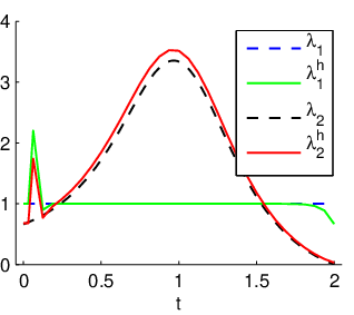
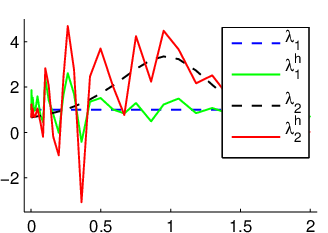
The discrete adjoints are generally inconsistent approximations to the solution of (2) around a nominal approximation passing through {𝒚n}n=0N\{{\bm{y}}_{n}\}_{n=0}^{N}, see Figure 1(b). In the case of constant order kk and constant stepsizes hh, the discrete adjoints coming from the adjoint initialization and adjoint termination are inconsistent as well, whereas the main part, i.e. formula (10b) with n=N−k,…,kn=N-k,\dots,k, gives consistent approximations of order kk, see Figure 1(a).

Refer to caption
(a) Non-adaptive BDF method with constant order and constant stepsizes.
Refer to caption
(b) Adaptive BDF method with variable order and variable stepsize.
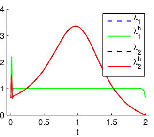
Figure 1: Comparison of discrete adjoints 𝝀h=[λ1h,λ2h]⊺{\bm{\lambda}}^{h}=[\lambda_{1}^{h},\lambda_{2}^{h}]^{\intercal} and analytic solution 𝝀=[λ1,λ2]⊺{\bm{\lambda}}=[\lambda_{1},\lambda_{2}]^{\intercal} of the Hilbert space adjoint differential equation on the Catenary test case (see Section 7).

Due to the inconsistency of the discrete adjoint scheme (10) with the adjoint differential equation (2) discretization and optimization of (5) do not commute in the commonly used Hilbert space setting. This gives rise to the question for a new functional-analytic setting that is suitable for multistep methods. The next sections are devoted to the development of this setting.

4 Solution of the constrained variational problem in a Banach space setting

As seen in the previous section, the Hilbert space setting of Section 2 is not suitable to analyze multistep methods and their discrete adjoints. Here, we propose to embed the constrained variational problem (5) into a Banach space setting and show the well-posedness of the corresponding infinite-dimensional optimality conditions.

4.1 General considerations

Duality pairing

According to Section 2.1, the residual 𝝆⁡(𝒚){\bm{\rho}}({\bm{y}}) of (1a) is an element of the space C0​[ts,tf]dC^{0}[{t_{\mathrm{s}}},{t_{\mathrm{f}}}]^{d}. Thus, we focus on the duality pairing between the Banach space C0​[ts,tf]dC^{0}[{t_{\mathrm{s}}},{t_{\mathrm{f}}}]^{d} and its dual. The Riesz Representation Theorem (21, Ch.5§5.5) states that for every continuous linear functional 𝔏\mathfrak{L} on C0​[ts,tf]C^{0}[{t_{\mathrm{s}}},{t_{\mathrm{f}}}] exists a unique Ψ∈NBV[ts,tf]\Psi\in\NBV[{t_{\mathrm{s}}},{t_{\mathrm{f}}}] such that

𝔏⁡[g]=⟨Ψ,g⟩NBV[ts,tf],C0​[ts,tf]=∫tstfg⁡(t)​𝑑Ψ​(t),\displaystyle\mathfrak{L}[g]=\left\langle\Psi,g\right\rangle_{\NBV[{t_{\mathrm{s}}},{t_{\mathrm{f}}}],C^{0}[{t_{\mathrm{s}}},{t_{\mathrm{f}}}]}=\int_{t_{\mathrm{s}}}^{t_{\mathrm{f}}}g(t)\mathrm{d}\Psi(t), (12)

where the integral is the Riemann-Stieltjes integral (22, Ch.VIII§6). The Banach space NBV[ts,tf]\NBV[{t_{\mathrm{s}}},{t_{\mathrm{f}}}] consists of all normalized functions of bounded variation on [ts,tf][{t_{\mathrm{s}}},{t_{\mathrm{f}}}] that are zero in ts{t_{\mathrm{s}}} and continuous from the right on (ts,tf)({t_{\mathrm{s}}},{t_{\mathrm{f}}}). It is equipped with the total variation norm

||Ψ||NBV[ts,tf]=sup∑i=1m|Ψ⁡(ti)−Ψ⁡(ti−1)|\displaystyle\left|\left|\Psi\right|\right|_{\NBV[{t_{\mathrm{s}}},{t_{\mathrm{f}}}]}=\sup\sum_{i=1}^{m}\left|\Psi(t_{i})-\Psi(t_{i-1})\right|

where the supremum is taken over all partitions ts=t0<⋯<tm=tf{t_{\mathrm{s}}}=t_{0}<\dots<t_{m}={t_{\mathrm{f}}} of [ts,tf][{t_{\mathrm{s}}},{t_{\mathrm{f}}}]. According to the Riesz Representation Theorem, for each Ψ\Psi the value of the total variation norm coincides with the value of the dual norm given by

||Ψ||NBV[ts,tf]=max||g||C0​[ts,tf]=1⁡|⟨Ψ,g⟩NBV[ts,tf],C0​[ts,tf]|.\displaystyle\left|\left|\Psi\right|\right|_{\NBV[{t_{\mathrm{s}}},{t_{\mathrm{f}}}]}=\max_{\left|\left|g\right|\right|_{C^{0}[{t_{\mathrm{s}}},{t_{\mathrm{f}}}]}=1}\left|\left\langle\Psi,g\right\rangle_{\NBV[{t_{\mathrm{s}}},{t_{\mathrm{f}}}],C^{0}[{t_{\mathrm{s}}},{t_{\mathrm{f}}}]}\right|.

Hence, we will always use the norm that is better suited in the particular situation. The dual of the finite Cartesian product C0​[ts,tf]dC^{0}[{t_{\mathrm{s}}},{t_{\mathrm{f}}}]^{d} is the finite Cartesian product NBV[ts,tf]d\NBV[{t_{\mathrm{s}}},{t_{\mathrm{f}}}]^{d} of the duals with duality pairing

⟨𝚿,𝒈⟩NBVd,(C0)d=∑i=1d⟨Ψi,gi⟩NBV,C0=∑i=1d∫tstfgi​(t)​d​Ψi​(t)=:∫tstf𝒈⁡(t)​𝑑𝚿​(t)\displaystyle\left\langle{\bm{\Psi}},{\bm{g}}\right\rangle_{{\NBV}^{d},\left(C^{0}\right)^{d}}=\sum_{i=1}^{d}\left\langle\Psi_{i},g_{i}\right\rangle_{\NBV,C^{0}}=\sum_{i=1}^{d}\int_{t_{\mathrm{s}}}^{t_{\mathrm{f}}}g_{i}(t)\mathrm{d}\Psi_{i}(t)=:\int_{t_{\mathrm{s}}}^{t_{\mathrm{f}}}{\bm{g}}(t)\mathrm{d}{\bm{\Psi}}(t)

and dual norm ||Ψ||NBV[ts,tf]d=max1≤i≤d⁡||Ψi||NBV[ts,tf]\left|\left|\Psi\right|\right|_{\NBV[{t_{\mathrm{s}}},{t_{\mathrm{f}}}]^{d}}=\max_{1\leq i\leq d}\left|\left|\Psi_{i}\right|\right|_{\NBV[{t_{\mathrm{s}}},{t_{\mathrm{f}}}]}, see (27, Ch.II§12.1).

Variational formulation of the initial value problem

The variational formulation of (1) on the described Banach spaces reads: Find 𝒚∈C1​[ts,tf]d{\bm{y}}\in C^{1}[{t_{\mathrm{s}}},{t_{\mathrm{f}}}]^{d} with 𝒚⁡(ts)=𝒚s{\bm{y}}({t_{\mathrm{s}}})={\bm{y}}_{\mathrm{s}} such that

∫tstf𝒚˙​(t)−𝒇⁡(t,𝒚⁡(t))​𝑑𝚪​(t)=0∀𝚪∈NBV[ts,tf]d.\displaystyle\int_{t_{\mathrm{s}}}^{t_{\mathrm{f}}}\dot{{\bm{y}}}(t)-{\bm{f}}(t,{\bm{y}}(t))\,\mathrm{d}{\bm{\Gamma}}(t)=0\quad\forall{\bm{\Gamma}}\in\NBV[{t_{\mathrm{s}}},{t_{\mathrm{f}}}]^{d}. (13)

This problem possesses at least one solution which is the strong solution given by (1). The uniqueness follows from the fact that for continuous functions g∈C0​[ts,tf]g\in C^{0}[{t_{\mathrm{s}}},{t_{\mathrm{f}}}] it holds

∫tstfg⁡(t)​𝑑Ψ​(t)=0∀Ψ∈NBV[ts,tf]⇒g=0.\displaystyle\int_{t_{\mathrm{s}}}^{t_{\mathrm{f}}}g(t)\,\mathrm{d}\Psi(t)=0\quad\forall\Psi\in\NBV[{t_{\mathrm{s}}},{t_{\mathrm{f}}}]\quad\Rightarrow\quad g=0.

Thus, both formulations (1) and (13) give the same solution 𝒚⁡(t){\bm{y}}(t) and (13) is well-posed according to the well-posedness of (1).

4.2 Infinite-dimensional optimality conditions

Considering the constrained variational problem (5) on the function space C1​[ts,tf]dC^{1}[{t_{\mathrm{s}}},{t_{\mathrm{f}}}]^{d}, the Lagrangian ℒ:C1​[ts,tf]d×NBV[ts,tf]d×ℝd→ℝ\mathcal{L}:C^{1}[{t_{\mathrm{s}}},{t_{\mathrm{f}}}]^{d}\times\NBV[{t_{\mathrm{s}}},{t_{\mathrm{f}}}]^{d}\times\mathbb{R}^{d}\rightarrow\mathbb{R} is given by

ℒ⁡(𝒚,𝚲,𝒍):=J⁡(𝒚⁡(tf))−∫tstf𝒚˙​(t)−𝒇⁡(t,𝒚⁡(t))​𝑑𝚲​(t)−𝒍⊺​[𝒚⁡(ts)−𝒚s]\displaystyle\mathcal{L}({\bm{y}},{\bm{\Lambda}},{\bm{l}}):=J({\bm{y}}({t_{\mathrm{f}}}))-\int_{t_{\mathrm{s}}}^{t_{\mathrm{f}}}\dot{{\bm{y}}}(t)-{\bm{f}}(t,{\bm{y}}(t))\,\mathrm{d}{\bm{\Lambda}}(t)-{\bm{l}}^{\intercal}\left[{\bm{y}}({t_{\mathrm{s}}})-{\bm{y}}_{\mathrm{s}}\right] (14)

where the Lagrange multipliers 𝒍{\bm{l}} and 𝚲{\bm{\Lambda}} lie in the corresponding dual spaces ℝd\mathbb{R}^{d} and NBV[ts,tf]d\NBV[{t_{\mathrm{s}}},{t_{\mathrm{f}}}]^{d}. The Lagrangian is based on the variational formulation (13) and includes the initial condition using an additional Lagrange multiplier. We first state the central theorem of this section which describes the stationary point of ℒ\mathcal{L} and defer the proof for the end of the section.

Theorem 4.1

The optimality conditions of the constrained variational problem (5) on C1​[ts,tf]dC^{1}[{t_{\mathrm{s}}},{t_{\mathrm{f}}}]^{d}, i.e.

J′​(𝒚⁡(tf))​𝒘​(tf)−∫tstf𝒘˙​(t)−𝒇𝒚​(t,𝒚⁡(t))​𝒘​(t)​𝑑𝚲​(t)−𝒍⊺​𝒘​(ts)\displaystyle J^{\prime}({\bm{y}}({t_{\mathrm{f}}})){\bm{w}}({t_{\mathrm{f}}})-\int_{t_{\mathrm{s}}}^{t_{\mathrm{f}}}\dot{{\bm{w}}}(t)-{\bm{f}}_{{\bm{y}}}(t,{\bm{y}}(t)){\bm{w}}(t)\,\mathrm{d}{\bm{\Lambda}}(t)-{\bm{l}}^{\intercal}{\bm{w}}({t_{\mathrm{s}}}) =0,\displaystyle=0, (15a)
−∫tstf𝒚˙(t)−𝒇(t,𝒚(t))d𝚪(t)\displaystyle-\int_{t_{\mathrm{s}}}^{t_{\mathrm{f}}}\dot{{\bm{y}}}(t)-{\bm{f}}(t,{\bm{y}}(t))\,\mathrm{d}{\bm{\Gamma}}(t) =0,\displaystyle=0, (15b)
−𝒓⊺​[𝒚⁡(ts)−𝒚s]\displaystyle-{\bm{r}}^{\intercal}\left[{\bm{y}}({t_{\mathrm{s}}})-{\bm{y}}_{\mathrm{s}}\right] =0,\displaystyle=0, (15c)
∀(𝒘,𝚪,𝒓)∈C1​[ts,tf]d×NBV[ts,tf]d×ℝd,\displaystyle\forall({\bm{w}},{\bm{\Gamma}},{\bm{r}})\in C^{1}[{t_{\mathrm{s}}},{t_{\mathrm{f}}}]^{d}\times\NBV[{t_{\mathrm{s}}},{t_{\mathrm{f}}}]^{d}\times\mathbb{R}^{d},

possess a unique solution (𝐲,𝚲,𝐥)({\bm{y}},{\bm{\Lambda}},{\bm{l}}) in C1​[ts,tf]d×NBV[ts,tf]d×ℝdC^{1}[{t_{\mathrm{s}}},{t_{\mathrm{f}}}]^{d}\times\NBV[{t_{\mathrm{s}}},{t_{\mathrm{f}}}]^{d}\times\mathbb{R}^{d}. Moreover, 𝐲⁡(t){\bm{y}}(t) is the solution of (1), and 𝐥{\bm{l}} and 𝚲⁡(t){\bm{\Lambda}}(t) are given in terms of the adjoint solution 𝛌⁡(t){\bm{\lambda}}(t) of (2)

𝒍\displaystyle{\bm{l}} =𝝀⁡(ts),𝚲⁡(t)=∫tst𝝀⁡(τ)​𝑑τ,\displaystyle={\bm{\lambda}}({t_{\mathrm{s}}}),\quad{\bm{\Lambda}}(t)=\int_{{t_{\mathrm{s}}}}^{t}{\bm{\lambda}}(\tau)\mathrm{d}\tau, (16)

with componentwise integration.

The necessary optimality condition for a stationary point (𝒚,𝚲,𝒍)({\bm{y}},{\bm{\Lambda}},{\bm{l}}) of the Lagrangian (14) is given by

(ℒ𝒚​(𝒚,𝚲,𝒍)​(𝒘)ℒ𝚲​(𝒚,𝚲,𝒍)​(𝚪)ℒ𝒍​(𝒚,𝚲,𝒍)​(𝒓))=(000),∀𝒘∈C1​[ts,tf]d,𝚪∈NBV[ts,tf]d,𝒓∈ℝd\displaystyle\left(\begin{array}[]{c}\mathcal{L}_{{\bm{y}}}({\bm{y}},{\bm{\Lambda}},{\bm{l}})({\bm{w}})\\ \mathcal{L}_{{\bm{\Lambda}}}({\bm{y}},{\bm{\Lambda}},{\bm{l}})({\bm{\Gamma}})\\ \mathcal{L}_{{\bm{l}}}({\bm{y}},{\bm{\Lambda}},{\bm{l}})({\bm{r}})\end{array}\right)=\left(\begin{array}[]{c}0\\ 0\\ 0\end{array}\right),\quad\forall{\bm{w}}\in C^{1}[{t_{\mathrm{s}}},{t_{\mathrm{f}}}]^{d},\enskip{\bm{\Gamma}}\in\NBV[{t_{\mathrm{s}}},{t_{\mathrm{f}}}]^{d},\enskip{\bm{r}}\in\mathbb{R}^{d}

which is exactly (15). As equations (15b)-(15c) are already given by (13) and discussed over there, we now focus on equation (15a) of the optimality conditions. Provided that 𝒚⁡(t){\bm{y}}(t) is known, the adjoint problem in variational formulation reads: Find (𝚲,𝒍)∈NBV[ts,tf]d×ℝd\left({\bm{\Lambda}},{\bm{l}}\right)\in\NBV[{t_{\mathrm{s}}},{t_{\mathrm{f}}}]^{d}\times\mathbb{R}^{d} such that (15a) holds for all 𝒘∈C1​[ts,tf]d{\bm{w}}\in C^{1}[{t_{\mathrm{s}}},{t_{\mathrm{f}}}]^{d}.

Lemma 1

For the solution 𝐲⁡(t){\bm{y}}(t) of (15b)-(15c), a corresponding adjoint solution (𝚲,𝐥)∈NBV[ts,tf]d×ℝd\left({\bm{\Lambda}},{\bm{l}}\right)\in\NBV[{t_{\mathrm{s}}},{t_{\mathrm{f}}}]^{d}\times\mathbb{R}^{d} of (15a) is provided by (16).

Proof

Recall that the adjoint differential equation (2) has a unique solution 𝝀∈C1​[ts,tf]d{\bm{\lambda}}\in C^{1}[{t_{\mathrm{s}}},{t_{\mathrm{f}}}]^{d} (cf. Section 2.2). Multiplying the transposed of (2a) from the right by any 𝒘∈C1​[ts,tf]d{\bm{w}}\in C^{1}[{t_{\mathrm{s}}},{t_{\mathrm{f}}}]^{d}, integrating over [ts,tf][{t_{\mathrm{s}}},{t_{\mathrm{f}}}] and adding the transposed of (2b) multiplied by 𝒘⁡(tf){\bm{w}}({t_{\mathrm{f}}}) yields

∫tstf[𝝀˙​(t)+𝒇𝒚⊺​(t,𝒚⁡(t))​𝝀​(t)]⊺​𝒘​(t)​𝑑t−[𝝀⁡(tf)−J′​(𝒚⁡(tf))⊺]⊺​𝒘​(tf)=0.\displaystyle\int^{{t_{\mathrm{f}}}}_{{t_{\mathrm{s}}}}\left[\dot{{\bm{\lambda}}}(t)+{\bm{f}}_{{\bm{y}}}^{\intercal}(t,{\bm{y}}(t)){\bm{\lambda}}(t)\right]^{\intercal}{\bm{w}}(t)\mathrm{d}t-\left[{\bm{\lambda}}({t_{\mathrm{f}}})-J^{\prime}({\bm{y}}({t_{\mathrm{f}}}))^{\intercal}\right]^{\intercal}{\bm{w}}({t_{\mathrm{f}}})=0. (23)

Integration by parts gives for all 𝒘∈C1​[ts,tf]d{\bm{w}}\in C^{1}[{t_{\mathrm{s}}},{t_{\mathrm{f}}}]^{d}

∫tstf𝝀⊺​(t)​[𝒘˙​(t)−𝒇𝒚​(t,𝒚⁡(t))​𝒘​(t)]​𝑑t−𝝀⊺​(ts)​𝒘​(ts)+J′​(𝒚⁡(tf))​𝒘​(tf)=0.\displaystyle\int^{{t_{\mathrm{f}}}}_{{t_{\mathrm{s}}}}{\bm{\lambda}}^{\intercal}(t)\left[\dot{{\bm{w}}}(t)-{\bm{f}}_{{\bm{y}}}(t,{\bm{y}}(t)){\bm{w}}(t)\right]\mathrm{d}t-{\bm{\lambda}}^{\intercal}({t_{\mathrm{s}}}){\bm{w}}({t_{\mathrm{s}}})+J^{\prime}({\bm{y}}({t_{\mathrm{f}}})){\bm{w}}({t_{\mathrm{f}}})=0.

Consequently, (16) provides a solution (𝚲,𝒍)∈NBV[ts,tf]d×ℝd({\bm{\Lambda}},{\bm{l}})\in\NBV[{t_{\mathrm{s}}},{t_{\mathrm{f}}}]^{d}\times\mathbb{R}^{d} of (15a), since the indefinite integral Λi​(t)=∫tstλi​(τ)​𝑑τ\Lambda_{i}(t)=\int_{t_{\mathrm{s}}}^{t}\lambda_{i}(\tau)\mathrm{d}\tau is a normalized function of bounded variation (20, Sec.32) and it holds ∫tstfg⁡(t)​d​Λi​(t)=∫tstfΛi′​(t)​g​(t)​𝑑t=∫tstfλi​(t)​g​(t)​𝑑t\int_{t_{\mathrm{s}}}^{t_{\mathrm{f}}}g(t)\mathrm{d}\Lambda_{i}(t)=\int_{t_{\mathrm{s}}}^{t_{\mathrm{f}}}\Lambda^{\prime}_{i}(t)g(t)\mathrm{d}t=\int_{t_{\mathrm{s}}}^{t_{\mathrm{f}}}\lambda_{i}(t)g(t)\mathrm{d}t, cf. (22, Ch.VIII§6).

The next lemma proves the uniqueness of the weak adjoint solution.

Lemma 2

For the solution 𝐲⁡(t){\bm{y}}(t) of (15b)-(15c), the corresponding adjoint solution (𝚲,𝐥)∈NBV[ts,tf]d×ℝd({\bm{\Lambda}},{\bm{l}})\in\NBV[{t_{\mathrm{s}}},{t_{\mathrm{f}}}]^{d}\times\mathbb{R}^{d} of (15a) is unique.

Proof

Equation (15a) is equivalent to

∫tstf𝒘˙​(t)−𝒇𝒚​(t,𝒚⁡(t))​𝒘​(t)​d𝚲​(t)+𝒍⊺​𝒘​(ts)⏟=:𝑨​(𝚲,𝒍)​(𝒘)=J′​(𝒚⁡(tf))​𝒘​(tf)⏟=:B⁡(𝒘)∀𝒘∈C1[ts,tf]d\displaystyle\underbrace{\int_{t_{\mathrm{s}}}^{t_{\mathrm{f}}}\dot{{\bm{w}}}(t)-{\bm{f}}_{{\bm{y}}}(t,{\bm{y}}(t)){\bm{w}}(t)\,\mathrm{d}{\bm{\Lambda}}(t)+{\bm{l}}^{\intercal}{\bm{w}}({t_{\mathrm{s}}})}_{=:{\bm{A}}({\bm{\Lambda}},{\bm{l}})({\bm{w}})}=\underbrace{J^{\prime}({\bm{y}}({t_{\mathrm{f}}})){\bm{w}}({t_{\mathrm{f}}})}_{=:B({\bm{w}})}\quad\forall{\bm{w}}\in C^{1}[{t_{\mathrm{s}}},{t_{\mathrm{f}}}]^{d}

where BB and 𝑨⁡(𝚲,𝒍){\bm{A}}({\bm{\Lambda}},{\bm{l}}) are linear functionals on C1​[ts,tf]dC^{1}[{t_{\mathrm{s}}},{t_{\mathrm{f}}}]^{d} and 𝑨:NBV[ts,tf]d×ℝd→(C1[ts,tf]d)′{\bm{A}}:\NBV[{t_{\mathrm{s}}},{t_{\mathrm{f}}}]^{d}\times\mathbb{R}^{d}\rightarrow\left(C^{1}[{t_{\mathrm{s}}},{t_{\mathrm{f}}}]^{d}\right)^{\prime} is linear in (𝚲,𝒍)({\bm{\Lambda}},{\bm{l}}). We have to show that 𝒩⁡(𝑨)={(𝟎,𝟎)}\mathcal{N}({\bm{A}})=\left\{({\bm{0}},{\bm{0}})\right\}, where the nullspace of 𝑨{\bm{A}} is given by

𝒩(𝑨)={(𝚲,𝒍)∈NBV[ts,tf]d×ℝd:𝑨(𝚲,𝒍)(𝒘)=0∀𝒘∈C1[ts,tf]d}.\displaystyle\mathcal{N}({\bm{A}})=\left\{({\bm{\Lambda}},{\bm{l}})\in\NBV[{t_{\mathrm{s}}},{t_{\mathrm{f}}}]^{d}\times\mathbb{R}^{d}:\;{\bm{A}}({\bm{\Lambda}},{\bm{l}})({\bm{w}})=0\quad\forall{\bm{w}}\in C^{1}[{t_{\mathrm{s}}},{t_{\mathrm{f}}}]^{d}\right\}.

Due to Section 2.1, for every initial value 𝒘1​(ts)∈ℝd{\bm{w}}_{1}({t_{\mathrm{s}}})\in\mathbb{R}^{d} there exists a function 𝒘1∈C1​[ts,tf]d{\bm{w}}_{1}\in C^{1}[{t_{\mathrm{s}}},{t_{\mathrm{f}}}]^{d} that satisfies (3a). Inserting 𝒘1{\bm{w}}_{1} in 𝑨⁡(𝚲,𝒍){\bm{A}}({\bm{\Lambda}},{\bm{l}}) then gives

𝑨⁡(𝚲,𝒍)​(𝒘1)=∫tstf𝟎​𝑑𝚲​(t)+𝒍⊺​𝒘1​(ts)=0+𝒍⊺​𝒘1​(ts).\displaystyle{\bm{A}}({\bm{\Lambda}},{\bm{l}})({\bm{w}}_{1})=\int_{t_{\mathrm{s}}}^{t_{\mathrm{f}}}{\bm{0}}\,\mathrm{d}{\bm{\Lambda}}(t)+{\bm{l}}^{\intercal}{\bm{w}}_{1}({t_{\mathrm{s}}})=0+{\bm{l}}^{\intercal}{\bm{w}}_{1}({t_{\mathrm{s}}}).

Thus, 𝒍{\bm{l}} has to vanish in order to ensure 𝑨⁡(𝚲,𝒍)​(𝒘)=0​∀𝒘∈C1​[ts,tf]d{\bm{A}}({\bm{\Lambda}},{\bm{l}})({\bm{w}})=0\;\forall{\bm{w}}\in C^{1}[{t_{\mathrm{s}}},{t_{\mathrm{f}}}]^{d}. Now, we search for functions 𝚲∈NBV[ts,tf]d{\bm{\Lambda}}\in\NBV[{t_{\mathrm{s}}},{t_{\mathrm{f}}}]^{d} with

𝑨⁡(𝚲,𝟎)​(𝒘)=∫tstf𝒘˙​(t)−𝒇𝒚​(t,𝒚⁡(t))​𝒘​(t)​𝑑𝚲​(t)=0∀𝒘∈C1​[ts,tf]d.\displaystyle{\bm{A}}({\bm{\Lambda}},{\bm{0}})({\bm{w}})=\int_{t_{\mathrm{s}}}^{t_{\mathrm{f}}}\dot{{\bm{w}}}(t)-{\bm{f}}_{{\bm{y}}}(t,{\bm{y}}(t)){\bm{w}}(t)\,\mathrm{d}{\bm{\Lambda}}(t)=0\quad\forall{\bm{w}}\in C^{1}[{t_{\mathrm{s}}},{t_{\mathrm{f}}}]^{d}.

With 𝒈⁡(t):=𝒘˙​(t)−𝒇𝒚​(t,𝒚⁡(t))​𝒘​(t){\bm{g}}(t):=\dot{{\bm{w}}}(t)-{\bm{f}}_{{\bm{y}}}(t,{\bm{y}}(t)){\bm{w}}(t), it is the same to vary either 𝒘∈C1​[ts,tf]d{\bm{w}}\in C^{1}[{t_{\mathrm{s}}},{t_{\mathrm{f}}}]^{d} or 𝒈∈C0​[ts,tf]d{\bm{g}}\in C^{0}[{t_{\mathrm{s}}},{t_{\mathrm{f}}}]^{d}, since the inhomogeneous ODE possesses a unique solution 𝒘⁡(t){\bm{w}}(t) for every 𝒈⁡(t){\bm{g}}(t). According to the uniqueness of Ψ\Psi in (12) it holds

∫tstf𝒈⁡(t)​𝑑𝚲​(t)=0∀𝒈∈C0​[ts,tf]d⇒𝚲=𝟎.\displaystyle\int_{t_{\mathrm{s}}}^{t_{\mathrm{f}}}{\bm{g}}(t)\,\mathrm{d}{\bm{\Lambda}}(t)=0\quad\forall{\bm{g}}\in C^{0}[{t_{\mathrm{s}}},{t_{\mathrm{f}}}]^{d}\quad\Rightarrow\quad{\bm{\Lambda}}={\bm{0}}.

Consequently, 𝒩⁡(𝑨)={(𝟎,𝟎)}\mathcal{N}({\bm{A}})=\left\{({\bm{0}},{\bm{0}})\right\} which proves the uniqueness of the solution of (15a).

With this knowledge at hand we can now come to the proof of Theorem 4.1.

Proof (of Theorem 4.1)

As seen in Section 4.1, the equations (15b)-(15c) have the same unique solution 𝒚⁡(t){\bm{y}}(t) as (1) which implies their well-posedness. According to Lemma 1, a solution of (15a) is provided by (16). Furthermore, it is the only solution of (15a) according to Lemma 2. Since 𝝀⁡(t){\bm{\lambda}}(t) depends continuously on J′​(𝒚⁡(tf))⊺J^{\prime}({\bm{y}}({t_{\mathrm{f}}}))^{\intercal} (cf. Section 2.2) this still holds for 𝚲⁡(t){\bm{\Lambda}}(t) and 𝒍{\bm{l}}. Thus, (15a) together with (15b)-(15c) is well-posed.

With the concept of weak solutions from partial differential equations (see e.g. [18]), the triple (𝒚,𝚲,𝒍)({\bm{y}},{\bm{\Lambda}},{\bm{l}}) is a weak solution of (1) and (2), since it solves the variational formulation (15) of (1) and (2). Thus, we will call 𝚲{\bm{\Lambda}} a weak adjoint solution of (2) or shortly weak adjoint. Note that for the nominal solution, the weak solution 𝒚{\bm{y}} defined by (15c)-(15b) is directly the classical solution of (1). Whereas for the adjoint, the weak solution 𝚲{\bm{\Lambda}} is sufficiently regular such that a classical solution of (2) is provided by 𝚲′=𝝀{\bm{\Lambda}}^{\prime}={\bm{\lambda}}.

4.3 Extension of the infinite-dimensional optimality conditions

As seen in Section 3.1 the approximations to the solution of (1) obtained from BDF methods are not continuously differentiable on the whole interval [ts,tf][{t_{\mathrm{s}}},{t_{\mathrm{f}}}] but rather continuous and piecewise continuously differentiable. To capture this case, an appropriate extension of the trial space C1​[ts,tf]dC^{1}[{t_{\mathrm{s}}},{t_{\mathrm{f}}}]^{d} is required. To this end, we employ a time grid ts=t0<t1<⋯<tN=tf{t_{\mathrm{s}}}=t_{0}<t_{1}<\dots<t_{N}={t_{\mathrm{f}}} and a partition of [ts,tf][{t_{\mathrm{s}}},{t_{\mathrm{f}}}] using subintervals In=(tn,tn+1]I_{n}=(t_{n},t_{n+1}] of length hn=tn+1−tnh_{n}=t_{n+1}-t_{n} such that [ts,tf]={ts}∪I0∪⋯∪IN−1[{t_{\mathrm{s}}},{t_{\mathrm{f}}}]=\{{t_{\mathrm{s}}}\}\cup I_{0}\cup\dots\cup I_{N-1}. Choosing the trial space as

Y​[ts,tf]d:={𝒚∈C0​[ts,tf]d:𝒚|In∈Cb1​(In)d},\displaystyle Y[{t_{\mathrm{s}}},{t_{\mathrm{f}}}]^{d}:=\left\{{\bm{y}}\in C^{0}[{t_{\mathrm{s}}},{t_{\mathrm{f}}}]^{d}:{\bm{y}}\big|_{I_{n}}\in C_{b}^{1}(I_{n})^{d}\right\}, (24)

where Cb1​(In)C_{b}^{1}(I_{n}) is the space of all continuously differentiable and bounded functions with bounded derivative (2, Ch.1), the extended Lagrangian ℒ^:Y​[ts,tf]d×NBV[ts,tf]d×ℝd→ℝ\hat{\mathcal{L}}:Y[{t_{\mathrm{s}}},{t_{\mathrm{f}}}]^{d}\times\NBV[{t_{\mathrm{s}}},{t_{\mathrm{f}}}]^{d}\times\mathbb{R}^{d}\rightarrow\mathbb{R} of (5) solved on the function space Y​[ts,tf]dY[{t_{\mathrm{s}}},{t_{\mathrm{f}}}]^{d} is

ℒ^​(𝒚,𝚲,𝒍):=J⁡(𝒚⁡(tf))−∑n=0N−1∫In𝒚˙​(t)−𝒇⁡(t,𝒚⁡(t))​𝑑𝚲​(t)−𝒍⊺​[𝒚⁡(ts)−𝒚s].\displaystyle\hat{\mathcal{L}}({\bm{y}},{\bm{\Lambda}},{\bm{l}}):=J({\bm{y}}({t_{\mathrm{f}}}))-\sum_{n=0}^{N-1}\int_{I_{n}}\dot{{\bm{y}}}(t)-{\bm{f}}(t,{\bm{y}}(t))\,\mathrm{d}{\bm{\Lambda}}(t)-{\bm{l}}^{\intercal}\left[{\bm{y}}({t_{\mathrm{s}}})-{\bm{y}}_{\mathrm{s}}\right].

The Lagrangian ℒ^\hat{\mathcal{L}} is based on the extension 𝔏^\hat{\mathfrak{L}} of the linear functional 𝔏\mathfrak{L} given by (12) from C0​[ts,tf]C^{0}[{t_{\mathrm{s}}},{t_{\mathrm{f}}}] to Y⁡[ts,tf]Y[{t_{\mathrm{s}}},{t_{\mathrm{f}}}]. The existence of 𝔏^\hat{\mathfrak{L}} is guaranteed due to (27, p. 89). We define the extended Riemann-Stieltjes integral on In=(tn,tn+1]I_{n}=(t_{n},t_{n+1}] using the partition tn<τ0<τ1<⋯<τm=tn+1t_{n}<\tau_{0}<\tau_{1}<\dots<\tau_{m}=t_{n+1} and the convention that θk=τk−1∈[τk−1,τk]\theta_{k}=\tau_{k-1}\in[\tau_{k-1},\tau_{k}] for k=1,…,mk=1,\dots,m by

∫(tn,tn+1]g⁡(t)​𝑑Ψ​(t)=limm→∞∑k=1mg⁡(τk)​[Ψ⁡(τk)−Ψ⁡(τk−1)]\displaystyle\int_{(t_{n},t_{n+1}]}g(t)\mathrm{d}\Psi(t)=\lim_{m\rightarrow\infty}\sum_{k=1}^{m}g(\tau_{k})[\Psi(\tau_{k})-\Psi(\tau_{k-1})] (25)

such that

𝔏^​[g]=∑n=0N−1∫Ing⁡(t)​𝑑Ψ​(t).\displaystyle\hat{\mathfrak{L}}[g]=\sum_{n=0}^{N-1}\int_{I_{n}}g(t)\mathrm{d}\Psi(t).

This extension 𝔏^\hat{\mathfrak{L}} restricted to the continuous functions g∈C0​[ts,tf]g\in C^{0}[{t_{\mathrm{s}}},{t_{\mathrm{f}}}] coincides with 𝔏\mathfrak{L}. Thus, the same holds for the Lagrangian ℒ^\hat{\mathcal{L}}. Furthermore, if g∈C0​[tn,tn+1]g\in C^{0}[t_{n},t_{n+1}] then ∫tntn+1g⁡(t)​𝑑Ψ​(t)=∫Ing⁡(t)​𝑑Ψ​(t)\int_{t_{n}}^{t_{n+1}}g(t)\mathrm{d}\Psi(t)=\int_{I_{n}}g(t)\mathrm{d}\Psi(t).
With these definitions at hand, we first state the main result of the section.

Theorem 4.2

The optimality conditions of the constrained variational problem (5) on Y​[ts,tf]dY[{t_{\mathrm{s}}},{t_{\mathrm{f}}}]^{d}, i.e.

J′​(𝒚⁡(tf))​𝒘​(tf)−∑n=0N−1∫In𝒘˙​(t)−𝒇𝒚​(t,𝒚⁡(t))​𝒘​(t)​𝑑𝚲​(t)−𝒍⊺​𝒘​(ts)\displaystyle J^{\prime}({\bm{y}}({t_{\mathrm{f}}})){\bm{w}}({t_{\mathrm{f}}})-\sum_{n=0}^{N-1}\int_{I_{n}}\dot{{\bm{w}}}(t)-{\bm{f}}_{{\bm{y}}}(t,{\bm{y}}(t)){\bm{w}}(t)\,\mathrm{d}{\bm{\Lambda}}(t)-{\bm{l}}^{\intercal}{\bm{w}}({t_{\mathrm{s}}}) =0,\displaystyle=0, (26a)
−∑n=0N−1∫In𝒚˙(t)−𝒇(t,𝒚(t))d𝚪(t)\displaystyle-\sum_{n=0}^{N-1}\int_{I_{n}}\dot{{\bm{y}}}(t)-{\bm{f}}(t,{\bm{y}}(t))\,\mathrm{d}{\bm{\Gamma}}(t) =0,\displaystyle=0, (26b)
−𝒓⊺​[𝒚⁡(ts)−𝒚s]\displaystyle-{\bm{r}}^{\intercal}\left[{\bm{y}}({t_{\mathrm{s}}})-{\bm{y}}_{\mathrm{s}}\right] =0,\displaystyle=0, (26c)
∀(𝒘,𝚪,𝒓)∈Y​[ts,tf]d×NBV[ts,tf]d×ℝd,\displaystyle\forall({\bm{w}},{\bm{\Gamma}},{\bm{r}})\in Y[{t_{\mathrm{s}}},{t_{\mathrm{f}}}]^{d}\times\NBV[{t_{\mathrm{s}}},{t_{\mathrm{f}}}]^{d}\times\mathbb{R}^{d},

possess a unique solution (𝐲,𝚲,𝐥)({\bm{y}},{\bm{\Lambda}},{\bm{l}}) in Y​[ts,tf]d×NBV[ts,tf]d×ℝdY[{t_{\mathrm{s}}},{t_{\mathrm{f}}}]^{d}\times\NBV[{t_{\mathrm{s}}},{t_{\mathrm{f}}}]^{d}\times\mathbb{R}^{d} that coincides with the solution of (15).

We start with considering the nominal equations (26c)-(26b).

Lemma 3

The solution 𝐲⁡(t){\bm{y}}(t) of (15c)-(15b) solves the extended variational formulation (26c)-(26b).

Proof

Let 𝒚⁡(t){\bm{y}}(t) be the solution of (15c)-(15b). From C1​[ts,tf]d⊂Y​[ts,tf]dC^{1}[{t_{\mathrm{s}}},{t_{\mathrm{f}}}]^{d}\subset Y[{t_{\mathrm{s}}},{t_{\mathrm{f}}}]^{d} follows that 𝒚∈Y​[ts,tf]d{\bm{y}}\in Y[{t_{\mathrm{s}}},{t_{\mathrm{f}}}]^{d}. Since the integral ∫tstfgi​(t)​d​Γi​(t)\int_{t_{\mathrm{s}}}^{t_{\mathrm{f}}}g_{i}(t)\mathrm{d}\Gamma_{i}(t) with gi​(t):=y˙i​(t)−fi​(t,y⁡(t))g_{i}(t):=\dot{y}_{i}(t)-f_{i}(t,y(t)) exists, also the integrals over the subintervals ∫tntn+1gi​(t)​d​Γi​(t)\int_{t_{n}}^{t_{n+1}}g_{i}(t)\mathrm{d}\Gamma_{i}(t) exist and it holds (22, Ch.VIII§6)

∫tstfgi​(t)​d​Γi​(t)=∑n=0N−1∫tntn+1gi​(t)​d​Γi​(t)=∑n=0N−1∫Ingi​(t)​d​Γi​(t)\displaystyle\int_{t_{\mathrm{s}}}^{t_{\mathrm{f}}}g_{i}(t)\mathrm{d}\Gamma_{i}(t)=\sum_{n=0}^{N-1}\int_{t_{n}}^{t_{n+1}}g_{i}(t)\mathrm{d}\Gamma_{i}(t)=\sum_{n=0}^{N-1}\int_{I_{n}}g_{i}(t)\mathrm{d}\Gamma_{i}(t)

where the second equality is due to the extension (25) of the Riemann-Stieltjes integral, i=1,…,di=1,\dots,d. Thus, equation (15b) becomes ∀𝚪∈NBV[ts,tf]d\forall{\bm{\Gamma}}\in\NBV[{t_{\mathrm{s}}},{t_{\mathrm{f}}}]^{d}

0\displaystyle 0 =∫tstf𝒚˙​(t)−𝒇⁡(t,𝒚⁡(t))​𝑑𝚪​(t)=∑n=0N−1∫In𝒚˙​(t)−𝒇⁡(t,𝒚⁡(t))​𝑑𝚪​(t)\displaystyle=\int_{t_{\mathrm{s}}}^{t_{\mathrm{f}}}\dot{{\bm{y}}}(t)-{\bm{f}}(t,{\bm{y}}(t))\,\mathrm{d}{\bm{\Gamma}}(t)=\sum_{n=0}^{N-1}\int_{I_{n}}\dot{{\bm{y}}}(t)-{\bm{f}}(t,{\bm{y}}(t))\,\mathrm{d}{\bm{\Gamma}}(t)

which coincides with (26b).

Lemma 4

The extended variational formulation (26b)-(26c) possesses a unique solution 𝐲⁡(t){\bm{y}}(t).

Proof

Let 𝒚⁡(t){\bm{y}}(t) be a solution of (26b)-(26c). The space NBV[ts,tf]d\NBV[{t_{\mathrm{s}}},{t_{\mathrm{f}}}]^{d} contains, in particular, the functions that vanish everywhere except on (tn,tn+1)(t_{n},t_{n+1}). Thus, a necessary condition for 𝒚⁡(t){\bm{y}}(t) being a solution of (26b)-(26c) is that each addend has to vanish, i.e. ∫In𝒚˙​(t)−𝒇⁡(t,𝒚⁡(t))​𝑑𝚪​(t)=0​∀𝚪∈NBV(In)d\int_{I_{n}}\dot{{\bm{y}}}(t)-{\bm{f}}(t,{\bm{y}}(t))\mathrm{d}{\bm{\Gamma}}(t)=0\enskip\forall{\bm{\Gamma}}\in\NBV(I_{n})^{d} with 𝚪⁡(tn+1)=𝟎{\bm{\Gamma}}(t_{n+1})={\bm{0}}. The fundamental theorem of variational calculus yields 𝒚˙​(t)−𝒇⁡(t,𝒚⁡(t))=𝟎\dot{{\bm{y}}}(t)-{\bm{f}}(t,{\bm{y}}(t))={\bm{0}} on (tn,tn+1)(t_{n},t_{n+1}) for all n=0,…,N−1n=0,\dots,N-1. On the other hand, NBV[ts,tf]d\NBV[{t_{\mathrm{s}}},{t_{\mathrm{f}}}]^{d} contains also the constant functions having a single jump in tnt_{n}. They give the necessary conditions 𝒚˙​(tn)−𝒇⁡(tn,𝒚⁡(tn))=𝟎\dot{{\bm{y}}}(t_{n})-{\bm{f}}(t_{n},{\bm{y}}(t_{n}))={\bm{0}} for n=1,…,Nn=1,\dots,N. Since 𝒇⁡(t,𝒚){\bm{f}}(t,{\bm{y}}) is continuous in both variables and 𝒚∈C0​[ts,tf]d{\bm{y}}\in C^{0}[{t_{\mathrm{s}}},{t_{\mathrm{f}}}]^{d}, 𝒚⁡(t){\bm{y}}(t) is necessarily continuously differentiable on [ts,tf][{t_{\mathrm{s}}},{t_{\mathrm{f}}}]. Thus, every solution of (26b)-(26c) satisfies (15b)-(15c) which possesses a unique solution.

As conclusion of this lemma, the dependency of the solution of the extended variational formulation (26b)-(26c) on the input data is continuous and thus the problem is well-posed.

Now, we focus on the adjoint problem in extended variational formulation which is for a given 𝒚⁡(t){\bm{y}}(t): Find (𝚲,𝒍)∈NBV[ts,tf]d×ℝd({\bm{\Lambda}},{\bm{l}})\in\NBV[{t_{\mathrm{s}}},{t_{\mathrm{f}}}]^{d}\times\mathbb{R}^{d} such that (26a) holds for all 𝒘∈Y​[ts,tf]d{\bm{w}}\in Y[{t_{\mathrm{s}}},{t_{\mathrm{f}}}]^{d}.

Lemma 5

For the solution 𝐲⁡(t){\bm{y}}(t) of (26b)-(26c), the corresponding adjoint solution (𝚲,𝐥)∈NBV[ts,tf]d×ℝd\left({\bm{\Lambda}},{\bm{l}}\right)\in\NBV[{t_{\mathrm{s}}},{t_{\mathrm{f}}}]^{d}\times\mathbb{R}^{d} of (26a) is provided by (16).

Proof

We proceed in the same way as in the proof of Lemma 1, but choose 𝒘∈Y​[ts,tf]d{\bm{w}}\in Y[{t_{\mathrm{s}}},{t_{\mathrm{f}}}]^{d} for the multiplication and split the integral in (23) using the subintervals InI_{n} (same arguments as in the proof of Lemma 3). Integration by parts of all integrals yields the equivalent equation

−𝝀⊺​(ts)​𝒘​(ts)−∑n=0N−1∫In𝝀⊺​(t)​[𝒘˙​(t)−𝒇𝒚​(t,𝒚⁡(t))​𝒘​(t)]​𝑑t+J′​(𝒚⁡(tf))​𝒘​(tf)=0.\displaystyle-{\bm{\lambda}}^{\intercal}({t_{\mathrm{s}}}){\bm{w}}({t_{\mathrm{s}}})-\sum_{n=0}^{N-1}\int_{I_{n}}{\bm{\lambda}}^{\intercal}(t)\left[\dot{{\bm{w}}}(t)-{\bm{f}}_{{\bm{y}}}(t,{\bm{y}}(t)){\bm{w}}(t)\right]\mathrm{d}t+J^{\prime}({\bm{y}}({t_{\mathrm{f}}})){\bm{w}}({t_{\mathrm{f}}})=0.

Thus, the choice (16) provides a solution of (26a).

Lemma 6

For the solution 𝐲⁡(t){\bm{y}}(t) of (26b)-(26c), the corresponding adjoint solution (𝚲,𝐥)∈NBV[ts,tf]d×ℝd({\bm{\Lambda}},{\bm{l}})\in\NBV[{t_{\mathrm{s}}},{t_{\mathrm{f}}}]^{d}\times\mathbb{R}^{d} of (26a) is unique.

Proof

We follow mainly the proof of Lemma 2. Equation (26a) is equivalent to

∑n=0N−1∫In𝒘˙​(t)−𝒇𝒚​(t,𝒚⁡(t))​𝒘​(t)​d𝚲​(t)+𝒍⊺​𝒘​(ts)⏟=:𝑨^​(𝚲,𝒍)​(𝒘)=J′​(𝒚⁡(tf))​𝒘​(tf)⏟=B⁡(𝒘)∀𝒘∈Y[ts,tf]d\displaystyle\underbrace{\sum_{n=0}^{N-1}\int_{I_{n}}\dot{{\bm{w}}}(t)-{\bm{f}}_{{\bm{y}}}(t,{\bm{y}}(t)){\bm{w}}(t)\,d{\bm{\Lambda}}(t)+{\bm{l}}^{\intercal}{\bm{w}}({t_{\mathrm{s}}})}_{=:\hat{{\bm{A}}}({\bm{\Lambda}},{\bm{l}})({\bm{w}})}=\underbrace{J^{\prime}({\bm{y}}({t_{\mathrm{f}}})){\bm{w}}({t_{\mathrm{f}}})}_{=B({\bm{w}})}\;\forall{\bm{w}}\in Y[{t_{\mathrm{s}}},{t_{\mathrm{f}}}]^{d}

where 𝑨^​(𝚲,𝒍)\hat{{\bm{A}}}({\bm{\Lambda}},{\bm{l}}) is also a linear functional on Y​[ts,tf]dY[{t_{\mathrm{s}}},{t_{\mathrm{f}}}]^{d} and 𝑨^:NBV[ts,tf]d×ℝd→(Y[ts,tf]d)′\hat{{\bm{A}}}:\NBV[{t_{\mathrm{s}}},{t_{\mathrm{f}}}]^{d}\times\mathbb{R}^{d}\rightarrow\left(Y[{t_{\mathrm{s}}},{t_{\mathrm{f}}}]^{d}\right)^{\prime} is linear in (𝚲,𝒍)({\bm{\Lambda}},{\bm{l}}). We show again that 𝒩⁡(𝑨^)={(𝟎,𝟎)}\mathcal{N}(\hat{{\bm{A}}})=\left\{({\bm{0}},{\bm{0}})\right\}. Since C1​[ts,tf]d⊂Y​[ts,tf]dC^{1}[{t_{\mathrm{s}}},{t_{\mathrm{f}}}]^{d}\subset Y[{t_{\mathrm{s}}},{t_{\mathrm{f}}}]^{d}, 𝒍{\bm{l}} has to vanish due to the same arguments as used in the proof of Lemma 2. Thus, the following equation

𝑨^​(𝚲,𝟎)​(𝒘)=∑n=0N−1∫In𝒘˙​(t)−𝒇𝒚​(t,𝒚⁡(t))​𝒘​(t)​𝑑𝚲​(t)=0∀𝒘∈Y​[ts,tf]d\displaystyle\hat{{\bm{A}}}({\bm{\Lambda}},{\bm{0}})({\bm{w}})=\sum_{n=0}^{N-1}\int_{I_{n}}\dot{{\bm{w}}}(t)-{\bm{f}}_{{\bm{y}}}(t,{\bm{y}}(t)){\bm{w}}(t)\,\mathrm{d}{\bm{\Lambda}}(t)=0\quad\forall{\bm{w}}\in Y[{t_{\mathrm{s}}},{t_{\mathrm{f}}}]^{d}

has to be satisfied also for 𝒘∈C1​[ts,tf]d⊂Y​[ts,tf]d{\bm{w}}\in C^{1}[{t_{\mathrm{s}}},{t_{\mathrm{f}}}]^{d}\subset Y[{t_{\mathrm{s}}},{t_{\mathrm{f}}}]^{d}, i.e. with 𝒈⁡(t):=𝒘˙​(t)−𝒇𝒚​(t,𝒚⁡(t))​𝒘​(t){\bm{g}}(t):=\dot{{\bm{w}}}(t)-{\bm{f}}_{{\bm{y}}}(t,{\bm{y}}(t)){\bm{w}}(t) it becomes

∑n=0N−1∫In𝒈⁡(t)​𝑑𝚲​(t)=0∀𝒈∈C0​[ts,tf]d.\displaystyle\sum_{n=0}^{N-1}\int_{I_{n}}{\bm{g}}(t)\,\mathrm{d}{\bm{\Lambda}}(t)=0\quad\forall{\bm{g}}\in C^{0}[{t_{\mathrm{s}}},{t_{\mathrm{f}}}]^{d}.

Furthermore, as 𝒈⁡(t){\bm{g}}(t) is continuous the integral ∫tstf𝒈⁡(t)​𝑑𝚲​(t)\int_{t_{\mathrm{s}}}^{t_{\mathrm{f}}}{\bm{g}}(t)\mathrm{d}{\bm{\Lambda}}(t) exists and coincides with the sum of the integrals over the subintervals (same arguments as in the proof of Lemma 3) and the proof can be finished in the same way as that of Lemma 2.

With all this at hand we are able to prove Theorem 4.2.

Proof (of Theorem 4.2)

Lemma 3 and 4 prove the existence of a unique solution of (26b)-(26c) coinciding with the solution of (15b)-(15c). For this solution, equation (26a) has a unique solution given by (16) due to Lemma 5 and 6.

5 Petrov-Galerkin discretization of the extended optimality conditions

In order to solve the infinite-dimensional optimality conditions (26) numerically, the infinite-dimensional function spaces have to be approximated by finite-dimensional subspaces, the finite element spaces. This so-called Petrov-Galerkin approximation transfers the infinite-dimensional conditions into a finite-dimensional system of equations which can be solved on a computer. The first part of the section focuses on the finite-dimensional subspace, and the second part is devoted to the resulting system of equations.

5.1 Finite element spaces

This section deals with the discretization of the function spaces Y​[ts,tf]dY[{t_{\mathrm{s}}},{t_{\mathrm{f}}}]^{d} and NBV[ts,tf]d\NBV[{t_{\mathrm{s}}},{t_{\mathrm{f}}}]^{d} by choosing appropriate sets of basis functions.

Trial space

To discretize the trial space Y​[ts,tf]dY[{t_{\mathrm{s}}},{t_{\mathrm{f}}}]^{d} we use piecewise polynomials of order knk_{n} on the subinterval InI_{n}

Y𝒫​[ts,tf]d:={𝒚∈C0​[ts,tf]d:𝒚|In∈𝒫(kn)​(In)d}.\displaystyle Y_{\mathcal{P}}[{t_{\mathrm{s}}},{t_{\mathrm{f}}}]^{d}:=\left\{{\bm{y}}\in C^{0}[{t_{\mathrm{s}}},{t_{\mathrm{f}}}]^{d}:{\bm{y}}\big|_{I_{n}}\in\mathcal{P}^{(k_{n})}(I_{n})^{d}\right\}. (27)

We choose local basis functions ϕn\phi_{n} that are composed of the fundamental Lagrangian polynomials (8) restricted to the particular subinterval. Figure 2 shows the basis function ϕn∈Y𝒫​[ts,tf]d\phi_{n}\in Y_{\mathcal{P}}[{t_{\mathrm{s}}},{t_{\mathrm{f}}}]^{d} with k0=1k_{0}=1, kn=2k_{n}=2 for n>0n>0 and hn=hh_{n}=h for all nn. The support of a single basis function depends on the orders and contains at most seven adjacent subintervals as BDF methods are stable up to order 66.

⁢ ϕ n ( t ) t - n 2 L 0 ( - n 1 ) t - n 1 L 1 ( n ) t n L 2 ( + n 1 ) t + n 1 t + n 2 1
Figure 2: Basis function ϕn\phi_{n} of Y𝒫​[ts,tf]dY_{\mathcal{P}}[{t_{\mathrm{s}}},{t_{\mathrm{f}}}]^{d} with k0=1k_{0}=1, kn=2k_{n}=2 for n>0n>0 and constant stepsizes hn=hh_{n}=h for all nn.

The solution 𝒚∈Y​[ts,tf]d{\bm{y}}\in Y[{t_{\mathrm{s}}},{t_{\mathrm{f}}}]^{d} is then approximated by

𝒚⁡(t)≈𝒚h​(t):=𝒚s​ϕ0​(t)+∑n=1N𝒚n​ϕn​(t)\displaystyle{\bm{y}}(t)\approx{\bm{y}}^{h}(t):={\bm{y}}_{\mathrm{s}}\phi_{0}(t)+\sum_{n=1}^{N}{\bm{y}}_{n}\phi_{n}(t)

which results in N⋅dN\cdot d degrees of freedom {𝒚n∈ℝd}n=1N\{{\bm{y}}_{n}\in\mathbb{R}^{d}\}_{n=1}^{N}, since the initial value 𝒚0=𝒚s{\bm{y}}_{0}={\bm{y}}_{\mathrm{s}} is already fixed. To achieve locally the order kn>1k_{n}>1, former values 𝒚n+1−kn,…,𝒚n{\bm{y}}_{n+1-k_{n}},\dots,{\bm{y}}_{n} are reused to set up the interpolation polynomial of order knk_{n} which is afterwards restricted to InI_{n}.

Test space

We approximate the test space NBV[ts,tf]d\NBV[{t_{\mathrm{s}}},{t_{\mathrm{f}}}]^{d} using Heaviside functions as basis functions. We choose them to be continuous from the right with discontinuity in tnt_{n}. Thus, a function 𝚲∈NBV[ts,tf]d{\bm{\Lambda}}\in\NBV[{t_{\mathrm{s}}},{t_{\mathrm{f}}}]^{d} is approximated by the linear combination of these basis functions in the form

𝚲⁡(t)≈𝚲h​(t):=∑n=1Nhn−1​𝝀n​Hn​(t)\displaystyle{\bm{\Lambda}}(t)\approx{\bm{\Lambda}}^{h}(t):=\sum_{n=1}^{N}h_{n-1}{\bm{\lambda}}_{n}H_{n}(t) (28)

where the hn−1h_{n-1} appear for reasons which will become clear later. Note that 𝚲h{\bm{\Lambda}}^{h} is a step function with initial value 𝚲h​(ts)=𝟎{\bm{\Lambda}}^{h}({t_{\mathrm{s}}})={\bm{0}} and jumps of magnitude hn−1​𝝀nh_{n-1}{\bm{\lambda}}_{n} at tnt_{n} for n=1,…,Nn=1,\dots,N. Thus, it is 𝚲h​(tn)=𝚲h​(tn−1)+hn−1​𝝀n{\bm{\Lambda}}^{h}(t_{n})={\bm{\Lambda}}^{h}(t_{n-1})+h_{n-1}{\bm{\lambda}}_{n} at the time points and 𝚲h​(t)=𝚲h​(tn){\bm{\Lambda}}^{h}(t)={\bm{\Lambda}}^{h}(t_{n}) for inner points t∈(tn,tn+1)t\in(t_{n},t_{n+1}). We denote this space by ZH​[ts,tf]dZ_{H}[{t_{\mathrm{s}}},{t_{\mathrm{f}}}]^{d}.

Regarding the relation (16) between the adjoint solutions 𝝀{\bm{\lambda}} and 𝚲{\bm{\Lambda}}, the classical derivative of 𝚲h{\bm{\Lambda}}^{h} fails to exist. But 𝚲h{\bm{\Lambda}}^{h} is still differentiable in a weak form such that its weak derivative is given by the Dirac measures at {t1,…,tN}\{t_{1},\dots,t_{N}\} with heights {h0​𝝀1,…,hN−1​𝝀N}\{h_{0}{\bm{\lambda}}_{1},\dots,h_{N-1}{\bm{\lambda}}_{N}\}, see e.g. (6, Sec. 4.24).

5.2 Finite-dimensional optimality conditions

In this section, we approximate the infinite-dimensional optimality conditions (26) by finite-dimensional equations that result from approximating the function spaces by the finite element spaces of Section 5.1. The resulting system of equations will be discussed in the following.

Theorem 5.1

The discretized optimality conditions, i.e.

J′​(𝒚h​(tf))​𝒘h​(tf)\displaystyle J^{\prime}({\bm{y}}^{h}({t_{\mathrm{f}}})){\bm{w}}^{h}({t_{\mathrm{f}}})\hskip 199.16928pt
−∑n=0N−1∫In𝒘˙h(t)−𝒇𝒚(t,𝒚h(t))𝒘h(t)d𝚲h(t)−[𝒍h]⊺𝒘h(ts)\displaystyle-\sum_{n=0}^{N-1}\int_{I_{n}}\dot{{\bm{w}}}^{h}(t)-{\bm{f}}_{{\bm{y}}}(t,{\bm{y}}^{h}(t)){\bm{w}}^{h}(t)\,\mathrm{d}{\bm{\Lambda}}^{h}(t)-[{\bm{l}}^{h}]^{\intercal}{\bm{w}}^{h}({t_{\mathrm{s}}}) =0,\displaystyle=0, (29a)
−∑n=0N−1∫In𝒚˙h(t)−𝒇(t,𝒚h(t))d𝚪h(t)\displaystyle-\sum_{n=0}^{N-1}\int_{I_{n}}\dot{{\bm{y}}}^{h}(t)-{\bm{f}}(t,{\bm{y}}^{h}(t))\,\mathrm{d}{\bm{\Gamma}}^{h}(t) =0,\displaystyle=0, (29b)
−[𝒓h]⊺​[𝒚h​(ts)−𝒚s]\displaystyle-[{\bm{r}}^{h}]^{\intercal}\left[{\bm{y}}^{h}({t_{\mathrm{s}}})-{\bm{y}}_{\mathrm{s}}\right] =0,\displaystyle=0, (29c)
∀(𝒘h,𝚪h,𝒓h)∈Y𝒫​[ts,tf]d×ZH​[ts,tf]d×ℝd,\displaystyle\forall({\bm{w}}^{h},{\bm{\Gamma}}^{h},{\bm{r}}^{h})\in Y_{\mathcal{P}}[{t_{\mathrm{s}}},{t_{\mathrm{f}}}]^{d}\times Z_{H}[{t_{\mathrm{s}}},{t_{\mathrm{f}}}]^{d}\times\mathbb{R}^{d},

are equivalent to the BDF scheme (7) with prescribed stepsizes and orders together with its discrete adjoint scheme (10).

The above theorem is the main result of this section. The proof follows directly from the two lemmas given below.

Lemma 7

The equations (29b)-(29c) are equivalent to the BDF scheme (7) with prescribed stepsizes and orders.

Proof

We first consider one addend of (29b)

∫In\displaystyle\int_{I_{n}} 𝒚˙h​(t)−𝒇⁡(t,𝒚h​(t))​d​𝚪h​(t)\displaystyle\dot{{\bm{y}}}^{h}(t)-{\bm{f}}(t,{\bm{y}}^{h}(t))\,\mathrm{d}{\bm{\Gamma}}^{h}(t)
=\displaystyle= [𝚪h​(tn+1)−𝚪h​(tn)]⊺​{𝒚˙h​(tn+1)−𝒇⁡(tn+1,𝒚h​(tn+1))}\displaystyle\left[{\bm{\Gamma}}^{h}(t_{n+1})-{\bm{\Gamma}}^{h}(t_{n})\right]^{\intercal}\left\{\dot{{\bm{y}}}^{h}(t_{n+1})-{\bm{f}}(t_{n+1},{\bm{y}}^{h}(t_{n+1}))\right\}
=\displaystyle= 𝜸n+1⊺​{∑i=0knhn​ϕ˙n+1−i​(tn+1)⏟=αi(n)​𝒚n+1−i−hn​𝒇​(tn+1,𝒚n+1)}\displaystyle{\bm{\gamma}}^{\intercal}_{n+1}\Bigg\{\sum_{i=0}^{k_{n}}\underbrace{h_{n}\dot{\phi}_{n+1-i}(t_{n+1})}_{=\alpha_{i}^{(n)}}{\bm{y}}_{n+1-i}-h_{n}{\bm{f}}(t_{n+1},{\bm{y}}_{n+1})\Bigg\}

where the first equality holds due to the extended Riemann-Stieltjes integral (25) in vector-valued version with coefficients hn​𝜸n+1h_{n}{\bm{\gamma}}_{n+1} of 𝚪h{\bm{\Gamma}}^{h} in (28). The second equality uses the properties of the basis functions ϕn\phi_{n}. Here the appearance of the hnh_{n} in the coefficients of 𝚲h{\bm{\Lambda}}^{h} given by (28) becomes clear. Thus, (29b) can be written as a system of equations that is nonlinear in {𝒚n}n=1N\{{\bm{y}}_{n}\}_{n=1}^{N} and linear in 𝜸⊺:=[𝜸1⊺𝜸2⊺⋯𝜸N⊺]∈(ℝd)N{\bm{\gamma}}^{\intercal}:=\left[\begin{array}[]{cccc}{\bm{\gamma}}^{\intercal}_{1}&{\bm{\gamma}}^{\intercal}_{2}&\cdots&{\bm{\gamma}}^{\intercal}_{N}\end{array}\right]\in\left(\mathbb{R}^{d}\right)^{N}

𝜸⊺​[(𝑨⊗𝑰)​(𝒚1𝒚2⋮𝒚N)+(α1(0)​𝒚s0⋮0)−(h0​𝒇​(t1,𝒚1)h1​𝒇​(t2,𝒚2)⋮hN−1​𝒇​(tN,𝒚N))]=0,∀𝜸\displaystyle{\bm{\gamma}}^{\intercal}\left[\left({\bm{A}}\otimes{\bm{I}}\right)\left(\begin{array}[]{c}{\bm{y}}_{1}\\ {\bm{y}}_{2}\\ \vdots\\ {\bm{y}}_{N}\end{array}\right)+\left(\begin{array}[]{c}\alpha_{1}^{(0)}{\bm{y}}_{\mathrm{s}}\\ 0\\ \vdots\\ 0\end{array}\right)-\left(\begin{array}[]{c}h_{0}{\bm{f}}(t_{1},{\bm{y}}_{1})\\ h_{1}{\bm{f}}(t_{2},{\bm{y}}_{2})\\ \vdots\\ h_{N-1}{\bm{f}}(t_{N},{\bm{y}}_{N})\end{array}\right)\right]=0,\;\forall{\bm{\gamma}}

where 𝑨⊗𝑰{\bm{A}}\otimes{\bm{I}} denotes the Kronecker tensor product, i.e. the (N⋅d)×(N⋅d)(N\cdot d)\times(N\cdot d) matrix with d×dd\times d blocks ai​j​𝑰a_{ij}{\bm{I}}, and the quadratic matrix 𝑨{\bm{A}} is lower triangular with band structure

𝑨=(α0(0)000⋯α1(1)α0(1)00⋯⋮⋯0αkN−1(N−1)⋯α0(N−1)).\displaystyle{\bm{A}}=\left(\begin{array}[]{ccccc}\alpha_{0}^{(0)}&0&0&0&\cdots\\ \alpha_{1}^{(1)}&\alpha_{0}^{(1)}&0&0&\cdots\\ \vdots\\ \cdots&0&\alpha_{k_{N-1}}^{(N-1)}&\cdots&\alpha_{0}^{(N-1)}\end{array}\right).

Equation (Proof) holds if and only if the term in the squared brackets vanishes. Since 𝑨{\bm{A}} is lower triangular, each 𝒚n+1{\bm{y}}_{n+1} is determined directly from 𝒚s,𝒚1,…,𝒚n{\bm{y}}_{\mathrm{s}},{\bm{y}}_{1},\dots,{\bm{y}}_{n} by the nnth equation of the squared brackets term in (Proof) which coincides with the nnth step of (7b). So, together with the equivalence between (7a) and (29c) the lemma is shown.

Lemma 8

For the solution 𝐲h​(t){\bm{y}}^{h}(t) of (29b)-(29c), the equation (29a) is equivalent to the discrete adjoint scheme (10) of the nominal BDF scheme.

Proof

Analogously to the beginning of the proof of Lemma 7, each integral in (29a) is given by

∫In𝒘˙h​(t)−\displaystyle\int_{I_{n}}\dot{{\bm{w}}}^{h}(t)- 𝒇𝒚​(t,𝒚h​(t))​𝒘h​(t)​d​𝚲h​(t)\displaystyle{\bm{f}}_{{\bm{y}}}(t,{\bm{y}}^{h}(t)){\bm{w}}^{h}(t)\,\mathrm{d}{\bm{\Lambda}}^{h}(t)
=𝝀n+1⊺​{∑i=0knαi(n)​𝒘n+1−i−hn​𝒇𝒚​(tn+1,𝒚n+1)​𝒘n+1}.\displaystyle={\bm{\lambda}}_{n+1}^{\intercal}\left\{\sum_{i=0}^{k_{n}}\alpha_{i}^{(n)}{\bm{w}}_{n+1-i}-h_{n}{\bm{f}}_{{\bm{y}}}(t_{n+1},{\bm{y}}_{n+1}){\bm{w}}_{n+1}\right\}.

Thus, equation (29a) can be formulated equivalently in matrix form with 𝒘⊺:=[𝒘1⊺𝒘2⊺⋯𝒘N⊺]∈(ℝd)N{\bm{w}}^{\intercal}:=\left[\begin{array}[]{cccc}{\bm{w}}_{1}^{\intercal}&{\bm{w}}_{2}^{\intercal}&\cdots&{\bm{w}}_{N}^{\intercal}\end{array}\right]\in\left(\mathbb{R}^{d}\right)^{N}

[𝟎⋯𝟎J′​(𝒚N)]​𝒘−(α1(0)​𝝀1−𝒍)⊺​𝒘0\displaystyle\left[\begin{array}[]{cccc}{\bm{0}}&\cdots&{\bm{0}}&J^{\prime}({\bm{y}}_{N})\end{array}\right]{\bm{w}}-(\alpha_{1}^{(0)}{\bm{\lambda}}_{1}-{\bm{l}})^{\intercal}{\bm{w}}_{0}
−𝝀⊺​[𝑨⊗𝑰−(h0​𝒇𝒚​(t1,𝒚1)𝟎⋱𝟎hN−1​𝒇𝒚​(tN,𝒚N))]​𝒘=0,∀𝒘0,𝒘\displaystyle-{\bm{\lambda}}^{\intercal}\left[{\bm{A}}\otimes{\bm{I}}-\left(\begin{array}[]{ccc}h_{0}{\bm{f}}_{{\bm{y}}}(t_{1},{\bm{y}}_{1})&&{\bm{0}}\\ &\ddots&\\ {\bm{0}}&&h_{N-1}{\bm{f}}_{{\bm{y}}}(t_{N},{\bm{y}}_{N})\end{array}\right)\right]{\bm{w}}=0,\;\forall{\bm{w}}_{0},{\bm{w}}

which is linear in both the variations 𝒘0,𝒘{\bm{w}}_{0},{\bm{w}} and the unknown 𝝀{\bm{\lambda}}. The equivalent time-stepping scheme goes backwards in time starting with J′​(𝒚N)−α0(N−1)​𝝀N⊺+hN−1​𝝀N⊺​𝒇𝒚​(tN,𝒚N)=0J^{\prime}({\bm{y}}_{N})-\alpha_{0}^{(N-1)}{\bm{\lambda}}_{N}^{\intercal}+h_{N-1}{\bm{\lambda}}_{N}^{\intercal}{\bm{f}}_{{\bm{y}}}(t_{N},{\bm{y}}_{N})=0. Thus, (Proof) is equivalent to (10) which finishes the proof.

The necessary conditions for the well-posedness of (29b)-(29c) are stated in numerous textbooks on BDF methods, for example in (24, Ch.4§3). With the Lipschitz constant LL of 𝒇⁡(t,𝒚){\bm{f}}(t,{\bm{y}}), the sequence of stepsizes and orders has to satisfy |hn/α0(n)​L|<1\big|h_{n}/\alpha_{0}^{(n)}\;L\big|<1 in order to provide a unique solution 𝒚h​(t){\bm{y}}^{h}(t) of (29b)-(29c). The solution depends continuously on the input data due to the stability of the integration scheme. Since 𝒇𝒚​(t,𝒚){\bm{f}}_{{\bm{y}}}(t,{\bm{y}}) is bounded by LL for all (t,𝒚)(t,{\bm{y}}) and hnh_{n}, knk_{n} satisfy |hn/α0(n)​L|<1\big|h_{n}/\alpha_{0}^{(n)}\;L\big|<1, the matrix in (Proof) is non-singular and thus (29a) possesses a unique weak adjoint solution 𝚲h​(t){\bm{\Lambda}}^{h}(t). The solution depends continuously on the input data J′​(𝒚N)J^{\prime}({\bm{y}}_{N}) since the stability of the nominal integration scheme is carried over to the discrete adjoint scheme [23]. The well-posedness of (29a) can also be established using the derivation of the equivalent scheme (10) by automatic differentiation of (7), cf. Section 3.

6 Convergence analysis of classical adjoints and weak adjoints

In this section, we focus on the asymptotic behavior of the solutions of the discrete adjoint scheme (10). Therefore, we consider a nominal BDF method of constant order kk with constant stepsizes hh using a self-starting procedure for 𝒚1,…,𝒚m{\bm{y}}_{1},\dots,{\bm{y}}_{m} with m≥k−1m\geq k-1 fixed. We will call this a non-adaptive BDF method. As seen in Section 3.2, the main part of the discrete adjoint scheme, i.e. equation (10b) with n=N−k,…,mn=N-k,\dots,m, is a consistent method of order kk for a variant of the adjoint equation (2). However, the adjoint initialization and termination steps do not give consistent approximations. Nevertheless, we will prove that the approximations in the main part converge linearly to the exact classical solution 𝝀⁡(t){\bm{\lambda}}(t) of (2) around the exact nominal solution 𝒚⁡(t){\bm{y}}(t). Using this result, we then show the strong convergence of the finite element approximation 𝚲h​(t){\bm{\Lambda}}^{h}(t) towards the solution 𝚲⁡(t){\bm{\Lambda}}(t) of (15a), i.e. to the weak solution of (2), in the total variation norm of NBV[ts,tf]d\NBV[{t_{\mathrm{s}}},{t_{\mathrm{f}}}]^{d}.

6.1 Convergence of the discrete adjoints to the classical adjoint

The discrete adjoint scheme (10) of a non-adaptive BDF scheme reads

α0​𝝀N−J′​(𝒚N)⊺\displaystyle\alpha_{0}{\bm{\lambda}}_{N}-J^{\prime}({\bm{y}}_{N})^{\intercal} =h​𝒇𝒚⊺​(tN,𝒚N)​𝝀N\displaystyle=h{\bm{f}}^{\intercal}_{{\bm{y}}}(t_{N},{\bm{y}}_{N}){\bm{\lambda}}_{N} (50a)
∑i=0N−1−nαi​𝝀n+1+i\displaystyle\sum_{i=0}^{N-1-n}\alpha_{i}{\bm{\lambda}}_{n+1+i} =h𝒇𝒚⊺(tn+1,𝒚n+1)𝝀n+1,n=N−2,…,N−k\displaystyle=h{\bm{f}}^{\intercal}_{{\bm{y}}}(t_{n+1},{\bm{y}}_{n+1}){\bm{\lambda}}_{n+1},\;n=N-2,\dots,N-k (50b)
∑i=0kαi​𝝀n+1+i\displaystyle\sum_{i=0}^{k}\alpha_{i}{\bm{\lambda}}_{n+1+i} =h𝒇𝒚⊺(tn+1,𝒚n+1)𝝀n+1,n=N−k−1,…,m\displaystyle=h{\bm{f}}^{\intercal}_{{\bm{y}}}(t_{n+1},{\bm{y}}_{n+1}){\bm{\lambda}}_{n+1},\;n=N-k-1,\dots,m (50c)
∑i=0kαi(n+i)​𝝀n+1+i\displaystyle\sum_{i=0}^{k}\alpha_{i}^{(n+i)}{\bm{\lambda}}_{n+1+i} =h𝒇𝒚⊺(tn+1,𝒚n+1)𝝀n+1,n=m−1,…,0\displaystyle=h{\bm{f}}^{\intercal}_{{\bm{y}}}(t_{n+1},{\bm{y}}_{n+1}){\bm{\lambda}}_{n+1},\;n=m-1,\dots,0 (50d)

where (50d) accounts for the nominal starting procedure. To investigate the scheme (50) purely as an integration method for the adjoint differential equation (2), we consider a continuously differentiable approximation 𝒚~​(t)\tilde{{\bm{y}}}(t) satisfying 𝒚~​(tn)=𝒚n\tilde{{\bm{y}}}(t_{n})={\bm{y}}_{n} for n=0,…,Nn=0,\dots,N, for example a quadratic spline function interpolating {𝒚n}n=0N\left\{{\bm{y}}_{n}\right\}_{n=0}^{N} and {𝒇⁡(tn,𝒚n)}n=0N\left\{{\bm{f}}(t_{n},{\bm{y}}_{n})\right\}_{n=0}^{N}. With the adjoint differential equation around 𝒚~​(t)\tilde{{\bm{y}}}(t)

𝝀~˙​(t)=−𝒇𝒚⊺​(t,𝒚~​(t))​𝝀~​(t),𝝀~​(tf)=J′​(𝒚~​(tf))⊺\displaystyle\dot{\tilde{{\bm{\lambda}}}}(t)=-{\bm{f}}^{\intercal}_{{\bm{y}}}\left(t,\tilde{{\bm{y}}}(t)\right)\tilde{{\bm{\lambda}}}(t),\;\tilde{{\bm{\lambda}}}({t_{\mathrm{f}}})=J^{\prime}\left(\tilde{{\bm{y}}}({t_{\mathrm{f}}})\right)^{\intercal} (51)

the main steps (50c) can be seen as a BDF method of order kk applied to (51). The adjoint initialization steps (50a)-(50b) can be interpreted as a starting procedure for (50c) giving inconsistent start values 𝝀N,…,𝝀N−k+1{\bm{\lambda}}_{N},\dots,{\bm{\lambda}}_{N-k+1}.

In the following, we study the asymptotic behavior for decreasing h→0h\rightarrow 0 and a fixed time point t∗t^{*} which belongs to refining grids, i.e. for every stepsize hh there exists an n=n⁡(h)n=n(h) such that t∗=tnt^{*}=t_{n}. The interval [tm+1,tN−k][t_{m+1},t_{N-k}] of the main part of (50) increases and approaches (ts,tf)({t_{\mathrm{s}}},{t_{\mathrm{f}}}) for h→0h\rightarrow 0. By ||⋅||\left|\left|\cdot\right|\right| we denote any vector norm in ℝd\mathbb{R}^{d}.

Lemma 9

Let 𝐟𝐲​(t,𝐲~​(t)){\bm{f}}_{{\bm{y}}}(t,\tilde{{\bm{y}}}(t)) be continuously differentiable in t∈[ts,tf]t\in[{t_{\mathrm{s}}},{t_{\mathrm{f}}}] and 𝐲~​(tn)=𝐲n\tilde{{\bm{y}}}(t_{n})={\bm{y}}_{n} for n=0,…,Nn=0,\dots,N where {𝐲n}n=0N\{{\bm{y}}_{n}\}_{n=0}^{N} is computed by the non-adaptive BDF method of order kk with constant stepsize hh. Let 𝛌~​(t)\tilde{{\bm{\lambda}}}(t) be the exact solution of the adjoint differential equation (51) and let {𝛌n}n=1N\{{\bm{\lambda}}_{n}\}_{n=1}^{N} be computed by (50). Then, for a fixed timepoint tn=t∈(ts,tf)t_{n}=t\in({t_{\mathrm{s}}},{t_{\mathrm{f}}}) there exists H>0H>0 such that

||𝝀n−𝝀~​(tn)||=𝒪⁡(h)\displaystyle\left|\left|{\bm{\lambda}}_{n}-\tilde{{\bm{\lambda}}}(t_{n})\right|\right|=\mathcal{O}(h)

as the grid is refined with H>h→0H>h\rightarrow 0.

Proof

To ease the notion, we consider a scalar initial value problem, i.e. d=1d=1. Nevertheless, the proof is also valid for systems of initial value problems. Furthermore, we define some abbreviations B⁡(t):=fy⊺​(t,y~​(t))B(t):=f^{\intercal}_{y}(t,\tilde{y}(t)) and η:=J′​(y~​(tf))⊺\eta:=J^{\prime}(\tilde{y}({t_{\mathrm{f}}}))^{\intercal}. Thus, the starting procedure (50a)-(50b) can be written equivalently using 𝝀⊺:=[λN⋯λN−k+1]{\bm{\lambda}}^{\intercal}:=\left[\begin{array}[]{lll}\lambda_{N}&\cdots&\lambda_{N-k+1}\end{array}\right] and the k×1k\times 1 unit vector 𝒆1{\bm{e}}_{1}

[𝑨~−h​𝑩​(tN,h)]​𝝀=𝒆1​η\displaystyle\left[\tilde{{\bm{A}}}-h{\bm{B}}(t_{N},h)\right]{\bm{\lambda}}={\bm{e}}_{1}\eta

where 𝑨~=𝑰¯[𝑨N−k+1:N,N−k+1:N]⊺𝑰¯\tilde{{\bm{A}}}=\bar{{\bm{I}}}\left[{\bm{A}}_{N-k+1:N,N-k+1:N}\right]^{\intercal}\bar{{\bm{I}}} for the reverse identity matrix 𝑰¯\bar{{\bm{I}}} and the matrix 𝑨{\bm{A}} from page Proof, and

𝑩⁡(tN,h):=(B⁡(tN)0⋱0B⁡(tN−(k−1)​h))=B⁡(tN)​𝑰+𝒪⁡(h)​(00⋯0010⋮⋱001)\displaystyle{\bm{B}}(t_{N},h):=\left(\begin{array}[]{cccc}B(t_{N})&&0\\ &\ddots&\\ 0&&B(t_{N}-(k-1)h)\end{array}\right)=B(t_{N}){\bm{I}}+\mathcal{O}(h)\left(\begin{array}[]{cccc}0&0&\cdots&0\\ 0&1&&0\\ \vdots&&\ddots&\\ 0&0&&1\end{array}\right)

using the Taylor series expansion of the entries B⁡(tN−i​h)B(t_{N}-ih) around tNt_{N}. The matrix 𝑨~\tilde{{\bm{A}}} is nonsingular since α0≠0\alpha_{0}\neq 0. Furthermore, for hh small enough to satisfy ||h​𝑨~−1​𝑩​(tN,h)||<1\left|\left|h\tilde{{\bm{A}}}^{-1}{\bm{B}}(t_{N},h)\right|\right|<1 we can use the Neumann series to express the inverse of 𝑰−h​𝑨~−1​𝑩​(tN,h){\bm{I}}-h\tilde{{\bm{A}}}^{-1}{\bm{B}}(t_{N},h), see for example (26, Sec. II.1), which yields

𝝀\displaystyle{\bm{\lambda}} =[𝑨~​(𝑰−h​𝑨~−1​𝑩​(tN,h))]−1​𝒆1​η={∑j=0∞(h​𝑨~−1​𝑩​(tN,h))j}​𝑨~−1​𝒆1​η\displaystyle=\left[\tilde{{\bm{A}}}\left({\bm{I}}-h\tilde{{\bm{A}}}^{-1}{\bm{B}}(t_{N},h)\right)\right]^{-1}{\bm{e}}_{1}\eta=\left\{\sum_{j=0}^{\infty}\left(h\tilde{{\bm{A}}}^{-1}{\bm{B}}(t_{N},h)\right)^{j}\right\}\tilde{{\bm{A}}}^{-1}{\bm{e}}_{1}\eta
={𝑰+h​𝑨~−1​𝑩​(tN,h)+𝒪⁡(h2)}​𝑨~−1​𝒆1​η\displaystyle=\left\{{\bm{I}}+h\tilde{{\bm{A}}}^{-1}{\bm{B}}(t_{N},h)+\mathcal{O}(h^{2})\right\}\tilde{{\bm{A}}}^{-1}{\bm{e}}_{1}\eta
=𝑨~−1​𝒆1​η+h​𝑨~−1​B​(tN)​𝑨~−1​𝒆1​η+𝒪⁡(h2).\displaystyle=\tilde{{\bm{A}}}^{-1}{\bm{e}}_{1}\eta+h\tilde{{\bm{A}}}^{-1}B(t_{N})\tilde{{\bm{A}}}^{-1}{\bm{e}}_{1}\eta+\mathcal{O}(h^{2}). (59)

We want to apply Theorem 4.3 of [16] to the linear differential equation (51). Note that the starting procedure satisfies the assumptions of the theorem due to (59). As BDF methods are strongly stable, the only essential root of the characteristic polynomial ρ⁡(z)=∑i=0kαi​zk−i\rho(z)=\sum_{i=0}^{k}\alpha_{i}z^{k-i} is the principal root z1=1z_{1}=1. Thus, Theorem 4.3 of [16] gives for certain constants K1K_{1} and K2K_{2}

λn−λ~(tn)=exp(∫tftn−B(τ)dτ)δ1+θ(K1+K2tn−h−tf)h\displaystyle\lambda_{n}-\tilde{\lambda}(t_{n})=\exp{\left(\int_{{t_{\mathrm{f}}}}^{t_{n}}-B(\tau)\mathrm{d}\tau\right)}\delta_{1}+\theta\left(K_{1}+\frac{K_{2}}{t_{n}-h-{t_{\mathrm{f}}}}\right)h

where |θ|<1\left|\theta\right|<1 in the scalar case (||𝜽||<1\left|\left|{\bm{\theta}}\right|\right|<1 for d>1d>1). The quantity δ1\delta_{1} is

δ1\displaystyle\delta_{1} :=1ρ′​(1)​∑i=0k−1γi​(λN−i−η), where ​∑i=0k−1γi​zi:=ρ⁡(z)z−1\displaystyle:=\frac{1}{\rho^{\prime}(1)}\sum_{i=0}^{k-1}\gamma_{i}(\lambda_{N-i}-\eta),\text{ where }\sum_{i=0}^{k-1}\gamma_{i}z^{i}:=\frac{\rho(z)}{z-1}

and the coefficients γi\gamma_{i} sum up to 1, i.e. ∑i=0k−1γi=1\sum_{i=0}^{k-1}\gamma_{i}=1. The latter fact together with equation (59) gives for 𝜸⊺:=[γ0⋯γk−1]{\bm{\gamma}}^{\intercal}:=\left[\begin{array}[]{lll}\gamma_{0}&\cdots&\gamma_{k-1}\end{array}\right]

δ1=𝜸⊺​𝝀−η\displaystyle\delta_{1}={\bm{\gamma}}^{\intercal}{\bm{\lambda}}-\eta =𝜸⊺​[𝑨~−1​𝒆1​η+h​𝑨~−1​B​(tN)​𝑨~−1​𝒆1​η+𝒪⁡(h2)]−η\displaystyle={\bm{\gamma}}^{\intercal}\left[\tilde{{\bm{A}}}^{-1}{\bm{e}}_{1}\eta+h\tilde{{\bm{A}}}^{-1}B(t_{N})\tilde{{\bm{A}}}^{-1}{\bm{e}}_{1}\eta+\mathcal{O}(h^{2})\right]-\eta
=[𝜸⊺​𝑨~−1​𝒆1−1]​η+h​𝜸⊺​𝑨~−1​B​(tN)​𝑨~−1​𝒆1​η+𝒪⁡(h2).\displaystyle=\left[{\bm{\gamma}}^{\intercal}\tilde{{\bm{A}}}^{-1}{\bm{e}}_{1}-1\right]\eta+h{\bm{\gamma}}^{\intercal}\tilde{{\bm{A}}}^{-1}B(t_{N})\tilde{{\bm{A}}}^{-1}{\bm{e}}_{1}\eta+\mathcal{O}(h^{2}).

The coefficient 𝜸⊺​𝑨~−1​𝒆1−1{\bm{\gamma}}^{\intercal}\tilde{{\bm{A}}}^{-1}{\bm{e}}_{1}-1 of the first addend vanishes which can be verified easily for all BDF methods up to order 6. Thus, we obtain

λn−λ~​(tn)=h​exp⁡(∫tntfB⁡(τ)​𝑑τ)​𝜸⊺​𝑨~−1​B​(tN)​𝑨~−1​𝒆1​η\displaystyle\lambda_{n}-\tilde{\lambda}(t_{n})=h\exp{\left(\int^{{t_{\mathrm{f}}}}_{t_{n}}B(\tau)\mathrm{d}\tau\right)}{\bm{\gamma}}^{\intercal}\tilde{{\bm{A}}}^{-1}B(t_{N})\tilde{{\bm{A}}}^{-1}{\bm{e}}_{1}\eta
+h​θ​(K1+K2tn−h−tf)\displaystyle+h\,\theta\left(K_{1}+\frac{K_{2}}{t_{n}-h-{t_{\mathrm{f}}}}\right) +𝒪⁡(h2)\displaystyle+\mathcal{O}(h^{2})

where both coefficients are bounded which proves the assertion.

The main result of this subsection is the following.

Theorem 6.1

Let 𝐟⁡(t,𝐲){\bm{f}}(t,{\bm{y}}) be continuously differentiable with respect to (t,𝐲)(t,{\bm{y}}). Let 𝛌⁡(t){\bm{\lambda}}(t) be the exact solution of the adjoint differential equation (2) and let {𝛌n}n=1N\{{\bm{\lambda}}_{n}\}_{n=1}^{N} be computed by (50). Then, for a fixed timepoint tn=t∈(ts,tf)t_{n}=t\in({t_{\mathrm{s}}},{t_{\mathrm{f}}}) there exists H>0H>0 such that

||𝝀n−𝝀⁡(tn)||=𝒪⁡(h)\displaystyle\left|\left|{\bm{\lambda}}_{n}-{\bm{\lambda}}(t_{n})\right|\right|=\mathcal{O}(h) (60)

as the grid is refined with H>h→0H>h\rightarrow 0.

Proof

Let the continuously differentiable spline 𝒚~​(t)\tilde{{\bm{y}}}(t) be composed of quadratic polynomials on InI_{n} such that 𝒚~​(tn)=𝒚n\tilde{{\bm{y}}}(t_{n})={\bm{y}}_{n}, 𝒚~​(tn+1)=𝒚n+1\tilde{{\bm{y}}}(t_{n+1})={\bm{y}}_{n+1} and 𝒚~˙​(tn+1)=𝒇⁡(tn+1,𝒚n+1)\dot{\tilde{{\bm{y}}}}(t_{n+1})={\bm{f}}(t_{n+1},{\bm{y}}_{n+1}) for n=0,…,N−1n=0,\dots,N-1. Furthermore, we define the interpolation operator 𝓘{\bm{\mathcal{I}}} that maps a continuously differentiable function 𝒈⁡(t){\bm{g}}(t) to a continuously differentiable spline 𝓘​𝒈​(t){\bm{\mathcal{I}}}{\bm{g}}(t) that is composed of quadratic polynomials on InI_{n} with 𝓘​𝒈​(tn)=𝒈⁡(tn){\bm{\mathcal{I}}}{\bm{g}}(t_{n})={\bm{g}}(t_{n}), 𝓘​𝒈​(tn+1)=𝒈⁡(tn+1){\bm{\mathcal{I}}}{\bm{g}}(t_{n+1})={\bm{g}}(t_{n+1}) and 𝓘​𝒈˙​(tn+1)=𝒈˙​(tn+1)\dot{{\bm{\mathcal{I}}}{\bm{g}}}(t_{n+1})=\dot{{\bm{g}}}(t_{n+1}) for n=0,…,N−1n=0,\dots,N-1. Then, the difference of 𝒚~​(t)\tilde{{\bm{y}}}(t) and 𝓘​𝒚​(t){\bm{\mathcal{I}}}{\bm{y}}(t) in C0C^{0}-norm is

||𝒚~​(t)−𝓘​𝒚​(t)||C0​[ts,tf]d=𝒪⁡(h)\displaystyle\left|\left|\tilde{{\bm{y}}}(t)-{\bm{\mathcal{I}}}{\bm{y}}(t)\right|\right|_{C^{0}[{t_{\mathrm{s}}},{t_{\mathrm{f}}}]^{d}}=\mathcal{O}(h)

using Taylor expansions and the convergence of the nominal BDF method. Due to the assumption on 𝒇⁡(t,𝒚){\bm{f}}(t,{\bm{y}}), the exact nominal solution 𝒚⁡(t){\bm{y}}(t) of (1) is twice continuously differentiable such that

||𝒚⁡(t)−𝓘​𝒚​(t)||C0​[ts,tf]d=𝒪⁡(h2)\displaystyle\left|\left|{\bm{y}}(t)-{\bm{\mathcal{I}}}{\bm{y}}(t)\right|\right|_{C^{0}[{t_{\mathrm{s}}},{t_{\mathrm{f}}}]^{d}}=\mathcal{O}(h^{2})

due to the approximation property of quadratic splines. Thus, it is

||𝒚~​(t)−𝒚⁡(t)||C0​[ts,tf]d≤||𝒚~​(t)−𝓘​𝒚​(t)||C0+||𝓘​𝒚​(t)−𝒚⁡(t)||C0=𝒪⁡(h).\displaystyle\left|\left|\tilde{{\bm{y}}}(t)-{\bm{y}}(t)\right|\right|_{C^{0}[{t_{\mathrm{s}}},{t_{\mathrm{f}}}]^{d}}\leq\left|\left|\tilde{{\bm{y}}}(t)-{\bm{\mathcal{I}}}{\bm{y}}(t)\right|\right|_{C^{0}}+\left|\left|{\bm{\mathcal{I}}}{\bm{y}}(t)-{\bm{y}}(t)\right|\right|_{C^{0}}=\mathcal{O}(h). (61)

Since both adjoint differential equations (2) and (51) are linear, their solutions 𝝀⁡(t){\bm{\lambda}}(t) and 𝝀~​(t)\tilde{{\bm{\lambda}}}(t) can be given explicitly. Substracting the exact adjoint solutions and using (61) yields in the C0C^{0}-norm

||𝝀~​(t)−𝝀⁡(t)||C0​[ts,tf]d=𝒪⁡(h)\displaystyle\left|\left|\tilde{{\bm{\lambda}}}(t)-{\bm{\lambda}}(t)\right|\right|_{C^{0}[{t_{\mathrm{s}}},{t_{\mathrm{f}}}]^{d}}=\mathcal{O}(h) (62)

which implies directly the pointwise convergence for every t∈[ts,tf]t\in[{t_{\mathrm{s}}},{t_{\mathrm{f}}}]. Thus, together with Lemma 9 we obtain

||𝝀n−𝝀⁡(tn)||≤||𝝀n−𝝀~​(tn)||+||𝝀~​(tn)−𝝀⁡(tn)||=𝒪⁡(h)\displaystyle\left|\left|{\bm{\lambda}}_{n}-{\bm{\lambda}}(t_{n})\right|\right|\leq\left|\left|{\bm{\lambda}}_{n}-\tilde{{\bm{\lambda}}}(t_{n})\right|\right|+\left|\left|\tilde{{\bm{\lambda}}}(t_{n})-{\bm{\lambda}}(t_{n})\right|\right|=\mathcal{O}(h)

for tn∈(ts,tf)t_{n}\in({t_{\mathrm{s}}},{t_{\mathrm{f}}}).

Remark 1

If 𝐟⁡(t,𝐲){\bm{f}}(t,{\bm{y}}) is kk-times continuously differentiable in (t,𝐲)(t,{\bm{y}}), the start errors of the nominal BDF method of order kk are small enough (i.e. the convergence of order kk is guaranteed), and the spline is of corresponding order, then (62) holds with order kk in hh.

The discrete adjoints resulting from the adjoint initialization and termination steps differ from the exact adjoints in a constant way. For n=N,…,N−k+1n=N,\dots,N-k+1 the difference is bounded by a positive constant cnc_{n} times the state 𝝀⁡(tf)=J′​(𝒚​(tf)⊺CLOSE{\bm{\lambda}}({t_{\mathrm{f}}})=J^{\prime}({\bm{y}}({t_{\mathrm{f}}})^{\intercal}, i.e.

||𝝀n−𝝀⁡(tn)||≤cn​||J′​(𝒚⁡(tf))||+𝒪⁡(h).\displaystyle\left|\left|{\bm{\lambda}}_{n}-{\bm{\lambda}}(t_{n})\right|\right|\leq c_{n}\left|\left|J^{\prime}({\bm{y}}({t_{\mathrm{f}}}))\right|\right|+\mathcal{O}(h).

This can be shown using (62), the Taylor expansion of 𝝀~​(tn)\tilde{{\bm{\lambda}}}(t_{n}) around tf{t_{\mathrm{f}}} and the Neumann series of the inverse of α0(n)​𝑰−h​𝒇𝒚​(tn+1,𝒚n+1)\alpha_{0}^{(n)}{\bm{I}}-h{\bm{f}}_{{\bm{y}}}(t_{n+1},{\bm{y}}_{n+1}). For the discrete adjoints from the adjoint termination steps (50d), one also needs Lemma 9 and obtains a multiple of 𝝀⁡(ts){\bm{\lambda}}({t_{\mathrm{s}}}).

Without modifications of the adjoint initialization steps (50a)-(50b), the discrete adjoints on the main part converge linearly to the exact adjoint solution 𝝀⁡(t){\bm{\lambda}}(t) of (2). Nevertheless, we still have to consider the oscillations of the discrete adjoints at the interval ends of [ts,tf][{t_{\mathrm{s}}},{t_{\mathrm{f}}}] which are due to the inconsistency of the adjoint initialization and termination steps. We will do this in the next section.

6.2 Convergence of the finite element approximation to the weak adjoint

We will prove the convergence of the finite element approximation of the weak adjoint to the exact weak adjoint of (2) given by (15a) with respect to the total variation norm of NBV[ts,tf]d\NBV[{t_{\mathrm{s}}},{t_{\mathrm{f}}}]^{d} (i.e. strong convergence).

Theorem 6.2

The finite element approximation 𝚲h​(t)=∑n=1Nhn−1​𝛌n​Hn​(t){\bm{\Lambda}}^{h}(t)=\sum_{n=1}^{N}h_{n-1}{\bm{\lambda}}_{n}H_{n}(t) given by the discrete adjoint scheme (50) of a non-adaptive BDF method of constant order kk with constant stepsize hh converges to the exact weak adjoint solution 𝚲⁡(t)=∫tst𝛌⁡(τ)​𝑑τ{\bm{\Lambda}}(t)=\int_{t_{\mathrm{s}}}^{t}{\bm{\lambda}}(\tau)\mathrm{d}\tau where 𝛌⁡(τ){\bm{\lambda}}(\tau) solves (2). The convergence is with respect to the total variation norm of NBV[ts,tf]d\NBV[{t_{\mathrm{s}}},{t_{\mathrm{f}}}]^{d}.

Proof

Let h:=tf−tsNh:=\frac{{t_{\mathrm{f}}}-{t_{\mathrm{s}}}}{N} be the stepsize of the equidistant grid. Thus, the nodes are tn=ts+n​ht_{n}={t_{\mathrm{s}}}+nh for n=0,…,Nn=0,\dots,N. We use the norms mentioned in Section 4.1 and consider firstly the iith component, 1≤i≤d1\leq i\leq d. To ease the notion, we set Λ:=𝚲i\Lambda:={\bm{\Lambda}}_{i}, Λh:=𝚲ih\Lambda^{h}:={\bm{\Lambda}}_{i}^{h}, g:=𝒈ig:={\bm{g}}_{i} such that the dual norm reads

||Λ−Λh||NBV[ts,tf]=sup||g||C0​[ts,tf]=1|∫tstfg⁡(t)​d​(Λ−Λh)​(t)|.\displaystyle\left|\left|\Lambda-\Lambda^{h}\right|\right|_{\NBV[{t_{\mathrm{s}}},{t_{\mathrm{f}}}]}=\sup_{\left|\left|g\right|\right|_{C^{0}[{t_{\mathrm{s}}},{t_{\mathrm{f}}}]}=1}\left|\int_{{t_{\mathrm{s}}}}^{{t_{\mathrm{f}}}}g(t)\mathrm{d}\left(\Lambda-\Lambda^{h}\right)(t)\right|.

As Λ\Lambda is given by Λ⁡(t)=∫tstλ⁡(τ)​𝑑τ\Lambda(t)=\int_{t_{\mathrm{s}}}^{t}\lambda(\tau)\mathrm{d}\tau and Λh\Lambda^{h} is a jump function it holds (20, Sec.36 Example 3)

∫tstfg⁡(t)​d​(Λ−Λh)​(t)=∫tstfλ⁡(t)​g​(t)​𝑑t−∑n=1Nh​λn​g​(tn).\displaystyle\int_{{t_{\mathrm{s}}}}^{{t_{\mathrm{f}}}}g(t)\mathrm{d}\left(\Lambda-\Lambda^{h}\right)(t)=\int_{t_{\mathrm{s}}}^{t_{\mathrm{f}}}\lambda(t)g(t)\mathrm{d}t-\sum_{n=1}^{N}h\lambda_{n}g(t_{n}).

Approximating the integral by the composite trapezoidal rule for equidistant grids yields

h⁡{12​λ​(t0)​g​(t0)+∑n=1N−1λ⁡(tn)​g​(tn)+12​λ​(tN)​g​(tN)}+𝒪⁡(h2)−∑n=1Nh​λn​g​(tn)\displaystyle h\left\{\frac{1}{2}\lambda(t_{0})g(t_{0})+\sum_{n=1}^{N-1}\lambda(t_{n})g(t_{n})+\frac{1}{2}\lambda(t_{N})g(t_{N})\right\}+\mathcal{O}(h^{2})-\sum_{n=1}^{N}h\lambda_{n}g(t_{n})
=h⁡{12​λ​(t0)​g​(t0)+∑n=1N[λ⁡(tn)−λn]​g​(tn)−12​λ​(tN)​g​(tN)}+𝒪⁡(h2).\displaystyle=h\left\{\frac{1}{2}\lambda(t_{0})g(t_{0})+\sum_{n=1}^{N}\left[\lambda(t_{n})-\lambda_{n}\right]g(t_{n})-\frac{1}{2}\lambda(t_{N})g(t_{N})\right\}+\mathcal{O}(h^{2}).

We obtain a bound for the NBV[ts,tf]d\NBV[{t_{\mathrm{s}}},{t_{\mathrm{f}}}]^{d}-dual norm of 𝚲−𝚲h{\bm{\Lambda}}-{\bm{\Lambda}}^{h} by taking the absolute value, using the triangle inequality and the fact that ||g||C0​[ts,tf]=1\left|\left|g\right|\right|_{C^{0}[{t_{\mathrm{s}}},{t_{\mathrm{f}}}]}=1, i.e.

||Λ−Λh||NBV[ts,tf]≤h⁡{|λ⁡(t0)|+∑n=1N|λ⁡(tn)−λn|+|λ⁡(tN)|}+𝒪⁡(h2).\displaystyle\left|\left|\Lambda-\Lambda^{h}\right|\right|_{\NBV[{t_{\mathrm{s}}},{t_{\mathrm{f}}}]}\leq h\left\{\left|\lambda(t_{0})\right|+\sum_{n=1}^{N}\left|\lambda(t_{n})-\lambda_{n}\right|+\left|\lambda(t_{N})\right|\right\}+\mathcal{O}(h^{2}).

With Theorem 6.1 the sum over the main part becomes

∑n=m+1N−k|λ⁡(tn)−λn|=∑n=m+1N−k𝒪⁡(h)=𝒪⁡(1)\displaystyle\sum_{n=m+1}^{N-k}\left|\lambda(t_{n})-\lambda_{n}\right|=\sum_{n=m+1}^{N-k}\mathcal{O}(h)=\mathcal{O}(1)

such that the norm is bounded by

||Λ−Λh||NBV[ts,tf]\displaystyle\left|\left|\Lambda-\Lambda^{h}\right|\right|_{\NBV[{t_{\mathrm{s}}},{t_{\mathrm{f}}}]}
≤h⁡{|λ⁡(t0)|+∑n=1m|λ⁡(tn)−λn|+𝒪⁡(1)+∑n=1k−1|λ⁡(tN−n)−λN−n|+|λ⁡(tN)|}+𝒪⁡(h2).\displaystyle\leq h\left\{\left|\lambda(t_{0})\right|+\sum_{n=1}^{m}\left|\lambda(t_{n})-\lambda_{n}\right|+\mathcal{O}(1)+\sum_{n=1}^{k-1}\left|\lambda(t_{N-n})-\lambda_{N-n}\right|+\left|\lambda(t_{N})\right|\right\}+\mathcal{O}(h^{2}).

Since the magnitude of all remaining addends is bounded according to the end of Section 6.1 and their number is independent of the step number NN, it is ||Λ−Λh||NBV[ts,tf]=𝒪⁡(h)\left|\left|\Lambda-\Lambda^{h}\right|\right|_{\NBV[{t_{\mathrm{s}}},{t_{\mathrm{f}}}]}=\mathcal{O}(h). As this holds for all i=1,…,di=1,\dots,d and the dual norm coincides with the total variation norm (cf. Section 4.1), the assertion is shown.

By small modifications in the proof of Theorem 6.2, the assertion can be widened to variable stepsizes in the starting procedure.

The uniform convergence in the total variation norm of NBV[ts,tf]d\NBV[{t_{\mathrm{s}}},{t_{\mathrm{f}}}]^{d} implies the pointwise convergence on the entire time interval which can be shown by utilizing the particular partition {ts,θ,tf}\{{t_{\mathrm{s}}},\theta,{t_{\mathrm{f}}}\} for an arbitrary time point θ∈[ts,tf]\theta\in[{t_{\mathrm{s}}},{t_{\mathrm{f}}}]. Thus, Theorem 6.2 implies the pointwise convergence of 𝚲h​(t){\bm{\Lambda}}^{h}(t) to 𝚲⁡(t){\bm{\Lambda}}(t) on the entire time interval at least with the same convergence rate.

7 Numerical results

We illustrate the theoretical results with the help of a nonlinear test case with analytic nominal and adjoint solutions. The Catenary (13, p.15) is given by a second-order ODE

y¨​(t)=p​1+y˙​(t)2,p>0.\displaystyle\ddot{y}(t)=p\sqrt{1+\dot{y}(t)^{2}},\quad p>0.

We reformulate the initial value problem as system of first-order equations

y˙1​(t)\displaystyle\dot{y}_{1}(t) =y2​(t)\displaystyle=y_{2}(t)
y˙2​(t)\displaystyle\dot{y}_{2}(t) =p​1+y2​(t)2\displaystyle=p\sqrt{1+y_{2}(t)^{2}}

and solve it on the interval [0,2][0,2] for p=3p=3 and 𝒚⁡(0)=[1/3​cosh⁡(−3)​sinh⁡(−3)]⊺{\bm{y}}(0)=[1/3\cosh(-3)\enskip\sinh(-3)]^{\intercal}. As criterion of interest we choose J⁡(𝒚⁡(2))=y1​(2)J({\bm{y}}(2))=y_{1}(2). The analytic nominal solution is

𝒚⁡(t)=(B+1p​cosh⁡(p​t+A)sinh⁡(p​t+A))\displaystyle{\bm{y}}(t)=\left(\begin{array}[]{c}B+\frac{1}{p}\cosh(pt+A)\\ \sinh(pt+A)\end{array}\right)

and the analytic weak adjoint solution in the space NBV[ts,tf]2\NBV[{t_{\mathrm{s}}},{t_{\mathrm{f}}}]^{2} is

𝚲⁡(t)=(t−1p2​ln⁡(cosh⁡(p​t+A))+2p2​sinh⁡(p​tf+A)​arctan⁡(ep​t+A))\displaystyle{\bm{\Lambda}}(t)=\left(\begin{array}[]{c}t\\ -\frac{1}{p^{2}}\ln(\cosh(pt+A))+\frac{2}{p^{2}}\sinh(p{t_{\mathrm{f}}}+A)\arctan\left(\e^{pt+A}\right)\end{array}\right)

where AA and BB are determined implicitly by the initial values.

7.1 Non-adaptive BDF method

We consider a non-adaptive BDF method of constant order 22 on an equidistant grid with stepsize hh. The self-starting procedure consists of two first-order BDF steps with stepsize h/2h/2. The simulations are performed in Matlab.

The lower row of Figure 3 compares the discrete adjoints for two different stepsizes h=2−4h=2^{-4} and h=2−6h=2^{-6} to the analytic solution of the adjoint differential equation. The oscillations of the discrete adjoints at the interval ends are due to the inconsistency of the adjoint initialization and termination steps of the discrete adjoint scheme with the adjoint differential equation (cf. Section 3.2). Nevertheless, the discrete adjoints converge on the open interval (0,2)(0,2) towards the analytic adjoint solution as proven by Theorem 6.1. In the upper row of Figure 3 the finite element approximation 𝚲h​(t){\bm{\Lambda}}^{h}(t) is compared to the weak adjoint 𝚲⁡(t){\bm{\Lambda}}(t) given by (7). It converges on the whole time interval as shown by Theorem 6.2.

Refer to caption
Refer to caption
Refer to caption
() h=2−4h=2^{-4}
Refer to caption
() h=2−6h=2^{-6}
Figure 3: Results of the non-adaptive BDF method for two different stepsizes. Comparison of the finite element approximation of the weak adjoint and the analytic weak adjoint (top) as well as the discrete adjoints in comparison to analytic Hilbert space adjoint (bottom) for different stepsizes.

Figure 4 shows the Euclidean norm of the difference between the analytic weak adjoint (7) and the finite element approximation, i.e.

Error=||𝚲⁡(t)−𝚲h​(t)||2,\displaystyle\text{Error}=\left|\left|{\bm{\Lambda}}(t)-{\bm{\Lambda}}^{h}(t)\right|\right|_{2},

evaluated at the final time t=tf=2t={t_{\mathrm{f}}}=2 and at some interior time point t=1.25t=1.25, respectively, for shrinking stepsizes. The error evaluated at the final time decreases at second order rate, a somewhat better behavior than predicted by the convergence theory of Section 6.2. This might be due to the second order convergence of the discrete adjoints at the initial time together with a possible cancellation of discrepancies of the discrete adjoints at the interval ends (depicted in the lower row of Figure 3). Overall, this observation calls for a closer theoretical investigation. The error at the interior time point t=1.25t=1.25 shows the expected linear convergence, cf. Theorem 6.2 and the subsequent comment on the pointwise convergence.

Refer to caption
Figure 4: Convergence of the finite element approximation of the weak adjoint to the analytic weak adjoint. Error evaluated at the final time tf=2{t_{\mathrm{f}}}=2 and at the interior time point t=1.25t=1.25.

7.2 Adaptive BDF method

The software package DAESOL-II [3] provides an efficient realization of a variable-order variable-stepsize BDF method based on a sophisticated order and stepsize selection. Furthermore, it contains efficient ways to compute the discrete adjoints [4, 5, 3]. We solved the Catenary for two different accuracies (relative tolerance 10−410^{-4} and 10−910^{-9}) to get a first asymptotic impression of the finite element approximation of the adjoint in the case of fully adaptive BDF methods. The results are depicted in Figure 5.

In areas of constant BDF order (fourth row of Figure 5) and constant stepsizes (third row), the discrete adjoints converge to the analytic adjoint solution (second row) as seen in the right column on the interval (1,1.7)(1,1.7) approximately. On the other areas, i.e. where the order is varying and stepsize is changing, the discrete adjoints are highly oscillating (second row). Nevertheless, also in these cases, the finite element approximations 𝚲h​(t){\bm{\Lambda}}^{h}(t) converge to the analytic weak adjoint solution (7) on the entire time interval (first row of Figure 5).

Refer to caption
Refer to caption
Refer to caption
Refer to caption
Refer to caption
Refer to caption
Refer to caption
() Relative tolerance 10−410^{-4}
Refer to caption
() Relative tolerance 10−910^{-9}
Figure 5: Results of the adaptive BDF method for different accuracies. Comparison of the finite element approximation of the weak adjoint and the analytic weak adjoint (top) as well as the discrete adjoints in comparison to analytic Hilbert space adjoints (second row). Stepsize ratio (third row) and BDF order (bottom) of the integration scheme.

8 Summary and outlook

In this contribution, we have addressed the issue of relating the discrete adjoints of variable-order variable-stepsize BDF methods to the solution of the adjoint differential equation (2). Since for multistep methods the common Hilbert space setting is not appropriate to interpret the discrete adjoints, we have developed a new Banach space approach. It is based on a constrained variational problem in the space of all continuously differentiable functions with Lagrange multiplier in the space of all normalized functions of bounded variation. We have approximated the infinite-dimensional optimality conditions by a Petrov-Galerkin discretization and have shown the equivalence of the resulting equations to the BDF scheme and its discrete adjoint scheme obtained by adjoint internal numerical differentiation. Thus, discretization and optimization commute in the presented framework and the finite element approximation of the weak adjoint is obtained by a simple post-processing of the discrete adjoints. Furthermore, we have demonstrated that the discrete adjoint scheme of a non-adaptive BDF method produces discrete adjoints which converge linearly to the solution of (2) on the inner time interval although the adjoint initialization steps are inconsistent. We have used this result to prove the linear convergence of the finite element approximation on the entire time interval to the weak adjoint solution of (2) in the space of normalized functions of bounded variation.

The theoretical results have been observed numerically using a non-adaptive BDF method to solve the Catenary. Additionally, we have given numerical evidence that the finite element approximation serves as proper quantity to approximate the weak adjoint also in the case of fully adaptive BDF methods, i.e. also in areas of variable order and variable stepsize.

Thus, we now have a quantity at hand which can be used within global error estimation techniques. The functional-analytic framework allows to carry over estimation techniques from finite element methods to BDF methods. Furthermore, the approximations to the weak adjoints can now be computed efficiently and accurately by automatic differentiation of the efficient variable-order variable-stepsize BDF method without the need of explicit derivation of the adjoint equations.

Acknowledgements.
The authors express their gratitude to Christian Kirches and Andreas Potschka for valuable discussions on the subject. Scientific support of the DFG-Graduate-School 220 “Heidelberg Graduate School of Mathematical and Computational Methods for the Sciences” is gratefully acknowledged. Funding graciously provided by the German Ministry of Education and Research (Grant ID: 03MS649A), and the Helmholtz association through the SBCancer programme. The research leading to these results has received funding from the European Union Seventh Framework Programme FP7/2007-2013 under grant agreement no FP7-ICT-2009-4 248940.

References

  • (2) Adams, R., Fournier, J.: Sobolev Spaces, Pure and Applied Mathematics (Amsterdam), vol. 140, second edn. Elsevier/Academic Press, Amsterdam (2003)
  • (3) Albersmeyer, J.: Adjoint based algorithms and numerical methods for sensitivity generation and optimization of large scale dynamic systems. Ph.D. thesis, Ruprecht–Karls–Universität Heidelberg (2010).
  • (4) Albersmeyer, J., Bock, H. G.: Sensitivity Generation in an Adaptive BDF-Method. In: H. G. Bock, E. Kostina, X. Phu, R. Rannacher (eds.) Modeling, Simulation and Optimization of Complex Processes: Proceedings of the International Conference on High Performance Scientific Computing, March 6–10, 2006, Hanoi, Vietnam, pp. 15–24. Springer-Verlag Berlin Heidelberg (2008)
  • (5) Albersmeyer, J., Bock, H.G.: Efficient sensitivity generation for large scale dynamic systems. Tech. rep., SPP 1253 Preprints, University of Erlangen (2009)
  • (6) Alt, H. W.: Lineare Funktionalanalysis, 4 edn. Springer-Verlag Berlin Heidelberg (2002)
  • (7) Berkovitz, L.: Optimal Control Theory, Applied Mathematical Sciences, vol. 12. Springer-Verlag, New York (1974)
  • (8) Bock, H. G.: Numerical treatment of inverse problems in chemical reaction kinetics. In: K. Ebert, P. Deuflhard, W. Jäger (eds.) Modelling of Chemical Reaction Systems, Springer Series in Chemical Physics, vol. 18, pp. 102–125. Springer-Verlag, Heidelberg (1981).
  • (9) Bock, H. G.: Randwertproblemmethoden zur Parameteridentifizierung in Systemen nichtlinearer Differentialgleichungen, Bonner Mathematische Schriften, vol. 183. Universität Bonn, Bonn (1987).
  • (10) Bock, H. G., Plitt, K. J.: A Multiple Shooting algorithm for direct solution of optimal control problems. In: Proceedings of the 9th IFAC World Congress, pp. 242–247. Pergamon Press, Budapest (1984).
  • (11) Bock, H. G., Schlöder, J. P., Schulz, V.: Numerik großer Differentiell-Algebraischer Gleichungen – Simulation und Optimierung. In: H. Schuler (ed.) Prozeßsimulation, pp. 35–80. VCH Verlagsgesellschaft mbH, Weinheim (1994)
  • (12) Cao, Y., Li, S., Petzold, L.: Adjoint sensitivity analysis for differential-algebraic equations: algorithms and software. Journal of Computational and Applied Mathematics 149, 171–191 (2002)
  • (13) Hairer, E., Nørsett, S., Wanner, G.: Solving Ordinary Differential Equations I, Springer Series in Computational Mathematics, vol. 8, second edn. Springer-Verlag, Berlin (1993)
  • (14) Hartman, P.: Ordinary differential equations, Classics in Applied Mathematics, vol. 38. SIAM, Philadelphia, PA (2002). Corrected reprint of the second (1982) edition [Birkhäuser, Boston, MA; MR0658490 (83e:34002)]
  • (15) Hartmann, R.: Adjoint consistency analysis of Discontinuous Galerkin discretizations. SIAM J. Numer. Anal. 45, 2671–2696 (2007)
  • (16) Henrici, P.: Error Propagation for Difference Methods. Robert E. Krieger Publishing Co., Huntington, N. Y. (1970). Reprint of the 1963 edition
  • (17) Ioffe, A., Tihomirov, V.: Theory of extremal problems, Studies in Mathematics and its Applications, vol. 6. North-Holland Publishing Co., Amsterdam (1979).
  • (18) Johnson, C.: Numerical solutions of partial differential equations by the finite element method. Cambridge University Press, Cambridge (1987)
  • (19) Johnson, C.: Error estimates and adaptive time-step control for a class of one-step methods for stiff ordinary differential equations. SIAM Journal on Numerical Analysis 25(4), 908–926 (1988).
  • (20) Kolmogorov, A., Fomin, S.: Introductory real analysis. Revised English edition. Translated from the Russian and edited by Richard A. Silverman. Prentice-Hall Inc., Englewood Cliffs, N.Y. (1970)
  • (21) Luenberger, D.: Optimization by vector space methods. Wiley Professional Paperback Series. John Wiley & Sons, Inc., New York, NY (1969).
  • (22) Natanson, I.: Theorie der Funktionen einer reellen Veränderlichen. Akademie-Verlag, Berlin (1975). Übersetzung nach der zweiten russischen Auflage von 1957, Herausgegeben von Karl Bögel, Vierte Auflage, Mathematische Lehrbücher und Monographien, I. Abteilung: Mathematische Lehrbücher, Band VI
  • (23) Sandu, A.: Reverse automatic differentiation of linear multistep methods. In: C. Bischof, H. Bücker, P. Hovland, U. Naumann, J. Utke (eds.) Advances in Automatic Differentiation, Lecture Notes in Computational Science and Engineering, vol. 64, pp. 1–12. Springer-Verlag, Berlin (2008)
  • (24) Shampine, L.: Numerical solution of ordinary differential equations. Chapman & Hall, New York (1994)
  • (25) Walther, A.: Automatic differentiation of explicit Runge-Kutta methods for optimal control. Comput. Optim. Applic. 36, 83–108 (2007)
  • (26) Werner, D.: Funktionalanalysis. Springer-Verlag, Berlin (2000)
  • (27) Wloka, J.: Funktionalanalysis und Anwendungen. Walter de Gruyter, Berlin-New York (1971). De Gruyter Lehrbuch