Fluctuations along supersymmetric flat directions during inflation

A supersymmetric potential is given by the sum of the F-term and the D-term:

where $\phi_{i}$ stands for all the scalar fields. In the MSSM the superpotential reads

where $Q$ and $L$ are respectively the squark and slepton doublets, and $H_{u}$ and $H_{d}$ are the Higgses. Here $\{g_{a}\}$ are the Standard Model gauge couplings, $\{\lambda_{i}\}$ the Yukawas, and

is the D-term. If for some set of field values $F=0$ ($D=0$), we call the corresponding direction in field space F-flat (D-flat).

During inflation, the fields will typically obtain an induced mass term with $m\sim H_{o}$. However, the magnitude and also the existence of such a term depends on the details of the inflationary sector (for a review, see e.g. [1]). For instance, in D-term inflation the Hubble-induced mass term is absent. In what follows we will ignore it, which in the light of our results is the conservative assumption since the Hubble-induced mass will usually only add to the blocking of fluctuations (although it is also possible that the Hubble-induced mass term has a negative sign).

To be concrete, we will focus on the leptonic sector of MSSM only and take our cue from the simple $LH_{u}$ flat direction, given by

with all the other scalar fields $=0$. It is easy to verify that the configuration (6) is both F-flat and D-flat. Thus we will assume that the squark fields do not fluctuate; since they are not coupled to the leptonic sector, their fluctuations would affect only the Higgses (but nevertheless also the $LH_{u}$ flat direction). In addition, we also set $H_{u}^{+}=0$ for simplicity.

After an $SU(2)$ rotation, the remaining degrees of freedom are:

where we have denoted the prospective flat direction as $H_{u}^{0}\equiv\phi$. As we will see, some of these dofs are, qualitatively speaking, dynamically redundant.

Given the fields (7), we find

while

are respectively the $SU(2)_{L}$ and $U(1)_{Y}$ D-terms. As is conventional, we neglect the $\mu$-term which is of the order of susy breaking mass.

From (7) and (9) we readily observe that the flat direction is given by $\nu=\phi$, provided the right-handed slepton $\bar{e}=0$.

Note that in general the flat direction $\phi$ mixes with the non-flat part of $\nu$ in the kinetic term (a similar mixing arises also through susy breaking mass terms). This is just an artifact of the chosen notation which presents a computational nuisance, since in the evolution equations for fluctuations, one would have to diagonalize the kinetic term at each time step. However, this can be avoided if we choose $\phi$ to be real (with $\phi\to\phi/\sqrt{2}$) and write

where $h$ is real and represents the difference $\nu-H_{u}^{0}$. Then the kinetic terms of all fields will remain diagonal. We do not believe that the restriction (10), which represents a subclass of all possible fluctuations, changes the outcome of the dynamics of the F-term in any qualitative way. However, in the D-term the choice (10) decouples the flat direction $\phi$ from the non-flat directions completely. Therefore the effect of the fluctuations of non-flat directions on the flat direction in the D-term must be considered separately and will be addressed below.

Let us now inspect (8) and (9) to see what sort of generic couplings we obtain. Let us also denote the non-flat directions generically by $\chi_{i}$. We see that from the F-term one obtains potential terms of the type $|\chi_{i}\chi_{j}|^{2}$ with $i\neq j$, as well as a coupling of the flat direction to non-flat direction $\bar{e}$ through $|\nu\bar{e}|^{2}=(\phi^{2}+h^{2})|\bar{e}|^{2}$. With the form (10), there is no $\phi$-dependence in the D-terms, and one obtains potential terms of the form $|\chi_{i}\chi_{j}|^{2}$ with $i\neq j$, as well as terms like $|\chi_{i}|^{4}$. Therefore, the generic form of the potential when some non-flat excitations are coupled to the flat direction in the F-term, can be summarized by the example

where we have chosen the fields to be real (and properly normalized) and have set $e=H^{0}=0$ since their contribution to the potential is qualitatively similar to $\bar{e}$; as such, they just represent some additional fluctuating dofs that couple to each other but not to the flat direction. The last term in (11) is the non-renormalizable term appropriate to the $LH_{u}$ flat direction, which is known to be lifted by $d=4$ operator in the superpotential. For other flat directions the dimension can be different but always $d\geq 4$; all flat directions are lifted by operators with $d\leq 9$ [6, 7]. It will turn out that, for most cases, the non-renormalizable term is irrelevant for determining the final amplitude along the flat direction.

We will treat a potential of the type (11) as a generic example describing a flat direction $\phi$ and two non-flat directions that may all fluctuate during inflation; however, as noted above, the full spectrum of fluctuations is not included as the flat and non-flat directions remain decoupled in the D-term. In what follows, we assume that the Hubble rate during inflation is much larger than the susy breaking scale. Hence we will neglect both the supersymmetry breaking mass terms and A-terms in the potential.

To study the effect of fluctuations inside the D-term, it is not convenient to consider the flat direction as a background solution. Rather, we simply decouple the F- and D-terms by setting the Yukawas to zero and consider the field fluctuations in the potential

where $L$ and $H$ have been assumed to be real dofs for simplicity. Their kinetic terms are diagonal. The flat direction is the ray $L=H$, and we will consider the evolution of the probability distribution due to inflationary fluctuations in the $(H,L)$ plane. The fluctuations of other (non-flat) fields are ignored for simplicity. Although (12) is motivated by MSSM, we will treat the coupling $g$ as essentially a free parameter, focusing however on values that are appropriate for the MSSM.

We begin by briefly reviewing the formalism of the IR stochastic dynamics during inflation [8] (see also eg [9, 10] for some early references on the subject). Let us define the IR and UV parts of a scalar field $\phi({\mathbf{x}},t)$ as

where the function $W({\mathbf{k}},t)$ is an IR-filter (window function) that is subject to constraints

with $Q(t)$ a time-dependent scale. For inflation, the relevant characteristic scale is the (comoving) Hubble radius, $\mathcal{H}=aH_{o}$, which provides a natural border between the UV and IR dynamics of the modes of a light scalar field. We will thus identify $Q(t)=\epsilon\mathcal{H}$, with $\epsilon<1$. Since the energy density of the fields will be sub-dominant they will not back-react on the metric during inflation, and we will ignore gravitational perturbations; for their inclusion in a stochastic formalism see [11, 12].

Consider now a set of interacting fields in de Sitter space, $\{\phi^{i}\}$. Each field can be decomposed as $\phi_{i}({\mathbf{x}},t)=\Phi_{i}({\mathbf{x}},t)+\varphi_{i}({\mathbf{x}},t)$, with $\Phi_{i}$ and $\phi_{i}$ the IR and UV parts obtained according to eqs. (13)-(14). In order to most accurately follow the dynamics of the IR dof, $\Phi_{i}$ and $\dot{\Phi}_{i}$ should be considered as independent variables (though linked through the $eom$) and a Hamiltonian formulation is the most natural framework to use. Calling $\pi_{i}$ the conjugated momentum of $\phi_{i}$, the $eom$ in the hamiltonian picture are

with $d_{i}V\equiv\partial V/\partial\phi_{i}$. We then IR/UV decompose $\phi_{i}$ and $\pi_{i}$ independently as $\phi_{i}({\mathbf{x}},\eta)=\Phi_{i}({\mathbf{x}},\eta)+\varphi_{i}({\mathbf{x}},\eta)$ and $\pi_{i}({\mathbf{x}},\eta)=\Pi_{i}({\mathbf{x}},\eta)+\delta\pi_{i}({\mathbf{x}},\eta)$, and introduce such a decomposition into eqs. (16). We provide more details in the Appendix. One finally finds that the dynamical equations for the IR dofs are

with $D_{i}=\partial/\partial\Phi_{i}$, $\bar{V}$ the potential taken as a function only of the IR components, i.e. $\bar{V}\equiv V(\left\{\Phi_{j}\right\})$, and

Note that since we are interested in the leading order IR behavior we have dropped the gradient terms from (17) and (18), and have also ignored any corrections coming from the IR/UV decomposition of an interacting potential $V$.

Eqs. (17) and (18) are operator equations. The terms $e^{-i{\mathbf{k}}{\mathbf{x}}}\phi_{k}$, $e^{-i{\mathbf{k}}{\mathbf{x}}}\pi_{k}$ should be understood as $\hat{a}_{k}e^{-i{\mathbf{k}}{\mathbf{x}}}f_{\phi}({\mathbf{k}})$ + $\hat{a}_{k}^{\dagger}e^{+i{\mathbf{k}}{\mathbf{x}}}f_{\phi}^{*}({\mathbf{k}})$, $\hat{a}_{k}e^{-i{\mathbf{k}}{\mathbf{x}}}f_{\pi}({\mathbf{k}})$ + $\hat{a}_{k}^{\dagger}e^{+i{\mathbf{k}}{\mathbf{x}}}f_{\pi}^{*}({\mathbf{k}})$, respectively, with $a_{k},a_{k}^{\dagger}$ the usual creation/annihilation operators, and $f_{\phi}({\mathbf{k}}),f_{\pi}({\mathbf{k}})$ the field mode functions. However, if the window function is chosen appropriately such that the UV/IR split occurs shortly after the relevant modes have crossed the horizon, the phase of the mode functions entering (19) and (20) becomes almost constant and then $s^{(\phi)}_{i}$ and $s^{(\pi)}_{i}$ commute with each other at different times. They can be considered as classical stochastic forces and the equations for the IR dofs are therefore Langevin-type equations. Ignoring the self-interactions of the UV modes makes the stochastic terms gaussian random fields so that all the statistical information is encoded in the correlators

Note that since we are not interested in the spatial correlations, we are only considering the correlators at the same spatial point, which in reality corresponds to a region of physical volume $V\sim 1/H_{o}^{3}$. Points separated by physical distances $L>1/H_{o}$ are essentially uncorrelated.

Apart from the classical evolution dictated by the deterministic parts of (17) and (18), the stochastic forces acting over a small time interval $\delta t\ll 1/H_{o}$ displace the fields by

Therefore, the correlators we really need are

In pure inflationary de Sitter background, the solution to the mode equations (with boundary conditions matching Minkowski modes at $k\rightarrow\infty$) are well known, see for instance [13]. Using such mode functions, $f_{\phi_{i}}({\mathbf{k}},t)$ and $f_{\pi_{i}}({\mathbf{k}},t)$, evaluated at $k=\epsilon aH_{o}$, and choosing a step-function for the IR-filter, $W(k,t)=\theta(\epsilon aH_{o}-k)$, the equal-time correlators we need are found¹¹ 1 See the Appendix for more details. to be

valid only in the limit $dt\ll 1/H_{o}$. The choice $\epsilon<1$ then ensures that the classical interpretation of the stochastic noise terms is valid. We also see that for $\epsilon<1$ the momentum noise term is suppressed and the main stochastic component lies in the fluctuations of $\phi$.

In order to solve these equations in a computer, we just need to discretize them by choosing a small time step, i.e. $dN\ll 1$. Dropping the tildes for clarity of the notation, one arrives at the discretized (dimensionless) iterative equations

where the stochastic terms are drawn from a gaussian random distribution with correlators

Eqs. (34)-(37) characterize completely the dynamics of the IR dof of any set of scalar fields during de Sitter inflation. Note that the only scale of the problem ²² 2 Of course, non-renormalizable terms in the potential will also introduce new scales, but as said before, and as we demonstrate with the numerics, such scales never play a role in the problem under study., the inflationary Hubble constant $H_{o}$, has been scaled out, so Eqs. (34)-(37) are indeed scale-free equations. Any dimension-full functional built by powers of fields, for instance $\phi^{2}$, will then be measuring an amplitude in units corresponding to the same powers of $H_{o}$. Eqs. (34)-(37) are therefore universal in this sense, since the physics they describe is independent of the inflationary scale. It is also worth mentioning that the stochastic character is time-independent, since the correlators $S^{(X)}_{ij}$ do not depend on the ’time’ $N$, but only on the step $dN$. The dynamical behaviour of the IR dof should, of course, not depend on such step $dN$. Thus, after solving the system for a given step $dN\ll 1$, one should always make sure that the same dynamics is recovered by choosing, for instance, $dN/10$. If that is not the case, one must then decrease further the step $dN$, until finding that the fields’ statistical properties are insensitive to further decrements. Checks of this nature have been performed on all the numerical results we present in the next section.

We have solved the previously discretized equations for the potential (11). In what follows, we will denote the flat direction as $\phi$ while $\chi_{1},\chi_{2}$ are the non-flat directions. We have chosen for the initial conditions $\phi=\chi_{1}=\chi_{2}=0$ at $N=0$. For a given choice of the couplings $\{\lambda,g_{1},g_{2}\}$, we have made $n_{r}$ ($\gg 1$) independent runs with the same initial conditions. Thus each run represents a different realization of the time evolution of the fields’ fluctuations. Collecting at a given moment the amplitude of the fields from all the independent runs, we can then reconstruct the probability distribution function (PDF) $\mathcal{P}(\varphi)$ of any field $\varphi$ at such moment. By definition $\mathcal{P}(\varphi^{\prime})d\varphi$ represents the probability of the field $\varphi$ to have an amplitude within $[\varphi^{\prime},\varphi^{\prime}+d\varphi]$. Thus $\mathcal{P}(\varphi)$ can be obtained from the numerics by dividing the (unit-normalized) histogrammatic distribution of $\varphi$ by its field bin width. Doing this at successive moments, we can track the time evolution of the PDF of each field.

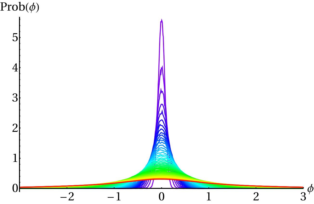
If there was no coupling between the flat and the non-flat directions, $\phi$ would freely fluctuate with an increasing variance $\langle\phi^{2}\rangle\sim NH_{o}^{2}$, until the non-renormalizable term $\phi^{6}/M_{p}^{2}$ would become important and equilibrium would be reached. The non-flat directions also fluctuate, obtaining variances of the order $\sim 0.1H_{o}^{2}$ in a matter of few efolds (bottom lines in Figure 2). Because of the coupling of $\phi$ to the fluctuations of non-flat directions $\chi_{i}$, the flat direction can then obtain an effective mass of order $\sim 0.1\lambda H_{o}$. Unless the couplings are very small, $\phi$ can no longer be considered as an effectively massless field in de Sitter space. As a consequence, its fluctuations will be blocked. This is demonstrated in Figures 1 and 2, which depicts the case $\lambda=g_{1}=g_{2}=1$.

In Figure 1 we show the evolution in time of the PDF of the flat directions. In Figure 2 we show the time evolution of the variance of each field. As can be clearly seen in the plots, it takes quite a long time, of the order of $\sim 1000$ e-folds, to reach a stationary regime. Once in this regime, the form of the flat direction PDF does not evolve in time anymore (red curves in Figure 1), and the variance growth stops, reaching a final asymptotic amplitude (see Figure 2). Note nevertheless, that during the first few tens of e-folds, the variance grows linearly with $N$, but still much more slowly than in the purely massless case. After the first hundred e-folds, the growth of the variance slows down and approaches the stationary regime. After $N\approx 1000$ efolds, the flat-direction finally enters into the stationary regime and its variance reaches an asymptotic constant amplitude $\left\langle\phi^{2}\right\rangle\approx 3.5H_{o}^{2}$, much smaller than the expected amplitude for a free massless field $\left\langle\phi^{2}\right\rangle=(N/4\pi^{2})H_{o}^{2}$.

In all of this, the non-renormalizable term plays no role, since the flat direction field never manages to fluctuate further than few units of $H_{o}$. For $\lambda=1$, the amplitude of the flat direction in the stationary regime, is $\sim\mathcal{O}(\sqrt{M_{p}/H_{o}})$ orders of magnitude smaller than the value needed for the non-renormalizable term to become relevant.

However, all this depends on the magnitude of the couplings. In Figure 3, we show the time evolution of the variance of the flat direction variance with different values of the Yukawa coupling $\lambda$, whilst $g_{1}=g_{2}=1$ as before. For $\lambda<\mathcal{O}(10^{-2})$, the flat-direction appears to fluctuate as one would expect from a massless field in de Sitter space. For $\lambda\sim\mathcal{O}(10^{-1})$, however, we already see some deviation from the purely massless case, since the flat-direction continues to grow for at least few thousand e-folds, albeit more slowly. For values of $\lambda$ between 0.1 and 1, we observe gradual blocking of the flat-direction fluctuations.

Thus, at the qualitative level, we may conclude that fluctuations within the F-term block the fluctuations along the flat directions that involve the third generation squarks and sleptons, while those involving only the first generation are likely to remain free to fluctuate. However, this is a conclusion based on the F-term alone and must be supplemented by the additional blocking provided by the D-term, as will be discussed in the next subsection.

We should like to stress that the PDF properties do not depend on the richness of the statistics. As can be seen in Figure 2, $n_{r}=10^{3}$ runs capture already all the essentials. There we show the evolution of the variance also for $n_{r}=10^{4},~10^{5}$ or $10^{6}$ independent runs, and all plots show the same behaviour, the only difference being that the richer the statistical sampling (i.e. the bigger $n_{r}$) the less noisy the plots are. As yet another check (not shown in the plots), we have compared the outputs from the same number of independent runs but different step size $dN$. We have found that if the simulation incorporates more than $100$ stochastic kicks per e-fold (i.e. if $dN<0.01$), the properties of the PDF remain the same as compared to the $dN=0.01$ case, no matter how small we make $dN$. For simulations with $n_{r}=10^{5}$ or more independent runs, we cannot even detect any difference between choosing $dN=0.01$ or $dN=0.001$.

Let us now focus on fluctuations within the D-terms. We set the F-term (i.e. the Yukawas) to zero and adopt the potential (12). We have thus two fields, $H$ and $L$, interacting with the coupling $g$, for which the configurations $H=\pm L$ represent a flat direction.

In Figure 4 we show the evolution of the variance of $L$ and $H$ for different strengths of the coupling between them. As in the case with an F-flat direction, we see again a gradual blocking in time of the freedom of these fields to fluctuate. The fluctuations of $H$ and $L$ are restricted more severely the stronger the gauge coupling. This can be observed in Figure 4, which shows the situation for the gauge couplings³³ 3 To be more precise, one should let the gauge couplings run to the scale of inflation $\sim\sqrt{HM_{p}}$. However, for our purposes, this would not change – qualitatively speaking – anything; the $U(1)$ and $SU(2)$ couplings would simply grow slightly, and thus the flat direction fluctuations in that case would result slightly more blocked, whereas although the $SU(3)$ coupling would indeed decrease, it would never become small enough for the flat direction to fluctuate as if it were a free massless field. of the (MS)SM, $g_{1}=0.35$, $g_{2}=0.62$ and $g_{3}=1.23$, for $U(1)_{Y}$, $SU(2)_{L}$ and $SU(3)_{c}$ interactions, respectively.

Of course the variance of $L$ or $H$ is not exactly the same as the variance of the flat direction, but still it gives a reliable measure about the freedom of the flat directions to fluctuate. To completely characterize the statistical properties of the flat directions, we should rather obtain instead the 2-dimensional PDF $\mathcal{P}(L,H)$, which describes the simultaneous distribution of both $H$ and $L$. In particular, $\mathcal{P}(L^{\prime},H^{\prime})dLdH$ represents the probability of finding $(L,H)$ within the field-space region $[L^{\prime},L^{\prime}+dL]\times[H^{\prime},H^{\prime}+dH]$. Therefore, similarly to the one-dimensional case, the $\mathcal{P}(L,H)$ function can be obtained from the numerics, simply by dividing the 2-dimensional unit-normalized histogrammatic distribution of the fields, at each time by the field bin steps $\Delta H$ and $\Delta L$.

In Figure 5 we show the evolution of the field fluctuations in the $(L,H)$ plane for all the (MS)SM gauge couplings, by plotting $\mathcal{P}(L,H)$ at different moments. One can clearly see the probability leaking into the flat directions $L=\pm H$. As expected from the behaviour of the variances shown in Figure 4, such leaking probability is of course higher the weaker the coupling. This is visualized in Figure 5, where we have fixed the scale in the horizontal to be same in all the snapshots taken at a given time for each different couplings. One can very clearly appreciate that the ’branches’ developing in $\mathcal{P}(L,H)$ along the flat directions, reach greater distances in the $(L,H)$ plane the weaker the gauge coupling is. For the $U(1)_{Y}$ case, the weakest of the (MS)SM couplings, the flat direction branches reach values as high as $12H_{o}$. But even in this case, in which the flat directions are the least constrained to fluctuate (compared to the $SU(2)_{L}$ and $SU(3)_{c}$ cases), such high amplitude regions are still highly unlikely. The 2-dim PDF obtained for the different coupling regimens are very suppressed for those high field values, if we compare them with the PDF for the case of a massless flat direction.

To assess the degree of blockage of the flat directions in the different coupling regimes, we show in Table 1 the probability of the fields to be above certain fixed thresholds. We then compare with the probability that one would expect for a massless non-interacting flat direction field. The numbers speak for themselves.

References

- [1] K. Enqvist and A. Mazumdar, Phys. Rept. 380, 99 (2003)
- [2] M. Grisaru, W. Siegel, and M. Rocek, Nucl. Phys. B 159, 429 (1979); N. Seiberg, Phys. Lett. B 318, 469 (1993) [arXiv:hep-ph/9309335].
- [3] T. S. Bunch and P. C. W. Davies, Proc. Roy. Soc. A360 (1978) 117.
- [4] A. Vilenkin, and L. H. Ford, Phys. Rev. D 26, 1231 (1982); A. D. Linde, Phys. Lett. B 116, 335 (1982); A. Vilenkin, Nucl. Phys. B 226, 527 (1983)
- [5] A. A. Starobinsky and J. Yokoyama, Phys. rev. D50 (1994) 6357.
- [6] M. Dine, L. Randall and S. Thomas, Nucl. Phys. B 458, 291 (1996).
- [7] T. Gherghetta, C. F. Kolda and S. P. Martin, Nucl. Phys. B 468 (1996) 37 [arXiv:hep-ph/9510370].
- [8] A. A. Starobinsky, In *De Vega, H.j. ( Ed.), Sanchez, N. ( Ed.): Field Theory, Quantum Gravity and Strings*, 107-126
- [9] K. -i. Nakao, Y. Nambu, M. Sasaki, Prog. Theor. Phys. 80 (1988) 1041.
- [10] J. M. Stewart, Class. Quant. Grav. 8 (1991) 909.
- [11] D. S. Salopek, J. R. Bond, Phys. Rev. D43 (1991) 1005-1031.
- [12] G. I. Rigopoulos, E. P. S. Shellard, JCAP 0510 (2005) 006. [astro-ph/0405185].
- [13] A. D. Linde, “Particle physics and inflationary cosmology”, arXiv:hep-th/0503203.
- [14] R. Allahverdi, K. Enqvist, J. Garcia-Bellido, A. Mazumdar, Phys. Rev. Lett. 97 (2006) 191304 [hep-ph/0605035]; R. Allahverdi, K. Enqvist, J. Garcia-Bellido, A. Jokinen, A. Mazumdar, JCAP 0706 (2007) 019 [hep-ph/0610134].
- [15] M. Matsumoto and T. Nishimura, ”Mersenne Twister: A 623-Dimensionally Equidistributed Uniform Pseudo-Random Number Generator”, ACM Transactions on Modeling and Computer Simulation, Vol. 8, No. 1, January 1998, pp 3-30.