Computability of the Julia set. Nonrecurrent critical orbits.
Abstract
We prove that the Julia set of a rational function is computable in polynomial time, assuming that the postcritical set of does not contain any critical points or parabolic periodic orbits.
1 Introduction.
A compact subset of the complex plane is called computable if it can be visualized on a computer screen with an arbitrarily high precision. Computer-generated images of mathematical objects play an important role in establishing new results. Among such images, Julia sets of rational functions occupy one of the most prominent position. Recently, it was shown that for a wide class of rational functions their Julia sets can be computed efficiently (see [6], [7], [21]) and yet some of those sets are uncomputable, and so cannot be visualized (see [8], [5]). Also, there are examples of computable Julia sets whose computational complexity is arbitrarily high (see [3]).
One of the natural open questions of computational complexity of
Julia sets is how large is the class of rational functions (in a
sense of Lebesgue measure on the parameter space) whose Julia set
can be computed in a polynomial time. Informally speaking, such
Julia sets are easy to simulate numerically.
Conjecture. The class of rational functions of degree
whose Julia set can be computed in a polynomial time
has a full measure in the space of parameters.
The main result of
the paper is the following.
Main Theorem. Let be a
rational function of degree . Assume that for each
critical point the -limit set does
not contain either recurrent critical point or a parabolic periodic
point of . Then the Julia set is computable in a polynomial
time.
As the reader will see below, this result can be viewed as
a natural step towards a proof of the conjecture.
The paper is organized as follows. In Section we give all necessary preliminaries in Computability and Complex Dynamics, state the results of the paper and discuss possible generalizations. To illustrate the results of the paper on a simple case in section we prove that for every subhyperbolic rational function the Julia set is computable in a polynomial time. In Section we prove the main result of the paper under a simplifying assumption that the rational map does not have any parabolic periodic points. In section we complete a proof of the main result.
Acknowledgements. It is my great pleasure to thank my supervisor Michael Yampolsky for posing the question of the paper and numerous fruitful discussions.
1.1 Preliminaries on computability
In this section we give a brief introduction to computability and complexity of functions and sets. The notion of computability relies on the concept of a Turing Machine (TM). A precise definition of a Turing Machine is quite technical and we do not give it here. For the definition and properties of a Turing Machine we refer the reader to [19] and [24]. The computational power of a Turing Machine is equivalent to that of a RAM computer with infinite memory. One can generally think about a Turing Machine as a formalized definition of an algorithm or a computer program.
There exist several different definitions of computability of sets. For discussion of different approaches to computability we refer the reader to [9]. In this article we use the notion of computability related to complexity of drawing pictures on a computer screen. Roughly speaking, a subset is called computable in time if there is a computer program which takes time to decide whether to draw a given square pixel in a picture of on a computer screen, which is accurate up to one pixel size. Before giving a rigorous definition of a computable Julia set we need to introduce some notations.
First we give the classical definitions of a computable function and a computable number.
Definition 1.
Let be countable subsets of . A function is called computable if there exists a TM which takes as an input and outputs .
Note that Definition 1 can be naturally extended to functions on arbitrary countable sets, using a convenient identification with .
Definition 2.
A real number is called computable if there is a computable function , such that for all
The set of computable reals is denoted by .
In other words, is called computable if there is an algorithm which can approximate with any given precision. The set is countable, since there are only countably many algorithms. The set of computable complex numbers is defined by . Note that both and considered with usual multiplication and addition form fields. Moreover, it is easy to see that is algebraically closed.
Let stand for Euclidian distance between points or sets in . Recall the definition of the Hausdorff distance between two sets:
where stands for the -neighborhood of :
We call a set a approximation of a bounded set if and . When we try to draw a approximation of a set using a computer program, it is convenient to let be a finite collection of disks of radius centered at points of the form for . Such can be described using a function
where and

Using this function, we define computability and computational complexity of a set in in the following way.
Definition 3.
A bounded set is called computable in time if there is a TM, which computes values of a function of the form (1.1) in time . We say that is poly-time computable if there exists a polynomial , such that is computable in time .
Similarly, one can define computability and computational complexity of subsets of . Moreover, definition 3 naturally extends to subsets of (see [9] Section 2.1). The Riemann sphere is homeomorphic to the unit sphere
Consider the stereographic projection
The inverse of this projection is given by
Observe that induces the spherical metric on , given by the formula
Definition 4.
A subset is called computable in time if is computable in time .
Proposition 5.
Let be a bounded subset. Then is computable as a subset of if and only if it is computable as a subset of . Similarly, is poly-time computable as a subset of if and only if it is poly-time computable as a subset of .
In this paper we discuss computability of the Julia sets of rational functions. For simplicity, consider the case of quadratic polynomials . By computing the Julia set of the map we mean the following problem:
However, an algorithm , computing , can handle only a finite amount of information. In particular, it can not read or store the entire input if . Instead, it may request this input with an arbitrary high precision. In other words, the machine has a command which for any integer requests the real and the imaginary part of a number , such that . It can be formalized using the notion of an oracle. Let
be the set of all dyadic numbers. Denote
the -th Cartesian power of . We will say that the open disk (respectively closed disk ) is dyadic if and are dyadic. Denote the set of all subsets such that can be represented as a finite union of dyadic disks.
Definition 6.
A function is called an oracle for an element if for all , where stands for the Euclidian norm in . An oracle Turing Machine is a TM, which can query for any .
The oracle is not a part of the algorithm, but rather enters as a parameter. In case of a computer program the role of the oracle is usually played by the user, who enters the parameters of the program. We should note also that an algorithm using an oracle require time units to read .
Now we are ready to define computability and computational complexity of the Julia set of a rational map.
Definition 7.
Let be a rational map. The Julia set is called computable in time if there is a Turing Machine with an oracle for the coefficients of , which computes values of a function of the form (1.1) for in time . We say that is poly-time computable if there exists a polynomial , such that is computable in time .
1.2 Hyperbolic maps
A rational map is called hyperbolic if there is a Riemannian metric on a neighborhood of the Julia set in which is strictly expanding:
for any and any tangent vector (see [18]). It follows that for a hyperbolic map there is a neighborhood of on which the metric induced by is strictly expanding:
Let be the spherical metric on the Riemann sphere. Then and are equivalent on a compact neighborhood of . One can deduce that there exists , and a neighborhood of , such that
Moreover, the last property is equivalent to the definition of hyperbolicity. Hyperbolic maps have the following topological characterization (see [18]).
Proposition 8.
A rational map is hyperbolic if and only if every critical orbit of either converges to an attracting (or a super-attracting) cycle, or is periodic.
Theorem 9.
For any there exists a Turing Machine with an oracle for the coefficients of a rational map of degree which computes the Julia set of every hyperbolic rational map in polynomial time.
To explain why this is an important result we would like to mention the following. It is known that hyperbolicity is an open condition in the space of coefficients of rational maps of degree . The famous conjecture of Fatou conjecture states that the set of hyperbolic parameters is dense in this space. This conjecture is known as the Density of Hyperbolicity Conjecture. It is the central open question in Complex Dynamics. Lyubich [16] and Graczyk-Swiatek [14] independently showed that this conjecture is true for the real quadratic family. Namely, the set of real parameters , for which the map is hyperbolic, is dense in .
1.3 Subhyperbolic maps
A rational map is called subhyperbolic if it is expanding on a neighborhood of the Julia set in some orbifold metric (see [18]). An orbifold metric is a conformal metric with a finite number of singularities of the following form. For each singularity there exists an integer index , such that for the branched covering the induced metric
in -plane is smooth and nonsingular in a neighborhood of the origin. Douady and Hubbard proved the following (see [18])
Proposition 10.
A rational map is subhyperbolic, if and only if every critical orbit of is either finite or converges to an attracting (or a super-attracting) cycle.
For a subhyperbolic map, the corresponding orbifold has singularities only at postcritical points, which lie in . In presence of these singularities the algorithm, which works in the case of hyperbolic maps, can not be applied directly for subhyperbolic maps. We show in this paper how to change this algorithm to compute the Julia set of a subhyperbolic map in a polynomial time. One of the results of this paper is the following theorem.
Theorem 11.
There is a TM with an oracle for the coefficients of a rational map , such that for every subhyperbolic map the machine computes in polynomial time, given some finite non-uniform information about the orbits of critical points of .
We will specify later, which non-uniform information does use.
1.4 The main results: nonrecurrent critical orbits.
Let be a rational map. For a point denote
the forward orbit of . Let be the -limit set of . Denote the set of critical points of which lie in . Put
Our main result is devoted to the class of rational maps without recurrent critical points. Namely, we prove here the following:
Theorem 12.
Let be a rational map. Assume that has no parabolic periodic points and does not contain any critical points. Then is poly-time computable by a TM with an oracle for the coefficients of .
Although in this case there is no guarantee that any kind of expansion holds on the whole Julia set of , the following well-known theorem of Mañé (see [17],[23]) implies that there is expansion on the closure of the postcritical set of .
Theorem 13.
Let be a rational map. Let be a compact invariant set, such that does not contain any critical points of or parabolic periodic points and for any recurrent critical point of . Then there exists , such that for any .
As we see, the theorem of Mañé gives expansion only near the points, whose forward orbits are isolated from the parabolic periodic points. The question arises: is it possible to generalize Theorem 12 for the maps with parabolic periodic points? It is known that the algorithms, used for computing hyperbolic Julia sets, require exponential time in the presence of parabolic points (see [18], app. H). However, in the paper [7] (see also [9]) Braverman proved that for any rational function , such that every critical orbit of converges either to an attracting or to a parabolic orbit, the Julia set is poly-time computable. Combining the algorithm used in [7] with the algorithm, which we use in the present paper to prove Theorem 12, we obtain the following generalization of Theorem 12:
Theorem 14.
Let be a rational map. Assume that does not contain neither critical points nor parabolic periodic points. Then is poly-time computable by a TM with an oracle for the coefficients of .
1.5 Possible generalizations.
In this subsection we discuss possible generalizations of the results of this paper. First we would like to mention that the algorithm which we use to prove Theorem 14 cannot be applied to compute the Julia set of a rational map , such that contains a parabolic periodic point. However, we believe that the following statement is true.
Conjecture 15.
Let be a rational map. Assume that does not contain any critical points. Then is poly-time computable by a TM with an oracle for the coefficients of .
Another important class of rational maps is the class of Collet-Eckmann maps.
Definition 16.
Let be a rational map. Assume that there exist constants such that the following holds: for any critical point of whose forward orbit does not contain any critical points one has:
| (5) |
Then we say that the map is Collet-Eckmann (CE). The condition is called the Collet-Eckmann condition.
In [2] Avila and Moreira showed that for almost every real parameter the map is either Collet-Eckmann or hyperbolic. In [1] Aspenberg proved that the set of Collet-Eckmann maps has positive Lebesgue measure in the parameter space of all rational maps of fixed degree . Moreover, there is a conjecture that for almost all rational maps in this space the following is true:
- 1)
the forward orbit of every critical point either is finite or converges to an attracting periodic orbit;
- 2)
for any critical point either there exists such that for any or the forward orbit of contains another critical point.
By the theorem of Mañé 13, every rational map such that does not contain neither critical points nor parabolic periodic points is Collet-Eckmann. We believe that the following generalization of Theorem 14 is true.
Conjecture 17.
Let be a rational map such that the conditions and above are satisfied. Then is poly-time computable by a TM with an oracle for the coefficients of .
Thus, we conjecture that
Conjecture 18.
For almost all rational maps of degree is poly-time computable.
2 Poly-time computability for subhyperbolic maps.
In this section we prove Theorem 11. Namely, we construct an algorithm which for every subhyperbolic rational map computes in polynomial time. The algorithm uses the coefficients of the map and some non-uniform information which we will specify in the following subsection.
2.1 Preparatory steps and non-uniform information.
In this paper we actively use the classical Koebe distortion theorem (see [10]). Let us state it here. For denote
Theorem 19.
Let be a univalent function. Then for any one has:
| (6) | |||
| (7) |
The statement (7) of the Koebe distortion theorem can be reformulated the following way. Let , , . Then
| (8) |
We will also use Koebe One-Quarter Theorem, which can be derived from Koebe Distortion Theorem.
Theorem 20.
Suppose is a univalent function. Then the image contains the disk of radius centered at .
Fatou and Julia proved the following fundamental result.
Theorem 21.
Let be a rational map of degree . Then the immediate basin of each attracting cycle contains at least one critical point. In particular, the number of attracting periodic orbits is finite and do not exceed the number of critical points.
Proposition 22.
Let be a complex polynomial. There exists a TM with an oracle for the
coefficients of and a natural number as an input, such that outputs a finite
sequence of complex dyadic numbers for which:
each
lies at a distance not more than from some root of ;
each root of
lies at a distance not more than from one of .
Denote and the number of critical points of which lie in the Fatou set and the Julia set of correspondingly. The algorithm computing the Julia set of a subhyperbolic map will use the numbers
| (9) |
as the non-uniform information.
Observe that the assertions and are equivalent. Indeed, by Proposition 10 if then there is at least one attracting (or superattracting) periodic point and the Fatou set is nonempty. On the other hand if the Fatou set is nonempty, then there is at least one attracting (or superattracting) periodic point. The basin of this periodic point contains a critical point. Thus if , then the problem of computing is trivial. Therefore, we will assume that and .
Also, without loss of generality we may assume that . Indeed if , then using Proposition 22 we can find a dyadic point which lie in the Fatou set of . Let be a Möbius map such that . Consider the map instead of .
Proposition 23.
Let be a subhyperbolic rational map. There exists a
Turing Machine with an oracle for the coefficients of
such that the following is true. Given the number of
critical points outputs a dyadic set
such that
all the attracting and super attracting orbits of belong to ,
for
any the orbit of converges to an attracting periodic orbit,
.
Proof.
The algorithm works as follows. Initially, let be an empty collection of dyadic disks. At -th step, , do the following. By Proposition 22 there is an algorithm which finds all periodic points of of period at most with precision . Let be approximate position of a periodic point of period . The corresponding periodic point belongs to the disk . Consider the disk . If does not intersect neither one of the disks from , then approximate the image by a dyadic set with precision . Namely, find a set such that
Verify if
| (10) |
This would imply that
| (11) |
In this case, compute dyadic sets , such that and for each , where is taken modulo . Add dyadic sets to the collection .
Next, calculate approximations of the images of critical points of such that . If there are of the points , such that
then we stop the algorithm and output . Otherwise, go to step .
Let us show that the algorithm eventually stops and outputs a set , satisfying the conditions of Proposition 23. Let be an attracting (or super-attracting) periodic point of period with multiplier . Let . Then for small enough one has
It follows that for some the corresponding approximation of and the set satisfy the property (10). On the other hand if (11) holds, then by Schwartz Lemma contains an attracting periodic point, whose basin contains . Therefore if the algorithm runs sufficient amount of steps, the union of dyadic sets from satisfies the condition of the Proposition 23.
By Proposition 10, the orbit of each critical point of which does not lie in converges to an attracting periodic orbit. Thus, for some there will be of the points , belonging to . This implies, then the algorithm stops. By Theorem 21, we obtain that contains all attracting periodic orbits of . Notice that conditions and of the Proposition 23 for this set are satisfied by construction. ∎
Denote the set of critical points of which lie in the Fatou set of . Put
The next statement is a subhyperbolic analog of Proposition 3.7 from [9].
Proposition 24.
There exists an algorithm which, given the coefficients of a subhyperbolic rational map of degree and the number , outputs a planar domain such that:
- (1)
,
- (2)
,
- (3)
.
Proof.
First use the algorithm from Proposition (23) to find a dyadic set satisfying to the conditions of Proposition 23. Let . We can algorithmically construct a dyadic set such that
Compute a dyadic number such that
Also, compute dyadic approximations of critical points of such that
By Theorem 10, for any critical point we will eventually have:
Therefore, for large enough , the set will contain of the points . Take such . Then for any one has
Thus, . Compute a dyadic set such that
Clearly, for the set conditions hold. ∎
2.2 Construction of the subhyperbolic metric.
Here we give the construction of a subhyperbolic metric (see [18]). We modify the construction from [18] to be able to write it as an algorithm. First we recall the definition and basic properties of an orbifold. We refer the reader to [18] for details.
Definition 25.
An orbifold is a Riemann surface together with a function such that the set is discrete. Points for which are called branch points.
Definition 26.
Let be a subhyperbolic rational map. An orbifold metric on a neighborhood of is called subhyperbolic if is strictly expanding on with respect to :
for any except the branch points.
Let be a regular branched covering. Then for every the local degree of at a point does not depend on . One can define the weight function of the covering assigning the local degree of at .
Definition 27.
Let be an orbifold. A regular branched covering
with the weight function such that is simply connected is called a universal covering of the orbifold . We will use the notation for a universal covering of this orbifold.
Proposition 28.
Let be an orbifold. The universal covering
exists and unique up to conformal isomorphism, except in
the following two cases:
(the Riemann sphere) and
has only one branch point;
and has two branch points such that
.
The Euler characteristic of an orbifold is the number
Since the set of branch points of is discrete the last sum contains at most countable number of nonzero terms. If contains infinitely many branch points then we set . The orbifold is called hyperbolic if .
Lemma 29.
If is a hyperbolic orbifold then conformally isomorphic to the unit disk.
Let be a subhyperbolic rational map. Let be the set from Proposition 24. Construct an orbifold in the following way. Put . Denote the set of the critical points of which lie in . As the set of branch points of take . Since is subhyperbolic, is finite. Put for all . Denote the local degree of at . Define numbers such that the following condition holds:
| (12) |
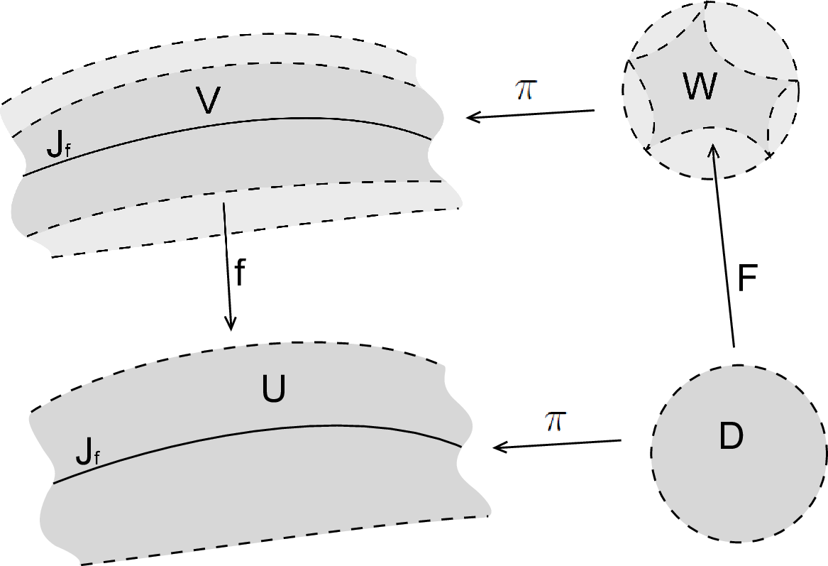
If the orbifold that we obtained is not hyperbolic, take any repelling orbit of of the length at least and replace with for all from this orbit. The new orbifold will be hyperbolic and satisfying the condition (12).
By Proposition 28 there exists a universal covering
By Lemma 29, without loss of generality we may assume that is the open unit disc. Since , Condition (12) guarantee that the map lifts to a holomorphic map
Note that is strictly contained in . Denote the Poincaré metric on . By the Schwartz-Pick Theorem, the map is strictly decreasing in the metric . Let be the projection of onto . For any and one has:
| (13) |
It follows that the map is strictly expanding with respect to the norm induced by . To show that the metric is subhyperbolic we need to prove that is uniformly strictly expanding. First we will prove an auxiliary lemma.
Lemma 30.
There exist a constant such that for any except the branch points of the orbifold one has:
where are the branch points. The constant can be obtained constructively.
Proof.
Let . Assume that is not a branch point. To estimate without loss of generality we may assume that . Recall that the Poincaré metric on the unit disk is of the form:
Therefore one has:
We can construct a dyadic number such that is contained in a disk of radius . By Schwartz Lemma,
Thus,
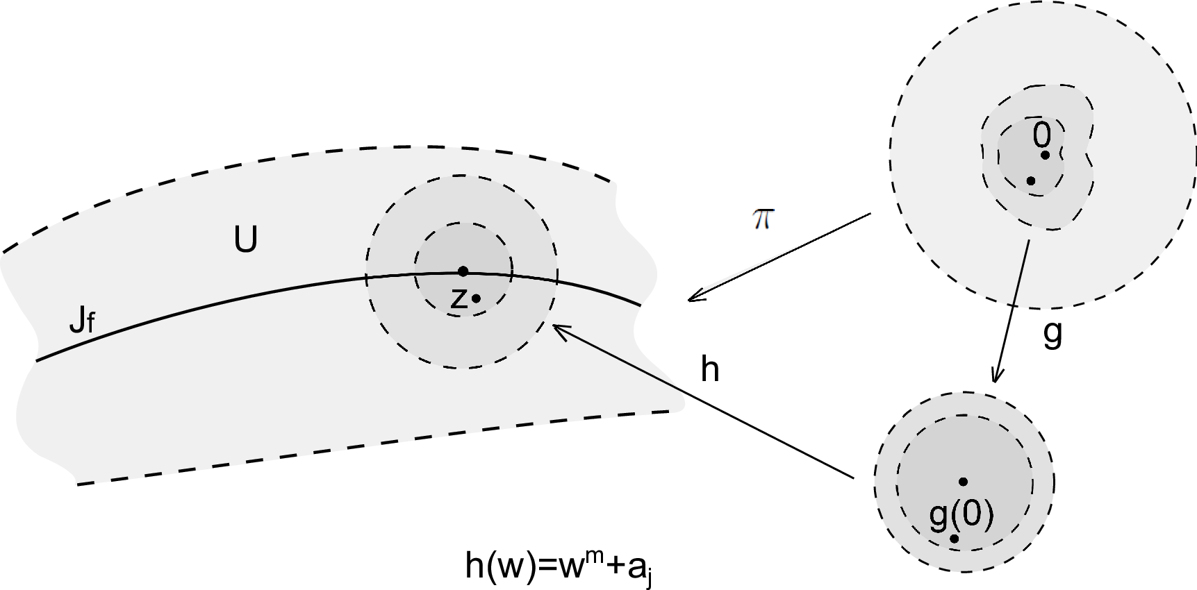
Recall that the set of branch points consists of critical points which lie in and possibly one repelling periodic orbit. It follows from Proposition 22 that we can construct a dyadic number such that disks are pairwise disjoint and all belong to . Assume first that . Considering the branch
of such that , by Schwartz Lemma we obtain
Let for some . Then in a neighborhood of the map can be written in the form
where is a one to one map from onto with . In one has
| (14) |
Consider the map Since
by Schwartz Lemma we get:
where constant can be obtained constructively. Now (14) implies
which finishes the proof. ∎
Proposition 31.
There exists a constant such that
for any . The constant can be constructed algorithmically.
Proof.
For a map between two hyperbolic Riemann surfaces denote
the magnitude of the derivative of computed with respect to the two Poincaré metrics. Denote the distance in the metric on and the distance in the Poincaré metric on . Let
be the inclusion map. Then we have:
Using Lemma 30 it is not hard to show that we can construct a dyadic constant such that
Let . Then there exists and such that
A suitable fractional linear transformation sends to and to . Explicit calculations show that
| (15) |
Now, by Schwartz-Pick Theorem
| (16) |
The right hand side of the last inequality can be estimated explicitly. It is equal to
Note that increases with . By (15) and (16) the value is bounded from above with for . By (13) we obtain that for is bounded from below with . ∎
Corollary 32.
The metric is subhyperbolic.
2.3 The algorithm.
Denote . Notice that
for any . Let us prove the following auxiliary statement.
Proposition 33.
There is an algorithm computing two dyadic constants such that for any and any if then one has
Proof.
First construct a dyadic number such that
Then for any , satisfying to the conditions of the proposition, the open disk does not intersect neither nor a forward orbit of a critical point of . Let
be the branch of such that . Then by Koebe Quarter Theorem the image contains the disk or radius Since is invariant under it follows that
Set .
Further, denote
| (17) |
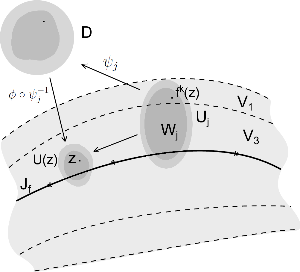
Notice that is finite. Recall that we can algorithmically construct approximate positions of all critical points of which lie in with any given precision. Thus, we can approximate . We can also algorithmically construct positions of some points in which lie apart from with any given precision. For instance, using the algorithm from Proposition 22 we can calculate approximate position of a repelling periodic orbit. Using the above we can construct a finite number of pairs of simply connected dyadic sets such that the following is true
-
for any ;
-
;
-
.
For each fix the Riemann mapping . Assume now that satisfy the conditions of the proposition. Then for some . Let be the branch of such that . Consider the map
Notice that . Applying both parts of Theorem 19 to the map , we can construct a dyadic number not depending either on or on such that is contained in the disk of radius centered at . It follows that
Set . ∎
As a preparatory step construct a dyadic set such that
Compute dyadic numbers such that
| (18) |
Let . Lemma 30 implies that for any
| (19) |
Let stand for the logarithm with base 2. We will use the standard notation for the integer part of a real number .
Assume that we would like to verify that a dyadic point is close to . Consider first points which lie outside . Construct a dyadic set such that
Then we can approximate the distance from a point to by the distance form to up to a constant factor.
Now assume . Consider the following subprogram:
while
do
Compute dyadic approximations
with precision
.
Check the inclusion
:
-
if , go to step ;
-
if , proceed to step ;
Check the inequality . If true, output and exit the subprogram, otherwise
output and exit subprogram.
end while
Output end exit.
end
The subprogram runs for at most number of while-cycles each of which consist of a constant number of arithmetic operations with precision dyadic bits. Hence the running time of the subprogram can be bounded by using efficient multiplication.
Proposition 34.
Let be the output of the subprogram. Then
where ,
Proof.
Now, to distinguish the case when from the case when we can partition each pixel of size into pixels of size and run the subprogram for the center of each subpixel. This would increase the running time at most by a constant factor.
3 Maps without recurrent critical orbits and parabolic periodic points.
In this section we will prove Theorem 12. Throughout this section let stand for a rational map without parabolic periodic points such that does not intersect the set of critical points of .
3.1 Preparatory steps and nonuniform information.
As in the case of subhyperbolic map, without loss of generality we will assume that . For any put
Put . Denote
By our assumptions, there are no either recurrent critical orbits or parabolic periodic points of , the set is invariant and does not contain critical points of . Thus, the set satisfies the conditions of Mañé’s Theorem . The following result is classical (see [18]).
Theorem 35.
Let be a rational map. Then the boundary of each cycle of Siegel disks and each cycle of Herman rings belongs to (see (17)).
Lemma 36.
There are no either Siegel disk cycles or Herman ring cycles in the Fatou set of .
Proof.
Assume for simplicity that there is a Siegel disk . By replacing with an iterate if necessary, we can assume that . Then the boundary of the Siegel disk is forward invariant under and belongs to . It follows that does not contain any critical point of . Thus, satisfies the condition of Mañé’s Theorem . Therefore, there exists such that is expanding on a neighborhood of . This is impossible since is conjugated to a rotation inside . The other case can be treated similarly.∎
To compute the Julia set the algorithm will use the following non-uniform information:
and degrees
of the critical points of which lie in
;
, dyadic numbers
and a dyadic set such that
and for any one has
In this section we will prove the following theorem.
Theorem 37.
Let be a rational map such that has no parabolic periodic points and does not contain any critical points. There exists a Turing Machine which, given an oracle for the coefficients of the map and the non-uniform information , computes in a polynomial time.
Now we prove several auxiliary lemmas.
Lemma 38.
For any and any one has
Notice that, in particular, the restriction of on is one to one for any .
Proof.
Using Lagrange formula
| (24) |
for we obtain
∎
For simplicity set . Lemma 38 implies that
| (25) |
Lemma 39.
For any and one has
| (26) |
Proof.

Let satisfy the conditions of Lemma 39. Put
By Lemma 38, is univalent on for each and
It follows that there exists , such that
and is univalent on . Lemma 38 implies that
Let such that is identical on . Put
Then . By Koebe Distortion Theorem (see (8)), one has:
| (27) |
Since is invariant under , it follows that
| (28) |
Since , is equivalent to the first part of . Similarly, one can prove the second part of . Observe that we can not prove a lower bound for in this way since is not necessarily invariant under .∎
Till the end of this section in each of the preceding statements we assume that the Turing Machine has an access to the non-uniform information and an oracle for the coefficients of the map .
Lemma 40.
There exists a TM which computes dyadic numbers , such that for any critical point of which lie in one has
for any , where is the degree of at .
Proof.
By Proposition 22 we can find approximate positions of all critical points of . Notice that the orbit of every critical point of which lie in the Fatou set converges to an attracting cycle. Using the ideas from the proof of Proposition 23 we can distinguish the critical points which belong to the Fatou set from the critical points which belong to the Julia set. Let be a critical point of degree . Then we can approximate the coefficient at in the Taylor expansion of at and compute , such that
for any . Let be any -th root of . Then there exists a unique holomorphic map from to a neighborhood of the origin, such that
Make smaller if necessary in order to have
The image contains a disk , where can be algorithmically constructed. Let , such that
Take . Observe that
Let , such that
Then . There exists , such that . One has
Let be the number for which takes the closest value to . From simple geometric observations it follows that
for any . Since , it follows that
where . ∎
Using the definition of the dyadic set and Proposition 22 one can prove the following statement.
Lemma 41.
There exists a TM which
computes a dyadic number such
that
| (29) |
Proposition 42.
There exists a TM which computes dyadic number such that the following is true. For any and one has
Proof.
First put . Let . Set
where . Using Lemma 39, we obtain:
| (30) |
Let . Put . Let be the degree of at . Then we can algorithmically construct a dyadic number , such that
for any . Then
| (31) |
Lemma 40 implies that we can algorithmically construct dyadic numbers such that
| (32) |
for any . Combining with , we get
| (33) |
for any .
A direct analog of the Proposition 24 holds for the maps , which satisfy the conditions of Theorem 12.
Proposition 43.
Let be a rational map such that does not have any parabolic periodic points and does not contain any critical points of . There exists a TM which given an oracle for the coefficients of the map and the non-uniform information outputs a planar domain such that:
- (1)
,
- (2)
,
- (3)
.
Denote
If then is hyperbolic. Since for hyperbolic maps poly-time computability of the Julia set is well known (see [6] and [21]), we will assume that . Then is strictly smaller than . It follows that is strictly larger than . Let stands for the hyperbolic norm associated with . Then
Let be the metric on induced by . It follows that
| (35) |
Notice that
One can construct a dyadic subset , such that
Denote .
Lemma 44.
One can algorithmically construct dyadic numbers , such that
- (1)
for any ;
- (2)
for any ;
- (3)
.
Notice that the Euclidian metric and the hyperbolic metric are equivalent on any compact subset of . The following lemma can be proven similarly to Lemma 30.
Lemma 45.
One can algorithmically construct a dyadic constant such that
| (36) |
for any .
Lemma 46.
There exists a TM which computes dyadic numbers such that for any and one has .
Proof.
Since does not have parabolic periodic orbits one has
Therefore there exist such that for any and
Make smaller if necessary in order to have
Let . Assume there exists such that
Let be the minimal such number. Then
It follows from Lemma 40 that one can compute dyadic numbers , such that
| (37) |
for any and . Put . Denote inductively and as follows:
while , where
Now by (35), Lemma 44 and Proposition 42 the following is true:
- 1)
for any ;
- 2)
if , then
- 3)
if and , then
- 4)
if and , then
- 5)
if and , then
- 6)
if and , then
The items are direct corollaries of the choice of the dyadic constants, formula (35), Lemma 44 and Proposition 42. Let us proof . Let
If , then follows directly from . Otherwise denote the remainder of modulo . Then by and (25)
Let be the number of -th, for which
If
then let
be the minimal and be the maximal such .
case 1: . Then one of the following two possibilities holds.
a) . Then . By ,
b) . Then by and ,
case 2: . There are two possibilities.
a) . Then . As in the case 1,
b) . Then, by and , . By ,
| (43) |
Among the numbers there is at most one number such that
and at most one number such that
It follows that
| (44) |
where
Theorem 47.
There exists a TM which computes the coefficients of a polynomial such that for any with one has
Proof.
Let and . Let be the maximal number, such that
Construct as in Lemma 46. Then properties hold. Let be as in Lemma 46 and be the sequence of indexes for which
Then, by Lemma 45 and properties and from Lemma 46,
It follows that
Let be an index such that and . Let
It follows from Lemma 46 that
Therefore,
for some number which can be obtained algorithmically. Now it is easy to see that among any consecutive integer numbers between and there exist such that
It follows that
Since , this finishes the proof.∎
3.2 The algorithm.
Similarly to Proposition 33 one can prove the following result.
Proposition 48.
There is an algorithm computing two dyadic constants such that for any and any if then one has
Now we are ready to describe the algorithm. The steps of the algorithm are analogous to the steps of the corresponding algorithm for a subhyperbolic map. Compute dyadic numbers such that
| (45) |
Assume that we would like to verify that a dyadic point is close to . Construct a dyadic set such that
Then we can approximate the distance from a point to by the distance form to up to a constant factor.
Now assume that . Let be the polynomial
from Proposition 47.
Similarly to the case of a subhyperbolic map, consider the
following subprogram:
while
do
Compute dyadic approximations
with precision
.
Check the inclusion
:
-
if , go to step ;
-
if , proceed to step ;
Check the inequality . If true, output and exit the subprogram, otherwise
output and exit subprogram.
end while
Output end exit.
end
The subprogram runs for at most number of while-cycles each of which consist of a constant number of arithmetic operations with precision dyadic bits. The following proposition is proved in the same way as Proposition 34.
Proposition 49.
Let be the output of the subprogram. Then
where ,
4 Maps with parabolic periodic points.
In this section we will sketch the proof of Theorem 14. Let be a rational map such that does not contain either critical points or parabolic periodic points. We will assume that the periods and multipliers of the parabolic periodic points are given as a part of the non-uniform information. Replacing with some iteration of if necessary, we may assume that the multiplier and the period of each of the parabolic periodic points is equal to . Then at each parabolic periodic point (in fact, a fixed point) the map can be written in the form
where . We will assume that the numbers are also given as a part of the non-uniform information. Observe that some parabolic fixed points of may belong to the postcritical set of .
In this section we denote by the set of critical points such that the forward orbit does not contain any parabolic periodic points and by the set of critical points such that an iteration of hits a parabolic fixed point. Let be the same as in section 3. For numbers , a direction and a point introduce a sector
| (50) |
Let be
all parabolic fixed points of . The algorithm will use the same
non-uniform information which was described in
subsection 3.1 and, in addition,
approximate positions of with a dyadic
precision and a number
such that for each :
is a unique fixed point of in
(and thus can be approximated
efficiently using Newton method);
for each critical point which lie in one has

for each attracting direction at the sector
belongs to an attracting Fatou petal at ,
and the set
belongs to the union of the repelling petals at . Observe that for a point in the sector the distance up to a constant factor can be approximated by . We will use the following result from [7] (see Lemma ).
Lemma 50.
Let be given as a power series with radius of convergence . There is an algorithm which given a point with computes -th iteration of and the derivative with precision in time polynomial in and . Here is some dyadic constant which can be algorithmically constructed. The algorithm uses an oracle for the coefficients .
Lemma 50 implies that we can compute ”long” iterations of points close to parabolic periodic points efficiently.
By the assumptions on the map one can algorithmically construct a dyadic number such that the following is true. Let a point be -close to the Julia set. Assume that some iteration belong to . Consider the neighborhood . Let
be the pullbacks of under along the orbit of , where is a neighborhood of . Then the number of for which contains a critical point is bounded from above by a constant independent from and . In a similar fashion as Proposition 33 using ideas of Lemma 40 we can prove the following statement.
Proposition 51.
We can algorithmically construct dyadic numbers such that for each if satisfies the following
for some parabolic fixed point then
From the description of the dynamics near a parabolic point using Koebe Theorem 19 we can obtain the following result.
Proposition 52.
One can algorithmically construct numbers such that for each and each if
then one has and
Now we briefly
explain how to adopt the algorithm from Paragraph
3.2 to prove Theorem 14. Assume
that we want to verify if a point is -close to
. Construct a sequence in a way
analogues to the construction from Lemma 46
(see (3.1)). We will define in a
different way from (3.1) only if for some parabolic fixed point .
In this case we do the following.
If for some attracting direction
then we stop. We can find the distance from to
up to a constant factor. Using Proposition 51 we can estimate the distance from to
up to a constant factor.
If then
consider the points , where . Observe
that by Lemma 50 we can find a
approximation of in time polynomial in and .
Let be the minimal nonnegative integer number such that
Set .
Observe that a direct analog of Theorem 47 is not true in a presence of parabolic periodic points, even if we assume that does not belong to an attracting basin of a parabolic periodic point. For a point close to a parabolic fixed point in a repelling petal it takes exponential time in to escape an -neighborhood of the parabolic fixed point. However, using Lemma 50 and Proposition 52 we can prove the following.
Proposition 53.
There is an algorithm computing coefficients of a polynomial such that if
then . Moreover, we can compute -approximations of and for in time polynomial in .
Now we briefly describe the algorithm
computing the Julia set in a polynomial time in . Let . Assume that we want to verify that is
close to . Without loss of generality we may assume
that . Compute approximate values of
and of with precision ,
.
If for some
such that
then we can find approximate distance from to . By
Proposition 51, we can find up to some
constant.
If for some , then
we can find the distance up to a constant factor. Using
Koebe Theorem we can find the distance
from to up to a constant factor.
If neither nor holds then by Proposition
53
In conclusion, let us mention an alternative numerical method to calculate iterations of points close to parabolic periodic orbits. This method has been implemented in recent literature. To illustrate the method we consider a map with a simple parabolic point at the origin:
Let and be the germ at infinity given by
Denote by the unit shift: . In [12] and [13] Ecalle has shown the following
Theorem 54.
The equation has a unique formal solution in terms of the series (generally, divergent)
| (51) |
The series gives an asymptotic expansion for an attracting and a repelling Fatou coordinates of the map , and correspondingly.
For survey on divergent series and asymptotic expansions we refer the reader to [20]. Theorem 54 means that the Fatou coordinates and near infinity can be approximated by finite sums of the series (51). To approximate -th iteration of the map near the origin one can use the following formula:
where stands for either or depending on whether belongs to an attracting or a repelling Fatou petal of . We would like to emphasize that this is not a rigorous method since we do not know how many terms of the series (51) to take to obtain the desired precision. However, empirically, the asymptotic expansion (51) approximates the Fatou coordinates with a very high precision. For instance, in [15] Lanford and Yampolsky used the series in their computational scheme for the fixed point of the parabolic renormalization operator. Our work in progress [11] give us a reason to hope that the described method can be made rigorous.
References
- [1] M. Aspenberg, The Collet-Eckmann condition for rational functions on the Riemann sphere, Ph.D. Thesis, KTH, Sweden, 2004.
- [2] A. Avila, C.G. Moreira, Statistical properties of unimodal maps: the quadratic family, Annals of Mathematics, 161, no. 2 (2005), 831-881.
- [3] I. Binder, M. Braverman, M. Yampolsky, On computational complexity of Siegel Julia sets, Commun. Math. Phys. 264 (2006), no. 2, 317-334
- [4] I. Binder, M. Braverman, M. Yampolsky, Filled Julia sets with empty interior are computable, Journ. of FoCM, 7 (2007), 405-416.
- [5] I. Binder, M. Braverman, M. Yampolsky, Constructing locally connected non-computable Julia sets, Commun. Math. Phys. 291 (2009), 513-532.
- [6] M. Braverman, Computational complexity of Euclidian sets: Hyperbolic Julia sets are poly-time computable, Master’s thesis, University of Toronto, 2004.
- [7] M. Braverman, Parabolic Julia sets are polynomial time computable, Nonlinearity 19, (2006), no.6, 1383-1401.
- [8] M. Braverman, M. Yampolsky, Non-computable Julia sets, Journ. Amer. Math. Soc. 19 (2006), no. 3, 551-578.
- [9] M. Braverman, M. Yampolsky, Computability of Julia sets, Series: Algorithms and Computation in Mathematics, Vol. 23, Springer, 2008.
- [10] J. B. Conway, Functions of one complex variable , Springer-Verlag, New York, New York, 1995.
- [11] A. Dudko, D. Sauzin, Ecalle-Voronin invariants via resurgence and mould calculus, in preparation.
- [12] J. Écalle. Les fonctions résurgentes, Vol. 1. Publ. Math. d’Orsay 81-05, 1981.
- [13] J. Écalle. Les fonctions résurgentes, Vol. 2. Publ. Math. d’Orsay 81-06, 1981.
- [14] J. Graczyk, G. Swiatek, Generic hyperbolicity in the logistic family, Ann. of Math., v. 146 (1997), 1-52.
- [15] Oscar Lanford III, M. Yampolsky, The fixed point of the parabolic renormalization operator, arXiv:1108.2801.
- [16] M. Lyubich, Dynamics of quadratic polynomials, I-II. Acta Math., 178 (1997), 185-297.
- [17] R. Mañé, On a Theorem of Fatou, Bol. Soc. Bras. Mat., Vol. 24, no. 1, 1993, pp. 1-11.
- [18] J. Milnor, Dynamics in one complex variable. Introductory lectures, 3rd ed., Princeton University Press, 2006.
- [19] C. M. Papadimitriou, Computational complexity, Addision-Wesley, Reading, Massachusetts, 1994.
- [20] J.-P. Ramis. Séries divergentes et théories asymptotiques, Panoramas et Synthèses (1994).
- [21] R. Rettinger, A fast algorithm for Julia sets of hyperbolic rational functions, Electr. Notes Theor. Comput. Sci. 120 (2005), 145-157.
- [22] D. Sauzin, Resurgent functions and splitting problems, RIMS Kokyuroku 1493, (2005), 48-117, available from http://www.imcce.fr/Equipes/ASD/person/Sauzin/sauz preprint.php
- [23] M. Shishikura, Tan Lei, An alternative proof of Mane’s theorem on non-expanding Julia sets, in “The Mandelbrot set, Theme and Variations”, Ed. Tan Lei, London Math. Soc. Lect. Note Ser. 274, Cambridge Univ. Press, 2000, p.265-279.
- [24] M. Sipser, Introduction to the theory of computation, second edition, BWS Publishing Company, Boston, 2005.
- [25] H. Weyl, Randbemerkungen zu Hauptproblemen der Mathematik, II, Fundamentalsatz der Algebra and Grundlagen der Mathematik, Math. Z. 20(1924), 131-151.