R-parity Conservation via the Stueckelberg Mechanism:
LHC and Dark Matter Signals
Abstract
We investigate the connection between the conservation of R-parity in supersymmetry and the Stueckelberg mechanism for the mass generation of the vector gauge boson. It is shown that with universal boundary conditions for soft terms of sfermions in each family at the high scale and with the Stueckelberg mechanism for generating mass for the gauge boson present in the theory, electric charge conservation guarantees the conservation of R-parity in the minimal extended supersymmetric standard model. We also discuss non-minimal extensions. This includes extensions where the gauge symmetries arise with an additional , where is a hidden sector gauge group. In this case the presence of the additional allows for a gauge boson mass with interactions to lie in the sub-TeV region overcoming the multi-TeV LEP constraints. The possible tests of the models at colliders and in dark matter experiments are analyzed including signals of a low mass resonance and the production of spin zero bosons and their decays into two photons. In this model two types of dark matter candidates emerge which are Majorana and Dirac particles. Predictions are made for a possible simultaneous observation of new physics events in dark matter experiments and at the LHC.
I Introduction
R-parity is an important symmetry in supersymmetric theories (For a review see [1]). In supergravity theories [2], over most of the parameter space of models consistent with the radiative breaking of the electroweak symmetry, the lightest neutralino is found to be the lightest supersymmetric particle, and this, along with R-parity (defined as , where , and stand for the spin, baryon number and lepton number, respectively) and charge neutrality allows for the lightest neutralino to be a promising candidate for cold dark matter as suggested in [3].
The question then, is, if indeed R-parity turns out to be a conserved symmetry of nature, how does such a symmetry come about, and how one may guarantee that it is conserved. It is known that the MSSM with the inclusion of a right handed neutrino, one for each generation, has an anomaly free which can be gauged11 1 A gauged arises naturally in GUT models such as and and in string models.. Of course, a gauge boson must grow mass otherwise it would produce an undesirable long range force. In the analysis that follows it is shown that a gauged symmetry, where the gauge boson develops a mass through the Stueckelberg mechanism extending the Standard Model gauge group [4] [5, 6] preserves R-parity, i.e., R-parity does not undergo spontaneous breaking by renormalization groups effects under the assumption of universality of soft scalar masses, charge conservation and in the absence of a Fayet-Iliopoulos D-term. We will later refer to this model as the Minimal Stueckelberg Extension of the MSSM.
The fact that the minimal gauged model proposed in this work preserves R-parity, with mass growth arising from the Stueckelberg mechanism, is in contrast to models with a gauged where the symmetry is broken spontaneously and thus does not necessarily preserve the R-parity invariance. Thus the analyses of [7, 8, 9, 10, 11, 12] show that R-parity symmetry, even if valid at the grand unification scale, could be broken by renormalization group effects 22 2 For grand unified models where R-parity symmetry is automatic see [13]. For analyses where the spontaneous breaking of occurs see [14, 15], for early work on the spontaneous breaking of R-parity see [16, 17, 19, 18] . For early analyses with R-parity and additional gauge fields see [20].
We will first discuss the minimal Stueckelberg extension of the Standard Model and of the minimal supersymmetric Standard Model (MSSM). In these extensions the boson 33 3 For recent dedicated work on heavy physics see [21, 22]. is constrained to be rather heavy, i.e., it lies in the multi-TeV range and thus a direct detection may be difficult. However, this constraint is overcome in a Stueckelberg extension, where is the hidden sector gauge group. Here the Stueckelberg sector generates two extra massive vector neutral bosons, i.e., and , one of which would be very narrow and could lie even in the sub-TeV region, and thus would be accessible at the LHC. The models with massive mediators arise generally via mass mixing and kinetic mixing of Abelian gauge bosons [23, 24, 25, 26, 27, 28, 29, 30, 31, 32, 33], [34, 35, 36] and the mixings are also the source of the so called dark forces [23, 25] - the mixings allow for a portal between the hidden (dark) sector via massive mediators [23, 24, 25, 26, 27, 28] (from which several components of dark matter can arise) and the visible sector where the states charged under the the Standard Model reside. Specifically, the class of models that we study here allows for two component (Majorana and Dirac) dark matter [37]. Such models with dark forces have received considerable attention in the context of the recent cosmic anomalies [41, 39, 40, 37]; for recent additional works on dark sectors see e.g. [45, 46, 47, 48].
The organization of this paper is as follows : In sec. (II) we propose a extension of the Standard Model via the Stueckelberg mechanism. In sec. (III) the Stueckelberg extension of MSSM is introduced. In sec. (IV) we outline the conditions for R-parity to be not spontaneously broken. In sec. (V) we give a dedicated analysis of a extension of the MSSM via the Stueckelberg mechanism and show that the model naturally leads to a sharp prime resonance that can be seen at the LHC, and we analyze recent constraints from the Tevatron and the LHC. Here we also analyze the production and decay of new spin-0 particles. These scalars are the real parts of the chiral Stueckelberg superfields, where the imaginary part are the axions which are absorbed giving masses to the and . In sec. (VI) we show that the model allows for two component dark matter, one consisting of neutral Dirac dark matter and the other of Majorana dark matter which produce a relic abundance consistent with WMAP [49]. We also explore the detection possibility of dark matter with the recent limits set by the XENON and CDMS collaborations [50, 51] which allows for direct detection constraints to be connected with the corresponding constraints on the production at colliders. In sec. (VII) we give an overview as to how models of spontaneous R-parity breaking can be distinguished from the R-parity preserving extensions. Conclusions are given in sec. (VIII).
II Stueckelberg Extension of the Standard Model
The extension of the Standard Model provides a natural framework to understand the origin of neutrino masses since the three families of right-handed neutrinos, needed to cancel all anomalies, are used to generate neutrino masses. We first consider a Stueckelberg extension of the Standard Model with the gauge group
| (1) |
The mass growth for the occurs via the Stueckelberg mechanism for which the extended Lagrangian is given by
| (2) | |||||
| (3) | |||||
| (4) |
Here is the Standard Model Lagrangian, and . As usual, the Standard Model Higgs is . The above Lagrangian is invariant under the transformations
| (5) |
Added to the above is a gauge fixing term
| (6) |
so that the vector field becomes massive while the field decouples. Additionally the interaction Lagrangian
| (7) |
couples the Stueckelberg field to the conserved vector current . We note that the gauge field has become massive with a mass while maintaining the invariance. Since continues to be a symmetry even after the mass growth of the its properties are rather different from the model where the gauge symmetry is spontaneously broken through the Higgs mechanism. We will return to this in a later section. It is important to mention that in this theory the neutrinos are Dirac fermions since there is no way to generate Majorana masses for right-handed neutrinos as in the canonical model. This is a natural consequence coming from the Stueckelberg mechanism.
In the above, a kinetic mixing term is possible leading to a generalized mass and kinetic mixings for a massive which will then generally mix with the SM sector [23, 52] where the hypercharge vector boson mixes via both mass and kinetic mixings [23]. One then diagonalizes the Stueckelberg mass and kinetic mixing together [52],[53],[54],[55]. A further generalization to multiple reads
| (8) |
with Abelian vectors and axions, where and the other vector fields correspond to either hidden or visible gauge symmetries. Recent works with multiple additional have indeed been discussed recently [52, 37, 56], [40, 41, 42]. Our analysis is restricted to non-anomalous extension of the Standard Model (for the anomalous case see e.g. [57, 58, 59]). In the analysis that follows we will assume the kinetic mixing is absent and instead investigate the pure Stueckelberg sector in the absence of mass mixing of the hypercharge with the Stueckelberg sector. For recent works on the Stueckelberg Mechanism see e.g. [43, 44, 60, 61, 62, 45, 63] and for early work in the context of strings see [64].
III Stueckelberg Extension of the MSSM
Here we construct the minimal extension of the MSSM using the Stueckelberg Mechanism. The supersymmetric extension of Eq. (4) is
| (9) |
where is the gauge vector multiplet for , and the Stueckelberg multiplet is where is a scalar while is the axionic pseudo-scalar. The supersymmetrized gauge transformations under the are
| (10) |
where is an infinitesimal chiral superfield. Next we couple the chiral matter fields consisting of quarks, leptons and Higgs fields of MSSM. These couplings are given by
| (11) |
where and the sum is implicit over the chiral multiplets and the interaction term of Eq. (7) couples the vector field to fermions. We focus on the bosonic part of the extended Lagrangian which is given by
| (12) | |||||
The superpotential of the extended theory is simply
| (13) |
Aside from the term Eq.(13) is the superpotential of MSSM but without the terms that violate R-parity.
IV R-parity Conservation
As pointed out earlier, while the Stueckelberg mechanism gives mass to the gauge boson, the Lagrangian of the theory, after the mass growth, still has a symmetry and hence a conservation of R-parity . Here denotes matter parity, which is for Higgs and gauge superfields, and for all matter chiral superfields). This conservation of R-parity in the minimal Stueckelberg extensions is in contrast to models where the gauge symmetry is broken by a Higgs mechanism and where in general the mass growth of the gauge boson could break the symmetry and thus R-parity invariance is also lost. For example, for the model of Eq. (13), a VEV growth for the scalar field in the multiplet will break invariance and generate a mass for the gauge boson. However, a VEV growth for also violates R-parity invariance which then removes the neutralino as a possible candidate for dark matter. Specifically, for example, in Eq. (13) the VEV growth of generates the term which breaks R-parity. However, in the minimal Stueckelberg extension of MSSM even after the mass growth of the gauge boson R-parity is maintained and the R-parity violating interactions such as , , , are all forbidden in the superpotential.
IV.1 Scalar Potential and R-Parity Conservation
We wish to show here that with a Stueckelberg mechanism for mass generation the symmetry not only remains unbroken at the tree level but further that this invariance is not violated by radiative breaking in the minimal model. We give now the deduction of this result which is rather straightforward. We exhibit below the potential including just one generation of leptonic scalar fields in the model consisting of (An extension to 3 generations is trivial). Assuming charge conservation so that and including soft breaking, the potential that involves , and fields is
| (14) | |||||
where we have used and where , , and are soft masses. The relevant part of the potential is then
| (15) |
and where as is familiar
| (16) | |||||
We begin with universal boundary conditions for the RGEs. We note that the RG evolution for and are identical since symmetry is unbroken down to electroweak scale. If turned tachyonic it would lead to VEV formation for the field violating charge conservation and thus we disallow this possibility. Since and lie in the same multiplet the same holds for the field, i.e., it too does not develop a VEV. This can be seen from the one loop RG sum rule connecting the sneutrino mass and the selectron mass
| (17) |
where is difference of the mass squares of the fermions (and is essentially negligible compared to mass term the largest of which occurs for which is still negligible). Thus the right hand side of Eq.(17) is positive definite for any range of in the perturbative domain in the RG analysis. As a consequence, if the mass square of does not turn tachyonic, this also holds for the mass square of and . Thus with , and integrating on the field, we get the following potential for
| (18) |
The last term above is negligible in size compared to the other terms since it involves the Yukawa . Thus the coupling between this sector and the MSSM sector via the field is negligible. Now in the RG analysis there are no beta functions to turn negative and the quartic term is positive definite so the potential is bounded from below. Consequently the potential cannot support spontaneous breaking to generate a VEV for the field and thus . Further, the extrema equation for gives
| (19) |
and since , one also has . Thus there is no spontaneous symmetry breaking in the system and the and consequently an R-parity is preserved. We add that the situation here is rather different from the Stueckelberg extensions introduced in [4, 5, 6] where receives a non-vanishing VEV. In [4, 5, 6], a non-vanishing VEV for would arise due the Stueckelberg sector mixing with the sector of MSSM. In contrast in the minimal extension analyzed here there is no mixing with the sector, and thus there is no VEV growth for . Thus the entire mass growth in the sector occurs via the Stueckelberg mechanism. If we include a Fayet-Iliopoulos D term [65] then effectively the potential for is replaced by
| (20) |
For the case when is negative a VEV growth for is possible and R-parity can be broken spontaneously. While an FI D-term naturally arises when the is anomalous the inclusion of an FI term for a non-anomalous , which is the case we discuss, is superfluous, and we exclude it from the minimal model. Therefore, it is apparent that R-parity is always conserved within the minimal Stueckelberg extension of the MSSM.
The analysis above follows with (minimal) universal boundary conditions on the soft scalar masses. However, since the nature of physics at the Planck scale is still largely unknown one should consider non-universalities as well. In this case one will have additional contribution to the mass squares of scalar masses [66, 67]. The analysis of [68] considers a contribution to arising from with
| (21) |
under the constraint , where
| (22) |
With the universal boundary conditions for only each family one has . This can be achieved in minimal supergravity models where all scalars have the same soft mass term, or in or scenarios where the boundary conditions tell us that all sfermions of one family should have the same soft mass term. However, with non-universal boundary conditions one will have in general . With inclusion of one could in principle turn negative. Such a situation is achieved with inclusion of specific constraints in the analysis of [68]. However, such constraints are not generic and the positivity may still be broadly valid even with inclusion of non-universalities of soft parameters.
Now there are stringent bounds on an extra type gauge boson. One finds [69]
| (23) |
which implies that for the type boson lies in the several TeV region. With a of this mass scale, detection at LHC-7 may be difficult, both because of energy considerations and luminosity. Further, with the constraint as given by Eq.(23) some of the other phenomenological implications of the model associated with the spin 0 and spin sectors will also be difficult to test. In what follows, we uncover a model which maintains the strict R-parity invariance of the minimal Stueckelberg extensions, even after mass growth of the gauge bosons, but with testable implications that are far more rich.
V Stueckelberg Model
As indicated in the last section, the boson of the minimal model may be difficult to detect because of its heavy mass. We consider now an extension of the model of the previous section which overcomes this constraint and produces a which is much lighter but still has interactions with matter. This extension includes a hidden sector which is anomaly free but allows for a mixing between the visible and the hidden sectors. The extended gauge group reads:
| (24) |
Thus we have Stueckelberg mass growth in the Abelian sector via the interaction
| (25) |
where the model is invariant under the extended gauge transformations
| (26) |
where are infinitesimal chiral superfields. One can compute the mass matrix for the and the gauge vector bosons by going to the unitary gauge which in the basis gives
| (27) |
Here are the mixing parameters and in the limit that we have that the masses of the bosons are . The diagonalization gives us two massive vector bosons which we may call where
| (28) |
We consider now the case of small mixing, i.e., which implies . For small mixings the boson lies mostly in the hidden sector with a small component proportional to in the sector while the opposite holds for . Here lies mostly in the sector with a small component proportional to in the hidden sector.
Since lies in the hidden sector and has no couplings to the visible sector matter, the only couplings of to the visible sector arises because of the couplings of to the visible sector matter. Using the couplings of one finds the couplings of and to the fermions to be of the form
| (29) |
In the context of Eq.(29) the constraint of Eq.(23) gives two separate conditions, i.e.,
| (30) |
It is clear that the constraint on the is now considerably weakened relative to the constraint of Eq.(23) if the mixing angle is small and one can have
| (31) |
However, is still heavy since for small .


In Table(1) we give the decay widths of the and bosons into leptons and into quarks. The relative strength of the decay into quarks and leptons provides a distinctive signal for this model. Thus, for example, the ratio of the branching ratios of into charged leptons vs into quarks (except into ) is given by . Further, in this model the decay width of the and are related by
| (32) |
Eq.(32) implies that for the mass in the sub TeV range, and the mass in the range above 6 TeV, and consistent with Eq.(23), the ratio of the decay widths of vs of can be vastly different, i.e., a decay width of in the MeV range vs the decay width of in the hundreds of GeV range. Thus while the will be a very narrow resonance, the will be a very broad resonance.
It is also instructive to check the contribution of the new interactions to the muon anomalous moment which is now measured very accurately [70] so that the current error in the determination is given by . The contribution of the and of the bosons to the anomalous moment is given by
| (33) |
Using the LEP constraint of Eq.(30) one finds that the contributions of the new interactions is
| (34) |
and a substitution of TeV gives a rather small contribution, i.e., . Remarkably in this case the LEP constraint of Eq.(30) is stronger than the constraint arising from the very precise measurement of .
V.1 Production of Vector Resonances
The fact that the boson could have a low mass has important phenomenological implications. From Table(1) we note that the decay width of the boson is proportional to and since is small, the decay width is relatively small, i.e., with the mass of the in the sub TeV region, its decay width would be in the MeV range and thus the Stueckelberg is a very narrow resonance. A narrow resonance of this type should be testable in collider experiments much like the hypercharge Stueckelberg on which the DØ currently has experimental bounds[71]. Further, the decay of the Stueckelberg into leptonic channels will be much more than in the hadronic channels because the branching ratios are proportional to . Thus one can discriminate a Stueckelberg boson by a study of its branching ratios. Such a resonance could be produced in the Drell-Yan process at the LHC and the Tevatron via
| (35) |
In Fig. (1) we show the predictions for the cross section times the branching ratio into in the extension of the Standard Model. Cross sections and event rates are calculated by implementing the couplings into PYTHIA and PGS [72, 73]. The bottom panel shows the limits on the production cross section for at with the recently released run [74]. For these curves we take to be have the same value as the hypercharge gauge coupling and we let run from to . The cross section for other values of the product can be estimated by the scaling in the cross section which at the resonance scales like . The top panel gives a similar analysis for the Tevatron using the DØ data with of integrated luminosity [71] . From the analysis of Fig.(1) we observe that at present the Tevatron bound is about as strong as the present LHC bound. However, the LHC will surpass the Tevatron very soon. Indeed, the produced in the model can exist with a much lower mass [5, 6, 75, 76] than the models presently excluded by ATLAS [74] and CMS [77]. In Fig.(2) we display the number of events as a function of the di-lepton invariant mass. Here one finds that with an optimistic choice of an integrated luminosity of 20fb-1 the number of dileptonic events in excess of 30 in the peak mass bin and should be visible. Thus a mass of 500 GeV with a mixing angle and is a promising candidate for discovery.
V.2 Production and Decay of the Scalars and
In addition to the phenomenology there are other sectors where new phenomena can arise. One of these relates to the scalar components and of and of that remain in the bosonic sector after and gain mass by the Stueckelberg mechanism. These fields mix with the D-terms so that one has the following set in the Lagrangian
| (36) |
Elimination of the D-terms gives the following mass matrix in the and basis
| (37) |
where we have also included the soft contributions to masses for and . We note that the structure of the spin zero mass squared matrix given by Eq.(37) is different compared to the mass2 matrix given by Eq.(27). The reason for this is that while the vector mass squared matrix arises directly from the Stueckelberg term Eq.(25), the mass squared matrix of Eq.(37) arises from the mixing given by Eq.(36). The mass matrix of Eq.(37) gives two mass eigenstates and with eigenvalues and . The mass parameters can define the mixing and when the mixing is small, and . With in the sub TeV range may have a mass in the several TeV range. These mass eigenstates are admixtures of and so that and . For the case when the soft terms are absent, the eigenvalues of the mass squared matrix of Eq.(37) is are identical despite the very different looks of the matrices of Eq.(27) and Eq.(37). This can be seen by the following unitary transformation
| (38) |
where the unitary matrix that connects the spin 1 and spin 0 matrix is given by
| (39) |
This result shows that the eigenvalues for the matrices and are the same in the limit of vanishing soft masses for the scalars. Now it is assumed that all the matter fields in the visible sector do not carry any quantum numbers, i.e., for quarks, leptons and the Higgs fields. Further, following the analysis of Sec.(4), it is straightforward to establish that the quartic term has a positive co-efficient in the scalar potential. Thus once again since there are no couplings in the model to turn negative, there is no spontaneous violation of R-parity also in this extended model while the gauge boson develops a mass via the Stueckelberg mechanism.
From the discussion preceding Eq.(38) , it is clear that the field has no coupling with the visible sector while has couplings of the form . One then has the following interactions of and with sfermions
| (40) |
Eq.(40) allows the decay of the via its couplings to the sfermions. If kinematically allowed will decay into leptons + or into jets + where contains at least two neutralinos (here is the lightest neutralino (LSP) of the combined sector - see sec. (VI)). However, an interesting situation arises when the mass of is smaller than . In this case cannot decay into the final states with 2 LSPs and only the decays into the Standard Model particles are allowed. Such decays can occur via loops and the final states will consist of , , , , , . There are many diagrams that contribute. The dominant one relevant to the model we study here with real scalars and are the gluon fusion diagrams (see Fig.(3)).
From Eq.(40) the interactions of and to the mass diagonal squarks are given by the following interaction
| (41) | |||||
with the dependance encoded via
| (42) |
and where runs over the squark flavors. Now while the vertices allow couplings with squark mass eigenstates, where the two states couple to are either the same state or different states, the gluino only couples to squark states, where both states have the same mass. Thus in Eq.(41) only the interaction terms proportional to enter in the gluon fusion diagram. As such, the decay width of the to gluons is given by
| (43) |
with , and is a loop function defined by[78]
| (44) |
As a consequence of the symmetry of gauge interactions one also has
| (45) |
Further the partonic production cross section of is given by
| (46) |
The hadronic production cross section relevant to the search for at the LHC is and is given by a convolution with the parton distribution functions for the gluon, which at leading order in the narrow width approximation is given by
| (47) |
Here is the center-of-mass energy, , and is given by
| (48) |
where is the parton distribution function for finding the gluon inside a proton with momentum fraction at a factorization scale . A numerical analysis shows that can lie in the range O(1000) fb in the most optimal part of the parameter space for producing the .

The final decay modes of the can produce visible signatures at the LHC, and branching ratios will generally be different from the Standard Model Higgs . Thus has both tree level decays into the final states as well as decays via loop diagrams into . For a Higgs boson mass of GeV, dominant decays modes are the tree level decay modes with decay being almost 80%. Among the loop decays the dominant decay is and sub-dominant decays are (off shell) and at a Higgs mass of 100 GeV. Now suppose the tree decays of the Higgs were suppressed, then the decay of the Higgs to will have a branching ratio of . The decay of the parallels this case since there are no tree decays of the . In the analysis below we will use the above branching ratio to get an approximate estimate of event for the decay. An analysis of at the LHC at TeV is given in Fig.(4). One finds that the cross section at GeV for the maximal case with is fb. At 200 fb-1 of integrated luminosity at the LHC at TeV, one will have events when GeV. Using one finds events before kinematic and efficiency cuts. We note that the photons coming from the signal will be monochromatic carrying roughly half the mass of the decaying particle. Thus the signal arising from the decay of the would be distinguishable from the signal from the Higgs decay if the masses of the two are significantly separated. A mass of GeV would imply a mass of also 100 GeV assuming no soft terms in the sector. A mass of 100 GeV is consistent with the current data if either the mixing angle is small or the decays dominantly into the hidden sector (see Sec.(VI.2)). We note also that while the mass of the and the mass of are the same in the absence of soft breaking terms for , the couplings of the to fermions and of to squarks can be of very different sizes. This is apparent from Eq.(39). Hence the possibility arises of being able to discover both the and the . However it is also quite possible that only one resonance may be visible depending on the overall size of the Stueckelberg masses and the individual couplings of the two states.
The production cross section for bears resemblance to the analysis of [12] and is closely related to canonical Higgs production (see e.g. [79, 78]) but is restricted by the form of the couplings as given in the Stueckelberg extension. We add that recently several models with scalars have been studied in the literature which can produce large production enhancements relative to the SM higgs production (see e.g [80, 81, 82, 83]). The production of does not receive enhancements of the size studied above, but nevertheless does produce event rates that can be measured at the LHC-14 with larger luminosity as was detailed above.
We note that very recently the LHC has put new constraints on the allowed mass of the Standard Model Higgs Boson . Preliminary analyses based on those reported at EPS 2011 and at Lepton-Photon 2011 [84] imply that the SM Higgs boson has a mass below 145 GeV. The above result is compatible with the SUGRA models which typically indicate a Higgs mass below . Because the production of relative to the differs markedly via their couplings, as discussed above, the production of the two fields could be distinguished with sufficient luminosity. This is possible if the resonance and the resonance are sufficiently separated in mass. In addition, because the production of is weaker than , the golden channels such as remain available where has been ruled out to have such a mass. Searches for will however have to wait for upgraded luminosity at the LHC.
VI Neutral Dirac and Majorana Components of Dark Matter
VI.1 Majorana Dark Matter
The Stueckelberg extension of MSSM have new implications for the nature of dark matter. Specifically in the neutralino sector we have in addition to the MSSM neutralinos, extra gauginos and stinos, where the stino is the analogue of the higgsino. Thus from the gauge supermultiplets and we can construct two gaugino states which we label as . Similarly from the chiral multiplets and we can construct two higgsino states . These four neutralino states in the Stueckelberg sector have no mixings with the MSSM neutralinos. Thus the neutralino mass matrix in the extension of MSSM has the form
Specifically the neutralino mass terms in the sector are given by
| (52) | |||||
| (53) |
where the sub-block of the sector has the form (omitting for simplicity the soft terms)
We can diagonalize the neutralino mass matrix in the sector by an orthogonal transformation so that
| (59) |
Now the generalization of the matter Lagrangian reads
| (60) |
and
gives a coupling of the type ,
where are a chiral fermion and a chiral scalar,
which leads to couplings of the Stueckelberg sector neutralinos with matter of the form
.
Thus we note that even though the neutralino mass matrix does not have a mixing between
the MSSM and the Stueckelberg sectors, the neutralino in the Stueckelberg sector can decay into the least
massive supersymmetric particle (LSP) which may lie in the MSSM sector. The way it occurs is as follows: The neutralinos
have fermion-sfermion interactions as indicated above,
while the neutralinos in the MSSM also have similar
type interactions. If the mass we will have decays
of the type . Thus there is only one stable
Majorana supersymmetric particle in the combined MSSM and Stueckelberg system.
On the other hand if, for example, is the lightest neutralino then the LSP will lie in the Stueckelberg sector.
In this case the would
be a dark matter candidate (the notation st denotes stueckelberg and does not imply preference of the stino
component over the gaugino component). Its properties are expected
to be similar to those of the bino LSP of the MSSM.
For the case of a thermal relic, the annihilation of
will occur via the t-channel squark exchange so that (dropping the superscript 0 from here on)
as wells
where the last two cases indicate that the the coannihilations
will generally occur [25], [59],[40] (for a review see [85]).
For the direct annihilations, unlike the annihilation of MSSM neutralinos, there are no direct channel or Higgs pole exchange
diagrams and consequently final states such as , , , are absent at the tree level. For the case of co-annihilations this is modified. If is of low mass, as discussed in the previous section, the
stop should be relatively light to accommodate a signal of . In this case
the relic density can be satisfied via stop co-annihilations [96].
Next, we discuss the the direct detection of . Specifically there are no t-channel Higgs or Z pole exchange contributions to the direct detection rates for this case at the tree level. As pointed out in Ref. [86, 87] it is important to include contributions arising in the spin independent scattering cross section from the twist-2 operators
| (61) |
where the additional terms are suppressed and , are matrix elements and are given in [87]. Specifically is given by, in the limit of massless quarks
| (62) |
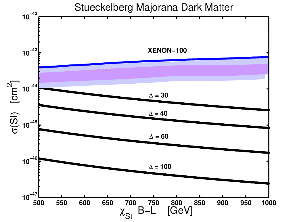
where . In addition, there are terms of size (where are given in [86, 88, 89]). Here terms in that are proportional to are suppressed by a factor of 4 relative to [87]. Terms in also contain and are ultra suppressed by the smallness of the squark mixing angle. For the case when the is relatively close in mass to , up to correction in the light quark masses, there is an enhancement in the SI cross section[87]. Utilizing this effect, for mass splitting of order 30-100 GeV, one easily sees detectable size SI cross sections for squark masses that are in accord with LHC limits (see Fig.(5)). At even smaller mass splittings, the models are constrained by XENON. We have verified using micromegas [90] that the small mass splitting between the LSP and the squarks can lead to cross sections of the size we find. In this case the relic density can be brought in accord with WMAP from co-annihilatons. In particular the squarks in the initial state annihilations play a large role in reducing the relic abundance. There is also mixing that derives from rotating between the chiral fermion in the Stueckelberg multiplet. We consider the optimal case where in the mass diagonal basis, the lighter of the two mass eigenstates is the one which couples via the larger mixing. Thus we have taken the mixing in the gaugino stino sector , and have fixed in Fig.(5). The result of a large scattering cross section does require an LSP above around (500-600) GeV to be consistent with the current limits from the LHC [91, 92, 93, 94, 95].
VI.2 Dirac Dark Matter
Additional matter fields in the form of Dirac fermions (and their supersymmetric counter parts, two chiral scalars) can exist in the sector which have only vectorial couplings to the gauge field and a mass for the Dirac fermions can be generated via terms in the superpotential [37]. As seen already, after mixing of the gauge field with the field , two mass eigenstates and arise in the mass diagonal basis each of which have type couplings with the SM fields. In addition, the interaction of the dark sector Dirac field with the is given by
| (63) |
The interaction vertices with the Dirac particle () with the visible sector quarks and leptons enter through the vector mixings so that
| (64) |
The dark sector Dirac field can constitute dark matter. It is stable and electrically neutral. Since the model we consider has two components of dark matter, the total relic density will be shared by the neutralino and Dirac particles. In the analysis we assume that the dark matter densities for the two components in the galaxy are proportional to their respective relic densities such that sum is the total cold dark matter (CDM) density
| (65) |
The annihilation cross section of into quarks and leptons via the poles is given by
| (66) |
where the poles and couplings enter as
| (67) | |||||
| (68) | |||||
| (69) |
and where , , and for (leptons, quarks). The relevant partial decay widths were given in Table (1) . In addition the can decay into the Dirac sector:
| (70) |
where and . The partial decay width of the is obtained with and in Eq.(70). The relic density can be calculated by integration over the poles. For the technique of integrating over a pole see [97, 98, 99]. The relic density for the 2 components of dark matter can be calculated [37] where for the Dirac component
| (71) |
In Fig. (6) we exhibit a satisfaction of the relic density within the WMAP constraint so that
| (72) |
where the black bands in Fig. (6) show a presumed fraction of the the total relic abundance.


Now, unlike the cases studied previously with the Stueckelberg mass growth, here the dark Dirac fermion does not carry a milli-charge and is electrically neutral. The reason the Dirac fermion is neutral is because there is no mixing of the Stueckelberg gauge field with the hypercharge vector boson. Because of its electrical neutrality and unlike a milli charged particle it cannot be stopped by the atmosphere or by dirt and rock in the Earth before it reaches an underground detector. The effective Lagrangian describing the scattering of a dark Dirac fermion from a quark, in the limit of low momentum transfer, is given by . The corresponding spin independent D-proton cross section is
| (73) |
where and is the reduced mass.
| 200 | 1.9 | 7.5 |
|---|---|---|
| 300 | 3.7 | 1.5 |
| 400 | 1.2 | 4.7 |
| 500 | 4.8 | 1.9 |
Interestingly, for mixing of the size considered in Fig. (1), () and for natural size couplings and one obtains a spin independent cross sections which are of the size
| (74) |
Since , , is essentially independent of . However, compatibility with the WMAP data for the thermal relic density, restricts the ratio . Using this constraint the spin independent cross section for the case is given by
| (75) |
which now has a very strong dependence on the Dirac mass. The numerical size of as a function of the Dirac mass is exhibited in Fig.(5), and the analysis shows that the predicted by the model is accessible in the XENON experiment. In fact for given values of the current limits from XENON100 already put lower limits on the Dirac mass. We can also use the current upper limit on from the XENON100 experiment which gives cm2 for a WIMP mass of 50 GeV, to put a general constraint on so that
| (76) |
We note again that the preceding analysis is very different from the previous Stueckelberg analyses where the
Dirac fermion in the hidden sector develops a milli charge. As already pointed out this arises in models
where one mixes
the Stueckelberg gauge boson with the hypercharge gauge field. In this case the scattering of the Dirac
fermion from a quark will have not only the pole in the t-channel but also a boson pole and
a photon pole as well.
In the present model the and the photon pole are both absent. The Dirac dark matter candidate
is electrically neutral.
As mentioned earlier, for , the relic density will always be satisfied for perturbative size couplings. For but close to the signal will manifest at colliders and the relic density can also be satisfied. However, for the case , while the relic density can be satisfied, the signal becomes suppressed due to the branching ratio into the hidden sector overtaking the branching ratio in the visible sector in the presence of mass and kinetic mixings [100]. In addition, the Breit-Wigner enhancement of the annihilation of Dirac particles in the halo [41] can be operative very close to the pole and the following three possibilities become simultaneous observables:
- 1.
Observation of a very light and narrow vector boson in the dilepton channel at the LHC (see also [5]).
- 2.
- 3.
Relic abundance of dark matter split between a neutralino and dark Dirac (see also [37]) .
- 4.
Observational prospects for the corresponding Dark Dirac component in direct detections experiments such as XENON (analyzed here for the neutral dark Dirac particle via the Stueckelberg mechanism).
Let us add, that just recently, the 730 kg days of the CRESST-II Dark Matter Search was released [102]. Two preferred regions are reported on, and one such region appears close to the CoGeNT preferred region [103]. Very low mass neutralino dark matter with MSSM field content and cross sections of the size needed to explain the CoGeNT are not consistent with the collider constraints [104]. This result has been confirmed by the LHC with its updated constraints on the SUSY Higgs sector [105], wherein large and low mass SUSY Higgs of the size needed to explain the spin-independant scattering are further excluded. The preferred region reported by CRESST-II with heavier dark matter mass may be accommodated for a thermal relic with relic density satisfied via the Z-pole in the MSSM. Such could arise with non-universal gaugino masses at the the high-scale (see [93]) leading to WIMP masses close to 45 GeV. The far boundary of the CRESST-II region terminating close to 55 GeV may also be achieved with relic density satisfied via the Higgs pole (see the analysis of [106]). A dedicated analyses with the new constraints on the SUSY Higgs sector from the LHC [105] would be needed to make a more definitive statement - however the CRESST-II results at these potential dark mater masses do not correspond to reported event rates with CDMS or XENON [51, 50]. The extended model class we discuss can produce spin independent cross sections with larger cross sections than that of the MSSM via the Dirac component of Dark Matter (see Fig.(7)).
VII Discriminating Stueckelberg from Models with Spontaneous Breaking
One may discriminate between the Stueckelberg mass growth for a gauge
boson in the models discussed here and other models where the mass growth for
the gauge boson occurs
by spontaneous breaking. In the above, we have already discussed the mass growth of a gauge
boson by the Stueckelberg mechanism. For the case when the mass growth occurs via spontaneous breaking
there are two possibilities: (i) spontaneous symmetry breaking of occurs violating
R-parity invariance, (ii) spontaneous symmetry breaking of occurs without violating
R-parity invariance. We discuss these two cases below individually.
VII.1 Spontaneous Symmetry Breaking of and R-parity Violation
The simplest example of this is when we consider the superpotential of
Eq.(13). Let us assume that the potential of the field is such that it develops a
VEV. In this case one will have a spontaneous breaking of not only but also of
R-parity as indicated by the term in Eq.(13) after develops a VEV.
In the mass diagonal basis it will lead to other R-parity violating terms, i.e.,
and . Here the LSP is no longer stable and specifically the neutralino cannot
be a dark matter particle. Further, since the neutralino is not stable, the signals of supersymmetry
for this case will be very different at hadron colliders. Specifically if the neutralino decays
inside the detector, there will be no missing energy signatures which are the typical
hallmarks of supersymmetry signatures with R-parity symmetry. Further, for the case when there is
a spontaneous breaking of R-parity symmetry via the VEV growth of the right handed sneutrino, there
will be D term contributions to the slepton squared masses proportional to [7]. Such terms are
absent for the case when the mass growth for the gauge boson occurs preserving R-parity
invariance as discussed below.
VII.2 Models for R-parity Conservation
We further consider now the possibility that symmetry is broken but a residual R-parity symmetry still persists. This is indeed possible following the general line of reasoning of [107] (see also [108]). Thus consider additional fields in the theory such as a vector like multiplet which has the quantum numbers as follows
| (77) |
Let us suppose that one manufactures a potential so that VEV formation for the fields and occurs. In this case will be broken. However, as long as is an even integer R-parity will be preserved. This means that the residual theory will have a R-parity symmetry. Thus, for example, the VEV formation of a scalar field with will violate but preserve R-parity. In the process of the mass mass growth of the gauge boson, one combination of the imaginary parts of and will be absorbed while there would three spin zero fields: 2 CP even and one CP odd (the part orthogonal to the imaginary parts of and which is absorbed) Higgs field. In contrast for the model discussed here, one is left with only two additional scalars, , or , which are both CP even. Specifically there is no additional CP odd Higgs boson for the Stueckelberg models. So this provides a discrimination between the two models.
There are several interesting and distinguishing features between the model and the model. This difference can be seen by comparing Eq.(23) vs Eq.(30). Thus in Eq.(23) one finds that the mass growth of a gauge boson by spontaneous breaking or by the Stueckelberg mechanism would require the gauge boson to be very heavy. Thus for , one will typically have a mass of the gauge boson to be greater than [69, 109]. In contrast, from Eqs.(30) we find that in the model, there are two extra massive gauge bosons beyond what one has in the Standard Model. Thus the heavier one, i.e., the gauge boson, is indeed several TeV in mass. However, the boson we discuss can be much lighter, and can lie in the few hundred GeV range. Thus the observation of a low lying with decay branching ratios characteristic of a gauge boson will be a clear indication of the Stueckelberg model involving mixing of and discussed here.
VIII Conclusion
In this work we have proposed the Stueckelberg mechanism for the mass growth of a gauge boson. It was then shown that under the constraints of charge conservation and the absence of a Fayet-Iliopoulos D term, that R-parity cannot be spontaneously broken in the minimal model of radiative electroweak symmetry breaking. The above is in contrast to models where the mass of the gauge boson is generated by the Higgs mechanism through the VEV formation for the field which breaks R-parity.
A comparison to the case where the symmetry is spontaneously broken but the R-parity symmetry is preserved was also given and its distinguishing features from the Stueckelberg mass growth for the gauge boson are uncovered. Further, we analyzed a Stueckelberg extension of MSSM where a massive boson with interactions can lie in the sub TeV region, i.e, TeV. The observation of a in the sub TeV region with quantum numbers deduced via branching ratios into charged leptons will provide a test of the Stueckelberg extension discussed here.
Other tests of the proposed Stueckelberg models were also discussed. This includes an analysis of the production and decay of the Stueckelberg spin 0 boson which has only loop decays into SM final states via sfermion loops. An interesting decay of the is into was analyzed and shown to have the possibility of observation at the LHC with TeV.
With hidden sector Dirac fermions in the Stueckelberg extension,
two component dark matter manifests, with one component
being either the MSSM neutralino or the Stueckelberg neutralino and the other component being a neutral Dirac
fermion. An analysis of the relic density for the Stueckelberg neutralino and the Stueckelberg neutralino-proton spin independent cross section were also discussed.
An analysis of the
second dark matter component consisting of the Dirac fermion as dark matter was also given and it was shown that
the current XENON100 data already puts constraints on the Dirac fermion mass and mixing angles. The constraints
from the XENON100 data and the LHC data on the couplings of the boson and dark Dirac fermion were shown to
be comparable, both of which limit the mixing of the and dark sector.
Thus the proposed model produces LHC and dark matter signals at mass scales
that are accessible to such experiments and will be tested further as the new data comes in.
Acknowledgments: P.F.P. would like to thank Northeastern University for hospitality in the beginning of this project. The work of D.F. is supported by DOE DE-FG02-95ER40899 and by the Michigan Center for Theoretical Physics. The work of P. F. P. is supported by the James Arthur Fellowship at CCPP-New York University. The work of P.N. is supported in part by NSF grant PHY-0757959 and PHY-0704067. D.F. would like to thank CERN Theory Group for their hospitality while this work was nearing completion.
References
- [1] P. Nath and P. Fileviez Perez, Phys. Rept. 441, 191 (2007).
- [2]
A. H. Chamseddine, R. L. Arnowitt, P. Nath,
Phys. Rev. Lett. 49, 970 (1982);
R. L. Arnowitt and P. Nath,
Phys. Rev. Lett. 69, 725 (1992);
Phys. Lett. B 287, 89 (1992).
For a review see P. Nath, [hep-ph/0307123]. - [3] H. Goldberg, Phys. Rev. Lett. 50, 1419 (1983).
- [4] B. Kors and P. Nath, Phys. Lett. B 586, 366 (2004); JHEP 0412, 005 (2004); JHEP 0507, 069 (2005).
- [5] D. Feldman, Z. Liu and P. Nath, Phys. Rev. Lett. 97, 021801 (2006).
- [6] D. Feldman, Z. Liu and P. Nath, JHEP 0611, 007 (2006).
- [7] P. Fileviez Perez and S. Spinner, Phys. Lett. B 673, 251 (2009).
- [8] V. Barger, P. Fileviez Perez and S. Spinner, Phys. Rev. Lett. 102, 181802 (2009).
- [9] P. Fileviez Perez and S. Spinner, Phys. Rev. D 80, 015004 (2009).
- [10] L. L. Everett, P. Fileviez Perez and S. Spinner, Phys. Rev. D 80, 055007 (2009).
- [11] P. Fileviez Perez and S. Spinner, Phys. Rev. D 83, 035004 (2011).
- [12] P. Fileviez Perez, S. Spinner and M. K. Trenkel, arXiv:1103.5504 [hep-ph].
- [13] S. P. Martin, Phys. Rev. D 46, 2769 (1992).
- [14] S. Khalil and A. Masiero, Phys. Lett. B 665, 374 (2008).
- [15] M. Frank, Phys. Rev. D 63, 034009 (2001).
- [16] C. S. Aulakh and R. N. Mohapatra, Phys. Lett. B 119, 136 (1982).
- [17] L. J. Hall and M. Suzuki, Nucl. Phys. B 231, 419 (1984).
- [18] A. Masiero and J. W. F. Valle, Phys. Lett. B 251, 273 (1990).
- [19] R. N. Mohapatra, Phys. Rev. D 34, 3457 (1986).
- [20] A. Font, L. E. Ibanez and F. Quevedo, Phys. Lett. B 228, 79 (1989).
- [21]
E. Accomando, A. Belyaev, L. Fedeli, S. F. King and C. Shepherd-Themistocleous,
Phys. Rev. D 83, 075012 (2011). - [22] L. Basso, [arXiv:1106.4462 [hep-ph]];G. M. Pruna, arXiv:1106.4691 [hep-ph]; L. Basso, A. Belyaev, S. Moretti, G. M. Pruna and C. H. Shepherd-Themistocleous, PoS ICHEP2010, 381 (2010).
- [23] D. Feldman, B. Kors and P. Nath, Phys. Rev. D 75, 023503 (2007).
- [24] K. Cheung and T. C. Yuan, JHEP 0703, 120 (2007).
- [25] D. Feldman, Z. Liu and P. Nath, Phys. Rev. D 75, 115001 (2007).
- [26]
D. Feldman, Z. Liu, P. Nath,
AIP Conf. Proc. 1078, 116-121 (2009).
AIP Conf. Proc. 939, 50-58 (2007). - [27] M. Pospelov, A. Ritz and M. B. Voloshin, Phys. Lett. B 662, 53 (2008).
- [28] J. L. Feng and J. Kumar, Phys. Rev. Lett. 101, 231301 (2008).
- [29] A. Ibarra, A. Ringwald and C. Weniger, JCAP 0901, 003 (2009).
- [30] Y. Cui, D. E. Morrissey, D. Poland and L. Randall, JHEP 0905, 076 (2009).
- [31] C. Cheung, J. T. Ruderman, L. T. Wang and I. Yavin, Phys. Rev. D 80, 035008 (2009).
- [32] S. Gopalakrishna, S. J. Lee and J. D. Wells, Phys. Lett. B 680, 88 (2009).
- [33] K. Cheung, K. H. Tsao and T. C. Yuan, arXiv:1003.4611 [hep-ph].
- [34] P. Nath, Mod. Phys. Lett. A25, 3003-3016 (2010). [arXiv:0812.0958 [hep-ph]].
- [35] Z. Liu, Nucl. Phys. Proc. Suppl. 200-202, 133 (2010) [arXiv:0910.0061 [hep-ph]].
- [36] For additional works see : D. Feldman, Z. Liu, L. Wang and K. Zurek in Nucl. Phys. Proc. Suppl. 200-202, 185 (2010), Chapter 8 pg. 136 of [arXiv:1001.2693 [hep-ph]].
- [37] D. Feldman, Z. Liu, P. Nath and G. Peim, Phys. Rev. D 81, 095017 (2010).
- [38] D. Feldman, Z. Liu and P. Nath, Phys. Rev. D 79, 063509 (2009).
- [39] N. Arkani-Hamed, D. P. Finkbeiner, T. R. Slatyer and N. Weiner, Phys. Rev. D 79, 015014 (2009).
- [40]
D. Feldman, Z. Liu, P. Nath and B. D. Nelson,
Phys. Rev. D 80, 075001 (2009);
N. Chen, D. Feldman, Z. Liu, P. Nath and G. Peim, Phys. Rev. D 83, 023506 (2011); Phys. Rev. D 83, 035005 (2011). - [41] D. Feldman “Superparticle Signatures: From PAMELA to the LHC,” Nucl. Phys. Proc. Suppl. 200-202, 82 (2010) [arXiv:0908.3727 [hep-ph]].
- [42] A. Arvanitaki, N. Craig, S. Dimopoulos, S. Dubovsky and J. March-Russell, Phys. Rev. D 81, 075018 (2010).
- [43] M. Ahlers, J. Jaeckel, J. Redondo, A. Ringwald, Phys. Rev. D78, 075005 (2008).
- [44] M. Goodsell, J. Jaeckel, J. Redondo, A. Ringwald, JHEP 0911, 027 (2009); J. Jaeckel, A. Ringwald, Ann. Rev. Nucl. Part. Sci. 60, 405-437 (2010).
- [45] M. Williams, C. P. Burgess, A. Maharana and F. Quevedo, arXiv:1103.4556 [hep-ph].
- [46] Y. Mambrini, arXiv:1104.4799 [hep-ph].
- [47] A. E. Nelson and J. Scholtz, arXiv:1105.2812 [hep-ph].
- [48] Y. Mambrini, arXiv:1012.0447 [hep-ph].
- [49] E. Komatsu et al. [WMAP Collaboration], Astrophys. J. Suppl. 192, 18 (2011).
- [50] E. Aprile et al. [XENON100 Collaboration], arXiv:1104.2549 [astro-ph.CO].
- [51] Z. Ahmed et al. [The CDMS-II Collaboration], Science 327, 1619 (2010).
- [52] D. Feldman, Z. Liu and P. Nath, Phys. Rev. D 75, 115001 (2007).
- [53] S. A. Abel, M. D. Goodsell, J. Jaeckel, V. V. Khoze and A. Ringwald, JHEP 0807, 124 (2008).
- [54] Y. Zhang, Chin. Phys. Lett. 26, 081102 (2009); arXiv:1106.0163 [hep-ph]. Y. Zhang and Q. Wang, arXiv:1011.4418 [hep-ph].
- [55] C. Burgess, J. Conlon, L. Hung, C. Kom, A. Maharana and F. Quevedo, JHEP 0807, 073 (2008).
- [56] J. Heeck and W. Rodejohann, arXiv:1109.1508 [hep-ph].
- [57] C. Coriano, M. Guzzi, N. Irges and A. Mariano, Phys. Lett. B 671, 87 (2009); C. Coriano, M. Guzzi, A. Mariano and S. Morelli, Phys. Rev. D 80, 035006 (2009); C. Coriano, M. Guzzi, G. Lazarides and A. Mariano, Phys. Rev. D 82, 065013 (2010).
- [58] P. Anastasopoulos, F. Fucito, A. Lionetto, G. Pradisi, A. Racioppi and Y. S. Stanev, Phys. Rev. D 78, 085014 (2008).
- [59] F. Fucito, A. Lionetto and A. Mammarella, arXiv:1105.4753 [hep-ph]. F. Fucito, A. Lionetto, A. Mammarella and A. Racioppi, Eur. Phys. J. C 69, 455 (2010).
- [60] G. Panotopoulos and P. Tuzon, JHEP 1107, 039 (2011).
- [61] P. G. Camara, L. E. Ibanez and F. Marchesano, arXiv:1106.0060 [hep-th].
- [62] M. J. Dolan, J. Marsano, N. Saulina and S. Schafer-Nameki, arXiv:1102.0290 [hep-th].
- [63] M. Cvetic, J. Halverson and P. Langacker, arXiv:1108.5187 [hep-ph].
- [64] M. Kalb and P. Ramond, Phys. Rev. D 9, 2273 (1974).
- [65] P. Fayet and J. Iliopoulos, Phys. Lett. B 51, 461 (1974).
- [66] S. P. Martin, M. T. Vaughn, Phys. Rev. D50, 2282 (1994). [hep-ph/9311340].
- [67] P. Nath, R. L. Arnowitt, Phys. Rev. D56, 2820-2832 (1997). [hep-ph/9701301].
- [68] M. Ambroso, B. Ovrut, JHEP 0910, 011 (2009); Int. J. Mod. Phys. A 25, 2631 (2010); arXiv:1005.5392 [hep-th].
- [69] M. S. Carena, A. Daleo, B. A. Dobrescu and T. M. P. Tait, Phys. Rev. D 70, 093009 (2004).
- [70] G. W. Bennett et al. [Muon g-2 Collaboration], Phys. Rev. Lett. 92, 161802 (2004).
- [71] V. M. Abazov et al. [D0 Collaboration], Phys. Lett. B 695, 88 (2011) [arXiv:1008.2023 [hep-ex]].
- [72] T. Sjostrand S. Mrenna and P. Z. Skands, JHEP 0605, 026 (2006).
- [73] PGS-4, J. Conway et al. conway/research/software/pgs/pgs4-general.htm
- [74]
[ATLAS Collaboration]
[arXiv:1108.1582 [hep-ex]].
see also:
ATLAS-CONF-2011-083
http://cdsweb.cern.ch/record/1356190/files/ATLAS-CONF-2011-083.pdf - [75] E. Salvioni, G. Villadoro and F. Zwirner, JHEP 0911, 068 (2009).
- [76] M. S. Chanowitz, arXiv:1102.3672 [hep-ph].
- [77] [CMS Collaboration], JHEP 1105, 093 (2011).
- [78] A. Djouadi, Phys. Lett. B 435, 101 (1998).
- [79] M. Spira, Fortsch. Phys. 46, 203 (1998).
- [80] G. F. Giudice, R. Rattazzi and J. D. Wells, Nucl. Phys. B 595, 250 (2001).
- [81] A. De Rujula, J. Lykken, M. Pierini, C. Rogan and M. Spiropulu, Phys. Rev. D 82, 013003 (2010).
- [82] I. Low, J. Lykken and G. Shaughnessy, arXiv:1105.4587 [hep-ph].
- [83] P. J. Fox, D. Tucker-Smith and N. Weiner, JHEP 1106, 127 (2011) [arXiv:1104.5450 [hep-ph]].
- [84] International Europhysics Conference on High Energy Physics (EPS-HEP 2011), Grenoble France, July 2011; The XXV International Symposium on Lepton Photon Interactions at High Energies (Lepton Photon 11); Tata Institute of Fundamental Research, Mumbai, India, August 2011.
- [85] D. Feldman and G. Kane, Perspectives on Supersymmetry II, Kane, G.K., ed. World Sci.Pub. 2010.
- [86] M. Drees and M. Nojiri, Phys. Rev. D 48, 3483 (1993). Phys. Rev. D 47, 4226 (1993).
- [87] J. Hisano, K. Ishiwata and N. Nagata, Phys. Rev. D 82, 115007 (2010).
- [88] U. Chattopadhyay, T. Ibrahim, P. Nath, Phys. Rev. D60, 063505 (1999).
- [89] A. Corsetti, P. Nath, Phys. Rev. D64, 125010 (2001).
- [90] G. Belanger, F. Boudjema, A. Pukhov, A. Semenov, Comput. Phys. Commun. 180, 747-767 (2009).
- [91] [Atlas Collaboration], Phys. Rev. Lett. 106, 131802 (2011); [CMS Collaboration], Phys. Lett. B 698, 196 (2011) ATLAS Collaboration], arXiv:1103.4344 [hep-ex]. arXiv:1109.2352
- [92]
[ATLAS Collaboration]
ATLAS-CONF-2011-086
http://cdsweb.cern.ch/record/1356194/files/ATLAS-CONF-2011-086.pdf - [93] S. Akula, D. Feldman, Z. Liu, P. Nath and G. Peim, arXiv:1103.5061; arXiv:1107.3535.
- [94] S. Akula, N. Chen, D. Feldman, M. Liu, Z. Liu, P. Nath and G. Peim, Phys. Lett. B 699, 377 (2011).
- [95] O. Buchmueller et al., arXiv:1106.2529 [hep-ph].
- [96] C. Boehm, A. Djouadi and M. Drees, Phys. Rev. D 62, 035012 (2000); For a review see Y. Santoso, and references therein; Nucl. Phys. Proc. Suppl. 124, 166 (2003).
- [97] P. Nath, R. L. Arnowitt, Phys. Rev. Lett. 70, 3696-3699 (1993).
- [98] K. Griest, D. Seckel, Phys. Rev. D43, 3191-3203 (1991).
- [99] P. Gondolo, G. Gelmini, Nucl. Phys. B360, 145-179 (1991).
- [100] D. Feldman, Z. Liu and P. Nath, Phys. Rev. D 75, 115001 (2007); E. J. Chun, J. C. Park and S. Scopel, JHEP 1102, 100 (2011); P. Gondolo, P. Ko and Y. Omura, arXiv:1106.0885 [hep-ph].
- [101] O. Adriani et al. [PAMELA Collaboration], Nature 458, 607 (2009) [arXiv:0810.4995 [astro-ph]]; 2011 Fermi Symposium: http://fermi.gsfc.nasa.gov/science/symposium/2011/
- [102] G. Angloher et al., arXiv:1109.0702 [astro-ph.CO].
- [103] C. E. Aalseth et al. [CoGeNT collaboration], Phys. Rev. Lett. 106, 131301 (2011).
- [104] D. Feldman, Z. Liu and P. Nath, Phys. Rev. D 81, 117701 (2010) [arXiv:1003.0437 [hep-ph]]. E. Kuflik, A. Pierce and K. M. Zurek, Phys. Rev. D 81, 111701 (2010) [arXiv:1003.0682 [hep-ph]]. D. A. Vasquez, G. Belanger, C. Boehm, A. Pukhov and J. Silk, Phys. Rev. D 82, 115027 (2010) [arXiv:1009.4380 [hep-ph]]. J. Cao, K. i. Hikasa, W. Wang and J. M. Yang, arXiv:1104.1754 [hep-ph]. D. T. Cumberbatch, D. E. Lopez-Fogliani, L. Roszkowski, R. R. de Austri and Y. L. Tsai, arXiv:1107.1604 [astro-ph.CO].
- [105] M. Vazques Acosta, on behalf of the ATLAS and CMS Collaborations, SUSY 2011, Fermilab.
- [106] D. Feldman, K. Freese, P. Nath, B. D. Nelson and G. Peim, Phys. Rev. D 84, 015007 (2011) [arXiv:1102.2548 [hep-ph]].
- [107] L. M. Krauss and F. Wilczek, Phys. Rev. Lett. 62, 1221 (1989).
- [108] S. P. Martin, Phys. Rev. D 54, 2340 (1996).
- [109] G. Cacciapaglia, C. Csaki, G. Marandella and A. Strumia, Phys. Rev. D 74, 033011 (2006).