Kirkwood gaps and diffusion along mean motion resonances
in the restricted planar three-body problem
Abstract
We study the dynamics of the restricted planar three-body problem near mean motion resonances, i.e. a resonance involving the Keplerian periods of the two lighter bodies revolving around the most massive one. This problem is often used to model Sun–Jupiter–asteroid systems. For the primaries (Sun and Jupiter), we pick a realistic mass ratio and a small eccentricity . The main result is a construction of a variety of non local diffusing orbits which show a drastic change of the osculating (instant) eccentricity of the asteroid, while the osculating semi major axis is kept almost constant. The proof relies on the careful analysis of the circular problem, which has a hyperbolic structure, but for which diffusion is prevented by KAM tori. In the proof we verify certain non-degeneracy conditions numerically.
Based on the work of Treschev, it is natural to conjecture that the time of diffusion for this problem is . We expect our instability mechanism to apply to realistic values of and we give heuristic arguments in its favor. If so, the applicability of Nekhoroshev theory to the three-body problem as well as the long time stability become questionable.
It is well known that, in the Asteroid Belt, located between the orbits of Mars and Jupiter, the distribution of asteroids has the so-called Kirkwood gaps exactly at mean motion resonances of low order. Our mechanism gives a possible explanation of their existence. To relate the existence of Kirkwood gaps with Arnol’d diffusion, we also state a conjecture on its existence for a typical -perturbation of the product of the pendulum and the rotator. Namely, we predict that a positive conditional measure of initial conditions concentrated in the main resonance exhibits Arnol’d diffusion on time scales .
1 Introduction and main results
1.1 The problem of the stability of gravitating bodies
The stability of the Solar System is a longstanding problem. Over the centuries, mathematicians and astronomers have spent an inordinate amount of energy proving stronger and stronger stability theorems for dynamical systems closely related to the Solar System, generally within the frame of the Newtonian -body problem:
| (1) |
and its planetary subproblem, where the mass (modelling the Sun) is much larger than the other masses .
A famous theorem of Lagrange entails that the observed variations in the motion of Jupiter and Saturn come from resonant terms of large amplitude and long period, but with zero average (see [Las06] and references therein, or [AKN88, Example 6.16]). Yet it is a mistake, which Laplace made, to infer the topological stability of the planetary system, since the theorem deals only with an approximation of the first order with respect to the masses, eccentricities and inclinations of the planets [Lap89, p. 296]. Another key result is Arnol’d’s theorem, which proves the existence of a set of positive Lebesgue measure filled by invariant tori in planetary systems, provided that the masses of the planets are small [Arn63, Féj04]. However, in the phase space the gaps left by the invariant tori leave room for instability.
It was a big surprise when the numerical computations of Sussman, Wisdom and Laskar showed that over the life span of the Sun, or even over a few million years, collisions and ejections of inner planets are probable (due to the exponential divergence of solutions, only a probabilistic result seems within the reach of numerical experiments); see for example [SW92, Las94], or [Las10] for a recent account. Our Solar System, as well as newly discovered extra-solar systems, are now widely believed to be unstable, and the general conjecture about the -body problem is quite the opposite of what it used to be:
Conjecture 1.1 (Global instability of the -body problem).
In restriction to any energy level of the -body problem, the non-wandering set is nowhere dense. (One can reparameterize orbits to have a complete flow, despite collisions.)
According to Herman [Her98], this is the oldest open problem in dynamical systems (see also [Kol57]). This conjecture would imply that bounded orbits form a nowhere dense set and that no topological stability whatsoever holds, in a very strong sense. It is largely confirmed by numerical experiments. In our Solar System, Laskar for instance has shown that collisions between Mars and Venus could occur within a few billion years. The coexistence of a nowhere dense set of positive measure of bounded quasi-periodic motions with an open and dense set of initial conditions with unbounded orbits is a remarkable conjecture.
Currently the above conjecture is largely out of reach. A more modest but still very challenging goal, also stated in [Her98], is a local version of the conjecture:
Conjecture 1.2 (Instability of the planetary problem).
If the masses of the planets are small enough, the wandering set accumulates on the set of circular, coplanar, Keplerian motions.
There have been some prior attempts to prove such a conjecture. For instance, Moeckel discovered an instability mechanism in a special configuration of the -body problem [Moe96]. His proof of diffusion was limited by the so-called big gaps problem between hyperbolic invariant tori; this problem was later solved in this setting by Zheng [Zhe10]. A somewhat opposite strategy was developed by Bolotin and McKay, using the Poincaré orbits of the second species to show the existence of symbolic dynamics in the three-body problem, hence of chaotic orbits, but considering far from integrable, non-planetary conditions; see for example [Bol06]. Also, Delshams, Gidea and Roldán have shown an instability mechanism in the spatial restricted three-body problem, but only locally around the equilibrium point (see [DGR11]).
In this paper we prove the existence of large instabilities in a realistic planetary system and describe the associated instability mechanism. We thus provide a step towards the proof of Conjecture 1.2.
In his famous paper [Arn64], Arnol’d says: ‘‘In contradistinction with stability, instability11 1 In the translation the word “nonstability” is used, which seems to refer to instability. is itself stable. I believe that the mechanism of “transition chain” which guarantees that instability in our example is also applicable to the general case (for example, to the problem of three bodies)”. In this paper we exhibit a regime of realistic motions of a three body problem where “transition chains” do occur and lead to Arnol’d’s mechanism of instability. Such instabilities occur near mean motion resonances, defined below. To the best of our knowledge, this is the first regime of motions of the problem of three bodies naturally modelling a region in the Solar system, where nonlocal transition chains are established22 2 “Nonlocal” means that motions on the boundary tori in this chain differ significantly, uniformly with respect to the small parameter. In our case, the eccentricity of orbits of the massless planet (asteroid) varies by , uniformly with respect to small values of the eccentricity of the primaries, while the semi major axis stays nearly constant. See Section 1.3 for more details.. Previous results showing transition chains of tori in the problem of three bodies naturally modelling a region in the Solar system are confined to small neighborhoods of the Lagrangian Equilibrium points [CZ11, DGR11], and therefore, are local in the Configuration and Phase space.
The instability mechanism shown in this paper is related to a generalized version of Mather’s acceleration problem [Mat96, BT99, DdlLS00, GT08, Kal03, Pif06]. Some parts of the proof rely on numerical computations, but our strategy allows us to keep these computations simple and convincing.
We consider the planetary problem (1) with one planet mass (say, ) larger than the others: . The equations of motion of the lighter objects () can advantageously be written as
| (2) |
Letting the masses tend to for , we obtain a collection of independent restricted problems:
| (3) |
where the massless bodies are influenced by, without themselves influencing, the primaries of masses and .
For , this model is often used to approximate the dynamics of Sun-Jupiter-asteroid or other Sun-planet-object problems, and it is the simplest one conjectured to have a wide range of instabilities.
1.2 An example of relevance in astronomy
1.2.1 The asteroid belt
One place in the Solar system where the dynamics is well approximated by the restricted three-body problem is the asteroid belt. The asteroid belt is located between the orbits of Mars and Jupiter and consists of 1.7 million objects ranging from asteroids of kilometers to dust particles. Since the mass of Jupiter is approximately masses of Mars, away from close encounters with Mars, one can neglect the influence of Mars on the asteroids and focus on the influence of Jupiter. We also omit interactions with the second biggest planet in the Solar System, namely Saturn, which actually is not so small. Indeed, its mass is about a third of the mass of Jupiter and its semi major axis is about times the semi major axis of Jupiter. This implies that the strength of interaction with Saturn is around of the strength of interaction with Jupiter. However, instabilities discussed in this paper are fairly robust and we believe that they are not destroyed by the interaction with Saturn (or other celestial bodies), which to some degree averages out.
With these assumptions one can model the motion of the objects in the asteroid belt by the restricted problem. Denote by the mass ratio, where is the mass of the Sun and is the mass of Jupiter. For (namely, neglecting the influence of Jupiter), bounded orbits of the asteroid are ellipses. Up to orientation, the ellipses are characterized by their semi major axis and eccentricity .
The aforementioned theorem of Lagrange asserts that, for small , the semi major axis of an asteroid satisfies for all . For very small the time of stability was greatly improved by Niederman [Nie96] using Nekhoroshev theory; see the discussion in the next section. Nevertheless, if one looks at the asteroid distribution in terms of their semi major axis, one encounters several gaps, the so-called Kirkwood gaps. It is believed that the existence of these gaps is due to instability mechanisms.
1.2.2 Kirkwood gaps and Wisdom’s ejection mechanism
Mean motion resonances occur when the ratio between the period of Jupiter and the period of the asteroid is rational. In particular, the Kirkwood gaps correspond to the ratios and .

In this section we present a heuristic explanation of the reason why these gaps exist.
It is conjectured and confirmed by numerical data [Wis82] that the eccentricities of asteroids appropriately placed in the Kirkwood gaps change by a magnitude of order one. Notice that in the real data, the eccentricities of most asteroids in the asteroid belt are between and ; see for example http://en.wikipedia.org/wiki/File:Mainbeltevsa.png.

As the eccentricity of the asteroid grows while its semi major axis is nearly constant, its perihelion gets closer and closer to the origin, namely at the distance , where and are the semi major axis and eccentricity of the asteroid respectively (see Figure 2, where the inner circle is the orbit of Mars). In particular, a close encounter with Mars becomes increasingly probable. Eventually Mars and the asteroid come close to each other, and the asteroid most probably gets ejected from the asteroid belt.
A surprising fact is that the change of eccentricity of the asteroid is only possible due to the ellipticity of the motion of Jupiter, due to the following count of dimensions. For circular motions of Jupiter the problem reduces to two degrees of freedom (see Section 1.8) and plausibly there are invariant -dimensional tori separating the three dimensional energy surfaces; see for example [GDF+89, Féj02b, CC07]. If the eccentricity of Jupiter is not zero, the system has two and a half degrees of freedom and then KAM tori do not prevent drastic changes in the eccentricity.
Heuristically, the conclusion is that, if the eccentricity of the asteroid changes by a magnitude of order one in the Sun-Jupiter-asteroid restricted problem, then the asteroid might come into zones where the restricted problem does not describe the dynamics appropriately, due to the influence of Mars.
The main result of this paper is that for certain mean motion resonances there are unstable motions which lead to significant changes in the eccentricity. We only present results for two particular resonances ( and ), because the proof relies on numerical computations. The resonance corresponds to one of most noticeable Kirkwood gaps. We are confident that our mechanism of instability applies to other resonances, and thus to the other Kirkwood gaps, as long as the orbits of the unperturbed problem stay away from collisions. Thus, the instability mechanism showed in this paper gives insight into the existence of the Kirkwood gaps.
Another instability mechanism, using the adiabatic invariant theory, can be seen in [NS04] where a heuristic explanation is given. Let where is mass ratio and is eccentricity of Jupiter. They study the case when is relatively small: . In reality it is close to . In contrast, we study the case of large .
1.2.3 Capture in resonance of other objects
Many known light objects in the Solar System display a mean motion resonance of low order with Jupiter or some other planet. Some of them are: Trojan satellites, which librate around one of the two Lagrangian points of a planet, hence in resonance with the planet; Uranus, which is close to the resonance with Jupiter, thus giving an example of an “outer” restricted problem that is close in phase space to the solutions we are studying; or the Kuiper Belt beyond Neptune, whose objects, behaving in the exact opposite manner to those of the asteroid belt, seem to concentrate close to mean motion resonances (in particular, the Keplerian ellipse of the dwarf planet Pluto notoriously meets the ellipse of Neptune). The current existence of these resonant objects, and thus their relative stability, seemingly contradicts the above mechanism. This calls at least for a short explanation, although there are many effects at work.
The main point is that an elliptic stability zone lies in the eye of a resonance, where some kind of long term stability prevails. Besides, the geometry of the system often prevents the ejection mechanism described in Section 1.2.2, because there is no such body as Mars to propel the asteroid through a close encounter. In many cases, the mean motion resonance itself precludes collisions with the main planet, for example the Trojan asteroids with respect to Jupiter, or Pluto with respect to Neptune; for a discussion of this effect in the asteroid belt, see [Rob05].
The complete picture certainly includes secular resonances, close encounters between asteroids, as well as more complicated kinds of resonance involving more bodies (for example the second Kirkwood gap, where a four-body problem resonance seems to play a crucial role). We refer to [Mor02, Rob05] for further astronomical details.
1.3 Main results
Let us consider the three-body problem and assume that the massless body moves in the same plane as the two primaries. We normalize the total mass to one, and we call the three bodies the Sun (mass ), Jupiter (mass with ) and the asteroid (zero mass). If the energy of the primaries is negative, their orbits describe two ellipses with the same eccentricity, say . For convenience, we denote by the normalized position of the primaries (or “fictitious body”), so that the Sun and Jupiter have respective positions and . The Hamiltonian of the asteroid is
| (4) |
where . Without loss of generality one can assume that has semi major axis equal to 1 and period . For this system has two and a half degrees of freedom.
When , the primaries describe uniform circular motions aroung their center of mass. (This system is called the restricted planar circular three-body problem). Thus, in a frame rotating with the primaries, the system becomes autonomous and hence has only 2 degrees of freedom. Its energy in the rotating frame is a first integral, called the Jacobi integral33 3 Celestial mechanics’s works often prefer to use the Jacobi constant , given by .. It is defined by
| (5) |
The aforementioned KAM theory applies to both the circular and the elliptic problem [Arn63, SM95] and asserts that if the mass of Jupiter is small enough, there is a set of initial conditions of positive Lebesgue measure leading to quasiperiodic motions, in the neighborhood of circular motions of the asteroid.
If Jupiter has a circular motion, since the system has only 2 degrees of freedom, KAM invariant tori are 2-dimensional and separate the 3-dimensional energy surfaces. But in the elliptic problem, 3-dimensional KAM tori do not prevent orbits from wandering on a 5-dimensional phase space. In this paper we prove the existence of a wide enough set of wandering orbits in the elliptic planar restricted three-body problem.
Let us write the Hamiltonian (4) as
with
The Keplerian part allows us to associate elliptical elements to every point of the phase space of negative energy . We are interested in the drift of the eccentricity under the flow of . (The reader will easily distinguish this notation from other meanings of ).
We will see later that uniformly, away from collisions. Notice that there is a competition between the integrability of and the non-integrability of , which allows for wandering. In this work we consider a realistic value of the mass ratio, .
Notation 1.3.
In what follows, we abbreviate the restricted planar circular three-body problem to the circular problem, and the restricted planar elliptic three-body problem to the elliptic problem.
Here is the main result of this paper.
Main Result (resonance ). Consider the elliptic problem with mass ratio and eccentricity of Jupiter . Assume it is in general position44 4 Later we state three Ansätze that formalize the non-degeneracy conditions we need.. Then, for small enough, there exists a time and a trajectory whose eccentricity satisfies that
while

We will make this result more precise in Section 1.8, Theorem 1, after providing some appropriate definitions. We stress that the instabilities discussed in the Main Result are non-local neither in the action space nor in the configuration space. This is the first result showing nonlocal instabilities in the planetary three body problem.
In [GK10b, GK10a, GK11] it is shown that in the circular problem with realistic mass ratio there exists an unbounded Birkhoff region of instability for eccentricies larger than and Jacobi integral . This allows them to prove a variety of unstable motions, including oscillatory motions and all types of final motions of Chazy.
The analogous result for the resonance is as follows.
Main Result (resonance ). Consider the elliptic problem with mass ratio and eccentricity of Jupiter . Assume it is in general position. Then, for small enough, there exists a time and a trajectory whose eccentricity satisfies that
while
Thus we claim the existence of orbits of the asteroid whose change in eccentricity is above . In Appendix D, we state two conjectures about the stochastic behavior of orbits near a resonance: one is for Arnol’d’s example and another one is for our elliptic problem. These conjectures are based on numerical experiments; see for example [Chi79, SUZ88, Wis82]. We also provide some heuristic arguments using the dynamical structures explored in this paper. Loosely speaking, we claim that near a resonance there is polynomial instability for a positive measure set of initial conditions on the time scale .
Most of the paper is devoted to the resonance . But the proof seems robust with respect to the precise resonance considered. In appendix C, we show how to modify the proof of the main result to deal with the resonance , whose importance in explaining the Kirkwood gaps is emphasized in the introduction.
We believe that our mechanism applies to a substantially larger interval of eccentricities, but proving this requires more sophisticated numerics; see Remark A.4.
1.4 Refinements and comments
1.4.1 Smallness of the eccentricity of Jupiter
When Jupiter describes a circular motion, the Jacobi integral is an integral of motion and then KAM theory prevents global instabilities. We consider the eccentricity as a small parameter so that we can compare the dynamics of the elliptic problem with the dynamics of the circular one.
The difference between the elliptic and circular Hamiltonians is . The analysis of the difference, performed in Section 3.2, shows that this difference can be reduced to (or even smaller) using averaging. This makes us believe that does not need to be infinitesimally small for our mechanism to work. Even the realistic value is not out of question. However, having a realistic becomes mostly a matter of numerical experiment, not of mathematical proof —the limit and the interest of perturbation theory is to describe dynamical behavior in terms of asymptotic models. See Appendix D.2 for more details.
1.4.2 On infinitesimally small masses
In the Main Result, we do not know what happens asymptotically if we let , since our estimates worsen. Indeed, one of the crucial steps of the proof is to study the transversality of certain invariant manifolds (see Section 1.6) and this transversality becomes exponentially small with respect to as . On the other hand, the Main Result holds for realistic values of , which is out of reach of many qualitative results of perturbation theory where parameters are conveniently assumed to be as small as needed. See Appendix D for more details.
1.4.3 Speed of diffusion
In Appendix D we discuss the relation of our problem with a priori unstable systems and Mather’s accelerating problem. We conjecture that, for the orbits constructed in this paper, the diffusion time can be chosen to be
| (6) |
Time estimates in the a priori unstable setting can be found in [BB02, BBB03, Tre04, GdlL06].
De la Llave [dlL04], Gelfreich-Turaev [GT08], and Piftankin [Pif06], using Treschev’s techniques of separatrix maps (see for instance [PT07]), proved linear diffusion for Mather’s acceleration problem. Using these techniques, a smart choice of diffusing orbits might lead to even faster diffusion in our problem, in times of the order ; see Appendix D for more details55 5 This does not seem crucial, since the real value is not smaller than ..
An analytic proof of this conjecture might require restrictive conditions between and . However, for realistic values of and or smaller, that is and , we expect that the speed of our mechanism of diffusion also obeys the above heuristic formula.
On the other hand, the above formula probably does not hold in the neighborhood of circular motions of the masless body, which might be much more stable than more eccentric motions. This could explain the fact that Uranus, whose eccentricity of 0.04 is significantly smaller than most asteriods from the asteriod belt, and which is roughly in -resonance with Jupiter (its period is 7.11 times larger than that of Jupiter) has not been expelled yet; see also Section 1.2.3. However, a deeper analysis would require to compare the distances of the various celestial bodies to the mean motion resonance, as well as the splitting of their invariant manifolds.
1.4.4 On Nekhoroshev’s stability
Consider an analytic nearly integrable system of the form with and in the unit ball . Suppose is convex (or even suppose the weaker condition that is steep).66 6 Recall that is called steep if for any affine subspace of the restriction has only isolated critical points. Then a famous result of Nekhoroshev states that for some independent of we have
See for instance [Nie96] for the history and precise references and [Xue10] for the estimate on the involved constant .
Niederman [Nie96] applied Nekhoroshev theory to the planetary -body problem. He showed that the semi major axis obeys the above estimate for exponentially long time, , with being the smallness of the planetary masses. However, the constant along with other constants involved in the proof are not optimal. Specifically, needs to be as small as to have stability time comparable to the age of the Solar system. Moreover, the stability of semi major axis does not imply the stability of the eccentricity, which we conjecture has substantial deviations in polynomially long time.
Notice that our results along the predictions of Treschev’s (see Appendix D) state the possibility of polynomial instability for eccentricities for the elliptic problem.
With , there was a hope to apply this result to the long time stability of e.g. the Sun-Jupiter-Saturn system; see [GG85]). However, (6) indicates absence of even -stability. Indeed, the unperturbed Hamiltonian of the three body problem is neither convex, nor steep. This turns out to be not just a technical problem but a true obstruction to exponentially long time stability, since Nekhoroshev’s theory does not apply to this kind of systems. See Appendix D for more details.
1.5 Mechanism of instability
The Main Result gives an example of large instability for this mechanical system. It can be interpreted as an example of Arnol’d diffusion; see [Arn64]. Nevertheless, Arnol’d diffusion usually refers to nearly integrable systems, whereas Hamiltonian (4) cannot be considered so close to integrable since . The mechanism of diffusion used in this paper is similar to the so-called Mather’s accelerating problem ([Mat96, BT99, DdlLS00, GT08, Kal03, Pif06]). This analogy is explained in Section 2.3.
Arguably, the main source of instabilities are resonances. One of the most natural kind of resonances in the three-body problem is mean motion orbital resonances77 7 The mean motions are the frequencies of the Keplerian revolution of Jupiter and the asteroid around the Sun: in our case the asteroid makes one full revolution while Jupiter makes seven revolutions.. Along such a resonance, Jupiter and the asteroid will regularly be in the same relative position. Over a long time interval, Jupiter’s perturbative effect could thus pile up and (despite its small amplitude due to the small mass of Jupiter) could modify the eccentricity of the asteroid, instead of averaging out.
According to Kepler’s third Law, this resonance takes place when is close to a rational, where is the semi major axis of the instant ellipse of the asteroid. In our case we consider close to 7 in Section 1.8 and close to in appendix C. Nevertheless, we expect that the same mechanism takes place for a large number of mean motion orbital resonances.
The semi major axis and the eccentricity describe completely an instant ellipse of the asteroid (up to orientation). Thus, geometrically the Main Results say that the asteroid evolves from a Keplerian ellipse of eccentricity to one of eccentricity (for the resonance ) and from to (for the resonance ), while keeping its semi major axis almost constant; see Figure 2. In Figure 3 we consider the plane , which describes the ellipse of the asteroid. The diffusing orbits given by the Main Results correspond to nearly horizontal lines.

A qualitative description of such a diffusing orbit is given at the end of section 4.
1.6 Sketch of the proof
Our overall strategy is to:
- (A)
Carefully study the structure of the restricted three-body problem along a chosen resonance.
- (B)
Show that, generically within the class of problems sharing the same structure, global instabilities exist. One could say that this step is similar, in spirit, to “abstract” proofs of existence of instabilities for generic perturbations of a priori chaotic systems such as in Mather’s accelerating problem.
- (C)
Check numerically that the generic conditions (which we call Anzätze) are satisfied in our case.
Step (B) is the core of the paper and we now give more details about it.
For the elliptic problem, the diffusing orbit that we are looking for lies in a neighborhood of a (-dimensional) normally hyperbolic invariant cylinder and its local invariant manifolds, which exist near our mean motion resonance. The vertical component of the cylinder can be parameterized by the eccentricity of the asteroid and the horizontal components by its mean longitude and time.
If the stable and unstable invariant manifolds of intersect transversally, the elliptic problem induces two different dynamics on the cylinder (see Sections 3.4 and 3.5): the inner and the outer dynamics. The inner dynamics is simply the restriction of the Newtonian flow to . The outer dynamics is obtained by a limiting process: it is observed asymptotically by starting very close to the cylinder and its unstable manifold, traveling all the way to a homoclinic intersection, and coming back close to the cylinder along its stable manifold; see Definition 2.3.
Since the system has different homoclinic orbits to the cylinder, one can define different outer dynamics. In our diffusing mechanism we use two different outer maps. The reason is that each of the outer maps fails to be defined in the whole cylinder, and so we need to combine the two of them to achieve diffusion; see Section 2.
The proof consists in the following five steps:
- 1.
Construct a smooth family of hyperbolic periodic orbits for the circular problem with varying Jacobi integral (Ansatz 1).
- 2.
- 3.
- 4.
- 5.
Construct diffusing orbits by shadowing such a polyorbit (Lemma 4.4).
This program faces difficulties at each step, as explained next.
1.6.1 Existence of a family of hyperbolic periodic orbits of the circular problem
This part is mainly numerical. Using averaging and the symmetry of the problem we guess a location of periodic orbits of a certain properly chosen Poincare map of the circular problem. Then for an interval of Jacobi integral and each we compute them numerically and verify that they are hyperbolic. For infinitesimally small hyperbolicity follows from averaging.
1.6.2 Existence of a normally hyperbolic invariant cylinder
The first difficulty comes from the proper degeneracy of the Newtonian potential: at the limit (no Jupiter), the asteroid has a one-frequency, Keplerian motion, whereas symplectic geometry allows for a three-frequency motion (as with any potential other than the Newtonian potential and the elastic potential ). Due to this degeneracy, switching to (even with ) is a singular perturbation.
1.6.3 Transversality of the stable and unstable invariant manifolds
Establishing the transversality of the invariant manifolds of , is a delicate problem, even for . Asymptotically when , the difference (splitting angle) between the invariant manifolds becomes exponentially small with respect to , that is of order for some constant . Despite inordinate efforts of specialists, all known techniques fail to estimate this splitting, because the relevant Poincaré-Melnikov integral is not algebraic. Note that this step is significantly simpler when one studies generic systems.
At the expense of creating other difficulties, setting avoids this splitting problem, since for this value of the parameter we see that the splitting of separatrices is not extremely small and can be detected by means of a computer. Besides, is a realistic value of the mass ratio for the Sun-Jupiter model. Since the splitting of the separatrices varies smoothly with respect to the eccentricity of the primaries, it suffices to estimate the splitting for , that is in the circular problem. This is a key point for the numerical computation, which thus remains relatively simple. On the other hand, in the next two steps it is crucial to have , otherwise the KAM tori separates the Jacobi integral energy levels.
Moreover, recall that the cylinder has two branches of both stable and unstable invariant manifolds (both originated by a family of periodic orbits of the circular problem, see Figures 17, 18 for and Figures 26, 28 for ). In certain regions, the intersection between one of the branches of the stable and unstable invariant manifolds is tangential, which prevents us from defining the outer map. Nevertheless, then we check that the other two branches intersect transversally and we define a different outer map. Thus, we combine the two outer maps depending on which branches of the invariant manifolds intersect transversally.
1.6.4 Asymptotic formulas for the outer and inner maps
Using classical perturbation theory and the specific properties of the underlying system, we reduce the inner and (the two different) outer dynamics to three -dimensional symplectic smooth maps of the form
| (7) |
and
| (8) |
where are conjugate variables which parameterize a connected component of the 3-dimensional normally hyperbolic invariant cylinder intersected with a transversal Poincaré section, and are smooth functions. The superindexes and stand for the forward and backward heteroclinic orbits that are used to define the outer maps. The choice of this notation will be clear in Section 2. Note that these maps are real and thus and are complex conjugate to and respectively.
1.6.5 Non-degeneracy implies the existence of diffusing orbits
As shown in Section 4, the existence of diffusing orbits is established provided that the smooth functions
| (9) |
do not vanish on the set where the corresponding outer map is defined. Since and are complex conjugate, as well as and , we do not need to consider the complex conjugate . We check numerically that in their domain of definition. The conditions imply the absence of common invariant curves for the inner and outer maps. This reduces the proof of the Main Result to shadowing, which therefore leads to the existence of diffusing orbits.
It turns out that, in this problem, no large gaps appear. This fact is not surprising since the elliptic problem has three time scales.
Finally, notice that the complex functions can be regarded as a 2-dimensional real-valued function depending smoothly on . If the dependence on is non-trivial, a complex valued function does not vanish at any point of its domain of definition except for a finite number of values .
1.7 Nature of numerics
In this section we outline which parts of the mechanism are based on numerics.
- •
On each -dimensional energy surface the circular problem has a well-defined Poincaré map of a -dimensional cylinder for a range of energies . For each in some interval we establish the existence of a saddle periodic orbit such that .
- •
We show that for all there are two intersections of and . Each intersection is transversal for almost all values of , but it becomes tangent at an exceptional (discrete) set of values of . Nevertheless, we check that at least one of the two intersections is transversal for each ; see Figure 15.
- •
Each transversal intersection gives rise to a homoclinic orbit, denoted . For each we compute several Melnikov integrals of certain quantities related to along and . Out of these integrals we compute the leading terms of the dynamics of the elliptic problem and verify a necessary condition for diffusion.
1.8 Main theorem for the resonance
The model of the Sun, Jupiter and a massless asteroid in Cartesian coordinates is given by the Hamiltonian (4). First, let us consider the case , that is, we consider Jupiter with zero mass. In this case, Jupiter and the asteroid do not influence each other and thus the system reduces to two uncoupled 2-body problems (Sun-Jupiter and Sun-asteroid) which are integrable.
Let us introduce the so-called Delaunay variables, denoted by , which are angle-action coordinates of the Sun-asteroid system. The variable is the mean anomaly, is the square root of the semi major axis, is the argument of the perihelion and is the angular momentum. Delaunay variables are obtained from Cartesian variables via the following symplectic transformation (see [AKN88] for more details and background, or [Féj13, Appendix] for a straightforward definition). First define polar coordinates for the position:
Then, the actions of the Delaunay coordinates are defined by
| (10) |
(recall that for these definitions). Using these actions, the eccentricity of the asteroid is expressed as
| (11) |
To define the angles and , let be the true anomaly, so that
| (12) |
Then, from one can obtain the eccentric anomaly using
| (13) |
From the eccentric anomaly, the mean anomaly is given by Kepler’s equation
| (14) |
We apply the Delaunay change of coordinates given above to the elliptic problem; see Appendix B.1. In Delaunay coordinates, the Hamiltonian (4) can be split into the Keplerian part , the circular part of the perturbing function , and the remainder which vanishes when :
| (15) |
For , the circular problem only depends on . To simplify the comparison with the circular problem, we consider rotating Delaunay coordinates, in which is autonomous. Define the new angle (the argument of the pericenter, measured in the rotating frame) and a new variable conjugate to time . Then we have
| (16) |
In these new variables, the difference in the number of degrees of freedom of the elliptic and circular problems becomes more apparent. When the system is autonomous and then is constant, which corresponds to the conservation of the Jacobi integral (5). Therefore, the circular problem reduces to 2 degrees of freedom. Moreover, it will later be crucial to view the circular problem as an approximation of the elliptic one, in order to reduce the (possibly impracticable) numerical computations needed by a direct approach to the corresponding lower dimensional, and thus simpler, computations of the circular problem.
Recall that, in this section, we consider the mean motion orbital resonance between Jupiter and the asteroid, that is, the period of the asteroid is approximately seven times the period of Jupiter. In rotating Delaunay variables, this corresponds to
| (17) |
A nearby resonance is but we stick to the previous one.
The resonance takes place when . We study the dynamics in a large neighborhood of this resonance and we show that one can drift along it. Namely, we find trajectories that keep close to while the -component changes noticeably. Using (11), we see that also changes by order one. In this setting, the Main Result can be rephrased as follows.
Theorem 1.
Ansätze 1 (Section 2), 2 (Section 2) and 3 (Section 4) are hypotheses which, broadly speaking, assert that the Hamiltonian (16) is in general position in some domain of the phase space; see also Section 1.7. They are backed up by the numerics in the appendices.
By definition the Hamiltonian (16) is autonomous and thus preserved. Hence, we will restrict ourselves to a level of energy which, without loss of generality, can be taken as . Therefore, since , the drift in is equivalent to the drift in for orbits satisfying .
The proof of Theorem 1 is structured as follows.
- 1.
Ansatz 1 says that for an interval of Jacobi energies the circular problem has a smooth family of hyperbolic periodic orbits , whose stable and unstable manifolds intersect transversally for each .
- 2.
Ansatz 2 asserts that the period of these periodic orbits changes monotonically with respect to the Jacobi integral.
- 3.
Ansatz 3 asserts that Melnikov functions associated with symmetric homolinic orbits created by the above periodic orbits are in general position.
Ansatz 1 implies the existence of a normally hyperbolic invariant cylinder (Corollary 2.1). Later in the section (Subsections 2.2 and 2.3) we calculate the aforementioned outer and inner maps for the circular problem (see (7) and (8)).
Then in Section 3 we consider the elliptic case () as a perturbation of the circular case. Theorem 2 asserts that the normally hyperbolic invariant cylinder obtained for the circular problem persists, and its stable and unstable manifolds intersect transversally for each with small . These objects give rise to the inner and outer maps for the elliptic problem. Theorem 3 provides expansions for the inner and outer maps; see formulas (45) and (48) respectively.
Finally, in Section 4, Theorem 4 completes the proof of Theorem 1. This is done by comparing the inner and the two outer maps in Lemma 4.2 and constructing a transition chain of tori. Ansatz 3 ensures that the first order of the inner and outer maps of the elliptic problem are in general position. It turns out that in this problem there are no large gaps, due to the specific structure of times scales and the Fourier series involved. This contrasts with the typical situation near a resonance; see for instance [DdlLS06].
Notation 1.4.
From now on, we omit the dependence on the mass ratio (keeping in mind the question of what would happen if we let vary). Recall that in this work we consider a realistic value .
2 The circular problem
2.1 Normally hyperbolic invariant cylinders
The circular problem is given by the Hamiltonian (16) with . Since it does not depend on , is an integral of motion. We study the dynamics close to the resonance . Since is a cyclic variable, we consider the two degree of freedom Hamiltonian of the circular problem , for which conservation of energy corresponds to conservation of the Jacobi constant (5).
Note that the circular problem is reversible with respect to the involution
| (19) |
This symmetry facilitates several numerical computations.
Ansatz 1.
Consider the Hamiltonian (18) with . In every energy level , there exists a hyperbolic periodic orbit of period with
such that
for all . The periodic orbit and its period depend smoothly on .
Every has two branches of stable and unstable invariant manifolds and for . For every either and intersect transversally or and intersect transversally.
This ansatz is backed up by the numerics of Appendix A.
We study the elliptic problem as a perturbation of the circular one. In contrast with Ansatz 1, in the perturbative setting we do not reduce the dimension of the phase space to study the inner and outer dynamics of the circular problem. Namely, we consider the Extended Circular Problem given by the Hamiltonian (16) with . In other words, we keep the conjugate variables even if is a cyclic variable. Consider the energy level , so that . Therefore, the periodic orbits obtained in Ansatz 1 become invariant -dimensional tori which belong to constant hyperplanes for every
| (20) |
The union of these 2-dimensional invariant tori forms a normally hyperbolic invariant -dimensional manifold , diffeomorphic to a cylinder. Applying the implicit function theorem with the energy as a parameter, we see that the cylinder is analytic (by Ansatz 1, the periodic orbits are hyperbolic, thus non-degenerate).
Corollary 2.1.
Assume Ansatz 1. The Hamiltonian (16) with and has an analytic normally hyperbolic invariant -dimensional cylinder , which is foliated by -dimensional invariant tori.
The cylinder has two branches of stable and unstable invariant manifolds, which we call and for . In the constant invariant planes , for every either and intersect transversally or and intersect transversally.
We define a global Poincaré section and work with maps to reduce the dimension by one. Two choices are natural: and , since both variables and satisfy and . We choose the section , with associated Poincaré map
| (21) |
Since we are studying the resonance (17), the intersection of the cylinder with the section is formed by seven cylinders (see Figure 4), denoted , . Namely,
| (22) |
As a whole, is a normally hyperbolic invariant manifold for the Poincaré map . One can also consider the Poincaré map —the seventh iterate of . For this map, each is a normally hyperbolic invariant manifold (of course, so is their union). We focus on the connected components since they have a natural system of coordinates. This system of coordinates is used later to study the inner and outer dynamics on them. We particularly work with and for, in every invariant plane , they are connected by at least one heteroclinic connection (of ) that is symmetric with respect to the involution (19). We call it a forward heteroclinic orbit if it is asymptotic to in the past and in the future, and a backward heteroclinic orbit if it is asymptotic to in the past and in the future.

Let (where stands for forward) denote the subset of where and intersect transversally and let (where stands for backward) denote the subset of where and intersect transversally. By Corollary 2.1 we have .
Corollary 2.2.
Assume Ansatz 1. The Poincaré map defined in (21), which is induced by the Hamiltonian (16) with and , has seven analytic normally hyperbolic invariant manifolds for . They are foliated by one-dimensional invariant curves. For each , there exists an analytic function ,
| (23) |
that parameterizes :
Moreover, the associated invariant manifolds and intersect transversally within the hypersurface provided . The manifolds and intersect transversally within the hypersurface provided . Within the hypersurface , each of these intersections has one point on the symmetry axis of the involution (19). Let , where , denote the set of transversal intersections on the symmetry axis. For both the forward and backward case, there exists an analytic function
that parameterizes :
The subscript in the parameterizations and indicates the -coordinate. We keep it although it is redundant in the Poincaré section because later we use these parameterizations in the full phase space.
Again, the implicit function theorem implies that and are analytic (taking the distance from the cylinder or as a small parameter, as in [Mey75] with the cylinder as factor variable).
Corollary 2.1 gives global coordinates for each cylinder . These coordinates are symplectic with respect to the canonical symplectic form
| (24) |
Indeed, consider the pullback of the canonical form to the cylinders . By Corollary 2.2 in the cylinders we have , and . Then, it is easy to see that the pullback of is just .
Next we consider the inner and the two outer maps in one of these cylinders. We choose . As explained before, the reason is that the heteroclinic connections with the following cylinder intersect the symmetry axis of the involution (19) and thus they are easier to study numerically (see Figure 11). Since is conserved by the inner and outer maps, these maps are integrable and the variables are the action-angle variables. In these variables, it is easier to understand the influence of ellipticity.
2.2 The inner map
To study the diffusion mechanism, one could consider the normally hyperbolic invariant manifold . Nevertheless, since is not connected, it is more convenient to consider just one of the cylinders that form , for instance . Then the inner map is defined as the analytic Poincaré map restricted to the symplectic invariant submanifold . We express using the global coordinates of .
Since is an integral of motion, the inner map has the form
| (25) |
where the function is independent of because the inner map preserves the differential form (24), which does not depend on , and is a first integral. In fact, is the period of the periodic orbit obtained in Ansatz 1 on the corresponding energy surface. In Section 2.3, the function is written as an integral; see (38).
Ansatz 2.
The analytic symplectic inner map defined in (25) is twist, that is
Moreover, the function satisfies
| (26) |
2.3 The outer map
First we recall the construction of the outer map in a general perturbative setting. Next we apply it to the circular problem, and in section 3.1 to the elliptic problem. The outer map is sometimes called scattering map; see for instance [DdlLS08].
Let be a map of a compact manifold . Let be a normally hyperbolic invariant manifold of , whose inner map has zero Lyapunov exponents: for any and (where is some smooth Riemannian norm on ). Further assume that the stable and unstable invariant manifolds of intersect transversally.
Let be a small perturbation of . Since is normally hyperbolic it persists under small perturbation of . Let be a normally hyperbolic invariant manifold of .
Then, the outer map associated to and (a particular case being and ) is defined over some domain as follows.
Definition 2.3.
Assume that and intersect transversally along a homoclinic manifold , that is
Then, we say that , if there exists a point such that for some we have
| (27) |
Remark 2.4.
Since is normally hyperbolic, for every point there are strong stable and unstable manifolds and . Then holds if and only if and the intersection occurs on .
When the Lyapunov exponents of the inner dynamics are positive, for the points and to be still uniquely defined given , must exceed the maximal Lyapunov exponent i.e., the convergence towards must dominate the motion inside of . Otherwise, one cannot distinguish if the orbit of is (backward- or forward-) asymptotic to a point of or to the stable manifold of this point.
Remark 2.5.
If the Lyapunov exponents of the inner map are zero (and, in particular, of the unperturbed map ), the outer map is . If the Lyapunov exponents of the inner map are small (thus in particular for a map close enough to ), the outer map is , where tends to infinity as the Lyapunov exponents tend to .
Strictly speaking, there is hardly any published regularity theorem from which these assertions follow directly. In order to prove them, one can first localize in the neighborhood of a small continuous set of hyperbolic periodic orbits of , modify outside this neighborhood in order to embed the periodic orbits into a compact invariant normally hyperbolic cylinder, and characterize the stable and unstable manifolds of the modified system in terms of an equation of class , the perturbative parameter being the distance from the invariant cylinder. Such arguments belong to the well understood theory of normally hyperbolic invariant manifolds, and we omit further details, refering to the techniques developped in [Fen72, Cha04], or [BKZ11, Appendix B] for a closer context.
We apply a variant of this definition to the dynamics of the circular problem (unperturbed case). As in the previous section, we look for an outer map that sends to itself. Now one has to be more careful since the transversal intersections obtained in Corollary 2.2 correspond to heteroclinic connections between and and between and . Thus the outer maps induced by do not leave invariant. To overcome this problem we compose these heteroclinic outer maps (denoted by and below) with the Poincaré map as many times as necessary so that the composition sends to itself.
Therefore, the smooth outer maps that we consider connect to itself and are defined as
| (28) |
where is the outer map which connects and through , and is the outer map which connects and through . Note the abuse of notation since the forward and backward outer maps are only defined provided and respectively and not in the whole cylinder .
The outer map is always exact symplectic; see [DdlLS08]. So, in the circular problem, since is preserved, the outer maps are of the form
| (29) |
Outer maps can be defined with either discrete or continuous time. Since the Poincaré-Melnikov theory is considerably simpler for flows than for maps, we compute using continuous time. Moreover, in Section 3.5 we also use flows to study the outer map of the elliptic problem as a perturbation of (29).
The outer map induced by the flow associated to Hamiltonian (16) with does not preserve the section but the inner map does. We reparameterize the flow so that both maps preserve this section. This reparameterization corresponds to identifying the variable with time and is given by
| (30) |
where is Hamiltonian (16) with . Notice that this reparameterization implies the change of direction of time. However, the geometric objects stay the same. In particular, the new flow also possesses the normally hyperbolic invariant cylinder obtained in Corollary 2.1 and its invariant manifolds.
We refer to this system as the reduced circular problem. We call it reduced because we identify with the time . Note that the right hand side of equation (30) does not depend on . Let denote the flow associated to the components of equation (30) (which are independent of and ). Componentwise it can be written as
| (31) |
Then, the outer map is computed as follows. Let
| (32) |
be trajectories of the circular problem. Every trajectory has the initial condition at the heteroclinic point of the Poincaré map obtained in Ansatz 1 with action , since is the parameterization of the intersection given in Corollary 2.2. Every trajectory has the initial condition at the fixed point of the Poincaré map , since is the parameterization of the invariant cylinder given in Corollary 2.2.
Lemma 2.6.
Note that the minus sign in the limit of integration of appears because the reparameterized flow (30) reverses time.
Using that the circular problem is symmetric with respect to (19) and that the heteroclinic points and belong to the symmetry axis, we find that , .
The geometric interpretation of is that the -shift occurs since the homoclinic orbits approach different points of the same invariant curve in the future and in the past. This shift is equivalent to the shift in that appears in Mather’s Problem [Mat96]. See, for instance, formula (2.1) in Theorem 2.1 of [DdlLS00] and the constants and used in formula (1.4) of [BT99].
Proof.
We compute . The function is computed analogously. Since the -component of the reduced circular system (30) does not depend on , its behavior is given by
where
| (36) |
Note that, using this reduced flow, the inner map (25) is just the -time map in the time . Then, the original period of the periodic orbits obtained in Ansatz 1 is expressed using the reduced flow as
| (37) |
This allows us to define the function in (25) through integrals as
| (38) |
Consider now a point in . Since the first four components are independent of , this point is forward asymptotic (in the reparameterized time) to a point
and backward asymptotic (in the reparameterized time) to a point
Using (36), the functions can be defined as
| (39) |
Since the system is -periodic in the time due to the identification of with , it is more convenient to write these in integrals as
Then, taking (37) into account, we obtain
from which the formulas for in (34) follow.
3 The elliptic problem
Everything is now set up to study the elliptic problem. We obtain perturbative expansions of the inner and outer maps. To this end, we apply Poincaré-Melnikov techniques to the reduced elliptic problem, which is given by
| (40) |
This system is a perturbation of (30). One can study the inner map either with this system or with the system associated to the Hamiltonian (15). Nevertheless, to simplify the exposition we use only (40) for both the inner and outer maps. Again, we consider the Poincaré map associated with this system and the section ,
| (41) |
which is a perturbation of (21).
Two main results are introduced in this section:
Theorem 2 is a direct consequence of Corollary 2.2, because we study the elliptic problem as a perturbation of the circular one.
The proof of Theorem 3 consists of several steps. In Section 3.2 we obtain the -expansion of the elliptic Hamiltonian, and from it, in Section 3.3, we deduce some properties of the -expansion of the flow associated to the system (40). In Section 3.4 we analyze the normally hyperbolic invariant cylinders , which are the perturbation of the cylinders obtained in Corollary 2.2. This allows us to derive formulas for the inner map, perturbative in . Finally, in Section 3.5 we use the expansions to compute the outer maps using Poincaré-Melnikov techniques. The inner and outer maps are defined over the cylinder , which is -close to the cylinder of Corollary 2.2.
3.1 The specific form of the inner and outer maps
For small enough the flow associated to the Hamiltonian (16) has a normally hyperbolic invariant cylinder , which is -close to given in Corollary 2.1. Analogously, the Poincaré map associated to this system has a normally hyperbolic invariant cylinder . Moreover, is formed by seven connected components , , which are -close to the cylinders obtained in Corollary 2.2.
Recall that, by Corollary 2.2, in the invariant planes there are forward and backward transversal heteroclinic connections between and provided and respectively. For the elliptic problem and small enough we have transversal heteroclinic connections in slightly smaller domains. We define
| (42) |
Theorem 2.
Let be the Poincaré map associated to the Hamiltonian (16) and the section . Assume Ansatz 1. For any , there exists such that for the map has seven normally hyperbolic locally88 8 See remark right below. invariant manifolds , which are -close in the -topology to . There exist functions , , which can be expressed in coordinates as
| (43) |
that parameterize . In other words is a graph over defined as
Moreover, the invariant manifolds and intersect transversally provided and the invariant manifolds and intersect transversally provided . One of these intersections is -close in the -topology to the manifolds defined in Corollary 2.2.
Let denote these intersections. There exist functions
that parameterize them; namely,
For the elliptic problem, the coordinates are symplectic not with respect to the canonical symplectic form . Indeed, if we pull back the canonical form to the cylinders , we obtain the symplectic form
| (44) |
for certain functions . The functions are the Taylor remainders, and thus depend on even if we do not write explicitly this dependence to simplify notation.
Remark 3.1.
The objects and maps of Theorem 2 have increasing regularity when tends to . Indeed, by Gronwall’s inequality the Lyapunov exponents of tend to zero with . So for every , if is small enough, the invariant manifold and subsequent objects are of class (see Remark 2.5). For the sake of simplicity, we do not henceforth emphasize regularity issues. The main point is that for small enough all objects of our construction are smooth enough, and in particular it is possible to apply the KAM theorem to the invariant manifolds .
Remark 3.2.
Theorem 2 only guarantees local invariance for . Namely, the boundary might not be invariant. Nevertheless, in Section 4 we show the existence of invariant tori in that act as boundaries of . Thanks to these tori, one can choose to be invariant. For this reason, we refer to as a normally hyperbolic invariant manifold.
Our analysis depends heavily on the harmonic structure of the various maps involved. Thus we need the following definition.
Notation 3.3.
For every function that is -periodic in , let denote the set of integers such that the -th harmonic of (possibly depending on other variables) is non-zero.
One can define inner and outer maps in the invariant cylinder given in Theorem 2 as we have done in for the circular problem. The next sections are devoted to the perturbative analysis of these maps. We state here the main outcome.
Theorem 3.
Let be the Poincaré map associated to the Hamiltonian (16) and the section . Assume Ansatz 1. The normally hyperbolic invariant manifold given in Theorem 2 of the map has associated inner and outer maps.
- •
The inner map is of the form
(45) where the functions , and satisfy
(46) (47) - •
The outer maps are of the form
(48) where the functions satisfy
(49)
3.2 The -expansion of the elliptic Hamiltonian
Now we expand in (16) with respect to . These expansions are used in Sections 3.3, 3.4 and 3.5. The most important goal is to see which harmonics in have and terms. Note that the circular problem is independent of .
Define the function
| (50) |
This function is the potential expressed in terms of , where is the argument of the perihelion, the true anomaly of the asteroid defined in (12) and the radius . The functions and are the radius and the true anomaly of Jupiter. The functions and are the only ones in the definition of that depend on .
Then, the perturbation in (15) is expressed as
First we deduce some properties of the expansion of the function :
| (51) |
From these properties, we deduce the expansion of .
Lemma 3.4.
The functions in the -expansion of have the following properties.
- •
satisfies .
- •
satisfies and is given by
(52) where
- •
satisfies .
Note that the elliptic problem is a peculiar perturbation of the circular problem in the sense that the -th -order has non-trivial -harmonics at most up to order . This fact is crucial when we compare the inner and outer dynamics in Section 4.
Proof of Lemma 3.4.
We look for the -expansions of the functions and involved in the definition of . We obtain them using the eccentric, true and mean anomalies of Jupiter.
One can now easily study the first order expansion of :
(recall from formula (16) that one power of has already been factored out of the definition of ). In particular,
| (53) |
where is the function defined in Lemma 3.4.
Corollary 3.5.
The functions in the -expansion of satisfy
3.3 Perturbative analysis of the flow
Before studying the inner and outer maps perturbatively, we need to study the first orders with respect to of the flow associated to the vector field (40), particularly their dependence on the variable . Recall that we already know the dependence on of the -order thanks to formulas (31) and (36).
Lemma 3.6.
The flow has a perturbative expansion
that satisfies
| (54) | ||||
| (55) |
Proof.
Let and let denote the vector field (40), which has expansion
First we prove (54). The -order is a solution of the ordinary differential equation
with initial condition . By (30), is independent of and thus,
where is defined in (31). Then, this term is also independent of . From Corollary 3.5, we deduce that and thus is written as
Therefore, using formulas (31) and (36), we have
To prove (54), it is enough to use variation of constants formula. Consider , the fundamental matrix of the linear equation
Then
with
The proof of (55) follows the same lines. Indeed, is a solution of an equation of the form
with initial condition . The function is given in terms of the previous orders of and as
so it satisfies . Since the homogeneous linear equation is the same as the one for and does not depend on , we easily obtain (55). ∎
3.4 Perturbative analysis of the invariant cylinder and its inner map
This section is devoted to studying the normally hyperbolic invariant manifold of the elliptic problem , whose existence was proved in Theorem 2, and the associated inner map. We study the inner map of the elliptic problem as a perturbation of (25), taking as the small parameter. The inner map is denoted by . It is defined as the -Poincaré map of the flow , given in Lemma 3.6, restricted to .
We want to see which -harmonics appear in the first orders of the inner map, and we also want to compute the first order of the -component. To this end we use the classical theory of normally hyperbolic invariant manifolds [Fen74, Fen77]. This theory ensures the existence of the functions parameterizing the normally hyperbolic manifolds of the map . Moreover, they can be made unique imposing
| (56) |
where is the projection with respect to the corresponding component of the function. Since we only need the cylinder and the dynamics on it, we consider the case . The map satisfies the invariance equation
| (57) |
where and is the inner map of the elliptic problem, namely the Poincaré map restricted to the cylinder .
Since we have regularity with respect to parameters, the invariance equation allows us to obtain expansions of the parameterizations of both and the inner map with respect to . Let us expand and as
| (58) | ||||
| (59) |
Then, is the function defined in (23) and is the inner map of the circular problem obtained in (25), which is defined in . Recall that
| (60) |
Then we have
Expanding equation (57) with respect to , we deduce the properties of the inner map. They are summarized in the next lemma, which reproduces the part of Theorem 3 referring to the inner dynamics.
Lemma 3.7.
From the properties of , we deduce the properties of the symplectic form defined on the cylinder . Recall that is the pullback of the symplectic form on the invariant cylinder . In equation (44) we called the coefficients of its expansion:
Corollary 3.8.
Assuming Ansatz 1, the functions and satisfy
Proof of Lemma 3.7.
In the proof we omit the superscript of the terms in the expansion of . Expanding equation (57) with respect to , we have that the first terms satisfy
| (66) | ||||
| (67) | ||||
| (68) |
By the uniqueness condition (56), is of the form
with .
Equation (66) corresponds to the inner dynamics of the circular problem. We use equations (67) and (68) to deduce the properties of and respectively. These equations can be solved iteratively starting with (67). Since
| (69) |
we have
Replacing this into (67) we obtain an equation for . The equation for every Fourier -coefficient is uncoupled. Hence, using the definition (60), the -independence of , and the uniqueness of , we deduce that . As a consequence we have .
Reasoning analogously and using (60) again, we see that and .
Now it only remains to prove formula (64). Recall that the -component of the inner map can be written as
since it is defined as the -Poincaré map associated to the flow of system (40) restricted to the cylinder . Recall that the minus sign in the time appears because the system (40) has the time reversed with respect to the original one. Then, we apply the Fundamental Theorem of Calculus and use (40) to obtain
From the expansions of the Hamiltonian (Corollary 3.5), of the flow (Lemma 3.6) and of the function just obtained, we deduce
That is,
To deduce the formulas for it is enough to split as
and recall that, by formulas (31) and (36), can be written as
∎
3.5 The outer map
This section is devoted to studying the outer maps
| (70) |
for .
Theorem 2 in Section 3.1 proves the existence of for , transversal intersections between the invariant manifolds of and . We proceed as in Section 2.3 to define the outer map . We study it as a perturbation of the outer map of the circular problem given in (29), using Poincaré-Melnikov techniques. As explained in Section 2.3, the original flow associated to the Hamiltonian (15) does not allow us to study perturbatively . Instead, we use the reduced elliptic problem defined in (40).
The results stated in Theorem 3 about the outer map follow from the next lemma. The lemma also shows how to compute the first order term of the outer map. We use the same notation as in Section 2.3. In particular, we use the trajectories of the circular problem and defined in (32), and we define their corresponding -component of the flow as
| (71) |
where is defined in (36) and and are given in Corollary 2.2.
Lemma 3.9.
Proof.
Recall that the outer maps are the composition of two maps. Indeed, as explained in Section 2.3, they are defined as
Thus, we study both maps perturbatively and then their composition leads to the proof of the lemma. We only deal with since the proof for is analogous.
To study we use the Definition 2.3 of the (heteroclinic) outer map. Let us consider points , and such that
for certain constants and . Using the parameterizations of and , , given in Theorem 2, we write the points and in coordinates as , and . Then, the -component of the outer map is just given by
To measure we first deal with . Consider the flow associated to the reduced elliptic problem (40). Applying the Fundamental Theorem of Calculus,
Note that the change of sign in the limit of integration comes from the fact that system (40) has the time reversed.
Using the perturbative expansions of and given in Theorem 2, equation (40), the perturbative expansion of the Hamiltonian (15) given in Corollary 3.5 and the perturbation of the flow given in Lemma 3.6, we see that
Taking into account that satisfies that (Corollary 3.5), one can easily obtain the formula for in (74).
To obtain the formula for we proceed as in the study of the inner map in Section 3.1. Finally, to obtain the formula for it is enough to compose both maps and . ∎
4 Existence of diffusing orbits
4.1 Existence of a transition chain of whiskered tori
The numerics of Appendix B.4 support the following ansatz, which is crucial to obtain the main theorem of this section, Theorem 4. The dynamical significance of this ansatz appears in the averaging lemma 4.2, which is one of the steps in the proof of the theorem.
Ansatz 3.
Next is the main result of this section.
Theorem 4.
Assume Ansätze 1, 2 and 3. For every there exists and such that for every the map in (41) has a collection of invariant -dimensional tori such that
- •
and .
- •
Hausdorff .
- •
These tori form a transition chain. Namely, for each .
Proof of Theorem 4.
Once we have computed the first orders in of both the outer and the inner map, we want to understand their properties and compare their dynamics. To make this comparison we perform two steps of averaging [AKN88]. This change of coordinates straightens the -component of the inner map at order in such a way that, in the new system of coordinates, the dynamics of both maps is easier to compare. Nevertheless, before averaging, we have to perform a preliminary change of coordinates to straighten the symplectic form to deal with the canonical form .
Lemma 4.1.
Proof.
We show that there exists a change of coordinates of the form
| (80) |
with
| (81) |
which straightens the symplectic form . In fact, we look for the inverse change. Namely, we look for a change of coordinates of the form
| (82) |
such that the pullback of with respect to this change is the symplectic form . Even though we do not write it explicitly, depends on . To obtain this change, it is enough to solve the equations
where
and , and are the functions introduced in (44). These equations can be solved iteratively.
Recall that by Corollary 3.8 we have . Then, we take as the primitive of with zero average, which satisfies
| (83) |
The other equations can be solved taking
Note that depends on and , which have been already obtained. Since by Corollary 3.8 we have , one can deduce that
| (84) |
To obtain the change (80) it is enough to invert the change (82). Then, formulas (83) and (84) imply (81).
To finish the proof of the lemma it remains to check the properties of the inner and outer maps in the new coordinates. They follow from (81). ∎
Once we have straightened the symplectic form, we perform two steps of averaging of the inner map.
Lemma 4.2.
With the functions introduced in this lemma, Ansatz 3 can be restated as over the domains .
Note that we can do two steps of averaging globally in the whole cylinder due to the absence of resonances in the first orders in . Namely, there are no big gaps. This contrasts with the typical situation in Arnol’d diffusion (see e.g. [DdlLS06]).
Proof.
We perform two steps of (symplectic) averaging. To this end we consider a generating function of the form
which defines the change (85) implicitly as
By Ansatz 2 we have (26) and by Theorem 3 we know the -harmonics of the functions and . Then, it follows that the functions corresponding to two steps of averaging are globally defined in . In these new variables, taking into account that the inner map is exact symplectic, one can see that the inner map is of the form (86).
In the new coordinates the inner map
in (86) is a -close to integrable
map. Moreover, thanks to Ansatz 2 it is twist.
Therefore we can apply KAM theory to prove the existence of invariant
curves in . We use a version of the KAM Theorem
from [DdlLS00] (see also [Her83]).
KAM theorem. Let be an exact symplectic map with .
Assume that , where ,
is , and .
Then, if is sufficiently small, for a set
of of Diophantine numbers of exponent , we
can find invariant tori which are the graph of
functions , the motion on them is conjugate
to the rotation by , and
.
Applying this theorem to the map we obtain the KAM tori (see Remark 3.1 for the matter of their regularity). Moreover, this theorem ensures that the distance between these tori is no larger than . The results of Lemma 4.2 and the KAM theorem lead to the existence of a transition chain of invariant tori, as explained next.
The transition chain is obtained comparing the outer and inner dynamics. We do this comparison in the coordinates given by Lemma 4.2 and thus we deal with the maps and in (86) and (87) respectively.
The KAM theorem ensures that there exists a torus such that . Either or are defined for points in . Assume without loss of generality that is defined for points in . Thanks to Ansatz 3, satisfies
for a constant independent of . Then, the KAM theorem ensures that there exists a torus such that . Iterating this procedure, choosing at each step either or , we obtain the transition chain. This completes the proof of Theorem 4. ∎
4.2 Shadowing
To finish the proof of Theorem 1 it remains to prove the existence of a diffusing orbit using a Lambda Lemma. The study of the Lambda lemma, often also called Inclination Lemma, was initiated in the seminal work of Arnol’d [Arn64]. In the past decades there have been several works proving analogous results in more general settings [CG94, Mar96, Cre97, FM00, Sab13]. Here, we use a version of the Lambda Lemma proven in [FM00] (Theorem 7.1 of that paper).
Lemma 4.3.
Let be a symplectic map in a symplectic manifold. Assume that the map leaves invariant a -dimensional torus and the motion on the torus is an irrational rotation. Let be a manifold intersecting transversally. Then,
An immediate consequence of this lemma is that any finite transtion chain can be shadowed by a true orbit. The proof of Theorem 1 follows from the following lemma.
Lemma 4.4.
Proof.
Consider . Then, there exists a ball centered on and a time , such that
| (88) |
Since and intersect transversally, by Lemma 4.3, we know that . Thus, there exists a closed ball centered at a point in that satisfies
for some time . Hence, proceeding by induction, we obtain a sequence of nested closed balls
and a sequence of times , such that
Therefore, the intersection is non-empty and any point belonging to it shadows the transition chain of tori. ∎
In terms of the elliptical elements of the asteroid, such a diffusing orbit can be described as follows. The orbit starts near the resonant cylinder . The eccentricity of the primaries is small: this is an essential feature of both the proof above and the qualitative behavior of the orbit. Over a time interval of length , the orbit closely follows a hyperbolic periodic orbit of the circular problem. The semi major axis is roughly constant equal to and the Jacobi constant to . The asteroid turns around the primaries, making one full turn over a time interval of periods of Jupiter. In the frame rotating approximately with the primaries, the Keplerian ellipse of the asteroid precesses counterclockwise with fast frequency approximately equal to ; in the inertial frame of reference, it rotates only -slowly (see e.g. [AKN88, Féj02a]), while the eccentricity slowly oscillates around .
At some point (as soon as we can if we want to save time), the orbit undergoes a heteroclinic excursion, during which a heteroclinic orbit is shadowed over a time interval of size . During this excursion, the semi major axis itself undergoes an oscillation of magnitude , eventually coming back to its initial approximate value . On the other hand, the Jacobi constant and the eccentricity have increased by .
This process is repeated, and the increments in the eccentricity accumulate to reach the value in finite time.
Appendix A Numerical study of the normally hyperbolic invariant cylinder of the circular problem.
We devote this appendix to the numerical study of the hyperbolic invariant manifold of the circular problem given in Corollary 2.1 and its invariant manifolds. In other words, we show numerical results which justify the properties of the circular problem stated in Ansatz 1.
Numerical analysis has several sources of error: mainly round-off errors in computer arithmetics, and approximations of ideal mathematical objects (e.g. linear approximation of local stable/unstable manifolds). In our analysis, we have tried to evaluate such errors, and check that they are appropriately small. We do not claim to give a fully rigorous proof of Ansatz 1, which would require Computer-Assisted techniques as in [WZ03]. Indeed, we have focused our efforts to keep the numerics relatively simple and, hopefully, convincing. One could think of several possible numerical computations to prove our result. The most numerically demanding one would be to check directly that some given orbit has an adequate drift of eccentricity. This computation would not bring much light to the mechanism of instability, and moreover it would involve formidable numerical analysis problems, due to the necessarily very long time of integration. On the contrary, our line of proof allows us to use numerical verifications involving only orbits of the circular problem –a dramatic simplification, as we will see below.
Let us make a few more specific comments on the strategy of our numerical analysis. As mentioned in Section 2, the circular problem has a conserved quantity, the Jacobi constant which we denote by (see (5)), which corresponds to energy when the system is expressed in rotating coordinates. Thus it is natural to fix the Jacobi constant and perform our analysis for a given . This allows us to reduce the dimension of the computations by one. Finally, we let vary and repeat the computations for all in the range of interest .
Another important comment is on the choice of coordinates. For numerics we prefer Cartesian coordinates, since the equations of motion are explicit in these coordinates. Thus we carry out our computations of the hyperbolic structure of the circular problem in Cartesian (Appendix A).
On the other hand, for perturbative analysis we have used Delaunay coordinates throughout this paper. Thus, in Appendix B we explain how to change coordinates from Cartesian to Delaunay, and we carry out our computations of the inner and outer maps of the circular and elliptic problems in Delaunay.
Regarding the integration method, we use a variable-order Taylor method specially generated to integrate the equations of motion and variational equations of the circular problem. The Taylor method has been generated using the “taylor” package of À. Jorba and M. Zou (see http://www.maia.ub.es/~angel/taylor/). The main advantage of using a Taylor method is that it is very fast for long-time integrations (without sacrificing accuracy).
A.1 Computation of the periodic orbits
Consider the circular problem in rotating Cartesian coordinates
| (89) |
where
Recall that the energy of the circular problem in rotating coordinates coincides with the Jacobi constant in (5). From now on in this appendix we will refer to as the energy of the system.
We follow the convention to place the large mass (Sun) to the left of the origin, and the small mass (Jupiter) to the right. (This is opposite to the astrodynamics convention). Thus we choose as the small mass, and as the large mass. Notice that equation (89) is reversible with respect to the involution
| (90) |
Thus, a solution of the system is symmetric if and only if it intersects the symmetry axis . This symmetry will facilitate our numerical computations. Note that the involution is just the involution (19) expressed in rotating Cartesian coordinates.
Let the energy be fixed to . We look for a resonant periodic orbit of (89) in the level of energy . As a first approximation to , we look for a resonant periodic orbit of the two-body problem, i.e. of the Hamiltonian (18) with . Let us denote the approximate periodic orbit by . The actions and are determined by the resonant condition and energy condition . To determine completely, we choose that the asteroid is initially at the perihelion, i.e. we impose an initial condition with and . Switching to Cartesian coordinates, we obtain an initial condition with and .
Next we refine the trajectory into a true periodic orbit for the system (89) with . Consider the Poincaré section
in the circular problem (89), and let be the associated Poincaré map. Since we are in rotating coordinates, this section corresponds to collinear configurations of the three bodies.
Remark A.1.
In numerical integrations, we use a variable-order Taylor method with local error tolerance . Moreover, a point is considered to be on the Poincaré section whenever and .
Furthermore, the momentum variable can be eliminated. Indeed, since , in the region of the phase space we deal with, it can be recovered from the other variables using the energy condition . Hence, the Poincaré map is a two-dimensional symplectic map at each energy level, acting only on .
Notice that, in the rotating frame, a 1:7 resonant periodic orbit makes turns around the origin. See Figure 5. In principle, we could look for the periodic orbit as a periodic point of the Poincaré map: . This would imply solving a system of two equations. Thanks to the reversibility (90), in fact it is only necessary to solve one equation. Notice that our initial condition is at the symmetry section , so the periodic orbit must be symmetric. Thus it is enough to impose the condition that the trajectory after half the period is again at the symmetry section. Hence we set up the problem as simple one-dimensional root finding: we look for a point , such that its third iterate has momentum :
(Here, is the projection onto the component).

In order to solve this problem, we use a a Newton-like method. Specifically, we use a modified version of Powell’s Hybrid method (see the GSL manual [GG09] for details) without scaling. In our computations, the Newton method converges in less than 5 iterations. As a test of the software, we have checked that the rate of convergence of the Newton method is quadratic.
Remark A.2.
We ask for an accuracy of in the Newton method, i.e. a point is accepted as a root if and only if its third iterate has momentum .
For the Newton method, we need to compute the derivative of the Poincaré map. For each , let be the solution of the system with initial condition . Let be the Poincaré return time. The derivative of the Poincaré map at a point is given by the partial derivative . It is well-known that is the matrix solution of the variational equation
where is the vector field of the circular problem. We compute by numerically integrating the variational equation using the Taylor method mentioned above.

For illustration, let us show some numerical results corresponding to the energy value . The first approximation from the two-body problem has initial condition . After refining this initial condition via the Newton method, we obtain a resonant periodic orbit of the circular problem passing through the point , with period . See Figure 5. The periodic orbit is symmetric, with the points and located at the symmetry section (they have and ). Notice that, in rotating coordinates, the trajectory of the asteroid makes 6 turns around the origin before closing up at the point .
Finally, we let change and, using this procedure, we are able to obtain the resonant periodic orbit for energy levels
| (91) |
See Figure 6. This family of resonant periodic orbits constitutes the normally hyperbolic invariant manifold given in Corollary 2.1. Notice that the period stays close to the resonant period of the unperturbed system. From Figure 6, we obtain the bound
which is the first bound given in Ansatz 1.

To determine the stability of the periodic orbit , we compute the eigenvalues and of the matrix , where is the linearization of the iterated Poincaré map about the fixed point .
Figure 7 shows the characteristic exponents , as a function of energy. The family of periodic orbits is strongly hyperbolic as , and weakly hyperbolic as . Note that one would expect that we are in a nearly integrable regime since is small. Then one would expect the eigenvalues to be close to 1. Nevertheless, in this problem the non-integrability is very noticeable when one increases to . This is due to the effect of the perturbing body (Jupiter) on the asteroid, as the asteroid passes close to it.
Furthermore, we verify that (the square of) the semi-major axis stays close to the resonant value . Integrating the periodic orbit in Delaunay coordinates over one period , we compute the quantity
| (92) |
The function is plotted in Figure 6. Notice that we obtain the bound
for all and , which is the second bound given in Ansatz 1.

Let us briefly describe the family of periodic orbits . For illustration, see Figure 8. At one endpoint of the family, as , the periodic orbit tends to a circular orbit of period centered at the origin and passing far away from the primaries (Sun and Jupiter). Moreover, looses hyperbolicity when . For instance, the periodic orbit of the two-body problem approximation has eccentricity .
At the other endpoint of the family, as , the periodic orbit tends to a homoclinic loop of the Lagrangian equilibrium point that makes turns around the Sun-Jupiter system. (In rotating Cartesian coordinates, is located on the axis at the point ). This explains the fact that the period “explodes” as . Since we are interested in working close to the resonance, we avoid energies where the period explodes.
A.2 Computation of invariant manifolds
In this appendix, we compute the stable and unstable invariant manifolds associated to the periodic orbits found in the previous section.
Consider first a fixed energy level . Let be the resonant periodic orbit of the circular problem found in the previous section. To compute the invariant manifolds of the periodic orbit, we continue using the iterated Poincaré map. Thus we look for (one dimensional) invariant manifolds of a hyperbolic fixed point at each energy level. Let be a hyperbolic fixed point of the iterated Poincaré map . Let be the eigenvalues of with , and be the associated eigenvectors.

Assume that we want to compute the unstable manifold . Let be a small displacement in the unstable direction . We approximate a piece of the local manifold by the linear segment between the points and . We call this segment a fundamental domain. We discretize the fundamental domain into an array of points, and iterate them by to globalize the manifold. (The stable manifold is computed analogously using the inverse map .)
The error commited in the local approximation of the manifold is given by
Remark A.3.
For each energy level , we choose a displacement such that the local error is .
One can think of as a fixed point of the iterated Poincaré map , or as a -periodic point of the Poincaré map . If are the iterates of for , then are also fixed points of . They have associated unstable and stable manifolds, which can be obtained from by iteration.

For illustration, let us show some numerical results corresponding to the energy value . Figure 9 shows the manifolds of all iterates . Notice that the dynamics in Figure 9 is reversible with respect to the symmetry section , as discussed in the previous section (see (90)). Figure 9 shows that the manifolds do intersect transversally at different homoclinic points. We are interested in measuring the splitting angle between the manifolds. Unfortunately, the homoclinic points do not lie on the symmetry axis, which would be very useful in order to compute them.
In order to have the homoclinic points lie on the symmetry axis, we recompute the manifolds on the new Poincaré section
Numerically, we just transport points on the unstable manifold from section to section by the forward flow, and points in the stable manifold by the backward flow. See Figures 10 and 11. Now the points that lie on the symmetry line are homoclinic points.
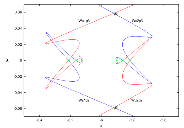
A.3 Computation of transversal homoclinic points and splitting angle
In this appendix, we compute the angle between the invariant manifolds at one of the transversal intersections. We will restrict the range of energy values to
| (93) |
or equivalently the range of eccentricities to . This is the range where we can validate the accuracy of our computations (see Appendix A.4). Below , the splitting size becomes comparable to the numerical error that we commit in double precision arithmetic.
Remark A.4.
In this paper we concentrate on proving the existence of global instabilities in the Restricted three-body problem; we are not so much concerned with finding the maximal range of eccentricities along which the asteroid drifts. Thus we do not investigate the transversality of the splitting below . However, we are convinced that the maximal range of eccentricities is larger than , in particular that the lower bound can be pushed well below . We think that our mechanism of instability applies to this larger range of eccentricities. In fact, it is possible to study such exponentially small splitting using more sophisticated numerical methods, such as multiple-precision arithmetic, and high-order approximation of local invariant manifolds, see for instance [FS90, DRR99, GS08].

Consider first a fixed energy level that is close to the unperturbed situation, e.g. . The corresponding manifolds are given in Figure 12. In general, there are uncountably many intersection points. For instance, in Figure 11 we show six intersections on the symmetry line. However, when the perturbation is small, there is one distinguished intersection point located “in the middle” of the homoclinic. We call it the primary intersection point.
Let us compute the primary intersection point corresponding to the “outer” splitting of the manifolds and . For , the primary intersection corresponds to the first intersection of the manifolds with the line, as we grow the manifolds from the fix points. Thanks to the symmetry, it is enough to look for the intersection of with the axis, because must also intersect the axis at the same point.
To compute the intersection point , we continue using a linear approximation of the local manifold, and propagate a fundamental domain in the local manifold by iteration. Let be the unstable eigenvector associated to the point . Consider the fundamental segment between the points and , as in the previous section. First we look for the smallest natural such that intersects the axis. Then we use a standard numerical method (bisection-like one-dimensional root finding) to find a point in the fundamental segment such that
Thus we obtain the homoclinic point in Figure 12. Numerically, we verify that is in the the axis within tolerance.

Finally, we vary energy and use a continuation method to obtain the family of primary intersections , using as seed the primary intersection found above. See Figure 13.
Remark A.5.
For low energy levels (such as ), corresponding to weak hyperbolicity, the invariant manifolds behave as if they were close to integrable, and the primary intersection corresponds to the first intersection of the manifolds with the axis. For high energy levels (such as ), corresponding to strong hyperbolicity, the manifolds develop some folds, and thus the primary intersection may not correspond to the first intersection of the manifolds with the axis. See Figure 11.
In practice, we first identify the primary intersection at low energy levels, and then use a continuation method to obtain the primary family of intersections up to high energy levels.
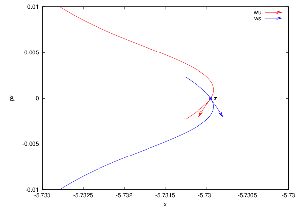
Analogously, we compute the family of primary intersections corresponding to the inner splitting. See Figure 13.
Let us now compute the splitting angle between the manifolds and at the point . For illustration, we show some numerical results corresponding to the energy value . First we need the tangent vectors and to the manifolds at . See Figure 14. As found above, let be the point in the unstable fundamental segment that maps to , i.e. . Consider the tangent vector to the manifold at the point . (Recall that at this point the linear approximation is good enough, so we can use as the unstable eigenvector.) Multiply by the Jacobian of at the successive iterates , for . This way, we obtain the tangent vector to the unstable manifold at . Let us denote this vector . We normalize it to .
Due to reversibility, the vector tangent to the stable manifold at is . See Figure 14. Notice that we choose the tangent vectors with the appropriate orientation, i.e. with the same orientation as the trajectories on the manifolds.
Thus the oriented splitting angle between and is
where is the arctangent function of two variables, which uses the signs of the two arguments to determine the sign of the result.

| inner | outer |
|---|---|
Finally, we let change and, using this procedure, we are able to obtain the splitting angle for energy levels . See Figure 15. The splitting angle is nonzero for all energy values except for a discrete set of them. The splitting angle oscillates around zero with decreasing amplitude as . Numerically, we find that the zeros of the splitting angle are contained in the intervals listed in Table 1.
Notice that the inner and outer splittings behave similarly. However, they become zero at different values of , as seen in Table 1. Thus, when one of the intersections becomes tangent, the other one is still transversal, and we can always use one of them for diffusion.
A.4 Accuracy of computations
For small eccentricities, the splitting angle becomes very small. We need to check the validity of , making sure that the size of (accumulated) numerical errors in the computation is smaller than the size of .
The smallest splitting angle in Figure 15, corresponding to , is
We check the validity of by recomputing this angle using an alternative numerical method. First we compute the intersection of the manifolds and with the horizontal axis defined by
for .
In Table 2 we tabulate the coordinate of and on these axes, and their difference gives the distance between the manifolds. We apply numerical differentiation to the last column of this table, using central differences centered at with step sizes and , and obtain the values:
Finally, we use Richardson extrapolation and obtain:
Thus, using this alternative method, we obtain the splitting angle
Compare the splitting angle computed using the two methods. They differ by approximately . This gives an estimate of the numerical error commited in our computation of the splitting angle.

We repeat this test for a range of energies . In Figure 16, we compare the splitting angle and the estimate of the numerical error . This error stays below , and it is several orders of magnitude smaller than the splitting angle. For higher energy values , the splitting angle is large, so the numerical error is certainly smaller. Therefore we are confident that the splitting angle has been accurately computed in the range of eccentricities considered, .
Appendix B Numerical study of the inner and outer dynamics
In Appendix A we have studied the periodic orbits and the invariant manifolds in rotating Cartesian coordinates . Nevertheless, the study of the inner and outer maps are done in rotating Delaunay coordinates. Indeed since these coordinates are action-angle coordinates for the two body problem, it is much more convenient to use them to study the mean motion resonance.

The Poincaré section is completely different from the section which will be used from now on (see (21)). In particular, the periodic orbits obtained in Appendix A.1 intersect the section six times whereas they intersect seven times. However, we remark that the homoclinic points and lie on the symmetry axis both in Cartesian and in Delaunay variables. See Figures 17 and 18.
To obtain the intersection of these periodic orbits with we just need to express the -periodic points of the Poincaré map obtained in Appendix A.1 in Delaunay coordinates and then iterate them by the flow of the circular problem expressed in Delaunay coordinates until they hit the section . We do the same with the homoclinic points. In Appendix B.1 we explain how to compute the change of coordinates and the vector field in Delaunay coordinates. Then, in Appendices B.2 and B.3 we study the inner and outer maps of the circular and elliptic problems respectively. Finally, in Appendix B.4 we compare the inner and outer maps of the elliptic problem, which leads to Ansatz 3.

B.1 From Cartesian to Delaunay and computation of
We explain an easy way to obtain the rotating Delaunay coordinates from rotating Cartesian (or polar) coordinates in the circular problem. First recall that can be computed as
The potential in Cartesian coordinates only depends on the position of the asteroid, and can be easily computed. Then, one can use the equation
to obtain . Knowing and we can obtain the eccentricity by
Using that , one can obtain and from here using Kepler’s equation . On the other hand, from we can obtain using
Finally, we can deduce using that .
We devote the rest of this appendix to compute . The other derivatives of can be computed analogously. Let us define
Then
Thus by the chain rule there only remains to compute and . First, let us point out that
On the other hand, using that , one has that
Then, since , using that
| (94) |
we have that
and therefore,
To compute , let us point out that . Therefore it only remains to compute , we obtain it using formula (94) and
Then,
and therefore,
B.2 Inner and outer dynamics of the circular problem
In this appendix, we numerically compute the inner map and the outer maps of the circular problem, given in Section 2. Recall that to compute these maps we deal with the extended system given by the Hamiltonian in (16) with restricted to the energy level and thus, we have that . Then, we consider , where the range is given in (93).
As seen in Section 2.2, the inner map has the form
| (95) |
where is the period of the periodic orbit obtained in Ansatz 1 on the corresponding level of energy , which now corresponds to an invariant hyperplane .
Recall that we computed the periodic orbit as well as its period in Appendix A.1. In particular, Figure 6 shows a plot of the function . Notice that the derivative of the function is nonzero for the whole range . This shows that the inner map is twist. Moreover, Figure 6 shows that
Therefore, the function satisfies the properties stated in Lemma 2.
As a test, we have computed the same function using two different methods. First by computing the period of the periodic orbit, as above. Then by computing the integral expression (38) using numerical integration. The difference in using both methods is of the order .

As seen in Section 2.3, the outer maps have the form
| (96) |
For simplicity, let us only discuss the computation of ( is computed analogously). Recall from Lemma 2.6 that the function is defined as
where, taking into account that the homoclinic orbit is symmetric with respect to the involution (19),
| (97) |
with
| (98) |
| (99) |
To obtain , we compute the integrals (98) and (99) numerically, using a standard algorithm from the GSL library [GG09]. The integrals are computed within a relative error limit .
The function involved in both integrals is given explicitly in Appendix B.1. The integral is evaluated on a periodic trajectory of the reduced circular problem (namely, with reparameterized time, see (30)) with initial condition , a fixed point of the Poincaré map . The integral is evaluated on a homoclinic trajectory of the reduced circular problem with initial condition , the primary homoclinic point corresponding to the inner splitting found in Appendix A.3.

Next we make a couple of important remarks about the numerical computation of the integral . The key point is that the homoclinic orbit was already computed in Appendix A.3 with high accuracy, and we can exploit this information here. Recall that the primary homoclinic point was obtained as the -th iterate of a point in the local fundamental segment under the Poincaré map:
| (100) |
Moreover, recall that the point was chosen to be suitably close to the fixed point for each energy level . See Remark A.3.
Notice that the integral is defined by a limit as , i.e. as the homoclinic orbit asymptotically approaches the periodic orbit in forward time (see equation (39)). Numerically, of course, we should stop integrating at an upper endpoint large enough such that the integral converges. In practice, we choose the upper endpoint to be the number of iterates in (100). This means that we evaluate the integral along the homoclinic trajectory until it reaches the point , which is suitably close to the periodic orbit.
Notice also that integrating the homoclinic trajectory forwards in the reduced system means integrating it backwards along the unstable manifold in the original system. This is numerically unstable, since numerical errors grow exponentially. In practice, we rewrite the integral (98) using the change of variables so that the homoclinic trajectory is integrated forwards along the unstable manifold, starting from the point .
The computed values of the functions and are shown in Figure 19. Note that they are plotted as a function of the Jacobi constant instead of as a function of , so that they can be compared with Figure 6, where we have plotted as a function of .
To test the computation of the function , we directly verify the definition of the outer map in 2.3. Let be the primary homoclinic point, and let be the periodic point. Given a point in the extended circular problem, we check that it is forward asymptotic (in the reparametrized time) to the point , where is arbitrary. Thus we check that the distance
with exponential decay.
The result of the test is shown in Figure 20 for values of the energy (recall that ). Notice that the vertical axis is in logarithmic scale. Let . We plot the distance as a function of (multiples of the period). The test shows exponential decay of the distance function for all energy values, i.e. straight lines in the plot.
Recall that the periodic orbits become more hyperbolic as the energy decreases. Thus, the rate of exponential convergence between the homoclinic and the periodic trajectory also increases, i.e. the straight lines have increasing slope in the plot. As explained above, the length of integration along the homoclinic orbit is suitably chosen for each energy level. For , there is exponential decay up to time .
B.3 Inner and outer dynamics of the elliptic problem
In this appendix, we numerically compute the first orders in of the inner map and the outer maps of the elliptic problem, given in Section 3. In order to compare the inner and outer dynamics of the elliptic problem through Lemma 4.2, only some specific terms in the expansions of the inner and outer maps are necessary. Namely, we only need to compute the term in the expansion of the inner map (61), and the terms in the expansion of the outer maps (72).

Recall from Section 3.4 that can be split as
Since and are complex conjugate, it is only necessary to compute one of them. Let us compute the positive harmonic,
| (101) |
Notice that the denominator is the same one used in the previous section for the inner and outer dynamics of the circular problem. Next we give the numerator explicitly. Let
where is the function defined in Lemma 3.4. Then it is straightforward to see that
| (102) |
where

The computed value of the function is shown in Figure 21. We plot it as a function of the energy of the elliptic problem in rotating coordinates in (15). Recall that since we are working in the energy level of the extended Hamiltonian in (16), we have that .
For the outer map, we compute the functions . Similarly to , it is only necessary to compute the positive harmonics . Recall from Lemma 3.9 that the positive harmonics and are defined as
| (103) |
where and were obtained in Appendix B.2. To obtain and , we compute the integrals (74)–(76) numerically, using the same techniques as in the previous Appendix B.2. In particular, the integrands of the Melnikov integrals (74) and (75), by construction, decay exponentially as and we take the same approximate limits of integration where is the constant considered in Appendix B.2.
The computed values of the functions and are shown in Figure 22.
B.4 Comparison of the inner and outer dynamics of the elliptic problem
Finally, we verify the non-degeneracy condition
| (104) |
stated in Lemma 4.2, which implies the existence of a transition chain of tori. Since and are complex-conjugate, it is only necessary to compute one of them. Let us compute the positive harmonic,
All the functions involved in the expression above are known: and are obtained in Appendix B.2 and and are obtained in Appendix B.3.

Appendix C The Main Result for the resonance: instabilities in the Kirkwood gaps
We devote this appendix to show how the proof of Theorem 1 in Sections 2–4 can be adapted to deal with the resonances. First, we state a more rigorous version of Main Result .
Theorem 5.
Ansätze 4 and 5 are stated in Appendix C.1 and Ansatz 6 is stated in Appendix C.2. They are analogous to Ansätze 1, 2 and 3 but referred to the resonance instead of the one. To prove this theorem, we consider the Hamiltonian (16) and we study the resonance
| (105) |
As for the resonance, without loss of generality, we take and we look for a large drift in , which being almost constant, implies a big drift in .
C.1 The circular problem
We first study the circular problem (18), close to the resonance . We assume the following ansatz. It has been verified numerically (see Appendix C.3). It replicates Ansatz 1.
Ansatz 4.
Consider the Hamiltonian (18) with . Then, in each energy level , there exists a hyperbolic periodic orbit of period which satisfies
and is smooth with respect to , and
for all .
Each has two branches of stable and unstable invariant manifolds and , . Then, for each either and or and intersect transversally.
Note that since now Jupiter is slower than the Asteriod, the period of the these periodic orbits is approximately the period of Jupiter instead of the period of the asteroid. For the Extended Circular Problem given by the Hamiltonian (16) with , the periodic orbits obtained in Ansatz 4 become invariant two-dimensional tori which belong to hyperplanes for any
Corollary C.1.
Assume Ansatz 4. Then, the Hamiltonian (16) with and has an analytic normally hyperbolic invariant -dimensional manifold , which is foliated by two-dimensional invariant tori.
Moreover, has two branches of stable and unstable invariant manifolds, which we call and , . Then, in the invariant planes , for each either and or and intersect transversally.
For the analysis of the resonance is more convenient to consider the global Poincaré section instead of the section considered in Section 2, since now the asteroid moves faster than Jupiter. We consider the map
| (106) |
induced by the flow associated to the Hamiltonian (16) with . Now the intersection of the cylinder with the section is formed by three cylinders , . Namely,
| (107) |
As a whole is a normally hyperbolic invariant manifold for the Poincaré map whereas each is a normally hyperbolic invariant manifold for . These cylinders have a natural system of coordinates, which we use to study the inner and outer dynamics on them. We work with and since in each invariant plane they are connected by at least one heteroclinic connection (of ) which is symmetric with respect to the involution (19). As before, we call it a forward heteroclinic orbit if it is asymptotic to in the past and in the future and a backward heteroclinic orbit if it is asymptotic to in the past and to in the future. We denote by , where stands for forward, the subset of where and intersect transversally and by , where stands for backward, the subset of where and intersect transversally. By Corollary C.1 we have that .
Corollary C.2.
Assume Ansatz 4. Then, the Poincaré map defined in (106), which is induced by the Hamiltonian (16) with and , has three analytic normally hyperbolic invariant manifolds , . They are foliated by one-dimensional invariant curves. Moreover, there exist analytic functions ,
that parameterize , namely,
The associated invariant manifolds and intersect transversally provided ; and and intersect transversally provided . Moreover, one of the points of these intersections belongs to the symmetry axis of (19). Let us denote by , , these intersections. Then, there exist analytic functions
which parameterize them:
Corollary C.1 gives global coordinates for each cylinder . These coordinates are symplectic with respect to the canonical symplectic form . We consider the inner and the two outer maps in the cylinder .
The inner map
The inner map is defined as the Poincaré map restricted to the symplectic invariant submanifold . It is of the form
| (108) |
where the function is such that is the period of the periodic orbit obtained in Ansatz 4 on the corresponding energy surface. We assume the following ansatz, which asserts that this map is twist (see the corresponding Ansatz 2). It has been verified numerically (see Appendix C.3).
Ansatz 5.
The function satisfies
Therefore, the analytic symplectic inner map is twist. Moreover, the function satisfies
The outer map
Proceeding as in Section 2.3, we define the outer map for the circular problem at the resonance. Recall that it has been defined as a composition of the map given by Definition 2.3 and a suitable power of the Poincaré map restricted to the cylinders . For the resonance, we consider outer maps , , which connect to itself and are defined as
where is the outer map which connects and through and is the outer map which connects and through . Recall that we are abusing notation since the forward and backwards outer maps are only defined provided and respectively and not in the whole cylinder .
As for case, these maps are of the form
| (109) |
Since we want to compute these outer maps using flows, we need to reparameterize time in the vector field associated to the Hamiltonian (16) with , so that it preserves the section . We consider the following vector field, which corresponds to identifying the variable with time,
| (110) |
where is Hamiltonian (16) with . Notice that now we are not changing time direction, as happened in the resonance. We refer to this system as a reduced circular problem. Recall that we denote by the flow associated to the components of equation (30) (which are independent of and ). We use it to derive the formulas for the outer map. Let
| (111) |
be trajectories of the circular problem. Then, one can see that the functions involved in the definition of the outer maps in (109) can be defined as
where
| (112) |
with
| (113) |
and
| (114) |
where is the function in (108). Recall that along the periodic and homoclinic orbits .
C.2 The elliptic problem
We study now the elliptic problem. Reasoning as for the resonance, for small enough the system associated to the Hamiltonian (16) has a normally hyperbolic invariant cylinder , which is -close to given in Corollary 2.1. Analogously, the Poincaré map
associated to the flow of (16) and the section has a normally hyperbolic invariant cylinder . Moreover, it is formed by three connected components , , which are -close to the cylinders obtained in Corollary C.2 and have natural coordinates as happened for the circular case.
We look for perturbative expansions of the inner and outer maps. For the resonances they are computed using the new reduced elliptic problem
| (115) |
which is a perturbation of (110).
For the elliptic problem, the coordinates are symplectic not with respect to the canonical symplectic form but whith respect to a symplectic form
| (116) |
with certain functions which satisfy
(see (84) for the definition of and Corollary 3.8 for the corresponding result for the resonance).
In the invariant cylinder , one can define inner and outer maps as we have done in for the circular problem. We proceed as in Section 3 for the resonance.
The inner map
We study first the inner map. As for the circular problem, it is defined the map in (41) restricted to the normally hyperbolic invariant manifold . For small enough, proceeding as in the proof of Lemma 3.7, one can see that it is of the form
| (117) |
with functions , and satisfying
| (118) | ||||
| (119) |
Thus, can be split as,
Moreover, the Fourier coefficients are defined as
where the functions are defined as
and has been defined in (111). Finally, is defined as
| (120) |
where has been introduced in Corollary C.2 and
| (121) |
The function is analogous to the corresponding function for the resonance, defined in (36).
The outer map
We study now the outer maps
| (122) |
for . Thanks to Ansatz 4, we know that for small enough, there exist transversal intersections of the invariant manifolds of and . Thus, we can proceed as in Section 2.3 to define the outer maps for the resonance and we study them as a perturbation of the outer maps of the circular problem given in (109). We use the reduced elliptic problem defined in (115) and we compute their first order. To this end, we use the notation and defined in (111). Analogously we define their corresponding -component of the flow as
| (123) |
Lemma C.3.
Existence of diffusing orbits
The last step to prove the existence of diffusing orbits can be done analogously to what has been done in Section 4 for the resonance. Namely, we just need to obtain a change of coordinates which
- 1.
Straightens the symplectic form (see (116)) into .
- 2.
Flattens the inner map in the -direction.
This is summarized in the next lemma, which merges the corresponding Lemmas 4.1 and 4.2 for the resonance.
Lemma C.4.
To be able to ensure the existence of transition chains of tori, we need to assume the following ansatz.
Ansatz 6.
C.3 Numerical study of the resonance
In this section, we briefly describe our numerical analysis of the resonance. In particular, we verify Ansätze 4, 5 and 6 numerically.
The numerical methodology used for the resonance is analogous to the resonance. Cartesian rotating coordinates are used for the computation of the hyperbolic structure of the circular problem (normally hyperbolic invariant cylinder, stable and unstable manifolds, and their homoclinic intersection). We now consider the Poincaré section
and the associated -dimensional symplectic Poincaré map acting on . We now look for resonant periodic orbits as -periodic points of the Poincaré map, i.e. letting , we need to solve the equation
In fact, exploiting the symmetry of the problem, it is enough to use -dimensional root finding:
since we impose that the point lies on the symmetry section .

Thus we obtain the family of resonant periodic orbits for energy levels
See Figure 24. Notice that the period stays close to the resonant period of the unperturbed system. From Figure 24, we obtain the bound
which is the first bound given in Ansatz 4.

Furthermore, we verify that (the square of) the semi-major axis stays close to the resonant value . Integrating the periodic orbit in Delaunay coordinates over one period , we compute the quantity
| (131) |
The function is plotted in Figure 24. Notice that we obtain the bound
for all and , which is the second bound given in Ansatz 4.
To determine the stability of the periodic orbits, we now compute the eigenvalues and of . Figure 25 shows the characteristic exponents , as a function of energy. The family of periodic orbits is hyperbolic in the interval , although the strength of hyperbolicity is weaker than in the resonance. Compare with Figure 7.

The stable and unstable invariant manifolds of the periodic orbits are computed using the same methodology explained for the resonance. In particular, we switch to the new Poincaré section
in order to have the homoclinic points lying on the symmetry axis. For illustration, we show the result corresponding to the energy value in Figure 26. The manifolds intersect transversally at the homoclinic points (outer splitting) and (inner splitting), as we will show below.
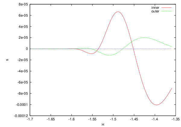
Next we compute the splitting angle between the invariant manifolds at the homoclinic points. We will restrict the range of energy values to
| (132) |
or equivalently the range of eccentricities to . This is the range where we can validate the accuracy of our computations (see Appendix A.4). Below , the splitting size becomes comparable to the numerical error that we commit in double precision arithmetic.
Remark C.5.
In contrast with the resonance, now the manifolds stay close to the integrable situation for the whole range of energies, i.e. they meet with small splitting angle as we will show below. Thus for the resonance there is no difficulty in identifying the primary family of homoclinic points. Compare with Remark A.5.
| inner | outer |
|---|---|
Using the same methodology as for the resonance, we are able to obtain the splitting angle for energy levels . See Figure 27. Numerically, we find that the zeros of the splitting angle are contained in the intervals listed in Table 3. As seen from the table, the inner and outer splittings become zero at different values of . Thus, when one of the intersections becomes tangent, the other one is still transversal, and we can always use one of them for diffusion.

Again, we check the validity of by computing this splitting angle using two different numerical methods and comparing the results. They differ by less than , which gives an estimate of the total numerical error.
Recall that the study of the inner and outer maps is done in rotating Delaunay coordinates. As explained in Appendix C, for the analysis of the resonance it is convenient to consider the Poincaré section . Thus, we transform the hyperbolic structure of the circular problem from Cartesian to Delaunay coordinates as explained in Appendix B.1. See Figure 28.
First we compute the inner map and the outer maps of the circular problem, given in Appendix C.1. We consider , where the range is given in (132). For the inner map, Figure 24 shows a plot of the function . Notice that the derivative of the function is nonzero for the whole range . This shows that the inner map is twist. Moreover, Figure 24 shows that
Therefore, the function satisfies the properties stated in Ansatz 5.
Then we compute the first orders in of the inner map and the outer maps of the elliptic problem, given in Appendix C.2. For brevity, we do not show the results here, since the plot of the functions , and does not convey much information.

Appendix D Conjectures on the speed of diffusion
Instabilities for nearly integrable systems are often called Arnol’d diffusion. As far as we know, this term was coined by Chirikov [Chi79]. In this section we state two conjectures about random behavior of orbits near resonances, where randomness is coming from initial condition.
A nearly integrable Hamiltonian systems of two degrees of freedom in the region of interest often can be reduced to a two-dimensional area-preserving twist map. To construct instability regions of these maps physicists often use a resonance overlap criterion (see e.g. [SUZ88], ch. 5, sect. 2). This criterion for nearby rational numbers and compares “sizes” of averaged potentials. If the sum of square roots of maxima of those potentials exceeds , this is a strong indication that the corresponding periodic orbits can be connected. Doing this for an interval of rational numbers gives an approximation for a so-called Birkhoff Region of Instability (BRI).
If non-integrability is small, then most of the space is laminated by KAM invariant curves. In order to find channels outside of KAM curves, one considers a neighborhood of a resonance and computes size of a so-called stochastic layer. Heuristic formulas can be found e.g. in [Chi79], ch. 6.2 or in [SUZ88], ch. 5, sect. 3. Treschev [TZ10] estimated width of stochastic layer in a fairly general setting.
It turns out that Arnol’d’s example and the elliptic problem near mean motion resonances can be viewed as a perturbation of a product of two area-preserving twist maps. In loose terms, for the first map we study orbits located near a resonance inside the corresponding stochastic layer. Width of a stochastic layer gives an approximation for time it takes for many orbits to go around the layer. Stochastic behavior for the other twist map occurs because it takes place “over” stochastic layer with random behavior. This randomness gives rise to “random compositions” of twist maps. Numerical experiments show behavior similar to a diffusion process (see e.g. [LL10, Figure 6.3] or [LFG07]). Its diffusion coefficient is proportional to square of the properly averaged perturbation divided by (see e.g. [Chi79], ch. 7.2, [SUZ88], ch.5, sect. 7).
However, mathematically such randomness is a dark realm since there are many phenomena competing with the diffusive behavior. For example, for twist maps here are a few serious obstacles:
- •
inside of a BRI there are elliptic islands, where orbits are confined and do not diffuse (see e.g. [Chi79], ch. 5.5 for a heuristic discussion of their size);
- •
even if elliptic islands occupy not a dominant part of the phase space, there exist the so-called, in mathematical literature, Aubry-Mather sets. In physics literature they are called Cantor-Tori. Orbits can stick to these sets for long periods of time (see e.g. [SUZ88], ch.5, sect. 7);
- •
similarly to sticking to Aubry-Mather sets orbits can stick to elliptic islands.
For systems of two and a half degrees of freedom near a resonance is also quite complicated. We turn to our attention to two basic examples: Arnol’d’s example and the elliptic problem, both near a resonance.
In terms of a perturbation parameter of a nearly integrable system one would like to answer quantitatively the following natural questions. Fix a resonant segment and consider a -neighborhood of this resonant segment.
- •
What is the natural time scale of diffusion? One would expect that there is an -dependent time scale in which one orbit diffuses by in action space and there is another time scale in which many orbits, in the measure sense, diffuse by .
- •
Is there a natural time scale so that positive fraction of orbits in a -dependent region in diffuses by ?
- •
At junctions of two resonances which fraction of orbits chooses one resonance over the other?
Call time scale of diffusion. It seems a sophisticated question to distinguish orbits starting in and staying inside such a neighborhood in time scale of diffusion from those getting stuck near KAM tori located -away 99 9 This is so-called stickiness phenomenon (see e.g. [MG95, PW94]) from with large. In this paper we consider only the a priori unstable case, proposed by Arnol’d [Arn64]. In this case, away from small velocities, there is only one dominant resonance and making precise conjectures is simpler. This case will also motivate conjectures for certain a priori chaotic systems.
D.1 Speed of diffusion for a priori unstable systems and Positive measure
Consider the following nearly integrable Hamiltonian system proposed by Arnol’d [Arn64]:
| (133) |
for an analytic perturbation . This system is usually called a priori unstable. Proving Arnol’d diffusion for this system consists in showing that, for all small and a generic , there exists orbits with
where is independent of . There has been a fascinating progress in this problem achieved by several groups (see [Ber08, CY04, DdlLS06, DH09, Tre04]). Treschev [Tre04] not only proved existence of Arnol’d diffusion, but also gave an optimal estimate on speed, namely, he constructed orbits
for some . One can see that this estimate is optimal, i.e. for some .
Heuristically the mechanism of diffusion is the following. For small the Hamiltonian has a -dimensional normally hyperbolic invariant cylinder close to . A hypothetical diffusing orbit starts close to and makes a homoclinic excursion. Each homoclinic excursion takes approximately -time. Increment of after such an excursion is .1010 10 This is only an heuristic description as dynamics inside of the cylinder should come into play. Near so-called double resonance dynamics is different from the one near single resonances If one can arrange that all excursions lead to increments of of the same sign, the result follows.
It seems natural that orbits will be trapped inside
the resonance for polynomially long time.
Using this heuristic description one can conjecture
that increments can behave as a random walk
for positive conditional measure for polynomially
large time.
Positive measure conjecture Consider the Hamiltonian with a generic perturbation . Pick an -ball of initial conditions, whose center projects into , and denote the Lebesgue probability measure supported on it by . Then, for some constants independent of , the set of initial conditions satisfying
is denoted Diff and has measure
.
Since a typical excursion takes -time and each increment is , we essentially conjecture that after excursions with uniformly positive probability there will be drift of order .
D.2 Structure of the restricted planar elliptic three-body problem
In this appendix we relate a priori unstable systems and the restricted planar elliptic three-body problem. Recall that we managed to write the Hamiltonian of the latter problem in the form
We have that
- •
is an integrable Hamiltonian.
- •
is non-integrable and for in a certain interval of energy levels there is a family of hyperbolic periodic orbits whose invariant manifolds intersect transversally along at least one homoclinic.
- •
is a -perturbation of such that certain Melnikov integral evaluated along a transverse homoclinic of is non-degenerate in two different ways: dependence on time is non-trivial and relation between inner and outer integrals is non-degenerate (see (9)).
Having all these non-degeneracy conditions we prove the existence of diffusing orbits. It is not difficult to prove, using averaging techniques, that for small, there is a family of saddle periodic orbit on some interval , whose hyperbolicity is . It seems, however, to be a non-trivial problem to establish the splitting of its separatrices. Due to reversibility (90) there are at least four homoclinic intersections (two for upper separatrices and two for lower ones). Having these two conditions it is natural to expect that at least one of the four associated Melnikov integrals is non-degenerate. Qualitative analysis shows that it should be possible to have a homoclinic excursion -close to the invariant cylinder. Such an excursion takes -time. If the excursion is selected properly, then the result of the excursion is that the increment of the eccentricity is . This makes us believe that the instability time obeys stated in (6).
Let us point out that we believe that our diffusion mechanism survives even for non-infinitesimal ’s, e.g. realistic . To justify this, we review the above structure.
Notice that we use a -dimensional normally hyperbolic invariant cylinder and the intersection of its invariant manifolds to diffuse. The cylinder arises from the family of periodic orbits of the circular problem, which persist under the elliptic time-periodic perturbation (see (15) and the derivation in the corresponding section). As the analysis carried out in Section 3.2 shows, in the neighborhood of this family , the perturbation can be averaged out to . Thus, invariant cylinders could persist even for not very small ’s. However, estimating remainders analytically after several steps of averaging is nearly impossible. Numerically though it might be feasible.
Once the existence of an invariant cylinder is established, we need to justify the existence of transverse intersections of its manifolds. As before, analytically it is an insurmountable task, but numerically it seems to be an achievable goal.
If these two steps are done, then one could try to compute numerically inner and outer maps and show that they do not have common invariant curves. This is again a difficult, but numerically realistic task (see [DMR08] for the computation of the outer map in another problem in Celestial Mechanics).
On the other hand, the above asymptotics probably does not hold in the neighborhood of circular motions of the massless body, which might be much more stable than more eccentric motions. Yet many other factors might influence the local stability or instability of various objects (see section 1.2.3).
D.3 The Mather accelerating problem and its speed of diffusion
The structure we use to build diffusion is similar to the Mather acceleration problem. Let us recall this problem and state an interesting result of Piftankin [Pif06] on speed of diffusion.
Consider a Hamiltonian system
where — kinetic energy corresponding to a riemannian metric and is a time-periodic potential energy. Since the system is not autonomous energy is not conserved.
- H1
-
Suppose the geodesic flow associated to has a hyperbolic periodic orbit and transversal intersection of its invariant manifolds, which contains a homoclinic orbit .
- H2
-
The Melnikov integral is not constant. More exactly, define a function
The limit turns out to exist and is independent of a choice of . This function is assumed to be non-constant.
Mather and his followers [Mat96, BT99, DdlLS00, GT08, Kal03, Pif06] proved existence of an orbit of unbounded energy. De la Llave [dlL04], Piftankin [Pif06], and Gelfreich-Turaev [GT08] proved that such an orbit can be chosen to have linear growth of energy
for some and .
Notice that for large energies the conformal change of coordinates
leads to the new Hamiltonian
It was shown in [dlL04, Pif06, GT08] that there are orbits diffusing linearly in the size of the perturbation. In order to see these orbits, notice that has a horseshoe. Then, can be considered as a time-periodic perturbation over such a horseshoe. It is shown by different methods in [dlL04, Pif06, GT08] that for a generic time-periodic perturbation of a horseshoe there are linearly diffusing orbits.
D.4 Modified positive measure conjecture
For systems with the properties discussed above we can modify the positive measure conjecture as follows:
Positive measure conjecture for Mather type systems Consider the Hamiltonian
such that
- •
for some interval the Hamiltonian has a family of saddle periodic orbits ,
- •
for each there is at least one transverse intersection of its invariant manifolds,
- •
A Melnikov integral evaluated along a transverse homoclinic and inner dynamics are non-degenerate: the dependence of the Melnikov integral on time is non-trivial and the relation between inner and outer maps is non-degenerate (see (9)).
Pick a -ball of initial conditions whose action components are centered at a resonance between and . Denote the Lebesgue probability measure supported on the ball by . Then for some constants independent of and , the set of initial conditions satisfying
is denoted Diff and has measure
.
Here is an important difference between the system and an priori unstable one , given by (133): the Hamiltonian already has “chaos” and a family of horseshoes on each energy surface with , while is integrable. As we pointed out above, for a generic time-periodic perturbation over a horseshoe there are orbits diffusing linearly fast [dlL04, Pif06, GT08]. Yet we are interested in a set of conditional positive measure.
In order to see the time of diffusion on an heuristic level, notice that has a family of saddle periodic orbits whose exponents are . Thus, one homoclinic excursion passing -close to separatrices takes -time. Each excursion might lead to increment of of size . Conjecturing that random walk approximation holds true to have -changes in , we need excursions.
Acknowledgements
The authors acknowledge useful discussions with Abed Bounemoura, Marc
Chaperon, Alain Chenciner, Anatole Katok, Àngel Jorba, Mark Levi,
John Mather, Gennadi Piftankin, Philippe Robutel and Ke Zhang. P. R.
acknowledges the assistance of À. Jorba with the “taylor” package
(see http://www.maia.ub.es/~angel/taylor).
The authors warmly thank the Observatoire de Paris, the University of Maryland at College Park, the Pennsylvania State University, the Universitat Politecnica de Catalunya and the Fields Institute for their hospitality, stimulating atmosphere, and support.
J. F. has been partially supported by the French ANR (Projets ANR-12-BS01-0020 WKBHJ and ANR-10-BLAN 0102 DynPDE), M. G. and P. R by the Spanish MCyT/FEDER grant MTM2009-06973 and the Catalan SGR grant 2009SGR859, and V. K. by NSF grant DMS-0701271.
References
- [AKN88] V.I. Arnold, V.V. Kozlov, and A.I. Neishtadt. Dynamical Systems III, volume 3 of Encyclopaedia Math. Sci. Springer, Berlin, 1988.
- [Arn63] V. I. Arnold. Small denominators and problems of stability of motion in classical and celestial mechanics. Uspehi Mat. Nauk, 18(6 (114)):91–192, 1963.
- [Arn64] V.I. Arnold. Instability of dynamical systems with several degrees of freedom. Sov. Math. Doklady, 5:581–585, 1964.
- [BB02] M. Berti and P. Bolle. A functional analysis approach to Arnold diffusion. Ann. Inst. H. Poincaré Anal. Non Linéaire, 19(4):395–450, 2002.
- [BBB03] M. Berti, L. Biasco, and P. Bolle. Drift in phase space: a new variational mechanism with optimal diffusion time. J. Math. Pures Appl. (9), 82(6):613–664, 2003.
- [Ber08] P. Bernard. The dynamics of pseudographs in convex Hamiltonian systems. J. Amer. Math. Soc., 21(3):615–669, 2008.
- [BKZ11] P. Bernard, V. Kaloshin, and K. Zhang. Arnold diffusion along normally hyperbolic cylinders. Preprint, 2011.
- [Bol06] S. Bolotin. Symbolic dynamics of almost collision orbits and skew products of symplectic maps. Nonlinearity, 19(9):2041–2063, 2006.
- [BT99] S. Bolotin and D. Treschev. Unbounded growth of energy in nonautonomous Hamiltonian systems. Nonlinearity, 12(2):365–388, 1999.
- [CC07] A. Celletti and L. Chierchia. KAM stability and celestial mechanics. Mem. Amer. Math. Soc., 187(878):viii+134, 2007.
- [CG94] L. Chierchia and G. Gallavotti. Drift and diffusion in phase space. Ann. Inst. H. Poincaré Phys. Théor., 60(1):144, 1994.
- [Cha04] M. Chaperon. Stable manifolds and the Perron-Irwin method. Ergodic Theory Dynam. Systems, 24(5):1359–1394, 2004.
- [Chi79] B. V. Chirikov. A universal instability of many-dimensional oscillator systems. Phys. Rep., 52(5):264–379, 1979.
- [Cre97] J. Cresson. A -lemma for partially hyperbolic tori and the obstruction property. Lett. Math. Phys., 42(4):363–377, 1997.
- [CY04] C.Q. Cheng and J. Yan. Existence of diffusion orbits in a priori unstable Hamiltonian systems. J. Differential Geom., 67(3):457–517, 2004.
- [CZ11] M. Capiński and P. Zgliczyński. Transition tori in the planar restricted elliptic three-body problem. Nonlinearity, 24(5):1395–1432, 2011.
- [DdlLS00] A. Delshams, R. de la Llave, and T.M. Seara. A geometric approach to the existence of orbits with unbounded energy in generic periodic perturbations by a potential of generic geodesic flows of . Comm. Math. Phys., 209(2):353–392, 2000.
- [DdlLS06] A. Delshams, R. de la Llave, and T.M. Seara. A geometric mechanism for diffusion in hamiltonian systems overcoming the large gap problem: heuristics and rigorous verification on a model. Mem. Amer. Math. Soc., 2006.
- [DdlLS08] A. Delshams, R. de la Llave, and T. M. Seara. Geometric properties of the scattering map of a normally hyperbolic invariant manifold. Adv. Math., 217(3):1096–1153, 2008.
- [DGR11] A. Delshams, M. Gidea, and P Roldán. Arnold’s mechanism of diffusion in the spatial circular restricted three-body problem: A semi-numerical argument. Preprint, 2011.
- [DH09] A. Delshams and G. Huguet. Geography of resonances and Arnold diffusion in a priori unstable Hamiltonian systems. Nonlinearity, 22(8):1997–2077, 2009.
- [dlL04] R. de la Llave. Orbits of unbounded energy in perturbations of geodesic flows by periodic potentials. A simple construction. Preprint, 2004.
- [DMR08] A. Delshams, J. Masdemont, and P. Roldán. Computing the scattering map in the spatial Hill’s problem. Discrete Contin. Dyn. Syst. Ser. B, 10(2-3):455–483, 2008.
- [DRR99] A. Delshams and R. Ramírez-Ros. Singular separatrix splitting and the Melnikov method: an experimental study. Experiment. Math., 8(1):29–48, 1999.
- [Féj02a] J. Féjoz. Global secular dynamics in the planar three-body problem. Celestial Mech. Dynam. Astronom., 84(2):159–195, 2002.
- [Féj02b] Jacques Féjoz. Quasiperiodic motions in the planar three-body problem. J. Differential Equations, 183(2):303–341, 2002.
- [Féj04] J. Féjoz. Démonstration du ‘théorème d’Arnold’ sur la stabilité du système planétaire (d’après Herman). Ergodic Theory Dynam. Systems, 24(5):1521–1582, 2004.
- [Féj13] J. Féjoz. On ”Arnold’s theorem” in celestial mechanics -a summary with an appendix on the Poincaré coordinates. Discrete and Continuous Dynamical Systems, 33:3555–3565, 2013.
- [Fen72] N. Fenichel. Persistence and smoothness of invariant manifolds for flows. Indiana Univ. Math. J., 21:193–226, 1971/1972.
- [Fen77] N. Fenichel. Asymptotic stability with rate conditions. II. Indiana Univ. Math. J., 26(1):81–93, 1977.
- [Fen74] N. Fenichel. Asymptotic stability with rate conditions. Indiana Univ. Math. J., 23:1109–1137, 1973/74.
- [FM00] E. Fontich and P. Martín. Differentiable invariant manifolds for partially hyperbolic tori and a lambda lemma. Nonlinearity, 13(5):1561–1593, 2000.
- [FS90] E. Fontich and C. Simó. The splitting of separatrices for analytic diffeomorphisms. Ergodic Theory Dynam. Systems, 10(2):295–318, 1990.
- [GDF+89] A. Giorgilli, A. Delshams, E. Fontich, L. Galgani, and C. Simó. Effective stability for a Hamiltonian system near an elliptic equilibrium point, with an application to the restricted three-body problem. J. Differential Equations, 77(1):167–198, 1989.
- [GdlL06] M. Gidea and R. de la Llave. Topological methods in the instability problem of Hamiltonian systems. Discrete Contin. Dyn. Syst., 14(2):295–328, 2006.
- [GG85] A. Giorgilli and L. Galgani. Rigorous estimates for the series expansions of Hamiltonian perturbation theory. Celestial Mech., 37(2):95–112, 1985.
- [GG09] M. Galassi and B. Gough. GNU Scientific Library: Reference Manual. A GNU manual. Network Theory Limited, 2009.
- [GK10a] J. Galante and V. Kaloshin. Destruction of invariant curves in the restricted planar circular three body problem using ordering condition. Preprint, 2010.
- [GK10b] J. Galante and V. Kaloshin. The method of spreading cumulative twist and application to the restricted planar circular three body problem. Preprint, 2010.
- [GK11] J. Galante and V. Kaloshin. Destruction of invariant curves in the restricted circular planar three-body problem by using comparison of action. Duke Math. J., 159(2):275–327, 2011.
- [GS08] V. Gelfreich and C. Simó. High-precision computations of divergent asymptotic series and homoclinic phenomena. Discrete Contin. Dyn. Syst. Ser. B, 10(2-3):511–536, 2008.
- [GT08] V. Gelfreich and D. Turaev. Unbounded energy growth in Hamiltonian systems with a slowly varying parameter. Comm. Math. Phys., 283(3):769–794, 2008.
- [Her83] M.R. Herman. Sur les courbes invariantes par les difféomorphismes de l’anneau. Vol. 1, volume 103 of Astérisque. Société Mathématique de France, Paris, 1983.
- [Her98] M. Herman. Some open problems in dynamical systems. In Proceedings of the International Congress of Mathematicians (Berlin, 1998), volume Extra Vol. II, pages 797–808 (electronic), 1998.
- [Kal03] V. Kaloshin. Geometric proofs of Mather’s connecting and accelerating theorems. In Topics in dynamics and ergodic theory, volume 310 of London Math. Soc. Lecture Note Ser., pages 81–106. Cambridge Univ. Press, Cambridge, 2003.
- [Kol57] A. N. Kolmogorov. Théorie générale des systèmes dynamiques et mécanique classique. In Proceedings of the International Congress of Mathematicians, Amsterdam, 1954, Vol. 1, pages 315–333. Erven P. Noordhoff N.V., Groningen, 1957.
- [Lap89] P.-S. Laplace. Variations séculaires des orbites des planètes. Mém. Acad. royale des sciences de Paris, année 1787, Œuvres complètes, Tome XI:295–301, 1789. http://gallica.bnf.fr/ark:/12148/bpt6k77599c/f300.
- [Las94] J. Laskar. Large scale chaos in the solar system. Astron. Astrophys., 287, 1994.
- [Las06] J. Laskar. Sfogliando La ‘Méchanique analitique’, chapter Lagrange et la stabilité du système solaire. Edizioni Universitarie di Lettere Economia Diritto, 2006.
- [Las10] J. Laskar. Le système solaire est-il stable ? In Le Chaos, number XIV in Séminaire Poincaré, pages 221–246. Birkhäuser, 2010.
- [LFG07] E. Lega, C. Froeschlé, and M. Guzzo. Diffusion in Hamiltonian quasi-integrable systems. In Topics in gravitational dynamics, volume 729 of Lecture Notes in Phys., pages 29–65. Springer, Berlin, 2007.
- [LL10] A.J. Lichtenberg and A. Lieberman. Regular and Chaotic Dynamics. Applied Mathematical Sciences. Springer, 2010.
- [Mar96] J. P. Marco. Transition le long des chaînes de tores invariants pour les systèmes hamiltoniens analytiques. Ann. Inst. H. Poincaré Phys. Théor., 64(2):205–252, 1996.
- [Mat96] J. N. Mather. Manuscript. Unpublished, 1996.
- [Mey75] K. R. Meyer. The implicit function theorem and analytic differential equations. In Dynamical systems—Warwick 1974 (Proc. Sympos. Appl. Topology and Dynamical Systems, Univ. Warwick, Coventry, 1973/1974; presented to E. C. Zeeman on his fiftieth birthday), pages 191–208. Lecture Notes in Math., Vol. 468. Springer, Berlin, 1975.
- [MG95] A. Morbidelli and A. Giorgilli. Superexponential stability of KAM tori. J. Statist. Phys., 78(5-6):1607–1617, 1995.
- [Moe96] R. Moeckel. Transition tori in the five-body problem. J. Differential Equations, 129(2):290–314, 1996.
- [Moe02] R. Moeckel. Generic drift on Cantor sets of annuli. In Celestial mechanics (Evanston, IL, 1999), volume 292 of Contemp. Math., pages 163–171. Amer. Math. Soc., Providence, RI, 2002.
- [Mor02] A. Morbidelli. Modern celestial mechanics: aspects of solar system dynamics. Taylor and Francis, 2002.
- [Nie96] L. Niederman. Stability over exponentially long times in the planetary problem. Nonlinearity, 9(6):1703–1751, 1996.
- [NS04] A. I. Neishtadt and V. V. Sidorenko. Wisdom system: dynamics in the adiabatic approximation. Celestial Mech. Dynam. Astronom., 90(3-4):307–330, 2004.
- [Pif06] G. N. Piftankin. Diffusion speed in the Mather problem. Nonlinearity, 19(11):2617–2644, 2006.
- [PT07] G. N. Piftankin and D. V. Treshchëv. Separatrix maps in Hamiltonian systems. Uspekhi Mat. Nauk, 62(2(374)):3–108, 2007.
- [PW94] A.D. Perry and S. Wiggins. KAM tori are very sticky: rigorous lower bounds on the time to move away from an invariant Lagrangian torus with linear flow. Phys. D, 71(1-2):102–121, 1994.
- [Rob05] P. Robutel. Frequency analysis and global dynamics of a planetary system. In D. Benest, editor, Hamiltonian systems and Fourier analysis: new prospects for gravitational dynamics, Advances in astronomy and astrophysics, pages 179–198. Cambridge Scientific Publishers, 2005.
- [Sab13] L. Sabbagh. An inclination lemma for normally hyperbolic manifolds with an application to diffusion. Preprint, 2013.
- [SM95] C. L. Siegel and J. K. Moser. Lectures on celestial mechanics. Classics in Mathematics. Springer-Verlag, Berlin, 1995.
- [SUZ88] R.Z. Sagdeev, D.A. Usikov, and G.M. Zaslavskij. Nonlinear Physics: From the Pendulum to Turbulence and Chaos. Contemporary Concepts in Physics Series. Harwood Academic Publishers, 1988.
- [SW92] G. J. Sussman and J. Wisdom. Chaotic evolution of the solar system. Science, 257:56–62, 1992.
- [Tre04] D. Treschev. Evolution of slow variables in a priori unstable hamiltonian systems. Nonlinearity, 17(5):1803–1841, 2004.
- [TZ10] D. Treschev and O. Zubelevich. Introduction to the perturbation theory of Hamiltonian systems. Springer Monographs in Mathematics. Springer-Verlag, Berlin, 2010.
- [Wis82] J. Wisdom. The origin of the Kirkwood gaps: a mapping for asteroidal motion near the commensurability. Astronom. J., 87(3):577–593, 1982.
- [WZ03] D. Wilczak and P. Zgliczynski. Heteroclinic connections between periodic orbits in planar restricted circular three-body problem—a computer assisted proof. Comm. Math. Phys., 234(1):37–75, 2003.
- [Xue10] J. Xue. Continuous averaging proof of the nekhoroshev theorem with sharp stability constant . Preprint, Penn State University, 43 pp, 2010.
- [Zhe10] Y. Zheng. Arnold diffusion for a priori unstable systems and a five-body problem. Preprint, Penn State University, 51 pp, 2010.