Equilibria of biological aggregations with nonlocal repulsive-attractive interactions
Abstract
We consider the aggregation equation in , where the interaction potential incorporates short-range Newtonian repulsion and long-range power-law attraction. We study the global well-posedness of solutions and investigate analytically and numerically the equilibrium solutions. We show that there exist unique equilibria supported on a ball of . By using the method of moving planes we prove that such equilibria are radially symmetric and monotone in the radial coordinate. We perform asymptotic studies for the limiting cases when the exponent of the power-law attraction approaches infinity and a Newtonian singularity, respectively. Numerical simulations suggest that equilibria studied here are global attractors for the dynamics of the aggregation model.
Keywords: swarm equilibria, biological aggregations, Newtonian potential, global attractors
AMS Subject Classification: 92D25, 35L65, 35Q92, 35B35
1 Introduction
The multidimensional integro-differential equation,
| (1) |
has attracted a great amount of interest in recent years. The equation appears in various contexts related to mathematical models for biological aggregations, where represents the density of the aggregation and is the social interaction potential. The asterisk denotes convolution. We refer to [32, 34] for an extensive background and literature review on mathematical models of social aggregations and in particular, for a thorough discussion on the relevance of equation (1) for modelling swarming behaviours. The equation also arises in a number of other applications such as granular media [35, 12], self-assembly of nanoparticles [24, 25], Ginzburg-Landau vortices [16, 14, 31] and molecular dynamics simulations of matter [23]. In this work however we are primarily interested in biological applications, where equation (1) is used to model social aggregations such as insect swarms, fish schools, bacterial colonies, etc [32].
Regarded as a model for biological aggregations, equation (1) incorporates inter-individual social interactions such as long-range attraction and short-range repulsion, through the aggregation potential . The properties of the potential (symmetry, regularity, monotonicity, etc) are essential in studying issues such as the well-posedness [9, 6, 8] or the long-time behaviour [10, 28] of solutions to model equation (1). In particular, a large component of the research on this model dealt with attractive potentials which lead to solutions that blow-up (in finite or infinite time) by mass concentration, into one or several Dirac distributions [19, 4, 26].
It is essential however for an aggregation model to be able to capture solutions with biologically relevant features. As pointed out by Mogilner and Keshet in their seminal work [32] on the class of models discussed here, such desired characteristics include: finite densities, sharp boundaries, relatively constant internal population and long lifetimes. The difficulty in finding such solutions to model (1) has been indicated as a “challenge” in previous literature [33, 29], and in fact there is only a handful of works that address this issue. Topaz and collaborators [28, 3] derived explicit swarm equilibria that arise in the one-dimensional model with Morse-type potentials (in the form of decaying exponentials), but their explicit calculations do not extend to higher dimensions. Other works illustrate asymptotic vortex states in [33] and clumps (aggregations with compact support) in a nonlocal model that includes density-dependent diffusion [34].
A recent publication of the authors [20] considered an interaction potential for which equilibria of the aggregation model (1) have the desired characteristics indicated above. More specifically, the kernel investigated in [20] has a repulsion component in the form of the Newtonian potential and attraction given by a power law11 1 See Section 5 for a discussion on how the potential can be modified to avoid the biologically unrealistic growth of attraction with distance when .:
| (2) |
Here, is the free-space Green’s function of the negative Laplace operator :
| (3) |
and is a real exponent, . In (3), is the number of space dimensions and denotes the volume of the unit ball in .
We summarize briefly some of the results from [20] that are relevant to the present article. For , the equilibrium density of (1)-(2) is uniform inside a ball of and zero outside it. In this case, the method of characteristics was used to solve explicitly the dynamics corresponding to radially symmetric initial conditions in any dimension. This showed the global stability within the class of radially symmetric solutions of the constant steady state. The explicit calculations did not extend to general exponent , but the existence of a unique radially symmetric equilibrium of compact support was shown, after casting the equilibrium problem as an eigenvalue problem for an integral operator and applying the Krein-Rutman theorem. Some explicit calculations of the equilibria could be performed however for the special subcase when is even. In addition to these studies on equilibria, the global well-posedness of solutions to (1)-(2) (with ) was shown by borrowing techniques used in the analysis of incompressible Euler equations [30].
The main purpose of the work from [20] was to design attractive-repulsive potentials that yield equilibrium states of finite densities and compact support. In this respect, the attraction component of the potential was specifically designed to counter-balance the singular Newtonian repulsion. Newtonian (attractive) potentials for model (1) were considered in [14, 31] in the context of vortex motions in two-dimensional superfluids. The main concern of these works was the well-posedness of solutions, in particular concentration and singularity formation in measure-valued solutions. Very recently, Newtonian potentials were also considered in aggregation models [5, 7]. In [7], the authors study patch solutions and they consider separately the case of an attractive Newtonian potential (with finite time concentration) and of a repulsive Newtonian potential (with spreading to a circular/ spherical aggregation patch).
The purpose of the present research is (i) to extend the interaction potential (2)-(3) studied in [20] to allow for more general attractive forces22 2 In the special case we take . () and (ii) to investigate analytically and numerically the properties of the equilibria to the aggregation model (1)-(2) for . Remarkably, the intricate balance between the power-law attraction and the singular repulsion provides the model with a very interesting and at the same time biologically relevant set of steady states. For all values of , the aggregation model has a unique steady state supported in a ball. This steady state is radial and monotone in the radial coordinate. More specifically, the equilibria are decreasing about the origin for and increasing for , while corresponds to a constant equilibrium density. Figure 1 shows the equilibrium solutions in three dimensions for various values of ; all shown equilibria have mass 1. The limits and , that is, when attraction becomes infinitely strong (at large distances) or as singular as the (Newtonian) repulsion, are particularly interesting. As , the radii of the equilibria approach a constant, but the qualitative features change dramatically, as mass aggregates toward the edge of the swarm, leaving an increasingly void region in the centre — this effect can be observed in Figure 1 (). As , the radii of equilibria approach and mass concentrates at the origin – see Figure 1 (). Numerical simulations suggest that all these equilibria are global attractors for the dynamics of (1)-(2), which motivates and gives strong grounds to the studies of the present work.

There are a few very recent studies of equilibria of (1) with attractive-repulsive potentials in power-law form that closely relate to our work. In [1], the authors study the stability of spherical shell equilibria for potentials in the form , where (short range repulsion and long range attraction). While the attraction component, , is the same as in (2), the singularity of the repulsion term is “better” than Newtonian (). Shell steady states are shown to exist and be locally stable under certain conditions on the exponents and . The methods from [1] do not apply to Newtonian singularities. Other recent works that involve model (1) with power-law potentials focus on pattern formation and linear stability analysis of spherical shells [27, 37].
The results of the paper are as follows. Well-posedness of solutions to the aggregation model (1)-(2) (with ) is studied in Section 2 by using analogies with the incompressible fluid flow equations [30, 20, 7]. For all values of , we show in Section 3.1 that there exist unique equilibria supported on a ball of . In Section 3.2 we employ the method of moving planes [21] to prove that such equilibria are radially symmetric and monotone in the radial coordinate. In Section 4 we performed careful asymptotic and numerical investigations of the equilibria. Our studies address two issues. The first one is the behaviour of equilibria as and . As expected, the two limiting cases give very different asymptotic behaviours. The second issue addressed in Section 4 is the stability of the equilibrium solutions. The results regarding stability are preliminary and entirely based on numerical observations. Based on all numerical experiments we performed, we conjecture that the equilibria studied in this paper are global attractors for solutions to (1)-(2).
2 A priori bounds and well-posedness of solutions
We start by pointing out that the aggregation model (1)-(2) has two important conservation properties. Denote the initial density by :
(i) Conservation of mass:
| (4) |
where the constant denotes the initial mass .
(ii) Conservation of centre of mass:
| (5) |
where we assume, without loss of generality, that the centre of mass of the initial density is at the origin: .
Both properties follow directly from (1). Property (ii) uses the radial symmetry of the potential. The two conservation properties will be used frequently in this article.
By introducing the notation:
we write the aggregation model as
| (6a) | |||
| (6b) | |||
| (6c) | |||
This work makes extensive use of the Lagrangian formulation of the aggregation model (6), where dynamics is tracked along the characteristic curves, defined by:
| (7) |
2.1 A priori bounds on density
Expand and write the evolution of the density along characteristics:
| (8) |
The continuity equation (6a) expresses the fact that
| (10) |
where
is the Jacobian of the particle map .
Define the maximum of the density
We show that provided is bounded initially, it remains bounded above, uniformly in time. This was shown in [20] for and here we extend the results to include .
Let . From the characteristic equation (8) for and the expression (9) for , we have, along particle trajectories:
| (11) | ||||
| (12) |
where we used and will be chosen conveniently later. Use the following estimates on the integrals in the right-hand-side of (12):
and choose to be:
| (13) |
We find
with
resulting in the following inequality
| (14) |
As , the damping dominates the growth term in the right-hand-side of (14): . The right-hand-side of (14) becomes negative when and hence, regardless of the size of the support, the maximum density is bounded uniformly in time, provided it is initially bounded.
Remark. For , it was shown in [20] that the density has compact support uniformly in time, provided the initial density has compact support. This property was used to conclude global wellposedness of solutions. In the present study, where , we could not show the compact support of solutions when , but we managed to circumvent this by using the uniform -bound of .
We present briefly the argument that shows uniform compact support for . The density is transported along characteristics (see equation (10)), so it is enough to show that the trajectories that carry non-zero densities remain within some compact set. Calculate using (6b) and (6c):
| (15) |
Define the maximum radius of support as
and evaluate (15) at on the boundary of the support, i.e., for any such that . The left-hand-side of (15) becomes
We estimate the first term in the right-hand-side of (15) as follows:
For the second term, use and , for on the boundary of the support and in the support of , to find
where we used conservation of mass (4) and centre of mass (5) to go from the second to the last line. Using the estimates in (15), derive
Hence, the trajectories that carry non-zero densities will remain inside the disk of radius , where
2.2 Existence and uniqueness of solutions
To study well-posedness of solutions we use a Lagrangian approach and rewrite the aggregation equation (1) in terms of particle trajectories. Then we regard the model as an ODE on a certain Banach space and infer local existence and uniqueness from Picard theorem. The setup of the ODE framework is the same as that used in [20] to study the case and is inspired from the study of well-posedness of solutions to the incompressible Euler equation in Lagrangian formulation [30]. Extension to global existence is achieved through an argument similar to the well-known Beale-Kato-Majda blow-up criterion for incompressible flows [2].
Make the change of variable in the expression (6b) for , with given by (6c), and use (10) to write the characteristic equation (7) as
| (16a) | ||||
| (16b) | ||||
where the map is defined by
| (17) |
System (16)-(17) is a reformulation the PDE model (6) in terms of particle-trajectory equations. Case was studied in detail in [20], by analogy with the ODE setup of the incompressible Euler equations [30].
Following [30, 20], we consider the Banach space
where is the norm defined by
| (18) |
Here, is the Hölder seminorm
Consider an open subset , of defined by
The key ingredients to show local and global well-posedness of solutions are the properties of the convolution kernel
| (19) |
present in the repulsion component of (6c). In particular, is singular, homogeneous of degree and its gradient is homogeneous of degree and defines a singular integral operator (SIO). The close analogy with incompressible fluid equations comes from the fact that a similar kernel appears in the Biot-Savart law [30].
The local existence and uniqueness is stated by the following theorem.
Theorem 2.1.
Proof.
We now use a continuation result of solutions to autonomous ODE’s on Banach spaces (Theorem 4.4 in [30]) to upgrade the result to global existence. Inspecting the set we infer that we cease to have a solution at a finite time provided either becomes or becomes unbounded as .
The first scenario is ruled out by the following proposition.
Proof.
The second scenario for the break-up of the solution (finite-time blow-up of ) will be treated as in Chapter 4.2 of [30]. This procedure was used in [20] to study global well-posedness of solutions to (16), (17) when . In summary, can be shown to remain bounded for all finite times, provided , for all . This is an analogue of the Beale-Kato-Majda condition for global existence of solutions to incompressible Euler equations [2, 30]. Our argument is adapted from the analysis of the incompressible fluid equations presented in Chapter 4 of [30].
A first a priori bound is provided by the following proposition.
Proposition 2.3.
Provided has an a priori bound, and are a priori bounded.
Proof.
The Beale-Kato-Majda condition for global existence of incompressible Euler equations is an a priori control on the time-integral of the supremum norm of vorticity. In the context of our aggregation model (16)-(17), this condition will be replaced by an a priori bound on .
Proposition 2.4.
A sufficient condition for to be a priori bounded is an a apriori bound on . More specifically,
where is a constant that depends on the initial density only.
Proof.
Case was discussed in [20]. The proof for requires some slight adaptations from the corresponding result for fluids (see Theorem 4.3 and its proof in [30]). The repulsion component of can be estimated using (68). The attraction part has a milder singularity and does not break the estimate, hence we have
Set to get
Lemma 4.8 in [30] can be trivially adapted to our context, resulting in the following inequality:
By combining the last two inequalities we find
The desired inequality follows after division by and integration with respect to . ∎
Finally, we have all the ingredients to prove global existence of solutions. The result is given by the following theorem.
Theorem 2.5.
(global existence and uniqueness) Consider the trajectory equations (16), (17) with the Banach space setup and notations as above, and a compactly supported initial density , with , for some . Then, for every , there exists and a unique solution to (16), (17) with (a unique solution exists globally in time).
Proof.
Case was studied in [20] and we focus here on the range .
The solution is in the set provided
| (20) |
Using Proposition 2.2, the first condition is satisfied provided we choose . We now investigate the second condition in (20). Start by inspecting the first term in (18), . Integrate (7) to get
| (21) |
The repulsion component of can be bounded in terms of using (67). The attraction component also has a uniform bound. To show this we distinguish two cases: (i) and (ii) , and inspect the attraction part of , i.e., . In case (i),
In case (ii) solutions are compactly supported (uniformly in time) in a ball of radius , provided the initial density is — see Remark in Section 2.1. Hence,
Using (21) we derive
| (22) |
The control of now follows from (22), Propositions 2.3 and 2.4. More precisely, by redefining the constants appropriately, one can derive
| (23) |
Given that is uniformly bounded, we can choose the constant large enough such that , for all .
∎
3 Radially symmetric steady states
In this section we show that the aggregation model admits a unique radially symmetric steady state supported on a ball of . For , we prove that these steady states are monotonically decreasing about the origin, while for they are increasing about it. Case corresponds to constant solutions in a ball [20]. We further study these equilibria using numerical and asymptotic methods in Section 4.
3.1 Existence and uniqueness of equilibria supported on a ball
Suppose that is a steady state with support the ball centred at the origin, of radius . The velocity is zero in , so its divergence also vanishes. Hence, from (9) we find that satisfies the following integral equation,
| (24) |
and vanishes outside .
Consider the operator given by
| (25) |
The subscript is used to emphasize the dependence of the integral operator on the radius . As , the kernel is integrable and defines a linear bounded operator from to itself. Equation (24) can be cast as an eigenvalue problem,
where solutions are eigenfunctions corresponding to eigenvalue .
The existence and uniqueness of a steady state supported in is provided by the following theorem.
Theorem 3.1.
Proof.
We use a scaling argument and consider the case first. For , the kernel is integrable and the linear operator is bounded. The operator is also compact. This is a textbook exercise in analysis [36], but we include it here for completeness. Case presents no difficulty, as the kernel is continuous. For , we write as a limit of compact operators as follows. Consider a smooth cut-off function , such as for , for and for all . Define
and
The kernels are continuous, hence the operators are compact. Now estimate
As , , when . The convergence is uniform in , hence,
and is compact as a limit (in the operator norm) of compact operators.
We apply the Krein-Rutman theorem [15] to operator in the following setup. Take the cone in consisting of all non-negative functions. is a linear, strongly positive, compact operator that maps the space of continuous functions into itself. By Krein-Rutman theorem (see Theorem 1.2 in [15]), there exists a positive eigenfunction such that , where (which depends only on and ) is the spectral radius of . Moreover, the eigenvalue is simple and there is no other eigenvalue with a positive eigenvector. By making the change of variable
| (26) |
in (25), we get
Now ask that is an eigenfunction of corresponding to eigenvalue one and find
| (27) |
which gives the radius of the support as a function of and only. Once a mass for is set, uniqueness can be inferred from the uniqueness properties of the spectral radius of and its associated eigenfunction . ∎
3.2 Qualitative properties of equilibria
Monotonicity and radial symmetry of equilibria.
We prove that the equilibria given by positive solutions of (24) (and whose existence and uniqueness was established in Theorem 3.1) are radially symmetric and monotone in the radial coordinate. More specifically, equilibria are monotonically decreasing when and increasing for . To prove this result we employ the method of moving planes, a technique introduced by the Soviet mathematician Alexandroff in the early 1950’s, which became well-known after Gidas, Ni and Nirenberg [21] applied it to study qualitative properties of positive solutions of elliptic equations. We refer to [15] for a detailed description of the method and its applications.
Our use of the moving plane technique is inspired by a novel application of the method in the context of integral equations [13]. Consider a steady state supported on the ball ; satisfies the integral equation (24) in and vanishes outside . For convenience of calculations, denote
As , we have . Two cases will be distinguished from the subsequent analysis: (i) (equivalently, ) with radial equilibria which decrease about the origin, and (ii) (or ) with increasing solutions. Using the new notation, satisfies
| (28) |
Take such that , and consider the reflection across the plane , . In particular, we have the image of the origin under this map. Define
Using (28), is given by
| (29) |
Define
We apply the method of moving planes and compare and for . In case (i), , we show that there is a , , such that , for all . By a continuity argument, we show that the plane can be moved continuously all the way to , and hence, increases as approaches the origin from . A similar argument can be made using planes . Since the direction can be chosen arbitrarily we conclude that is radially symmetric and decreasing about the origin. For case (ii), , a similar argument leads to being radial and increasing about the origin.
Theorem 3.2.
Proof.
We use the notations and symbols introduced in the preamble of the theorem. Calculate , for . As outside , we have
It remains to consider the case . Denote by the complement of in , i.e.,
and calculate, using (28),
In the above calculation we used to write the second integral in the right-hand-side as an integral with respect to (subsequently relabelled ).
Similarly, using (29),
As is zero outside , the second integrals in the right-hand-sides of the expressions for and above can be extended to . Hence, we compute, for ,
| (30) |
Case (i) (or ): For and , . Hence,
| (31) |
Let us first assume that there exists such that
| (32) |
and prove that can be extended all the way to the origin . Suppose by contradiction that cannot be extended. Take , , and define
For , using (30) and (31) we find
and hence,
| (33) |
The function under the integral on the right-hand-side is integrable, as . Also, from (30), we infer that in the interior of , which implies that the closure of has measure . As , we conclude that the measure of approaches as . Therefore, we can choose small enough such that
By (33) we have =0, which implies that is empty, hence is not maximal and we reached the desired contradiction.
It remains to show that with the property (32) exists indeed. Note that (32) holds for (see (28) and (29)). An argument entirely similar to the one made in the previous step proves that the plane can be moved further to the right, while (32) still holds. This concludes the proof for case (i).
Case (ii) (or ) follows similarly, the single difference being the sign of the integrand in (30). More precisely, instead of (31), the reversed inequality holds:
A similar argument as that made for case (i) shows that decreases as approaches the origin from . Hence conclude that in this case is radially symmetric and increasing about the origin. ∎
Remarks
a. Case corresponds to constant solutions in a ball. These solutions were studied in detail in [20].
b. Theoretical findings are in perfect agreement with numerical results — see Section 4.
c. The convexity of the steady state can be inferred easily from (24) when (the function is convex for ).
4 Numerical and asymptotic studies of radial equilibria
We showed that a steady state supported on a ball is necessarily radially symmetric and monotone. In this section we investigate further their properties using numerical and asymptotic methods.
4.1 Numerical methods for the dynamic evolution and steady states
In solving numerically the steady states (24) or the dynamic evolution of solutions to (1)-(2), the computational bottleneck is the evaluation of the integral operators. The methods we use are similar to those in [26, 20] and are reviewed and extended below.
Steady states.
The equilibria are computed from (24) by using the power method [17], whose convergence is guaranteed by Theorem 3.1. First, write the operator given by (25) in radial coordinates:
| (34) |
where
| (35) |
The steady states are eigenfunctions of corresponding to eigenvalue . Here the eigenvalue problem consists in determining the eigenfunction and the radius of the support. The actual steady density is a constant multiple of this eigenfunction, where the constant is determined from the initial mass.
By the scaling argument used to prove Theorem 3.1 , it is enough to find the spectral radius of , and its corresponding eigenfunction ; the steady state can then be calculated from (27) and (26).
Given an initial positive density on , consider the iterative scheme (power method):
| (36) |
where can be any norm for functions on the unit interval . The sequence converges to [17], and the spectral radius of is given by the limit of , as goes to infinity.
The integral operator in (34) is discretized by the trapezoidal rule. The computational complexity can be reduced to the calculation of the integration in only, where can be interpolated using the fact that , where
| (37) |
and is computed at sample points on .
The calculations do not present significant challenges, except for , when is unbounded, making the error in the trapezoidal rule uncontrollable. We managed to calculate this more singular case only in dimensions one and three, where can be obtained explicitly. Due to these computational difficulties, the singular limit studied below by asymptotic methods is valid in all dimensions, but its numerical verification is done only in one and three dimensions.
In three dimensions for instance, the kernel from (35) can be calculated explicitly: when ,
| (38) |
and when or ,
Using the explicit form (38), when is in the singular range , and , the integrand in the integral operator (34) is weakly singular. However, the part associated with this weak singularity can be approximated as the product of the weakly singular function and a smooth function. When the latter is approximated by linear or higher order interpolation, the whole integral can be calculated explicitly[18], giving an accurate approximation of (34).
The steady states have been displayed in Figure 1 in dimension three, for a wide range of values of . The results are perfectly consistent with the monotonicity properties stated and proved in Theorem 3.2. As noted from Figure 1, equilibria display an interesting asymptotic behaviour as and . As , the radii of the equilibria approach a constant, and mass aggregates toward the edge of the swarm. As mass concentrates at the origin, as attraction becomes as strong as the Newtonian repulsion. We perform careful asymptotic studies in Section 4.2 and confirm and detail these observations.
Dynamic evolution to equilibria.
All numerical simulations we performed suggest that equilibria that solve (24) are global attractors for the aggregation model (1)-(2). To evolve dynamically the solutions to (1)-(2), we consider the model in characteristic form (see (16), (17), (11)). In radial coordinates the characteristic equations read
| (39a) | ||||
| (39b) | ||||
The term associated with the singular repulsion (the Newtonian potential ) in the right-hand-side of (39a) is calculated by taking advantage of the fact that the corresponding kernel is the fundamental solution of the Laplace equation.
Similar to the discretization of the integral from (34), the computational complexity in calculating the integrals from (39a) and (39b) can be reduced by introducing the following auxiliary functions: (defined by (37)),
Thus, the angular integrals in in (39a) and (39b) become products of powers of , , and these auxiliary functions, with . Hence the double integrals in (39a) and (39b) become single integrals in and are evaluated by trapezoidal rule. Due to the extra factor in the integrand, and are bounded for any , and can always be used in the trapezoidal rule. This observation reduces the total complexity in the computations to per time step, where is the number of spatial gridpoints in the radial coordinate . Once the characteristic speeds in (39) are found, the equations are evolved in time by the classical fourth order Runge-Kutta method.
Figures 2(a) and 2(b) show simulation results in three dimensions, corresponding to and , respectively. We plot the solution against the radial coordinate . The initial data used in Figure 2 is
| (41) |
where is a constant chosen to normalize the mass to one. The solutions approach as the steady states studied in Section 3 and shown in Figure 1. We note that for large , the convergence near the origin tends to be slow. Based on numerical observations we conjecture that these equilibria are global attractors for solutions to (1)-(2). In future work we plan to validate rigorously these observations regarding the global stability of the steady states.


| (a) (b) |
4.2 Asymptotic behaviour of equilibria as and
In general, there is no explicit formula for the radius of the support and the corresponding steady states on , governed by (24). However, when is large or close to the singular limit , the asymptotic behaviours can be obtained by perturbation expansions. To facilitate the exposition, we only consider the case and solve the eigenvalue problem
| (42) |
where
| (43) |
and vanishes outside . Provided we know the spectral radius of and its corresponding eigenfunction , the actual steady state in (24) can be recovered as , where and is a constant related to the total mass (see the proof of Theorem 3.1, in particular equations (26) and (27)).
In the rest of this section, the total mass for is assumed to be one. All asymptotic behaviours are investigated in one dimension first, to illustrate the essential techniques and features in a relatively simple setting, and then in higher dimensions.
Asymptotic limit when .
In this limit, the numerically computed eigenfunctions are observed to be concentrated near the boundary and the dominant contribution of the integral operator (43) comes from . This motivates the following asymptotic construction.
Start with the eigenvalue problem (42) in one dimension ():
| (44) |
When , the above integral on the right hand side is dominated at , that is
| (45) | ||||
| (46) |
For we find the same expression, considering the symmetry . Evaluate (44) at and use (46) to approximate its right-hand-side. We find and
| (47) |
where the coefficient is chosen such that the approximated has total mass one.
Approximations, as , to the actual steady states (with unit mass) and their support can be found from (26) and (27). Hence, . However, this is not an accurate approximation, as it can be observed from Figure 3(a), where we plot the radius against , as obtained from numerics (dots) and the above approximation (dashed line), the latter being referred to as the coarse approximation. To obtain the numerical results we used the methods described in Section 4.1.
The approximation of the eigenvalue can be improved considerably if in the right-hand-side of (44) one uses the expression of given by (47). Near , use to approximate the right-hand-side in (44). Then, evaluate at to find
The integral in the right-hand-side can be computed exactly and also, from (47), . We derive the refined approximation , with the corresponding radius,
| (48) |
The refined approximation, displayed as solid line in Figure 3(a) shows an excellent agreement with the numerical results (dots). Note that (the coarse approximation), as , but the convergence is slow.
Formally, the eigenfunction (47) can be regarded as obtained from the power method iteration (36), by starting with a constant initial guess . The coarse approximation of the eigenvalue is exactly , while the refined approximation is . Here the norm is the function evaluation at , i.e., . The same idea is applied below in higher dimensions, even though the expressions are much more complicted. This fact also illustrates the fast convergence of the iterative scheme (36) for large .
We also compare the steady states, as obtained by numerics (see methods in Section 4.1) and asymptotics (expression (47)). Figure 3(b) shows an excellent agreement between the two solutions for and .


| (a) (b) |
In higher dimensions, the eigenvalue problem can be approximated in a similar manner. Based on numerical observations, we assume that most contribution in the integral from (43) comes from the boundary. Hence, the eigenvalue problem for is approximated by
| (49) |
In general, the integral on the right-hand-side can not be integrated explicitly in the natural radial coordinates. However, when the origin is shifted to , we have
| (50) |
The approximation to the eigenvalue is obtained by evaluating expression (49) at , which gives
| (51) | ||||
| (52) |
where Beta and are the beta and Gamma functions, respectively.
The radius of the support can then be approximated as using Stirling’s approximation,
We refer to the outcome of this procedure as the coarse approximation and we plot the result in Figure 4(a) (dashed line). Note the low accuracy of this approximation, when compared to the numerical calculation (dots). The coarse approximation approaches however, as , the correct value , but the convergence is extremely slow.
The eigenfunction is approximated from (49):
| (53) |
where is a normalization constant determined by the total mass.
Similar to the 1D case, using the explicit approximation (53) of the eigenfunction, one can improve considerably the approximation of the corresponding eigenvalue (and hence of ), by substituting (53) into (49) and evaluating at . The outcome of this improved procedure is referred to as the refined approximation and is plotted (solid line) in Figure 4(a). The agreement of the refined approximation with the numerical results is now excellent. There is also a very good agreement between the eigenfunctions computed numerically (see Section 4.1) and their asymptotic approximation provided by (53) — see Figure 4(b).
Remark. Since the integral expression (53) for the approximation of is concentrated at , we can use Laplace’s method to find the leading order when is away from zero. Since , and for ,
the eigenfunction can be further approximated away from the origin as
However, this expression breaks down for near the origin and approximation (53) is used instead in the plot from Figure 4(b).
To conclude, the asymptotic study as shows that the radii of support of the equilibria (24) converge (slowly) to a fixed value , while the density concentrates to a -sphere of radius 0.5. We also point out that this asymptotic behaviour applies to all dimensions .


| (a) (b) |
Asymptotic limit when .
We write
and perform an asymptotic study in the small regime. We start with solutions in one dimension first, where the eigenvalue problem (42) reads
| (54) |
Here the subscript and superscript is used to emphasize the dependence of the eigenvalue and the corresponding eigenfunction on . The asymptotic expansion suggested from numerical simulation is
| (55a) | |||
| (55b) |
The kernel is not integrable in the limit when , and thus we can not substitute the formal expansions into (54) directly. Hence, it is not possible to carry out a straightforward expansion. However, using the fact that
the governing equation (54) can be written as
| (56) |
Now using the asymptotic expansions (55a) and (55b), we obtain
| (57a) | ||||
| (57b) | ||||
| (57c) | ||||
| (57d) | ||||
The first equation (57a) yields and the second equation (57b) is an eigenvalue problem for the limiting profile . Integrating the equation (57b) with respect to , we can get an alternative expression for the eigenvalue as
| (58) |
Even though we do not expect any explicit solutions to (57b), we can discretize and solve it using inverse iteration [22]. The condition , motivated from the numerical calculation of the steady states, is used to get rid of the singularity on the boundary. The initial data for the inverse iteration can be taken as the steady state calculated numerically from (54) with close to zero (and initial guess of the eigenvalue from (58) with replaced by ). This inverse power iteration normally converges in just a few steps.
The solution of (57d) is more challenging. Since this first order correction does not provide much insight into the problem, we focus instead on the second order correction of the eigenvalue . By the solvability condition for (57d), the right hand side of (57d) is orthogonal to , giving
| (59) | ||||
| (60) |
Figure 5(a) shows the normalized steady states for (corresponding to ), as computed numerically from the eigenvalue problem (54) using the methods described in Section 4.1. In the same figure we also plot (plain solid line) the leading order term of the expansion (55b), obtained by solving (57b) with the inverse iteration method. The plot confirms that the equilibria approach the limiting profile as .
In Figure 5(b) we plot (dots) the eigenvalues for various values of (corresponding to ), computed directly from (54) using the power method (Section 4.1). The dashed line represents the asymptotic approximation of from (55a) that includes second order corrections ( is computed from (58) and from (60). The agreement between the two sets of results for small ’s is excellent.


| (a) (b) |
At a closer inspection, it becomes clear that the expansion (55b) may be non-uniform near the boundary . In Figures 6(a)-(b) we plot evaluated at and , respectively, for different values of . The eigenfunctions are computed directly from (54) — see also Figure 5(a). At the origin (Figure 6(a)) we find a linear dependence on , as the approximation is uniform. However, at , we find , hence the expansion (55b) is non-uniform near the boundary (Figure 6(b)). To find a valid asymptotic expansion near one has to introduce a boundary layer and perhaps use the method of matched asymptotics to relate the inner and outer expansions. We do not pursue this direction here.


| (a) (b) |
The situation in higher dimensions is similar. We write the eigenvalue problem (42) as
| (61) |
where we used again subscripts and superscripts to emphasize the dependence on , and the auxiliary function is defined by
The auxiliary function can be simplified by shifting the origin (see the calculation leading to (50)), with the result:
where we also used a Taylor expansion in to expand . The term can be simplified using the the following calculation:
Hence,
| (62) |
where
Since the integrand in (61) is integrable provided is Hölder continuous, by introducing the formal asymptotic expansion (55) in (61) and using (62), one finds
| (63a) | ||||
| (63b) | ||||
| (63c) | ||||
| (63d) | ||||
Therefore, the leading order of the eigenvalue is and the limiting steady state and the first order correction can be solved by inverse iteration. The second order correction can be obtained from the solvability condition:
| (64) | ||||
| (65) |
In Figure 7 we test the asymptotic results in three dimensions. The qualitative behaviour of the steady states and their corresponding eigenvalues is similar to what has been observed in one dimension (Figure 5).
Figure 7(a) shows the normalized steady states for (corresponding to ) obtained by solving numerically (42), along with the limiting profile (plain solid line) found by inverse iteration from (63b). The asymptotic results are confirmed, as equilibria approach the limiting profile for . In Figure 7(b) we test the asymptotic expansion (55a) at order (dashed line) against the numerical solution of (42) (dots). The agreement is excellent for small or equivalently, for close to the critical value .

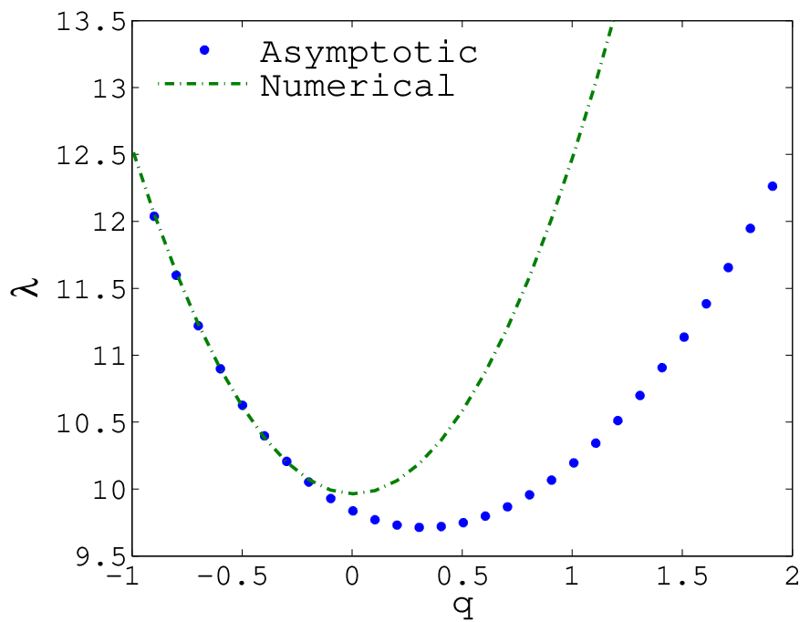
| (a) (b) |
Remark. An implication of the above study is that, in all dimensions, the radius vanishes exponentially fast as , and as a result, the true steady state converges to a Dirac delta function.
5 Discussion
We have studied the aggregation model (1) with potentials that contain short-range Newtonian repulsion and long-range power-law attraction. The main merit of the family of potentials considered here is that it leads to solutions which have biologically relevant features, such as finite densities, sharp boundaries and long lifetimes [32]. Finding such solutions to model (1) has been indicated as a “challenge” in previous works [33, 29] and the literature addressing this issue has been very scarce.
Well-posedness of solutions to (1) was studied by analogy with incompressible fluid equations [30], using the Lagrangian (particle) formulation of the model. The main object of the present work, i.e., equilibria supported on a ball, was investigated through a variety of analytical, numerical and asymptotic methods applied to the integral equation (24). We derived existence and uniqueness of such equilibria using the Krein-Rutman theorem and established qualitative properties such as monotonicity and radial symmetry, by the method of moving planes.
The numerical results confirm the analytical findings and also suggest that the equilibria studied in this work are global attractors for the dynamics of (1). We formulate this observation as a conjecture and we plan to address it in future work. A possible approach is to use the fact that the aggregation equation (1) represents a gradient flow with respect to the energy
However the energy is not convex, therefore its global minimizers cannot be characterized easily. Some recent progress in this direction was done in [11] in the context of aggregation models with long-range attraction and quadratic diffusion.
The asymptotic results revealed some very interesting features of solutions to (24). In particular, as the exponent of the power-law attraction approaches , the radii of the support approach a constant value , and the density concentrates on a -sphere. Distributions on spheres (uniform, as well as surprisingly complex patterns) have been studied recently [37, 1] using potentials with power-law repulsion and attraction. Concentrations on -spheres typically represent equilibrium solutions of the aggregation model. It is not surprising in fact that the non-convex energy has multiple stationary points, adding to the difficulties in studying its equilibria, as indicated before. Aggregations on spherical shells could be stable or unstable, depending on the exponents of the repulsive and attractive power-laws [27, 1]. Choosing the repulsion component in Newtonian form, as in this paper, seems to rule out concentrations on spheres from the possible asymptotic behaviours of solutions to (1), except in the limit .
The limit of solutions to (24) is interesting for its own sake. Weakly singular integral operators are subjects of many articles and textbooks (see [36] and references therein), but a careful asymptotic study of the eigenvalue problem (24), as the singularity approaches the critical value , is missing from the literature. We studied the scaled problem (42) for and showed that eigenvalues approach a constant, while the corresponding eigenfunctions approach a limiting profile , as (see Figures 5 and 7). Consequently, from the scaling (26)-(27), solutions to (24) approach a Dirac in the limit. The findings are consistent with works that consider blow-up in aggregation models with purely attractive potentials [19, 4], in particular recent works that consider Newtonian potentials [7].
Finally, we want to comment briefly on the biologically unrealistic feature of the potential (2), that is, the growth of attraction with distance, when . As discussed in more detail in [20], the dynamics of (1) remains unchanged if the potential is modified in an arbitrary way outside a ball of , with a sufficiently large radius that depends on the initial conditions only. This can be inferred from the property of the density to have uniform (in time) support; this property was shown to hold for and it is believed to hold for all in fact. Provided the radius of the support of the density is bounded by , where depends only on the initial conditions, but not on time, the potential can be taken to be zero (or exponentially decaying) for , without changing the dynamics. We refer the reader to [20] for a numerical illustration of this issue.
6 Appendix
Proof of Theorem 2.1
We show that the operator is bounded, i.e., , for all . We outline the main steps and refer to Chapter 4 [30] for details and various technical calculus inequalities.
Write as
Using the calculus inequality (Lemma 4.1 [30])
| (66) |
we estimate:
As for , it remains to bound , , and .
We first inspect the repulsion component of (see (6b), (6c) and (19)) and estimate , and , where and is the principal-value SIO:
The first of these terms can be bounded as follows:
| (67) |
To bound we follow the proof of Lemma 4.6 [30]. We split the integral:
The kernel has mean-value zero on the unit sphere,
which enables us to rewrite as
Hence
and
Here and below, denotes a generic constant. For the second integral, we estimate
Conclude
| (68) |
Finally, using the same argument as in Lemma 4.6 [30], one can show
| (69) |
Estimate the seminorm as in the proof of Proposition 4.2 [30], by using (10) and calculus inequality (66):
| (70) |
Using the calculus inequalities
| (71) |
| (72) |
from Lemmas 4.3 and 4.2 [30], respectively, estimate
and
As , and . Return to (70) to find:
Using the above bound on and the uniform bound on derived in Section 2.1, we infer from (67)-(69) that the repulsion component of yields a bounded operator. The singularity of the attraction component is milder than that of the repulsion and does not break the existing estimates for the singular repulsion kernel . We conclude that is bounded.
To prove that is Lipschitz continuous, we show that is bounded as a linear operator from to , i.e., , for all . Calculate using (17) and (6c):
| (73) |
where we suppressed the time dependence for convenience.
To estimate the component of due to repulsion one could follow the proof of Lemma 4.10 in [30]. The attraction component is milder and does not break the estimates. It can be shown that
which proves the boundedness in the operator norm of .
A key observation is that the term in (73) compensates for the singularity of . We present here the estimate of , which requires in fact some changes to the proof of Lemma 4.10 [30]. We do not present the estimates of and , we refer instead to the calculations in [30].
Use a change of variable, , , and split the repulsion component of from (73)
The procedure is similar to what we did to derive (67). From mean-value theorem, we have
As ,
where we also used (72), , and the uniform bound on in the second inequality.
The outer integral satisfies
where we used conservation of mass.
Combine the two estimates for and and argue that the attraction component would not break these estimates, to find
References
- [1] D. Balagué, J. A. Carrillo, T. Laurent, and G. Raoul. Nonlocal interactions by repulsive-attractive potentials: radial ins/stability. (preprint).
- [2] J. T. Beale, T. Kato, and A. Majda. Remarks on the breakdown of smooth solutions for the -D Euler equations. Comm. Math. Phys., 94(1):61–66, 1984.
- [3] Andrew J. Bernoff and Chad M. Topaz. A primer of swarm equilibria. SIAM J. Appl. Dyn. Syst., 10(1):212–250, 2011.
- [4] Andrea L. Bertozzi, José A. Carrillo, and Thomas Laurent. Blow-up in multidimensional aggregation equations with mildly singular interaction kernels. Nonlinearity, 22(3):683–710, 2009.
- [5] Andrea L. Bertozzi, John B. Garnett, and Thomas Laurent. Characterization of radially symmetric finite time blowup in multidimensional aggregation equations. (preprint).
- [6] Andrea L. Bertozzi and Thomas Laurent. Finite-time blow-up of solutions of an aggregation equation in . Comm. Math. Phys., 274(3):717–735, 2007.
- [7] Andrea L. Bertozzi, Thomas Laurent, and Leger Flavien. Aggregation via the Newtonian potential and aggregation patches. (preprint).
- [8] Andrea L. Bertozzi, Thomas Laurent, and Jesus Rosado. theory for the multidimensional aggregation equation. Comm. Pur. Appl. Math., 64(1):45–83, 2011.
- [9] M. Bodnar and J. J. L. Velazquez. An integro-differential equation arising as a limit of individual cell-based models. J. Differential Equations, 222(2):341–380, 2006.
- [10] Martin Burger and Marco Di Francesco. Large time behavior of nonlocal aggregation models with nonlinear diffusion. Netw. Heterog. Media, 3(4):749–785, 2008.
- [11] Martin Burger, Marco Di Francesco, and M Franek. Stationary states of quadratic diffusion equations with long-range attraction. 2011. (preprint).
- [12] José A. Carrillo, Robert J. McCann, and Cédric Villani. Contractions in the 2-Wasserstein length space and thermalization of granular media. Arch. Ration. Mech. Anal., 179(2):217–263, 2006.
- [13] Wenxiong Chen, Congming Li, and Biao Ou. Classification of solutions for an integral equation. Comm. Pure Appl. Math., 59(3):330–343, 2006.
- [14] Qiang Du and Ping Zhang. Existence of weak solutions to some vortex density models. SIAM J. Math. Anal., 34(6):1279–1299 (electronic), 2003.
- [15] Yihong Du. Order structure and topological methods in nonlinear partial differential equations. Vol. 1, volume 2 of Series in Partial Differential Equations and Applications. World Scientific Publishing Co. Pte. Ltd., Hackensack, NJ, 2006.
- [16] Weinan E. Dynamics of vortex liquids in Ginzburg-Landau theories with applications to superconductivity. Physical Review B, 50(2):1126Ð1135, 1994.
- [17] Sean Eastman and Donald Estep. A power method for nonlinear operators. Appl. Anal., 86(10):1303–1314, 2007.
- [18] P. P. B. Eggermont. A new analysis of the trapezoidal-discretization method for the numerical solution of Abel-type integral equations. J. Integral Equations, 3(4):317–332, 1981.
- [19] Klemens Fellner and Gaël Raoul. Stable stationary states of non-local interaction equations. Math. Models Methods Appl. Sci., 20(12):2267–2291, 2010.
- [20] R. C. Fetecau, Y. Huang, and T. Kolokolnikov. Swarm dynamics and equilibria for a nonlocal aggregation model. Nonlinearity, 24(10):2681–2716, 2011.
- [21] B. Gidas, Wei Ming Ni, and L. Nirenberg. Symmetry and related properties via the maximum principle. Comm. Math. Phys., 68(3):209–243, 1979.
- [22] Gene H. Golub and Charles F. Van Loan. Matrix computations. Johns Hopkins Studies in the Mathematical Sciences. Johns Hopkins University Press, Baltimore, MD, third edition, 1996.
- [23] J.M. Haile. Molecular Dynamics Simulation: Elementary Methods. John Wiley and Sons, Inc., New York, 1992.
- [24] Darryl D. Holm and Vakhtang Putkaradze. Aggregation of finite-size particles with variable mobility. Phys Rev Lett., 95:226106, 2005.
- [25] Darryl D. Holm and Vakhtang Putkaradze. Formation of clumps and patches in selfaggregation of finite-size particles. Physica D., 220(2):183–196, 2006.
- [26] Yanghong Huang and Andrea L. Bertozzi. Self-similar blowup solutions to an aggregation equation in . SIAM J. Appl. Math., 70(7):2582–2603, 2010.
- [27] Theodore Kolokolnikov, Hui Sun, David Uminsky, and Andrea L. Bertozzi. A theory of complex patterns arising from 2D particle interactions. Phys. Rev. E, Rapid Communications, 84:015203(R), 2011.
- [28] Andrew J. Leverentz, Chad M. Topaz, and Andrew J. Bernoff. Asymptotic dynamics of attractive-repulsive swarms. SIAM J. Appl. Dyn. Syst., 8(3):880–908, 2009.
- [29] Dong Li and Jose Rodrigo. Finite-time singularities of an aggregation equation in with fractional dissipation. Comm. Math. Phys., 287(2):687–703, 2009.
- [30] Andrew J. Majda and Andrea L. Bertozzi. Vorticity and incompressible flow, volume 27 of Cambridge Texts in Applied Mathematics. Cambridge University Press, Cambridge, 2002.
- [31] Nader Masmoudi and Ping Zhang. Global solutions to vortex density equations arising from sup-conductivity. Ann. Inst. H. Poincaré Anal. Non Linéaire, 22(4):441–458, 2005.
- [32] A. Mogilner and L. Edelstein-Keshet. A non-local model for a swarm. J. Math. Biol., 38:534–570, 1999.
- [33] C. M. Topaz and A. L. Bertozzi. Swarming patterns in a two-dimensional kinematic model for biological groups. SIAM J. Appl. Math., 65:152–174, 2004.
- [34] C. M. Topaz, A. L. Bertozzi, and M. A. Lewis. A nonlocal continuum model for biological aggregation. Bull. Math. Bio., 68:1601–1623, 2006.
- [35] Giuseppe Toscani. One-dimensional kinetic models of granular flows. M2AN Math. Model. Numer. Anal., 34(6):1277–1291, 2000.
- [36] Gennadi Vainikko. Multidimensional weakly singular integral equations, volume 1549 of Lecture Notes in Mathematics. Springer-Verlag, Berlin, 1993.
- [37] James von Brecht, David Uminsky, Theodore Kolokolnikov, and Andrea Bertozzi. Predicting pattern formation in particle interactions. (preprint).