ULB-TH/10-18

Re-reheating, late entropy injection and constraints from baryogenesis scenarios

Germano Nardini Affiliation: Service de Physique Théorique, Université Libre de Bruxelles, 1050 Brussels, Belgium Narendra Sahu Affiliation: Service de Physique Théorique, Université Libre de Bruxelles, 1050 Brussels, Belgium

Abstract

Many theories of particle physics beyond the Standard Model predict long-lived fields that may have dominated the Universe at early times and then decayed. Their decay, which injects entropy in the thermal bath, is responsible for a second reheating, dubbed re-reheating, that could substantially dilute the matter-antimatter asymmetry created before. In this paper we analyze such late re-reheating and entropy dilution. It turns out that in some cases the usual analytic calculation badly fails if it is not rectified by some corrective factors that we provide. We also determine the parameter space where the entropy dilution compromises models of baryogenesis. This region can be obtained by imposing some generic constraints that are applicable to any baryogenesis mechanism and long-lived field satisfying a few assumptions. For instance, by applying them to MSSM electroweak baryogenesis, thermal non-resonant leptogenesis and thermal resonant leptogenesis, we obtain that the initial abundances of long-lived fields with lifetime longer than respectively $5\times 10^{13},10^{-2}$ and $10^{15}\,{\rm\ GeV}^{-1}$ are strongly constrained. Similarly, the same baryogenesis scenarios are incompatible with large oscillations of moduli with mass smaller than $\mathcal{O}(10^{8}),\mathcal{O}(10^{13})$ and $\mathcal{O}(10^{7}){\rm\ GeV}$ that are naturally coupled to the visible sector via gravitational dimension-five operators.

pacs

98.80.Cq

I Introduction

The history of the Universe before Big Bang Nucleosynthesis (BBN) is an open issue. The standard cosmological scenario considers epochs prior to BBN to be radiation dominated. However, this assumption is questionable since experiments cannot put severe constraints on the Universe at temperature $T\gg\mathcal{O}(1\,$ MeV) and moreover several theoretical frameworks predict a modification of the standard cosmological picture. For instance, models having long lived fields that are not in thermal equilibrium may induce an era where the radiation energy is subdominant. Potentially, this epoch might emerge in presence of flat directions [1], Q-balls [2], gravitinos [3], axinos [4], moduli [5], which we will generically refer to as $X$ field in the following.

On the other hand, the history of the Universe at $T\lesssim\mathcal{O}(1\,$ MeV) is well established: any primordial $X$ -dominated epoch must end before the onset of BBN in order not to jeopardize the predictions of the primordial element abundances [6, 7]. The required return to the radiation dominated era may occur via $X$ decay. This process, which we dub re-reheating to distinguish it from the first reheating happened in the inflationary epoch, dumps entropy into the thermal bath and may considerably dilute the pre-existing species.

Various experimental observations can be explained by re-reheating. Among many we mention the possibility of tuning the $X$ -decay rate to generate the right amount of non-thermal cold dark matter required for structure formation [8]. Moreover, the $X$ decay can be invoked to wash out unwanted relics of early stages of the Universe (e.g., monopoles and domain walls), to circumvent the gravitino problem [9] or to reduce an overabundance of thermal dark matter candidates [10].

All these possibilities highlight that future detection of new particles might provide a link between (non-standard) cosmology and particle physics that might be misunderstood if non classical cosmological scenarios are not taken into account. Thus, in order to infer cosmological issues from particle experiments, we will need to clarify as much as possible the picture of the Universe before BBN. In particular, bounds on the possible $X$ -dominated epoch will be useful ¹¹ 1 Some constraints on $X$ are deduced by noticing that the $X$ decay might have left a trace in the Cosmic Microwave Background (CMB) [11]. Unluckily, such a signature cannot be disentangled from the inflaton one so that the derived bounds on $X$ depend strongly on the assumed inflationary model.. With this goal in mind, in the present paper we link the puzzle of the observed Baryon ( $B$ ) Asymmetry of the Universe (BAU) with the $X$ decay. In this manner we obtain some bounds on models involving baryogenesis and late-time entropy injection where the latter does not induce $B$ violations.

The experimental measure of the BAU is achieved by the BBN [12] and CMB [13] analyses. Under the assumption that only photons and neutrinos are relativistic at $T\!\lesssim\!{\mathcal{O}}(1\!{\rm\ MeV})$ , these analyses imply

	$\displaystyle 7.2<$	$\displaystyle Y_{B}^{exp}\times 10^{11}$	$\displaystyle<9.2\quad{\rm~~BBN~at~95\%~C.L.}~,$		(1)
	$\displaystyle 8.4<$	$\displaystyle Y_{B}^{exp}\times 10^{11}$	$\displaystyle<9.2\quad{\rm~~CMB~at~95\%~C.L.}~,$		(2)

where $Y_{B}^{exp}\equiv N_{B}^{*}/S^{*}$ and $S^{*}$ ( $N_{B}^{*}$ ) is the total entropy (total baryon minus antibaryon number) during the BBN epoch, i.e., $T\mbox{\raisebox{-2.58334pt}{~$\stackrel{{\scriptstyle<}}{{\sim}}$~}}T_{BBN}\equiv 4$ MeV [6]. These measures constrain the late-time evolution of $Y_{B}(t)\equiv N_{B}(t)/S(t)$ and, once $N_{B}(t)$ is known, some bounds on $S(t)$ can be inferred. In other words, by knowing when and in what abundance the $B$ asymmetry was produced (i.e., by assuming a given baryogenesis mechanism), one can constrain the $X$ -decay entropy injection that is compatible with the above BBN and WMAP measures. Alternatively, by assuming some characteristics of the $X$ field, one can impose extra requirements on the mechanism responsible for the BAU.

Since we perform our analysis without considering any specific baryogenesis mechanism or any particular $X$ field, our derived bounds are easily applicable to a wide class of models. For this reason, the generic results we obtain can be used as tools by which the reader can easily estimate the parameter region where her/his favorite baryogenesis mechanism and entropy injecting field (fulfilling some requirements explained in the text) are compatible.

As illustrative applications, we show the implications of our results for some specific baryogenesis mechanisms. More precisely, we obtain the parameter region of a generic $X$ field where the late-time entropy injection is compatible with electroweak baryogenesis and resonant or non-resonant thermal leptogenesis embedded in the Minimal Supersymmetric Standard Model (MSSM). Subsequently we consider the specific case of $X$ fields being moduli.

The paper is organized as follows. In Section II we quantify analytically the entropy injection produced by the $X$ decay and compare it with the numerical prediction. Section III is devoted to demonstrate how the different baryogenesis mechanisms constrain the lifetime and energy density of a generic $X$ field and viceversa. In Section IV we apply our results to concrete cases of baryogenesis mechanisms and long-lived $X$ fields. Finally, we leave Section V for conclusions and Appendix for technical details.

II Quantifying entropy injection

Let us assume the existence of a weakly-coupled field $X$ with lifetime $\tau$ and energy density $\rho_{X}$ redshifting as $R(t)^{-3}$ , where $R(t)$ is the expansion scale factor of the Freedman-Robertson-Walker Universe. Before the $X$ decay, which we assume to be mostly into components of the thermal bath, the radiation energy density $\rho_{R}$ falls faster then $\rho_{X}$ by a factor $R(t)$ roughly. Hence, if the $X$ decay is suppressed enough, a $X$ -dominated epoch emerges even though initially $\rho_{X}$ is subdominant to $\rho_{R}$ . This deviation from the standard history of the Universe ends once the $X$ fields decay away, what may release a sizable amount of entropy into the thermal bath. In this section we quantify this entropy injection and the temperature at which this injection ends.

II.1 Setup and numerical evolution

The evolution of the exponentially decaying $X$ fields with energy density scaling as $R(t)^{-3}$ is described by the equation ²² 2 It is assumed that the $X$ field has a number density much larger than its equilibrium value, or to be an unstable field, when $3H\tau\lesssim 1$ . [14]

\dot{\rho}_{X}+3H\rho_{X}=-\rho_{X}/\tau~.

(3)

Its solution is

\rho_{X}(R)=\rho_{X}(R_{i})\,\frac{R_{i}^{3}}{R^{3}}\,\exp(-t/\tau)~,

(4)

where $R_{i}$ is the scale factor at some initial time $t_{i}\ll\tau$ and $H$ is the Hubble constant given by

H^{2}=(\dot{R}/R)^{2}=(\rho_{X}+\rho_{R})/(3m_{P}^{2})~,

(5)

with the reduced Planck mass $m_{P}=2.4\times 10^{18}{\rm\ GeV}$ . Assuming all the $X$ decay products to thermalize sufficiently fast implies that the total entropy $S$ evolves as

\dot{S}=\left(\frac{2\pi^{2}g(t)}{45~S}\right)^{1/3}R^{4}~\rho_{X}/\tau~,

(6)

where $g(t)$ is the number of relativistic degrees of freedom in the thermal bath. In turn, $S$ is linked to $\rho_{R}$ by the expression

\rho_{R}=\frac{3}{4}\left(\frac{45~S^{4}}{2\pi^{2}g(t)}\right)^{1/3}R^{-4}~.

(7)

Therefore, the entropy dilution caused by the $X$ decay,

\Delta\equiv\frac{S(t\gg\tau)}{S(t_{i})}~,

(8)

can be obtained by solving numerically the coupled Eqs. (4)-(7) and imposing the initial conditions $\rho_{X}(R_{i})=\rho_{X}^{i}$ and $\rho_{R}(R_{i})=\rho_{R}^{i}$ .

In the numerical solution we implement $g(T)$ assuming that the QCD phase transition takes place at $T\approx 0.2$ GeV [14]. Moreover, the time dependence in $g(t)$ required in Eq. (6) is derived iteratively from $g(T)$ by solving the above differential equations and determining $T(t)$ from $S(t)=2\pi^{2}g(T)T^{3}R^{3}/45$ .

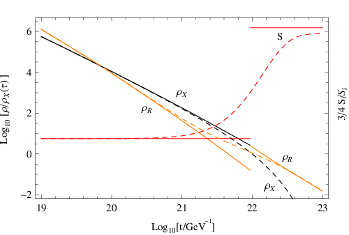
As an example, in Fig. 1 (dashed lines) the numerical evolution of $\rho_{R}(t)$ , $\rho_{X}(t)$ and $S(t)$ in the Standard Model (SM) are shown for initial conditions $\rho_{R}^{i}/\rho_{X}^{i}=10^{10},T_{i}=10^{9}$ GeV and $\tau=10^{22}$ GeV^-1. The corresponding dilution factor turns out to be $\Delta\simeq 7.8$ .

Refer to caption — Figure 1: Evolution of the energy densities $\rho_{R}$ and $\rho_{X}$ and the total entropy $S$ as function of time for initial conditions $\rho_{R}^{i}/\rho_{X}^{i}=10^{10},T_{i}=10^{9}$ GeV and $\tau=10^{22}$ GeV^-1. The result of the numerical (analytical) solution is shown by dashed (solid) lines. The $X$ -dominated epoch starts at $t_{e}$ and finishes at $t_{d}$ .

II.2 Analytic approximation

A straightforward analytic approximation to estimate the entropy dilution $\Delta$ is based on simplifying the previous exponential decay to an instantaneous one occurring at the time $t_{d}\simeq\tau$ [14] ³³ 3 The present fully-analytic approach is the most straightforward for practical purposes, so we will compare our numerical results with it. For some semi-analytic approximations see Ref. [15].. This approximation implies $S(t)=S_{i}$ for $t<t_{d}$ and it yields an evolution of the Universe as the one described by solid lines in Fig. 1, as we prove now.

Let us assume the Universe to be radiation dominated at the initial time $t_{i}$ ⁴⁴ 4 In practice other reliable situations can be led to this case by shifting and redefining the time.. For large enough $\tau$ there exists an equilibrium time $t_{e}$ ( $\gg t_{i}$ ) after which $\rho_{R}$ becomes smaller than $\rho_{X}$ . Using $S_{i}=S_{e}$ (quantities with the index $i,e,d,rh$ are evaluated at $t=t_{i},t_{e},t_{d}^{-},t_{d}^{+}$ , respectively) one gets

\rho_{R}^{e}=\rho_{X}^{e}=\frac{g_{e}T_{e}^{3}}{g_{i}T_{i}^{3}}\rho_{X}^{i}\quad\Rightarrow\quad T_{e}=T_{i}\rho_{X}^{i}/\rho_{R}^{i}~.

(9)

By taking the total energy and the scale factor $R$ to be constant at the moment of the decay, it turns out to be

\rho^{d}_{X}\equiv\rho_{X}(t_{d}^{-})=\rho^{rh}_{R}\equiv\rho_{R}(t_{d}^{+})~,

(10)

and subsequently

\rho_{R}^{rh}=\frac{g_{d}T_{d}^{3}}{g_{e}T_{e}^{3}}\rho_{R}^{e}\quad\Rightarrow\quad T_{rh}^{4}=\frac{g_{d}}{g_{rh}}T_{d}^{3}T_{e}~,

(11)

which implies an (apparent) instantaneous growth of $T$ ⁵⁵ 5 Alternatively, the instantaneous decay could be treated by maintaining fixed $T$ and increasing instantaneously $R$ . This would not lead to different conclusions..

The time $t_{d}$ , at which the sudden decay produces the discontinuity, is related to $\tau$ by the definition

\frac{3}{2}H[\rho_{X}^{d}]\equiv\tau^{-1}~,

(12)

where the chosen prefactor $3/2$ is motivated by the matter-like dominated epoch prior to the decay. Correspondingly, at $t=t_{d}$ the $X$ decay increases the entropy by the factor

\Delta=\frac{S_{rh}}{S_{d}}=\frac{g_{rh}T_{rh}^{3}}{g_{d}T_{d}^{3}}=\frac{T_{e}}{T_{rh}}~,

(13)

and, since Eqs. (10) and (12) imply

T_{rh}^{4}=\frac{40~m_{P}^{2}}{\pi^{2}g_{rh}\tau^{2}}~,

(14)

one concludes

\Delta=1.38\times 10^{-9}~\frac{\rho_{X}^{i}}{T_{i}^{3}}~\frac{g_{rh}^{1/4}}{g_{i}}~\left(\frac{\tau}{{\rm\ GeV}^{-1}}\right)^{1/2}~.

(15)

In the rest of the paper we will use Eqs. (14) and (15) as analytic estimates of the re-reheating temperature and entropy dilution.

Notice that Eq. (13) and thus (15) are strongly sensitive to the evaluation of $T_{e}$ which derives from the equality $S_{i}\!=\!S_{e}$ that is valid only for $t_{e}\!\ll\!\tau$ . Hence for $\Delta\approx 1$ , i.e. $T_{e}\simeq T_{rh}$ , Eq. (15) is unreliable. On the other hand, Eq. (15) turns out to be realistic for $\Delta\gg 1$ , as Fig. 1 suggests and as we will show in the next section.

Fig. 1 also highlights that the sudden decay approximation is not useful to describe quantities at $t\lesssim\tau$ at which the discrepancy with the numerical quantities is huge. In particular, it is well known that the discontinuity of $T$ at $t=t_{d}$ is an artifact of the crude approximation: actually the temperature of the Universe always decreases smoothly during the decay [15], as the numerical analysis in Fig. 1 highlights.

Finally, notice that in order to compare the evolutions of the analytical and numerical quantities in Fig. 1, the different scale factors $R(t)$ relative to each one of the two approaches are introduced. This allows to observe that in the numerical evolution $\rho_{X}$ returns subdominant near $t=\tau$ , what is reproduced in the analytic approximation thanks to the factor 3/2 chosen in the definition (12). If this factor were lowered, the instant of the temperature discontinuity would be anticipated.

II.3 Entropy production and re-reheating temperature

Besides the entropy dilution, the estimates of the re-reheating temperature $T_{rh}$ obtained by the analytic and numerical approaches are important. However, while in the sudden decay approximation $T_{rh}$ is well defined – it is the temperature just after the decay – in the numerical method it is not. In order to extend the concept of re-reheating temperature to the latter case we introduce the convention considering that the entropy injection ends when its remaining variation $\xi$ is tiny. In this way in the numerical analysis we can define implicitly $T_{rh}$ as $S(T\ll T_{rh})/S(T_{rh})\equiv 1+\xi$ and, after an opportune choice of $\xi$ , we can use the bound

T_{rh}\geq T_{BBN}~,

(16)

to avoid alterations of BBN predictions.

To determine $\xi$ we observe that 1% of entropy injection after $T_{BBN}$ roughly corresponds to the resolution of the measurements (1) and (2). This means that even in the pathological parameter scenario yielding $Y_{B}(T=T_{BBN})\simeq 8.4\times 10^{-11}$ [the lower bound allowed by (1) and (2)], a further 1% dilution does not lower appreciably $Y_{B}$ which then remains within the experimental constraint at any $T\leq T_{BBN}$ . For this reason, the requirement of not jeopardizing the BBN predictions can be safely replaced by the bound (16) with $\xi=0.01$ (see Appendix for considerations about other choices of $\xi$ ). Consequently, the definition of reheating temperature that we will use in the numerical analysis will be

\frac{S(T\ll T_{rh})}{S(T_{rh})}\equiv 1.01~.

(17)

II.4 Analytical versus numerical

In Fig. 2 we show the numerical (solid) and analytical (dashed) contour lines of $\Delta$ as function of $\tau$ and $\rho_{X}^{i}/T_{i}^{3}$ . The analytical lines are produced with $g(T)=106.75$ for simplicity while the numerical curves are calculated with the exact $g(T)$ of the SM [14]. As expected from Eq. (15), once $T_{i}$ is high enough to guarantee the initial radiation-dominated epoch, $\Delta$ is basically independent of it for $\rho_{X}^{i}/T_{i}^{3}$ and $g_{i}$ fixed.

We also determine numerically the parameter space violating the BBN bound (16). This region corresponds to the filled area of Fig. 2, whose border curve $T_{rh}=T_{BBN}$ reaches the line $\Delta=1.01$ asymptotically. This constraint on $\tau$ is by one order of magnitude stronger than the one obtained analytically by Eq. (14).

The numerical analysis highlights the existence of small entropy dilution even in absence of a $X$ -dominated epoch. Indeed below the dotted-dotted-dashed line of Fig. 2 the $X$ field decays before $\rho_{X}$ reaches $\rho_{R}$ but produces anyway a dilution $\Delta\lesssim 2.8$ . Approaching this regime corresponds to considering $t_{e}\simeq\tau$ for which the analytic approximation fails, as we already have stated in Section II.2. As a consequence, the constraint $\Delta<1.01$ evaluated analytically allows for values of $\rho_{X}^{i}/T_{i}^{3}$ that actually are excluded by two order of magnitude. Instead for $\Delta=10,10^{2},10^{5},10^{8},10^{10}$ the analytical and numerical curves are in good agreement and the difference appearing at large $\tau$ is due to the simplification $g(t)=106.75$ in the analytic estimates.

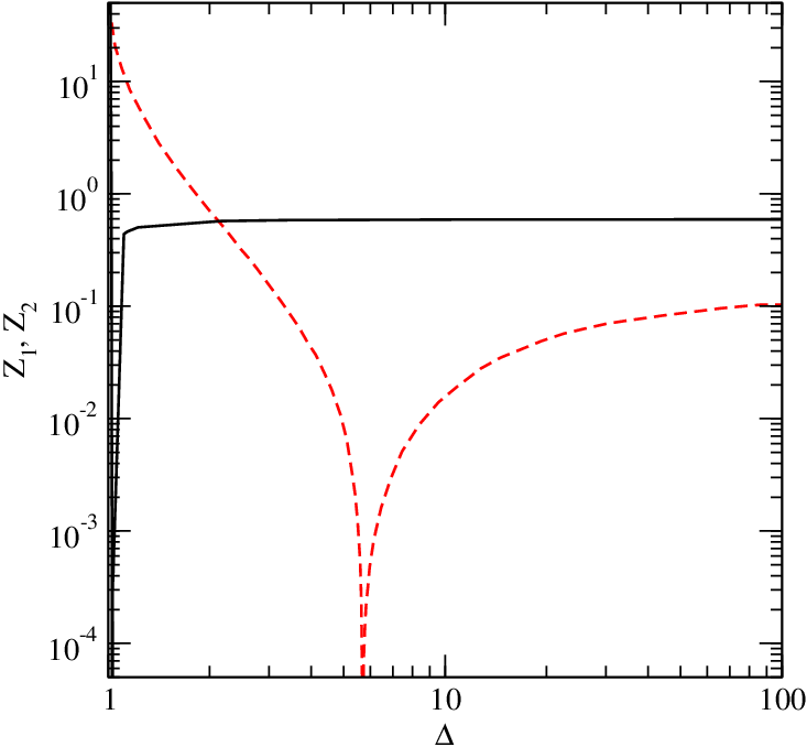
At this point one might be interested in knowing by what factors one should correct the analytic results in order to reproduce the numerical outcomes. These factors can be extracted from Fig. 3 where the absolute percentage errors

Z_{1}\equiv|T_{rh}^{(num)}/T_{rh}^{(ana)}-1|~,

Z_{2}\equiv|(\rho_{X}^{i}/T_{i}^{3})^{(ana)}/(\rho_{X}^{i}/T_{i}^{3})^{(num)}-1|~,

are plotted as function of $\Delta$ (at $\tau=10^{14}\,{\rm GeV}^{-1}$ but $Z_{1}$ and $Z_{2}$ are essentially independent of $\tau$ ). It turns out that the analytic approach overestimates $T_{rh}$ by a factor $\beta\simeq 2.5$ , typically. Moreover for a given value of $\rho_{X}^{i}/T_{i}^{3}$ , it underestimates the entropy dilution when $\Delta\lesssim 6$ and its error remains below $\sim 10\%$ when $\Delta\gtrsim 3$ . In particular, the error in estimating the dilution by Eq. (13) or (15) cannot be attributed univocally to a mismatch in $T_{rh}$ [which might be due to a wrong choice of the prefactor in Eq. (12)] because in such a case the equality $Z_{1}=Z_{2}$ should always arise ( $T_{e}$ is evaluated very precisely in both approaches for $\Delta\gg 1$ ).

III Baryogenesis bounds

The formation of primordial elements requires $Y_{B}(t)$ at BBN times to be compatible with the measures (1) and (2). In the previous section we used these bounds to constrain the history of $S(t)$ by assuming $N_{B}(t)$ constant at $T\lesssim T_{BBN}$ . However, further constraints on the $X$ decay can be inferred by knowing the evolution of $N_{B}(t)$ before BBN, as we explain now.

Let us consider a given baryogenesis mechanism that at the temperature $T_{B}$ generates a $B$ asymmetry $Y_{B}^{max}$ at best. Depending on the relative times at which the $B$ asymmetry and entropy dilution are produced, three different cases are possible:

1.

the entropy injection occurs exclusively after $T_{B}$ and thus the condition $\Delta\leq Y_{B}^{max}/Y_{B}^{exp}$ is required;
2.

the entropy injection happens exclusively before $T_{B}$ (i.e., $T_{rh}>T_{B}$ ) and then any $\Delta$ is allowed;
3.

the period of entropy injection encloses $T_{B}$ and hence the part of entropy produced after $T_{B}$ must be smaller than $Y_{B}^{max}/Y_{B}^{exp}$ ⁶⁶ 6 To avoid confusion in the definitions, we stress that $\Delta$ is the dilution due to the whole entropy produced by the $X$ decay, while $\tilde{\Delta}$ is only that portion of dilution occurring exclusively after $T_{B}$ .:

$\tilde{\Delta}(T_{B})\equiv\frac{S(T\ll T_{rh})}{S(T_{B})}\leq Y_{B}^{max}/Y_{B}^{exp}~.$ (18)

Notice that the parameter space fulfilling Eq. (18) includes the region contemplated by the possibilities 1 and 2. Therefore the parameter region where a given baryogenesis mechanism is compatible with the $X$ decay is determined by the bound (18).

As example, in Fig. 4 we present the $\tilde{\Delta}$ constraints (dotted lines) for some baryogenesis mechanisms generating $Y_{B}^{max}/Y_{B}^{exp}=10,10^{2},10^{5},10^{6}$ at $T_{B}=10^{5}$ (the figure also reports the numerical lines $\Delta=10,10^{2},10^{5},10^{6}$ in solid). The parameter space excluded by each $\tilde{\Delta}$ bound stands on the right of the corresponding line ⁷⁷ 7 In realistic cases $T_{B}$ stands for the temperature interval during which the $B$ asymmetry is created. Here we work in the limit that the entropy produced during this interval is negligible. On the contrary, the vertical part of the $\tilde{\Delta}$ curves is stumped while its oblique section holds sharp..

The curves $\tilde{\Delta}$ and $\Delta$ overlap asymptotically because at large $\tau$ the entropy is injected mostly after $T_{B}$ and hence we have $S(T_{B})\simeq S(T_{i})$ in Eqs. (8) and (18). Thus, in this regime the parameter space excluded by Eq. (18) can be derived analytically by the condition $\Delta\leq Y_{B}^{max}/Y_{B}^{exp}$ .

Instead, in the region where the curves $\tilde{\Delta}$ are vertical there is no bound on $\Delta$ but only on $\tau$ . In such a region the $\tilde{\Delta}$ condition is much less stringent than naively requiring $T_{rh}\geq T_{B}$ (which actually corresponds to $\tilde{\Delta}\simeq 1$ ). The reason is that big values of $Y_{B}^{max}/Y_{B}^{exp}$ allow for large dilutions of the produced $B$ asymmetry so that a region with $T_{rh}<T_{B}$ is permitted. This is quantified in Table I where for various values of $Y_{B}^{max}/Y_{B}^{exp}$ we report the bounds on $t_{B}/\tau$ and $T_{B}/T_{rh}$ valid in the regime of very large $\Delta$ , that is, when the curve $\tilde{\Delta}$ is vertical.

The interesting issue is that the values in Table I are basically independent of variation on $t_{B}$ and $T_{B}$ . Moreover the shape of the curves of the bounds $\tilde{\Delta}$ is universal, as we see in Fig. 4 where every dotted line could be obtained by the translation of one of the others. This implies that by our results anyone can take some long–lived field and baryogenesis mechanism and determine their compatibility without implementing further numerical analyses. To do it, one needs only to locate the curve (18) in the plan $\tau$ – $\rho_{X}^{i}/T_{i}^{3}\,$ for the desired framework. This can be achieved as follows.

$\tilde{\Delta}<$	$10$	$10^{2}$	$10^{3}$	$10^{4}$	$10^{5}$	$10^{6}$
$t_{B}/\tau\gtrsim$	$2\hskip-1.42262pt\times\hskip-1.42262pt10^{-1}$	$3\hskip-1.42262pt\times\hskip-1.42262pt10^{-2}$	$5\hskip-1.42262pt\times\hskip-1.42262pt10^{-3}$	$7\hskip-1.42262pt\times\hskip-1.42262pt10^{-4}$	$1\hskip-1.42262pt\times\hskip-1.42262pt10^{-4}$	$2\hskip-1.42262pt\times\hskip-1.42262pt10^{-5}$
$T_{B}/T_{rh}\hskip-1.42262pt\lesssim$	$3.4$	$5.5$	$8.8$	$14$	$21$	$33$

Table 1: Numerical evolution of the bound on

\tau

(

T_{rh}

) as function of

\tilde{\Delta}

and

t_{B}

(

T_{B}

) in the regime of very large

\Delta

First of all, one has to obtain the horizontal position of the $\tilde{\Delta}$ curve. This is provided by the constraint on $\tau$ in presence of very large $\Delta$ (namely, the position of the vertical part of the $\tilde{\Delta}$ curve). It can be found by Eq. (14) relating $\tau$ to the analytic estimate of $T_{rh}$ which in turn is constrained by

T_{rh}\gtrsim\frac{\beta}{\gamma}T_{B}\qquad({\rm for~large~}\Delta)~.

(19)

In this expression $\gamma$ is the opportune value in the second row of Table I connecting $T_{B}$ to the numerical estimate of $T_{rh}$ , while $\beta\simeq 2.5$ is the corrective factor at large $\Delta$ determined in Section II.4. Subsequently, the horizontal position of the $\tilde{\Delta}$ curve is given by

\tau\lesssim 7.7\times 10^{17}{\rm\ GeV}\frac{\gamma^{2}}{T_{B}^{2}\sqrt{g_{rh}}}\qquad({\rm for~large~}\Delta)~.

(20)

Afterwards, one needs to fix the vertical position of the $\tilde{\Delta}$ curve. This is furnished by Fig. 2 because for $\tau\rightarrow\infty$ we have

\tilde{\Delta}\approx\Delta\leq Y_{B}^{max}/Y_{B}^{exp}\qquad({\rm for~large~}\tau)~.

(21)

In conclusion, the compatibility of late-time entropy injection with successful baryogenesis can be calculated by using simple arithmetic. Some concrete examples will clarify how this procedure can be applied in realistic scenarios.

IV Explicit Applications

The procedure we have just presented is model independent except but the assumptions:

i)

the $X$ decay follows Eq. (3), does not induce a $B$ asymmetry and its products thermalize fast.

Moreover it is opportune to have:

ii)

the BAU production is much faster than the entropy injection.

Therefore, the described procedure allows for investigating the compatibility between any specific baryogenesis mechanism and any particular $X$ field satisfying the conditions i and (possibly) ii. As explicit applications, we will analyze some concrete mechanisms embedded in the MSSM whose $g(T)$ is calculated taking the scalar [fermion] content at $\mathcal{O}(1)$ [ $\mathcal{O}(0.1)$ ] TeV for definiteness.

IV.1 Some baryogenesis mechanisms

Here we apply our results to electroweak baryogenesis and thermal (resonant and non resonant) leptogenesis in presence of a generic $X$ field. For each baryogenesis framework we first review the estimate of $Y_{B}^{max}$ ⁸⁸ 8 We take the estimates of the literature assuming standard cosmology but in principle the evaluation of $Y_{B}^{max}$ could change when the BAU is produced in the $X$ -dominated era. However, for our concrete baryogenesis examples, Refs. [16, 17] find small modifications of $Y_{B}^{max}$ and $T_{B}$ so that we can use the standard results. and then we calculate the parameter region where the $X$ field does not destroy the BAU. The results will be summarized in Fig. 5, in which also the BBN bound and some $\Delta$ contour (dotted dashed) curves for the MSSM are reported.

IV.1.1 Electroweak Baryogenesis

In electroweak baryogenesis the observed BAU is produced during the electroweak symmetry breaking [18]. In this scenario the departure from thermal equilibrium is achieved by a first order electroweak phase transition (EWPT). In such a case the transition proceeds via nucleation of bubbles containing the electroweak broken phase and the movement of the bubble breaks locally the thermal equilibrium conditions. Then, just in front of the expanding bubbles, $C$ and $CP$ violating interactions generate a left-handed asymmetry that $SU(2)_{L}$ sphalerons transform to a $B$ asymmetry entering the bubble. However, the formation of the $B$ asymmetry is not enough: it is also necessary to preserve it till today. This occurs if the first order EWPT is strong ⁹⁹ 9 The EWPT is strong when $SU(2)_{L}$ sphalerons are out-of-equilibrium inside the bubbles. Unless of subtle circumstances [17, 19] not considered here, this happens for $v(T_{B})/T_{B}\gtrsim 0.7$ where $v\equiv v(T=0)=174\,{\rm\ GeV}$ and $v(T_{B})$ is the vacuum expectation value of the (SM-like) Higgs at the temperature $T_{B}$ when the phase transition begins [18]..

In the SM the EWPT is not strong and the $CP$ violating sources are too small to form enough $B$ asymmetry [18]. These problems are overcome in some extensions of the SM. Some non-supersymmetric scenarios have been considered [20] but at present the analyses of them are not so developed to provide precise estimates of the maximal $B$ asymmetry these models can produce. Instead accurate predictions exist for supersymmetric extensions.

The MSSM can reproduce the observed BAU if the gaugino-Higgsino sector is at the electroweak scale [21, 22, 23, 24, 25], the SM-like Higgs and right-handed stop are light ( $m_{h}\lesssim 127$ GeV, $m_{\tilde{t}_{R}}\lesssim 120$ GeV) and the left-handed stop is heavy ( $m_{\tilde{t}_{L}}\gtrsim 6.5$ TeV) [26]. Moreover, the $B$ asymmetry formation typically starts at $T_{B}\simeq 125$ GeV and ends after a few GeV [26]. Finally, concerning $Y_{B}^{max}$ , different treatments of $CP$ -violating sources and flavor effects exist [23, 24, 25] and they lead to $B$ asymmetries that may differ by almost one order of magnitude. Choosing the intermediate result we can consider $Y_{B}^{max}\simeq 10\,Y_{B}^{exp}$ [23, 26].

In conclusion, the parameter space where electroweak baryogenesis in the MSSM is compatible with the $X$ decay is given by the constraint

\tilde{\Delta}(T_{B}\simeq 125{{\rm\ GeV}})\lesssim 10~,

(22)

in which the condition ii is fulfilled because the $B$ asymmetry is produced in a narrow temperature interval ${\mathcal{O}}(1{\rm\ GeV})$ .

The numerical solution of Eq. (22) gives the area labelled EWBG in Fig. 5. Its border curve could be calculated by the analytic procedure expressed in Section III. In fact, the position of the vertical part of the curve is given by Eq. (20) yielding $\tau\lesssim 5\hskip-1.42262pt\times\hskip-1.42262pt10^{13}{\rm\ GeV}^{-1}$ for $g_{rh}=g(T_{rh}=92{\rm\ GeV})\simeq 100$ and $\gamma=3.4$ , while at much larger $\tau$ the line must coincide with the bound $\Delta<10$ because of Eq. (21). Instead, in the intermediate regime of $\tau$ the curve is deduced by the universal shape of the $\tilde{\Delta}$ lines of Fig. 4.

Before concluding, some words about electroweak baryogenesis in non-minimal supersymmetric extensions are in order. The estimate $Y_{B}^{max}\hskip-2.84526pt\approx\hskip-2.84526pt10Y_{B}^{exp}$ holds roughly correct also in extensions of the MSSM where the extra content couples weakly to the Higgs sector and no new large sources of $CP$ violation are introduced. This is not the case if an extra singlet is added to the MSSM as it is performed in Ref. [27]. In such a extension $Y_{B}^{max}$ can be enhanced approximatively by a factor 5. Moreover, other modifications of the minimal setup can further enhance $Y_{B}^{max}$ , as for instance in the extension called Beyond-the-MSSM where $Y_{B}^{max}$ may increase by a further order of magnitude [28]. Here we do not explicitly repeat the analysis for all these variations but their compatibility with a late-time entropy injection could be easily figured out algebraically as we have just performed for the MSSM.

IV.1.2 Thermal Leptogenesis

Leptogenesis is one of the attractive scenarios to explain the BAU [29, 30]. Its central idea is that in a $B$ -symmetric but Lepton( $L$ )-asymmetric Universe it is possible to produce the BAU thanks to electroweak sphalerons that equilibrate the $B$ + $L$ asymmetry without changing $B$ – $L$ . In thermal leptogenesis the required initial $L$ asymmetry can be obtained for instance in the Type-I seesaw framework [31] where one singlet right-handed neutrino $N$ per family is added to the SM ¹⁰¹⁰ 10 Our conclusions do not change for Type-II and Type-III [32].. These fields have the interactions

\mathcal{L}\supset\frac{1}{2}(M_{N})_{ii}N_{i}N_{i}+y_{ij}N_{i}\bar{\ell}_{j}i\tau_{2}H^{*}+{\rm h.c.}\;,

(23)

in which $l$ ( $H$ ) is the SM lepton (Higgs) and indeces run over families. They not only give rise to a net $L$ asymmetry in the early Universe by out-of-equilibrium decays but also generate sub-eV neutrino masses via the canonical seesaw mechanism as required by the neutrino oscillation data [33]. This mass turns out to be $m_{\nu}\approx|y|^{2}v^{2}/M_{N}$ yielding $M_{N}\sim 10^{14}$ GeV for $|y|\sim 1$ and $m_{\nu}\sim 0.1{\rm\ eV}$ .

Assuming a normal hierarchy in the heavy neutrino sector, the $CP$ asymmetry of the decay of the lightest right-handed neutrino $N_{1}$ is given by [34]

|\epsilon^{I}|=\frac{3M_{N_{1}}}{16\pi v^{2}}\sqrt{\Delta m^{2}_{\rm atm}}~\sin\delta~,

(24)

where $\Delta m^{2}_{\rm atm}$ is the atmospheric mass scale of light neutrinos [33] and $\delta$ is the effective $CP$ violating phase.

The $L$ asymmetry, which is mostly produced by the decay of $N_{1}$ , is given by $Y_{L}=\epsilon^{I}Y_{N_{1}}W$ where the thermal wash out $W$ takes into account the effect of interactions reducing the created $L$ asymmetry, as for instance $\bar{l}H\leftrightarrow lH^{*}$ . Afterwards, electroweak sphalerons tend to equilibrate the $B$ + $L$ asymmetry and so they convert around half part of $Y_{L}$ into $Y_{B}$ . Therefore, in order to determine the maximal $B$ asymmetry $Y_{B}^{max}$ , one sets $\sin\delta=1$ and obtains [34]

\frac{Y_{B}^{max}}{Y_{B}^{exp}}\approx 4\times 10^{4}\left(\frac{M_{N_{1}}}{10^{14}\rm GeV}\right)\frac{\sqrt{\Delta m^{2}_{\rm atm}}}{0.05\rm eV}\left(\frac{Y_{N_{1}}W}{7\times 10^{-4}}\right)~.

Since commonly the framework is supposed to be embedded in a grand unified theory and moreover the Universe typically never reached temperatures high enough to thermally generate neutrinos beyond the GUT scale, we can consider $10^{16}\gtrsim M_{N_{1}}\hskip-2.84526pt{\rm\ GeV}^{-1}\gtrsim 10^{9}$ , where the lower bound comes from requiring enough BAU in Eq. (IV.1.2).

Now we can analyze the $B$ -asymmetry dilution due to $X$ decay ¹¹¹¹ 11 An analysis focused on solving the gravitino problem in a particular framework of thermal leptogenesis and late-time decay is presented in Ref. [9].. Taking $T_{B}\approx M_{N_{1}}$ , the case $M_{N_{1}}\simeq 10^{9}{\rm\ GeV}$ gives $Y_{B}^{max}/Y_{B}^{exp}=\mathcal{O}(1)$ and yields then

\tilde{\Delta}(T_{B}\simeq 10^{9}{\rm\ GeV})\lesssim{\cal O}(1)~.

(25)

Eq. (25) permits any $\Delta$ for $\tau\lesssim 10^{-1}{\rm\ GeV}^{-1}$ but does not provide a sharp bound on $\tau$ because the condition ii is not guaranteed. Similarly for $M_{N_{1}}\simeq 10^{16}{\rm\ GeV}$ , which yields $Y_{B}^{max}/Y_{B}^{exp}=\mathcal{O}(10^{6})$ , we have the constraint

\tilde{\Delta}(T_{B}\simeq 10^{16}{\rm\ GeV})\lesssim{\cal O}(10^{6})~,

(26)

that allows any dilution $\Delta\lesssim 10^{6}$ independently of $\tau$ .

The union of the regions fulfilling (25) and (26) gives the parameter space where thermal leptogenesis is compatible with the $X$ decay. The numerical result is shown in Fig. 5 (green area labelled TLP) and could be reproduced algebraically by the procedure explained in Section III and already applied for electroweak baryogenesis.

IV.1.3 Resonant thermal leptogenesis

The $CP$ asymmetry in Eq. (24) requires very heavy additional neutrinos to produce the BAU. For this reason thermal leptogenesis with normal neutrino hierarchy provides no experimental evidence at current achievable energies. This unappealing feature is avoided in resonant thermal leptogenesis where extra neutrinos at the electroweak scale may yield BAU and detectable signatures at the same breath [35].

The key idea of resonant leptogenesis [36, 37] is that the self-energy effects dominate the leptonic asymmetries when the mass splitting between the right-handed neutrinos $N$ is much less than their masses. If the mass splitting between these fields is comparable to their decay widths, the $CP$ asymmetry gets enhanced resonantly.

Focusing on type-I leptogenesis (our conclusions would not change for type II and III), let us consider two singlet Majorana fields $N_{1}$ and $N_{2}$ of masses $M_{1}$ and $M_{2}$ . Their Yukawa interaction $h_{ij}N_{i}\bar{\ell}_{j}H$ allows for decays to SM lepton $\ell$ and Higgs doublet H whose $CP$ asymmetry is given by [38]

\epsilon_{1}=\frac{{\rm Im}(h^{\dagger}h)_{12}^{2}}{8\pi(h^{\dagger}h)_{11}}\frac{(M_{1}^{2}-M_{2}^{2})M_{1}M_{2}}{(M_{1}^{2}-M_{2}^{2})^{2}+(M_{2}\Gamma_{2}-M_{1}\Gamma_{1})^{2}}~.

(27)

Hence, assuming $M_{1}\sim M_{2}$ and $M_{1}-M_{2}\sim\Gamma_{1}-\Gamma_{2}$ we can achieve $\epsilon_{1}\sim{\cal O}(1)$ so that a large $L$ asymmetry $Y_{L}$ can be produced even if the initial $N_{1}$ and $N_{2}$ abundance $Y_{N}$ is small. Finally, $SU(2)_{L}$ sphalerons can convert $Y_{L}$ to $Y_{B}$ if the lepton asymmetry is produced enough before $T\simeq 130\,$ GeV when sphalerons decouple [39]. Typically, this happens if $M_{1}\gtrsim 250{\rm\ GeV}$ [37]. In such a case it turns out $Y_{B}\simeq 0.5\times\epsilon_{1}Y_{N}W$ , where it is reasonable to consider $Y_{N}W=\mathcal{O}(10^{-4})$ [35] yielding $Y_{B}^{max}={\cal O}(10^{-4})$ for $\epsilon_{1}\sim{\cal O}(1)$ .

In conclusion, in resonant leptogenesis it turns out to be $Y_{B}^{max}\approx\mathcal{O}(10^{6})Y_{B}^{exp}$ . Moreover, in order to favor the compatibility with the late-time decay, $T_{B}$ has to be as low as possible. Since it is $T_{B}\approx M_{1}$ , the most favorable choice is $M_{1}\approx 250\,$ GeV. Subsequently, resonant leptogenesis is compatible with the $X$ decay when the constraint

\tilde{\Delta}(T_{B}\simeq 250{\rm\ GeV})\lesssim\mathcal{O}(10^{6})~,

(28)

is fulfilled. Observe that this constraint can be considered as a sharp bound since the condition ii is satisfied due to the short temperature interval during which the $B$ asymmetry is generated ( $250\!\gtrsim\!T\!/\!\!{\rm\ GeV}\!\gtrsim\!130$ ).

By solving Eq. (28) numerically, one finds that the excluded region is the area labelled RLPT shown in Fig. 5. As already checked for the previous baryogenesis mechanisms, the excluded region could be easily determined algebraically by the procedure of Section III. Indeed its vertical border is due to the bound $\tau\gtrsim 1\times 10^{15}{\rm\ GeV}^{-1}$ coming from Eq. (20) with $g_{rh}=g(T_{rh}=18{\rm\ GeV})\simeq 90$ and $\gamma=33$ , its lower part corresponds to the constraint $\tilde{\Delta}\simeq\Delta<10^{6}$ shown in Fig. 2, and the curved part is deduced by copying the shape of the $\tilde{\Delta}$ lines of Fig. 4.

IV.2 $X$ field as a modulus

In the examples we have just considered the field producing the late-time entropy is not specified. Now we analyze the particular case of the $X$ field being a modulus. Let us assume it to be gravitationally coupled to the SM thermal bath via a dimension-five operator so that its lifetime is given by

\tau=\frac{2\pi}{\alpha_{X}}\left(\frac{m_{P}^{2}}{M_{X}^{3}}\right)~,

(29)

where $\alpha_{X}$ spans from ${\cal O}(1)$ to ${\cal O}(10^{-2})$ depending on the non-renormalizable coupling [40].

In an expanding Universe, when the Hubble scale is roughly equal to the modulus mass, $H\approx M_{X}$ , the modulus enters into the oscillating regime. By taking the initial amplitude of oscillations of $X$ to be ${\mathcal{X}}_{i}$ , the energy density $\rho_{X}^{i}$ can be expressed as

\rho_{X}^{i}=M_{X}^{2}\mathcal{X}_{i}^{2}~.

(30)

Moreover, when the field starts oscillating, the Universe is radiation dominated and its temperature $T_{i}$ is

T_{i}^{4}=\frac{90~m_{P}^{2}M_{X}^{2}}{\pi^{2}g_{i}}~.

(31)

Subsequently, we can easily convert the model independent bounds of the previous sections to the case of $X$ as a modulus. For instance, the general bounds on $\tau$ and $\rho_{X}^{i}/T_{i}^{3}$ presented in Fig. 5 can be re-expressed as constraints on $\mathcal{X}_{i}$ and $M_{X}$ , as shown in Fig. 6.

Using Eqs. (29)-(31), the sudden decay approximations (9), (13) and (14) become

$\displaystyle T_{e}^{4}$	$\displaystyle=$	$\displaystyle\frac{10}{9\pi^{2}g_{i}}\frac{\mathcal{X}_{i}^{8}M_{X}^{2}}{m_{P}^{6}}~,$	(32)
$\displaystyle T_{rh}^{4}$	$\displaystyle=$	$\displaystyle\frac{10}{\pi^{4}g_{rh}}\frac{\alpha_{X}^{2}M_{X}^{6}}{m_{P}^{2}}~,$	(33)
$\displaystyle\Delta$	$\displaystyle=$	$\displaystyle\sqrt[4]{\frac{\pi^{2}~g_{rh}}{9~g_{i}}}\frac{\mathcal{X}_{i}^{2}}{\sqrt{\alpha_{X}}m_{P}M_{X}}~,$	(34)

and the BBN bound $T_{rh}\!\geq\!4{\rm\ MeV}$ is converted to

M_{X}\gtrsim 7\times 10^{4}~(1/\alpha_{X})^{1/3}{\rm GeV}\qquad({\rm analytic})~,

(35)

which is slightly weaker than the numerical one. However, the BBN bound is not the strongest constraint in the regime of large oscillations. In such a regime, to avoid the BAU wash out, we need $M_{\!X}\!\sqrt[3]{\alpha_{X}}>{\cal O}(10^{13})$ GeV for thermal leptogenesis, $M_{\!X}\!\sqrt[3]{\alpha_{X}}>{\cal O}(10^{8})$ GeV for electroweak baryogenesis and $M_{\!X}\!\sqrt[3]{\alpha_{X}}>{\cal O}(10^{7})$ GeV for resonant leptogenesis.

V Conclusions

There exist many theories beyond the standard model of particle physics that predict cosmologically long-lived fields. Even though the initial energy density of these fields may be many orders of magnitude less than the one of radiation, at later times they can dominate the expansion of the Universe and dump sizeable amount of entropy during their decay. Subsequently these fields dilute the pre-processed $B$ asymmetry and may alter the primordial element abundances.

In order to constrain the above theories, in this paper we analyzed the entropy and the subsequent re-reheating that a generic long-lived field $X$ produces. We solved the decay equations numerically and we checked their consistency with the analytic sudden-decay approximation. The result can be parameterized by lifetime and initial energy density of the $X$ field. We found that for small entropy dilution $\Delta$ the analytic approximation badly fails because in this regime there is no clear $X$ -dominated epoch. Instead for $\Delta\gtrsim 3$ the analytic and numerical calculations disagree by less than 10% in the entropy estimates but by a factor $\sim$ 2.5 in the evaluation of $T_{rh}$ , the temperature at the end of the dilution. However, the errors of the analytic approach can be overcome by applying some corrective factors which, among other effects, strength slightly the BBN upper bound on the $X$ lifetime.

The revised control on entropy dilution and re-reheating temperature allowed us for investigating the effect of the $X$ decay on the $B$ asymmetry. The analysis was carried out by assuming the mechanism producing the entropy injection to be independent of the one generating the BAU. The outcome is a set of conditions on the lifetime and initial energy density of $X$ as function of when and in what amount the BAU is produced. These conditions are quite generic so that they can be easily applied to determine the compatibility of baryogenesis and late-time decay described by a wide class of scenarios.

As illustrative examples, we applied our results to some concrete models. It turned out that successful MSSM electroweak baryogenesis, thermal leptogenesis and resonant leptogenesis put strong bounds on the initial abundances of $X$ fields with lifetime $\tau\gtrsim 5\times 10^{13},10^{-2},10^{15}\,{\rm\ GeV}^{-1}$ , respectively. Instead, for smaller values of $\tau$ the abundance is not constrained (see Fig. 5). Furthermore, if we take $X$ being modulus as explicit example of decaying field, the above constraints become bounds on the initial oscillation amplitude $\mathcal{X}_{i}$ , mass $M_{X}$ and gravitationally-mediated coupling $\alpha_{X}$ to the visible sector. In particular, very large $\mathcal{X}_{i}$ implies excessive dilution of the $B$ asymmetry produced by MSSM electroweak baryogenesis, thermal leptogenesis and thermal resonant leptogenesis for $M_{\!X}\!\sqrt[3]{\alpha_{X}}\gtrsim 10^{8},10^{13},10^{7}\,{\rm\ GeV}$ , respectively (see Fig. 6).

Acknowledgements.

We are grateful to A. Mazumdar for inspiring discussions and suggestions in several stages of the paper. We also thank T. Hambye and C. Ringeval for comments on the manuscript and on CMB bounds. G.N. thanks M. Carena, T. Konstandin, M. Quirós and C. Wagner for many discussions on electroweak baryogenesis. The work of G.N. and N.S. is supported by IISN and the Belgian Science Policy (IAP VI-11).

Appendix: Relaxing the BBN bound

Apart from some special exceptions [7], the observed primordial element abundances cannot be explained when sizeable entropy injections occur during the BBN epoch. On the contrary, the success of the standard BBN model is not spoiled for [6]

T_{rh}\geq T_{BBN}\equiv 4\,{\rm\ MeV}~,

(36)

where the $X$ -decay hadronic channels are supposed suppressed.

In our numerical analysis we implement the reheating temperature as

\frac{S(T\ll T_{rh})}{S(T_{rh})}\equiv 1+\xi~,

(37)

with $\xi=0.01$ . Subsequently $T_{rh}$ is the temperature of the thermal bath when the 99% of the entropy due to the $X$ decay has been injected.

Applying the definition (37) in the constraint (36) is consistent with BBN. Indeed, even in the pathological combination of baryogenesis and entropy mechanisms leading to $T_{rh}=T_{BBN}$ and $Y_{B}(T_{BBN})\simeq 8.4\times 10^{-11}$ [the minimal value allowed by Eqs. (1) and (2)], the remaining 1% of entropy injection after $T_{BBN}$ dilutes $Y_{B}$ by an amount that is practically negligible for the experimental constraints.

However, the convention $\xi=0.01$ is often too conservative. For instance, in the case with $T_{rh}=T_{BBN}$ and $Y_{B}(T_{BBN})\simeq 9.2\times 10^{-11}$ , the maximal allowed entropy dilution after $T_{BBN}$ is the ratio between the upper and lower bounds of $Y_{B}^{exp}$ . In such a case, by taking the allowed extrema of (1) and (2), the BBN bound can be implemented by (36) where $T_{rh}$ is redefined through (37) with $\xi=0.10$ . On the other hand, if possible systematic errors due to priors were taken into account in the WMAP analysis, the experimental bound (2) would be comparable with (1) [12] and the BBN bound could be further relaxed by redefining $T_{rh}$ by (37) with $\xi=0.27$ .

As a consequence, these different choices of $\xi$ slightly relax the BBN bound shown in the figures of the paper. For instance, the convention $\xi=0.27$ weakens the BBN constraint on $\rho_{X}^{i}/T_{i}^{3}$ (on $\tau$ ) by a factor $\sim$ 10 $(\sim$ 3). In any case for the possible values $0.01<\xi<0.27$ the numerical analysis still provides a BBN bound that is stronger than the one obtained analytically by Eq. (14).

References

[1] T. Gherghetta, C. F. Kolda, S. P. Martin, Nucl. Phys. B468 (1996) 37-58; K. Enqvist, A. Mazumdar, Phys. Rept. 380 (2003) 99-234.
[2] See for example, S. Kasuya, F. Takahashi, JCAP 0711 (2007) 019 and the references therein.
[3] See for example, B. Dutta, L. Leblond, K. Sinha, Phys. Rev. D80 (2009) 035014 and the references therein.
[4] See for example, K. Y. Choi, J. E. Kim, H. M. Lee and O. Seto, Phys. Rev. D 77 (2008) 123501 and the references therein.
[5] G. D. Coughlan, W. Fischler, E. W. Kolb, S. Raby and G. G. Ross, Phys. Lett. B 131 (1983) 59; B. de Carlos, J. A. Casas, F. Quevedo and E. Roulet, Phys. Lett. B 318 (1993) 447; T. Banks, D. B. Kaplan and A. E. Nelson, Phys. Rev. D 49 (1994) 779; T. Nagano, M. Yamaguchi, Phys. Lett. B438 (1998) 267-272; K. Kohri, M. Yamaguchi, J. ’i. Yokoyama, Phys. Rev. D70 (2004) 043522; M. Endo, K. Hamaguchi and F. Takahashi, Phys. Rev. Lett. 96 (2006) 211301; S. Nakamura and M. Yamaguchi, Phys. Lett. B 638 (2006) 389; M. Dine, R. Kitano, A. Morisse and Y. Shirman, Phys. Rev. D 73 (2006) 123518; M. Endo, K. Hamaguchi and F. Takahashi, Phys. Rev. D 74 (2006) 023531.
[6] M. Kawasaki, K. Kohri and N. Sugiyama, Phys. Rev. D 62 (2000) 023506; G. F. Giudice, E. W. Kolb, A. Riotto, D. V. Semikoz and I. I. Tkachev, Phys. Rev. D 64 (2001) 043512; S. Hannestad, Phys. Rev. D 70 (2004) 043506.
[7] K. Jedamzik, M. Pospelov, New J. Phys. 11 (2009) 105028 and references therein.
[8] T. Moroi and L. Randall, Nucl. Phys. B 570 (2000) 455; J. McDonald, Phys. Lett. B 511 (2001) 1; M. Nagai and K. Nakayama, Phys. Rev. D 76 (2007) 123501; K. Kohri, A. Mazumdar and N. Sahu, Phys. Rev. D 80 (2009) 103504; K. Kohri, A. Mazumdar, N. Sahu and P. Stephens, Phys. Rev. D 80 (2009) 061302; K. Hamaguchi, R. Kitano and F. Takahashi, JHEP 0909 (2009) 127; K. Kohri, J. McDonald and N. Sahu, Phys. Rev. D 81 (2010) 023530.
[9] J. Hasenkamp and J. Kersten, Phys. Rev. D 82 (2010) 115029.
[10] See for instance, G. Gelmini, P. Gondolo, A. Soldatenko and C. E. Yaguna, Phys. Rev. D 74 (2006) 083514.
[11] T. Moroi and T. Takahashi, Phys. Lett. B 522 (2001) 215 [Erratum-ibid. B 539 (2002) 303]; D. H. Lyth and D. Wands, Phys. Lett. B 524 (2002) 5; J. Martin, C. Ringeval and R. Trotta, Phys. Rev. D 83 (2010) 063524.
[12] K. Nakamura et al. [Particle Data Group (Chapter 20)], J. Phys. G 37 (2010) 075021;
[13] E. Komatsu et al. [WMAP Collaboration], Astrophys. J. Suppl. 192 (2011) 18.
[14] See for example: E. W. Kolb and M. S. Turner, Front. Phys. 69 (1990) 1.
[15] R. J. Scherrer and M. S. Turner, Phys. Rev. D31(1985)681.
[16] E. J. Chun and S. Scopel, JCAP 0710 (2007) 011.
[17] M. Joyce and T. Prokopec, Phys. Rev. D 57 (1998) 6022.
[18] See for example, M. Quiros, arXiv:hep-ph/9901312; J. M. Cline, arXiv:hep-ph/0609145.
[19] D. Comelli, D. Grasso, M. Pietroni and A. Riotto, Phys. Lett. B 458 (1999) 304; H. H. Patel and M. J. Ramsey-Musolf, JHEP 1107 (2011) 029; A. De Simone, G. Nardini, M. Quiros and A. Riotto, arXiv:1107.4317 [hep-ph]; G. Nardini and M. Quiros, work in progress.
[20] D. Bodeker, L. Fromme, S. J. Huber and M. Seniach, JHEP 0502 (2005) 026; J. Shu, T. M. P. Tait and C. E. M. Wagner, Phys. Rev. D 75 (2007) 063510; J. R. Espinosa and M. Quiros, Phys. Rev. D 76 (2007) 076004; S. Profumo, M. J. Ramsey-Musolf and G. Shaughnessy, JHEP 0708 (2007) 010; G. Nardini, M. Quiros and A. Wulzer, JHEP 0709 (2007) 077; J. R. Espinosa, T. Konstandin, J. M. No and M. Quiros, Phys. Rev. D 78 (2008) 123528; V. Barger, P. Langacker, M. McCaskey, M. Ramsey-Musolf and G. Shaughnessy, Phys. Rev. D 79 (2009) 015018; T. Konstandin, G. Nardini and M. Quiros, Phys. Rev. D 82 (2010) 083513; J. R. Espinosa, T. Konstandin and F. Riva, arXiv:1107.5441 [hep-ph].
[21] M. S. Carena, M. Quiros and C. E. M. Wagner, Phys. Lett. B 380 (1996) 81; D. Delepine, J. M. Gerard, R. Gonzalez Felipe and J. Weyers, Phys. Lett. B 386 (1996) 183; B. de Carlos and J. R. Espinosa, Nucl. Phys. B 503 (1997) 24; M. S. Carena, M. Quiros, A. Riotto, I. Vilja and C. E. M. Wagner, Nucl. Phys. B 503 (1997) 387; M. S. Carena, M. Quiros and C. E. M. Wagner, Nucl. Phys. B 524 (1998) 3.
[22] V. Cirigliano, Y. Li, S. Profumo and M. J. Ramsey-Musolf, JHEP 1001 (2010) 002.
[23] M. S. Carena, J. M. Moreno, M. Quiros, M. Seco and C. E. M. Wagner, Nucl. Phys. B 599 (2001) 158; M. S. Carena, M. Quiros, M. Seco and C. E. M. Wagner, Nucl. Phys. B 650 (2003) 24.
[24] C. Lee, V. Cirigliano and M. J. Ramsey-Musolf, Phys. Rev. D 71 (2005) 075010; V. Cirigliano, M. J. Ramsey-Musolf, S. Tulin and C. Lee, Phys. Rev. D 73 (2006) 115009; D. J. H. Chung, B. Garbrecht, M. J. Ramsey-Musolf and S. Tulin, Phys. Rev. Lett. 102 (2009) 061301; D. J. H. Chung, B. Garbrecht, M. J. Ramsey-Musolf and S. Tulin, JHEP 0912 (2009) 067; V. Cirigliano, C. Lee, M. J. Ramsey-Musolf and S. Tulin, Phys. Rev. D 81 (2010) 103503; V. Cirigliano, C. Lee and S. Tulin, arXiv:1106.0747 [hep-ph].
[25] T. Konstandin, T. Prokopec and M. G. Schmidt, Nucl. Phys. B 716 (2005) 373; T. Konstandin, T. Prokopec, M. G. Schmidt and M. Seco, Nucl. Phys. B 738 (2006) 1.
[26] M. Carena, G. Nardini, M. Quiros and C. E. M. Wagner, JHEP 0810 (2008) 062; Nucl. Phys. B 812 (2009) 243.
[27] A. Menon, D. E. Morrissey and C. E. M. Wagner, Phys. Rev. D 70 (2004) 035005; J. Kang, P. Langacker, T. j. Li and T. Liu, Phys. Rev. Lett. 94 (2005) 061801; S. J. Huber, T. Konstandin, T. Prokopec and M. G. Schmidt, Nucl. Phys. B757(2006)172; Nucl. Phys. A785(2007)206.
[28] K. Blum, C. Delaunay, M. Losada, Y. Nir and S. Tulin, JHEP 1005 (2010) 101.
[29] M. Fukugita and T. Yanagida, Phys. Lett. B174(1986)45.
[30] For a review see, W. Buchmuller, R. D. Peccei and T. Yanagida, Ann. Rev. Nucl. Part. Sci. 55 (2005) 311.
[31] P. Minkowski, Phys. Lett. B 67 (1977) 421; M. Gell-Mann, P. Ramond and R. Slansky in Supergravity (P. van Niewenhuizen and D. Freedman, eds), (Amsterdam), North Holland, 1979; T. Yanagida in Workshop on Unified Theory and Baryon number in the Universe (O. Sawada and A. Sugamoto, eds), (Japan), KEK 1979; R.N. Mohapatra and G. Senjanovic, Phys. Rev. Lett. 44 (1980) 912.
[32] T. Hambye and G. Senjanovic, Phys. Lett. B 582 (2004) 73; S. Antusch and S. F. King, Phys. Lett. B 597 (2004) 199; P. h. Gu and X. j. Bi, Phys. Rev. D 70 (2004) 063511; N. Sahu and S. Uma Sankar, Phys. Rev. D 71 (2005) 013006; N. Sahu and S. Uma Sankar, Nucl. Phys. B 724 (2005) 329; N. Sahu and U. Sarkar, Phys. Rev. D 74 (2006) 093002.
[33] M. C. Gonzalez-Garcia, M. Maltoni and J. Salvado, JHEP 1004 (2010) 056.
[34] W. Buchmuller, P. DiBari and M. Plumacher, Nucl. Phys. B 643 (2002) 367 [Erratum-ibid. B 793 (2008) 362]; S. Davidson and A. Ibarra, Phys. Lett. B 535 (2002) 25.
[35] R. Franceschini, T. Hambye and A. Strumia, Phys. Rev. D 78 (2008) 033002; S. Blanchet, T. Hambye and F. X. Josse-Michaux, JHEP 1004 (2010) 023.
[36] M. Flanz, E. A. Paschos and U. Sarkar, Phys. Lett. B 345 (1995) 248 [Erratum-ibid. B 382 (1996) 447]; M. Flanz, E. A. Paschos, U. Sarkar and J. Weiss, Phys. Lett. B 389 (1996) 693; L. Covi, E. Roulet and F. Vissani, Phys. Lett. B 384 (1996) 169.
[37] A. Pilaftsis, Phys. Rev. D 56 (1997) 5431; A. Pilaftsis and T. E. J. Underwood, Nucl. Phys. B 692 (2004) 303.
[38] W. Buchmuler and M. Plumacher, Phys. Lett. B 431 354 (1998); A. Anisimov, A. Broncano and M. Plumacher, Nucl. Phys. B 737 (2006) 176.
[39] Y. Burnier, M. Laine and M. Shaposhnikov, JCAP 0602 (2006) 007.
[40] See for example, R. Allahverdi, B. Dutta and K. Sinha, Phys. Rev. D D82 (2010) 035004.