Random Walk Picture of Basketball Scoring
Abstract
We present evidence, based on play-by-play data from all 6087 games from the 2006/07–2009/10 seasons of the National Basketball Association (NBA), that basketball scoring is well described by a continuous-time anti-persistent random walk. The time intervals between successive scoring events follows an exponential distribution, with essentially no memory between different scoring intervals. By including the heterogeneity of team strengths, we build a detailed computational random-walk model that accounts for a variety of statistical properties of scoring in basketball games, such as the distribution of the score difference between game opponents, the fraction of game time that one team is in the lead, the number of lead changes in each game, and the season win/loss records of each team.
1 Introduction
Sports provide a rich laboratory in which to study competitive behavior in a well-defined way. The goals of sports competitions are simple, the rules are well defined, and the results are easily quantifiable. With the recent availability of high-quality data for a broad range of performance metrics in many sports (see, for example, shrpsports.com), it is now possible to address questions about measurable aspects of sports competitions that were inaccessible only a few years ago. Accompanying this wealth of new data is a rapidly growing body of literature, both for scientific and lay audiences, on quantitative modeling and analysis of sports statistics (for general references, see, e.g., Mosteller (1997), Albert et al. (2005), Kubatko et al. (2007), Albert and Koning (2008), Glickman and Evans (2009), Arkes and Martinez (2011)).
In this spirit, our investigation is motivated by the following simple question: can basketball scoring be described by a random walk? To answer this question we analyze play-by-play data for four seasons of all National Basketball Association (NBA) games. Our analysis indicates that a simple random-walk model successfully captures many features of the observed scoring patterns. We focus on basketball primarily because there are many points scored per game — roughly 100 scoring events in a 48-minute game — and also many games in a season. The large number of scoring events allows us to perform a meaningful statistical analysis.
Our random walk picture addresses the question of whether sports performance metrics are determined by memory-less stochastic processes or by processes with long-time correlations (Gilovich et al. (1985), Miller and Weinberg (1991), Gould (1996), Dyte and Clarke (2000), Everson and Goldsmith-Pinkham (2008)). To the untrained eye, streaks or slumps — namely, sustained periods of superior or inferior performances — seem so unusual that they ought to have exceptional explanations. This impression is at odds with the data, however. Impartial analysis of individual player data in basketball has discredited the notion of a ‘hot hand’ (Gilovich et al. (1985), Ayton and Fischer (2004)). Rather, a player’s shooting percentage is independent of past performance, so that apparent streaks or slumps are simply a consequence of a series of random uncorrelated scoring events. Similarly, in baseball, teams do not get ‘hot’ or ‘cold’ (Vergin (2000), Sire and Redner (2009)); instead, the functional forms of winning and losing streak distributions arise from random statistical fluctuations.
In this work, we focus on the statistical properties of scoring during each basketball game. The scoring data are consistent with the scoring rate being described by a continuous-time Poisson process. Consequently, apparent scoring bursts or scoring droughts arise from the Poisson statistics rather than from a temporally correlated process. Our main hypothesis is that the evolution of the score difference between two competing teams can be accounted by a continuous-time random walk.
This idealized picture of random scoring has to be augmented by two features — one that may be ubiquitous and one idiosyncratic to basketball. The former is the existence of a weak linear restoring force, in which the leading team scores at a slightly lower rate (conversely, the losing team scores at a slightly higher rate). This restoring force seems to be a natural human response to an unbalanced game — a team with a large lead may be tempted to coast, while a lagging team likely plays with greater urgency. A similar “rich get poorer” and “poor get richer” phenomenon was found in economic competitions where each interaction has low decisiveness (Durham et al. (1998), Garfinkel and Skaperdas (2007)). Such a low payoff typifies basketball, where the result of any single play is unlikely to determine the outcome of the game. The second feature, idiosyncratic to basketball, is anti-persistence, in which a score by one team is more likely to be followed by a score from the opponent because of the change in ball possession after each score. By incorporating these attributes into a continuous-time random-walk description of scoring, we build a computational model for basketball games that reproduces many statistical features of basketball scoring and team win/loss records.
2 Scoring Rate
Basketball is played between two teams with five players each. Points are scored by making baskets that are each worth 2 points (typically) or 3 points. Additional single-point baskets can occur by foul shots that are awarded after a physical or technical foul. The number of successive foul shots is typically 1 or 2, but more can occur. The duration of a game is minutes (2880 seconds). Games are divided into four 12-minute quarters, with stoppage of play at the end of each quarter. The flow of the game is ostensibly continuous, but play does stop for fouls, time-outs, and out-of-bounds calls. An important feature that sets the time scale of scoring is the 24-second clock. In the NBA, a team must either attempt a shot that hits the rim or score within 24 seconds of gaining possession of the ball, or else possession is forfeited to the opposing team. At the end of the game, the team with the most points wins.
We analyze play-by-play data from 6087 NBA games for the 2006/07– 2009/10 seasons, including playoff games (see www.basketballvalue.com); for win/loss records we use a larger dataset for 20 NBA seasons (www.shrpsports.com). To simplify our analysis, we consider scoring only until the end of regulation time. Thus every game is exactly 48 minutes long and some games end in ties. We omit overtime to avoid the complications of games of different durations and the possibility that scoring patterns during overtime could be different from those during regulation time.
We focus on what we term scoring plays, rather than individual baskets. A scoring play includes any number of baskets that are made with no time elapsed between them on the game clock. For example, a 2-point play could be a single field goal or two consecutive successful foul shots; a 3-point play could be a normal field goal that is immediately followed by a successful foul shot, or a single successful shot from outside the 3-point line. High-value plays of 5 and 6 points involve multiple technical or flagrant fouls. Since they have negligible probability of occurence (Table 1), we will ignore them in our analysis. Consistent with our focus on scoring plays, we define the scoring rate as the number of scoring plays per second. This quantity is measured for each second of the game. For the 4 seasons of data, the average scoring rate is roughly constant over the course of a game, with mean value of plays/sec (Fig. 1). Averaging each quarter separately gives a scoring rate of 0.03314, 0.03313, 0.03243, and 0.03261 for first through fourth quarters, respectively. The scoring rate corresponds to 94.78 successful plays per game. Since there is, on average, 2.0894 points scored per play, each team has 99.018 points in an average game (Westfall (1990)). Parenthetically, the average scoring rate is constant from season to season, and equals 0.03266, 0.03299, 0.03284, 0.03315 for the 2006–07 to the 2009–10 seasons.
Points per Basket Percentage 1 pt. 33.9% 2 pts. 54.6% 3 pts. 11.5% Points per Play Percentage 1 pt. 8.70% 2 pts. 73.86% 3 pts. 17.28% 4 pts. 0.14% 5 pts. 0.023% 6 pts. 0.0012%


Curiously, significant deviations to the constant scoring rate occur near the start and end of each quarter (Fig. 1(a)). During roughly the first 10 seconds of each quarter, scoring is unlikely because of a natural minimum time to make a basket after the initiation of play. Near the end of each of the first three quarters, the scoring rate first decreases and then sharply increases right at the end of the quarter. This anomaly arises because, within the last 24 seconds of the quarter, teams may intentionally delay their final shot until the last moment, so that the opponent has no chance for another shot before the quarter ends. However, there is only an increase in the scoring rate before the end of the game, possibly because of the urgent effort of a losing team in attempting to mount a last-minute comeback via intentional fouls. While these deviations from a constant scoring rate are visually prominent, they occur over a small time range near the end of each quarter. For the rest of our analysis, we ignore these end-of-quarter anomalies and assume that scoring in basketball is temporally homogeneous.
In addition to temporal homogeneity, the data suggest that scoring frequency obeys a Poisson-like process, with little memory between successive scores (see also de Saá Guerra et al. (2011)). To illustrate this property, we study the probability of time intervals between successive scoring plays. There are two natural such time intervals: (a) the interval between successive scores of either team, and (b) the interval between successive scores of the same team. The probability has a peak at roughly 16 seconds, which evidently is determined by the 24-second shot clock. This probability distribution decays exponentially in time over nearly the entire range of data (Fig. 2). Essentially the same behavior arises for , except that the time scale is larger by an obvious factor of 2. When all the same-team time intervals are divided by 2, the distributions and overlap substantially. The long-time tails of both and are proportional to the exponential function , with rate plays/sec. This value is larger than the actual scoring rate of 0.03291 plays/sec because scoring intervals of less than 10 seconds are common for the exponential distribution but are rare in real basketball games. Amusingly, the longest time interval in the dataset for which neither team scored was 402 seconds, while the longest interval for which a single team did not score was 685 seconds.


It is instructive to compare the distribution of total score in a single game to that of a Poisson process. Under the assumption that scores occur at the empirically-observed rate of plays/sec, the probability that a game has scoring plays is given by the Poisson distribution, , where sec. is the game duration. Since the average score of each play is points, a game that contains scoring plays will have a total score of approximately . By changing variables from to in the above Poisson distribution, the probability that a game has a total score is
| (1) |
This probability agrees reasonably with game data (Fig. 3), considering that (1) is derived using only the mean scoring rate and mean points per play. By including the different point values for each play, the resulting score distribution would broaden. Furthermore, if we impose a cutoff in the probability of short scoring intervals (see Fig. 2) the total score distribution of Fig. 3 would shift slightly left which would bring the model prediction closer to the data.

An important aspect of the time intervals between successive scoring events is that they are weakly correlated. To illustrate this feature, we take the time-ordered list of successive scoring intervals , for all games and compute the n-lag correlation function (Box and Jenkins (1976))
| (2) |
Thus gives the correlation between the time intervals between successive scores, to second-neighbor score intervals, etc. For both the intervals (independent of which team scored) and (single team), we find that for . Thus there is little correlation between scoring events, suggesting that basketball scoring is a nearly memory-less process. Accordingly, scoring bursts or scoring droughts are nothing more than manifestations of the fluctuations inherent in a Poisson process of random and temporally homogeneous scoring events.
3 Random-Walk Description of Scoring
We now turn to the question of which team scores in each play to build a random-walk description of scoring dynamics. After a given team scores, possession of the ball reverts to the opponent. This change of possession confers a significant disadvantage for a team to score twice in succession. On average, immediately after a score, the same team scores again with probability , while the opponent scores with probability . This tendency for alternating scores is characteristic of an anti-persistent random walk (García-Pelayo (2007)), in which a step in a given direction is more likely to be followed by a step in the opposite direction.
As we now discuss, this anti-persistence is a determining factor in the streak-length distribution. A streak of length occurs when a team scores a total of consecutive points before the opposing team scores. We define as the probability for a streak to have length . To estimate this streak-length probability, note that since points are scored, on average, in a single play, a scoring streak of points corresponds to consecutive scoring plays. In terms of an anti-persistent random walk, the probability for a scoring streak of points is where is the normalization constant. This simple form reproduces the observed exponentially decaying probability of scoring streaks reasonably accurately (Fig. 4).

However, we can do better by constructing a refined model that incorporates the different probabilities for 1, 2, 3, and 4 point plays. Let be the probability that a play is worth points (Table 1) and let be the value of the play in a streak. A scoring sequence that results in points must satisfy the constraint , where is the number of plays in the sequence. The probability for this streak is given by . Because a streak of length points involves a variable number of plays, the total probability for a streak of points is
| (3) |
Here the inner sum is over all allowed sequences of consecutive point-scoring events, and the factor gives the probability for a streak of exactly plays. For example, the probabilities for streaks up to are:
| (4) | ||||
A direct calculation of these probabilities for general becomes tedious for large , but we can calculate them recursively for . To do so, we decompose a streak of points as a streak of points, followed by a single play that of points. The probability of such a play is . Because the last play can be worth 1, 2, 3, or 4 points, the probability for a streak of length is given recursively by
| (5) |
Using Eqs. (4) and (5), we may calculate numerically for any . The resulting probabilities closely match the empirical data (Fig. 4), suggesting that streaks arise only from random statistical fluctuations and not from teams or individuals getting hot or cold.
Another intriguing feature of basketball games is that the scoring probability at any point in the game is affected by the current score: the probability that the winning team scores decreases systematically with its lead size; conversely, the probability that the losing team scores increases systematically with its deficit size (Fig. 5). This effect is well-fit by a linear dependence of the bias on the lead (or deficit) size. (Such a linear restoring force on a random walk is known in the physics literature as the Ornstein-Uhlenbeck model (Uhlenbeck and Ornstein (1930)). For basketball, the magnitude of the effect is small; assuming a linear dependence, a least-squares fit to the data gives a decrease in the scoring rate of 0.0022 per point of lead. Naively, this restoring force originates from the winning team ‘coasting’ or the losing team increasing its level of effort.

We now build a random-walk picture for the time evolution of the difference in the score between two teams. Each game starts scoreless and subsequently increases or decreases after each scoring play until the game ends. The trajectory of versus qualitatively resembles the position of a random walk as a function of time. Just as for random walks, the statistically significant quantity is , the variance in the score difference, averaged over many games. For a classic random walk, , where is the diffusion coefficient. As illustrated in Fig. 6, does indeed grow nearly linearly with time for NBA basketball games, except for the last minutes of the game; we will discuss this latter anomaly in more detail below. A least-squares linear fit to all but the last 2.5 minutes of game data gives , with points2/sec.

We may also independently derive an effective diffusion constant from the time evolution of the score difference from basic parameters of an anti-persistent random walk. For such a walk, two successive scores by the same team correspond to two random-walk steps in the same direction. As mentioned above, we found that the probability of this outcome is . Conversely, the probability for a score by one team immediately followed with a score by the opposing team is . Let us define as the probability that the score difference equals at time . Using the approach of García-Pelayo (2007) for an anti-persistent random walk, obeys the recursion
| (6a) | |||
| where is the point value of a single score. To understand this equation, we rewrite it as | |||
| (6b) | |||
The second factor in (6b) corresponds to two scores by alternating teams; thus the score difference equals at time and again at time . This event occurs with probability . The terms in the square bracket correspond to two successive scores by one team. Consequently a score difference of at time evolves to a score difference at time . Thus the corresponding walk must be at at time but not at at time .
Expanding in Eq. (6a) to first order in and second order in yields
| (7) |
where is the effective diffusion coefficient associated with an anti-persistent random walk. Notice that for the score evolution reduces to a simple symmetric random walk, for which the diffusion coefficient is . Substituting in the values, from the game data, (probability for the same team to score consecutively), (the mean number of points per scoring event), and seconds (the average time between successive scoring events), we obtain
| (8) |
This diffusion coefficient is satisfyingly close to the value from the empirical time dependence , and suggests that an anti-persistent random-walk accounts for its time dependence. We attribute the small discrepancy in the two estimates of the diffusion coefficient to our neglect of the linear restoring force in the diffusion equation (7),
Thus far, we have treated all teams as equivalent. However, the influence of team strengths on basketball scoring is not decisive — weaker teams can (and do) win against better teams. The data show that the winning team in any game has a better season record than the losing opponent with probability 0.6777. Thus within our random-walk picture, the underlying bias that arises from the disparity in the strengths of the two competing teams is masked by random-walk fluctuations. For a biased random walk with bias velocity and diffusion coefficient , the competition between the bias and fluctuations is quantified by the Péclet number (see, e.g., Probstein (1994), Redner (2001)), the ratio of the average displacement squared to the mean-square displacement caused by random-walk fluctuations. For , bias effects due to disparities in team strengths are negligible, whereas for the bias is important. For basketball, we estimate a typical bias velocity from the observed average final score difference, points, divided by the game duration of seconds to give points/sec. Using points2/sec, we obtain , which is small, but not negligible. Consequently, the bias arising from intrinsic differences in team strengths is typically not large enough to predict the outcome of typical NBA basketball games.
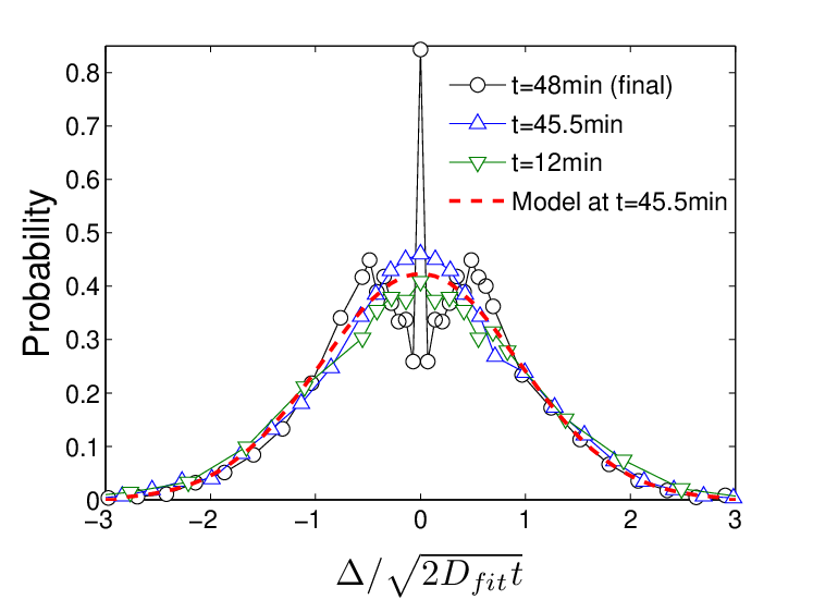
Finally, the scoring anomaly associated with the last 2.5 minutes of the game is striking. If the score evolves as an anti-persistent random walk, the distribution of the score difference should be Gaussian whose width grows with time as . As shown in Fig. 7, the distribution of score difference has a Gaussian appearance, with a width that grows slightly more slowly than . We attribute this small deviation to the weak restoring force, which gives a diffusion constant that decreases with time. However, in the final minutes of the game, the score-difference distribution develops a spike at and dips for small . Thus close games tend to end in ties much more often than expected from the random-walk picture of the score evolution. This anomaly may stems from the losing team playing urgently to force a tie, a hypothesis that accords with the observed increase in scoring rate near the end of the game (Fig. 1).
4 Computational Model
From all of the empirical observations about scoring, we now construct a computational random-walk model that broadly accounts for point-scoring statistical phenomena, as well as the win/loss record of all teams at the end of the season. In our model, games are viewed as a series of temporally homogeneous and uncorrelated scoring plays. The time between plays is drawn from a Poisson distribution whose mean is the observed value of seconds. We ignore the short-lived spikes and dips in the scoring rate at the end of each quarter (Fig. 1) and also the very rare plays of 5 or 6 points. Thus plays can be worth 1, 2, 3, or 4 points, with corresponding probabilities drawn from the observed distribution in Table 1. Simulations of scoring events continue until the final game time of minutes is reached.
There are three factors that determine which team scores. First, the better team has a greater intrinsic chance of scoring. The second factor is the anti-persistence of successive scoring events that arises from the change of possession after a score. The last is the linear restoring force, in which the scoring probability of a team decreases as its lead increases (and vice versa for a team in deficit). We therefore write the probabilities and that team A or team B scores next, immediately after a scoring event, as:
| (9) |
Here and are the intrinsic scoring probabilities (which must satisfy ; and the term accounts for the anti-persistence. Here is defined as
| (10) |
and ensures that the average probability for the same team to score twice in succession equals the observed value of 0.348. Finally, the term (with the score difference) accounts for the restoring force with the empirically measured restoring coefficient (Fig. 5).
In our minimalist model, the only distinguishing characteristic of team is its intrinsic strength . We estimate team strengths by fitting simulated team win/loss records to that predicted by the classic Bradley-Terry competition model (Bradley and Terry (1952)), in which the intrinsic scoring probabilities are given by
| (11) |
To simulate a season, we first assign a strength parameter to each team that is fixed for the season. We assume that the distribution of strengths is drawn from a Gaussian distribution with average and variance (James et al. (1993)). Nearly identical results arise for other team strength distributions. Since the intrinsic probabilities, and , depend only on the strength ratio , we may choose without loss of generality, so the only free parameter is . We determine by simulating many NBA seasons for a league of 30 teams for a range of values and comparing the simulated probability distributions for various fundamental game observables with corresponding empirical data.
Specifically, we examined: (i) The distribution of a given final score difference (already shown in Fig. 7). (ii) The season team winning percentage as a function of its normalized rank (Fig. 8 (a)); here, normalized rank is defined so that the team with the best winning percentage has rank 1, while the team with worst record has rank 0. (iii) The probability for a team to lead for a given fraction of the total game time (Fig. 8 (b)). (iv) The distribution of the number of lead changes during a game (Fig. 8 (c)).
Our motivation for focusing on these measures is that they provide useful statistical characterizations of how basketball games evolve. The score difference is the most basic information about the outcome of a basketball game. Similarly, the relation between rank and winning percentage provides a clean overall test of our model. The probability for a given lead time is motivated by the well-known, but mysterious arcsine law (Feller (1968)). According to this law, the trajectory of a one-dimensional random walk is likely to always be on one side of the origin rather than the walk spending equal amounts of time to the left and to the right of the origin. The ramification of the arcsine law for basketball is that a single team is likely to lead for the most of the game rather than both teams to equally sharing the time in the lead. As a corollary to the arcsine law, there are typically crossings of the origin for a one-dimensional random walk of steps, and the distribution in the number of lead changes is Gaussian. These origin crossings correspond to lead changes in basketball games.


For each of the four empirical observables listed above, we compare game data with the corresponding simulation results for a given value of the team strength variance . We quantify the quality of fit between the game data and the simulation results by the value defined by
| (12) |
Here is one of the four above-mentioned empirical observables, is the corresponding simulated observable, and is the underlying variable. For example, and could be the empirical and simulated probabilities of the final score difference and would be the final score difference.

Figure 9 shows the values of as a function of for the four observables. The best fit between the data and the simulations all occur when is in the range . To extract a single optimum value for , we combine the four measurements into a single function. Two simple and natural choices are the additive and multiplicative forms
| (13) |
where the sum and product are over the four observables, is associated with the observable, and is its minimum over all values. The denominator allows one to compare the quality of fit for disparate functions. In the absence of any prior knowledge about which statistical measure about basketball scoring is most important, we have chosen to weight them equally. With this choice, both and have minima at . Moreover, for this value of , the value of for each observable exceeds its minimum value by no more than . These results suggest that the best fit between our model and empirical data arises when we choose . Thus roughly 2/3 of the NBA teams have their intrinsic strength in the range .
5 Outlook
From all the play-by-play data of every NBA basketball game over four seasons, we uncovered several basic features of scoring statistics. First, the rate of scoring is nearly constant during a basketball game, with small correlations between successive scoring events. Consequently, the distribution of time intervals between scoring events has an exponential tail (Fig. 2). There is also a scoring anti-persistence, in which a score by one team, is likely to be followed by a score by the opponent because of the possession change after each basket. Finally, there is a small restoring force that tends to reduce the score difference between competitors, perhaps because a winning team coasts as its lead grows or a losing team plays more urgently as it falls behind.
Based on the empirical data, we argued that basketball scoring data is well described by a nearly unbiased continuous-time random walk, with the additional features of anti-persistence and a small restoring force. Even though there are differences in the intrinsic strengths of teams, these play a small role in the random-walk picture of scoring. Specifically, the dimensionless measure of the effect of disparities in team strength relative to stochasticity, the Péclet number, is small. The smallness of the Péclet number means that it is difficult to determine the superior team by observing a typical game, and essentially impossible by observing a short game segment. We simulated our random-walk model of scoring and found that it satisfyingly reproduces many statistical features about basketball scoring in NBA games.
This study raises several open issues. First, is the exponential distribution of time intervals between scoring events a ubiquitous feature of sports competitions? We speculate that perhaps other free-flowing games, such as lacrosse (Everson and Goldsmith-Pinkham (2008)), soccer (Dyte and Clarke (2000)), or hockey (Thomas (2007), Buttrey et al. (2011)), will have the same scoring pattern as basketball when the time intervals between scores are rescaled by the average scoring rate for each sport. It also seems plausible that other tactical metrics, such as the times intervals between successive crossings of mid-field by the game ball (or puck) may also be described by Poisson statistics. If borne out, perhaps there is a universal rule that governs the scoring time distribution in sports.
Seen through the lens of coaches, fans, and commentators, basketball is a complex sport that requires considerable analysis to understand and respond to its many nuances. A considerable industry has thus built up to quantify every aspect of basketball and thereby attempt to improve a team’s competitive standing. However, this competitive rat race largely eliminates systematic advantages between teams, so that all that remains, from a competitive standpoint, are small surges and ebbs in performance that arise from the underlying stochasticity of the game. Thus seen through the lens of the theoretical physicist, basketball is merely a random walk (albeit in continuous time and with some additional subtleties) and many of the observable consequences of the game follow from this random-walk description.
We thank Guoan Hu for assistance with downloading and processing the data and Ravi Heugel for initial collaborations on this project. We also thank Aaron Clauset for helpful comments on an earlier version of the manuscript. This work was supported in part by NSF grant DMR0906504.
References
- Albert et al. (2005) Albert, J., J. Bennett, and J. J. Cochran, eds. (2005): Anthology of Statistics in Sports, ASA-SIAM Series on Statistics and Applied Probability, volume 61, Philadelphia, PA: SIAM.
- Albert and Koning (2008) Albert, J. and R. H. Koning (2008): Statistical Thinking in Sports, Boca Raton: Taylor and Francis.
- Arkes and Martinez (2011) Arkes, J. and J. Martinez (2011): “Finally, Evidence for a Momentum Effect in the NBA,” J. Quantitative Analysis in Sports, 7.
- Ayton and Fischer (2004) Ayton, P. and I. Fischer (2004): “The hot hand fallacy and the gambler’s fallacy: Two faces of subjective randomness?” Memory & Cognition, 32, 1369.
- Box and Jenkins (1976) Box, G. E. P. and G. Jenkins (1976): Time Series Analysis: Forecasting and Control, Holden-Day.
- Bradley and Terry (1952) Bradley, R. A. and M. E. Terry (1952): “Rank Analysis of Incomplete Block Designs: I. The Method of Paired Comparisons,” Biometrika, 39, 324.
- Buttrey et al. (2011) Buttrey, S. E., A. R. Washburn, and W. L. Price (2011): “Estimating NHL Scoring Rates,” J. Quantitative Analysis in Sports, 7.
- de Saá Guerra et al. (2011) de Saá Guerra, Y., J. M. M. González, S. S. Montesdeoca, D. R. Ruiz, N. Arjonilla-López, and J. M. García-Manso (2011): “Basketball scoring in nba games: an example of complexity,” .
- Durham et al. (1998) Durham, Y., J. Hirschleifer, and V. L. Smith (1998): “Do the Rich Get Richer and the Poor Poorer? Experimental Tests of a Model of Power,” Am. Econ. Rev., 88, 891.
- Dyte and Clarke (2000) Dyte, D. and S. R. Clarke (2000): “A Ratings Based Poisson Model for World Cup Soccer Simulation,” J. Oper. Res. Soc., 51, 993.
- Everson and Goldsmith-Pinkham (2008) Everson, P. and P. S. Goldsmith-Pinkham (2008): “Composite Poisson Models for Goal Scoring,” J. Quantitative Analysis in Sports, 4.
- Feller (1968) Feller, W. (1968): An Introduction to Probability Theory and its Applications, volume 1, New York: Wiley.
- García-Pelayo (2007) García-Pelayo, R. (2007): “Solution of the persistent, biased random walk,” Physica A, 384, 143.
- Garfinkel and Skaperdas (2007) Garfinkel, M. and S. Skaperdas (2007): Handbook of Defense Economics, Amsterdam: Elsevier, North-Holland, volume 2, chapter 3, 649.
- Gilovich et al. (1985) Gilovich, T., R. Vallone, and A. Tversky (1985): “The Hot Hand in Basketball: On the Misperception of Random Sequences,” Appl. Cognitive Psych., 17, 295.
- Glickman and Evans (2009) Glickman, M. and S. Evans (2009): “The 2009 New England Symposium on Statistics in Sports,” J. Quantitative Analysis in Sports, 6.
- Gould (1996) Gould, S. J. (1996): Full House: The Spread of Excellence from Plato to Darwin, New York: Three Rivers Press.
- James et al. (1993) James, B., J. Albert, and H. S. Stern (1993): “Answering Questions About Baseball Using Statistics,” Chance, 6, 17–22.
- Kubatko et al. (2007) Kubatko, J., D. Oliver, K. Pelton, and D. T. Rosenbaum (2007): “A Starting Point for Analyzing Basketball Statistics,” J. Quantitative Analysis in Sports, 3.
- Miller and Weinberg (1991) Miller, S. and R. Weinberg (1991): “Perceptions of psychological momentum and their relationship to performance,” Sport Psychologist, 5, 211.
- Mosteller (1997) Mosteller, F. (1997): “Lessons from Sports Statistics,” Amer. Statistician, 51, 305–310.
- Probstein (1994) Probstein, R. F. (1994): Physicochemical Hydrodynamics, New York: J. S. Wiley & Sons, 2 edition.
- Redner (2001) Redner, S. (2001): A Guide to First-Passage Processes, New York: Cambridge University Press.
- Sire and Redner (2009) Sire, C. and S. Redner (2009): “Understanding baseball team standings and streaks,” Eur. Phys. Jour. B, 67, 473.
- Thomas (2007) Thomas, A. C. (2007): “Inter-arrival times of goals in ice hockey,” J. Quantitative Analysis in Sports, 3.
- Uhlenbeck and Ornstein (1930) Uhlenbeck, G. E. and L. S. Ornstein (1930): “On the theory of the Brownian motion,” Phys. Rev., 36, 823.
- Vergin (2000) Vergin, R. (2000): “Winning streaks in sports and the misperception of momentum,” J. Sports Behavior, 23, 181.
- Westfall (1990) Westfall, P. H. (1990): “Graphical Presentation of a Basketball Game,” Am. Statistician, 44, 305.