UOSTP 110801
Janus Black Holes
Dongsu Baka, Michael Gutperleb and Romuald A. Janikc
a Physics Department, University of Seoul, Seoul 130-743, Korea
b Department of Physics and Astronomy
University of California, Los Angeles, CA 90095, USA
c Institute of Physics, Jagiellonian University
Reymonta 4, 30-059 Kraków, Poland
dsbak@uos.ac.kr, gutperle@ucla.edu, romuald@th.if.uj.edu.pl
Abstract
In this paper Janus black holes in are considered. These are static solutions of an Einstein-scalar system with broken translation symmetry along the horizon. These solutions are dual to interface conformal field theories at finite temperature. An approximate solution is first constructed using perturbation theory around a planar BTZ black hole. Numerical and exact solutions valid for all sets of parameters are then found and compared. Using the exact solution the thermodynamics of the system is analyzed. The entropy associated with the Janus black hole is calculated and it is found that the entropy of the black Janus is the sum of the undeformed black hole entropy and the entanglement entropy associated with the defect.
1 Introduction
The Janus solutions [1] in various supergravity theories provide interesting realizations of interface conformal field theories within the AdS/CFT correspondence [2, 3, 4]. The simplest examples are constructed using an slicing of and making a massless field dependent on the slicing coordinate. Generically the scalar approaches two different constant values at the boundary of the space. Since a massless field is dual to a marginal operator the holographic interpretation is that the coupling constant associated with the marginal operator jumps across the interface. The nontrivial profile of the massless scalar breaks the full conformal symmetry but due to the factor the solution has interface conformal symmetry11 1 Many generalizations of Janus solutions have been found over the years, see e.g. [5, 6, 7, 8, 9, 10, 11, 12, 13]..
An important feature of the AdS/CFT correspondence is the fact that a black hole in the bulk of the AdS space is dual to a CFT at finite temperature [14]. It is natural to ask what is the bulk description of an interface CFT at finite temperature, i.e. a Janus black hole. In general this is a complicated problem due to the fact that a (planar) black hole in has translational invariance in the spatial directions. In a Janus solution the nontrivial scalar profile will break this translation invariance. Consequently a generic ansatz for a Janus black hole involves dependence on two spatial coordinates and hence solving nonlinear coupled partial differential equations, where numerical methods offer the only approach to solve the problem.
In this paper we will focus on the simplest case of the Janus black hole in three dimensions. The simplification is two fold, both the BTZ black hole solution as well as the Janus solution are simpler than in with . Secondly we find an exact analytical solution22 2 See also [13, 15, 16] for the other kinds of closely related exact solutions. for the Janus black hole which can be used to study analytically the physics of the interface CFT as well as test the numerical solution. Both simplifications are not present in higher dimensions but we believe that, as is often the case in AdS/CFT, there are valuable lessons to be learned from the lower dimensional exactly soluble system.
The structure of the paper is as follows: In section 2 we give a brief review of the Janus solution (at zero temperature) and the holographic calculation of the entanglement entropy of the interface CFT. In section 3 a small dilaton perturbation with a Janus profile around a planar BTZ black hole is constructed and it is shown that the boundary stress tensor is unchanged to leading order in the perturbation. The numerical solution for the Janus black hole is discussed in section 4. The main technical problem, that the domain of the coordinates is not fixed but dependent on the solution, is solved by using the dilaton itself as a coordinate. In section 5 the exact solution is constructed and used to test the accuracy of the numerical solution. In section 6 we calculate various thermodynamic quantities associated with the black Janus solution. In particular we calculate the entropy, being the horizon length of the black Janus solution, using two methods. First, we use a boundary-horizon map based on bulk conservation law considerations and second, we use a map which maps the boundary to the horizon using null geodesics. Interestingly both calculations give the same result and the entropy is the sum of the BTZ black hole entropy and the entanglement entropy of the zero temperature interface CFT. We close with a discussion of our results in section 7. Various details of calculations are relegated to appendices.
2 Janus system
In this section we will briefly review the construction of the three dimensional Janus solution [1, 13] and its holographic description as an interface conformal field theory (ICFT).
The three dimensional Janus solution can be embedded into ten dimensional type IIB supergravity by the following ansatz for the metric
| (2.1) |
where is either or . For the non supersymmetric Janus solution the dilaton and metric are independent of the coordinates of the three sphere and . All other type IIB supergravity fields are set to zero except the three-form field strength [13], whose explicit form is not needed in our later discussions. Upon dimensional reduction of the ten dimensional action on one arrives at three dimensional action for the metric and given by33 3 It is pointed out by Eoin Ó Colgáin that this three dimensional Janus system can also be consistently embedded into the eleven dimensional supergravity using the extra dimensional geometry [17]. This is dual to an interface version of the chiral SCFT in two dimensions.
| (2.2) |
From this action the Einstein equation becomes
| (2.3) |
and the scalar equation of motion is given by
| (2.4) |
For the static Janus solution the three dimensional metric and the dilaton take the following form
| (2.5) |
where we have set the radius to one for convenience. In [13] it was shown that the solution of the equations of motion (2.3) and (2.4) for this ansatz is given by
| (2.6) |
and
| (2.7) |
The Janus solution holographically realizes an ICFT where two CFTs defined on dimensional half spaces are glued together over a dimensional interface. This can be seen as follows: The conformal boundary of the metric (2.5) has three components as and finite we can strip off the factor and the boundary geometry are two copies of spanned by . Note that the dilaton approaches two constant values at the boundaries
| (2.8) |
Without loss of generality we may set . For later use it is also convenient to express in terms :
| (2.9) |
The values of the dilaton on the boundary is dual to a modulus of the two dimensional CFT. The third boundary component is at (i.e. the boundary of the factor) This defines the interface where the two half planes are glued together. Hence the dual CFT is an ICFT where two CFTs defined on a half line are at different points in their moduli space.
2.1 Entanglement entropy
A useful observable in the ICFT is the entanglement entropy which is defined as follows. The space on which the CFT is living is divided into two domains and . The total space of states is expressed product , where is supported on and respectively. A reduced density matrix can be defined by tracing over all states in ,
| (2.10) |
where is the density matrix of the total system (at zero temperature this is just the projector on the ground state). The entanglement entropy associated with the domain is then defined as
| (2.11) |
A holographic prescription to calculate the entanglement entropy in spaces which are asymptotic to was presented in [18, 19]. For the domain we denote the boundary which separates it from . A static minimal surface which extends into the bulk and ends on as one approaches the boundary of . The holographic entanglement entropy can then be calculated as
| (2.12) |
where denotes the area of the minimal surface and is the Newton constant for gravity.
In the present paper we consider the Janus deformation of and the area is an interval and the boundary are the two end points of the interval. The minimal surface is a space-like geodesic connecting the points. The geodesic which was used in [20] to compute the entanglement entropy chooses the coordinate as constant , while varies from to . This corresponds to a symmetric region of width around the interface.
The geodesic length is divergent and has to be regularized by introducing a cutoff near the boundary [20]
| (2.13) |
where the regularized length can be read off from (2.6)
| (2.14) |
Hence
| (2.15) | |||||
The holographic result has the same general form as the entanglement entropy calculated on the CFT side using the replica trick [21],
| (2.16) |
where we identify the length of the interval and is the UV cutoff. The last term is boundary entropy (sometimes called g-factor [22]) which is associated with the degrees of freedom localized on the interface. In Ref. [20] it was shown that in an expansion in the small deformation parameter the holographic result (2.15) agrees to leading order with the weakly-coupled CFT calculation of the boundary entropy. Note that in the supersymmetric generalization of the Janus solution [23, 24] one finds exact agreement to all orders. In Appendix A, we redo the leading order computation using conformal perturbation theory, which is valid for the strongly coupled limit.
3 Black Janus as a perturbation of the planar BTZ black hole
3.1 Planar BTZ Black Holes
We shall begin our discussion of three dimensional Janus black holes by studying the leading order corrections to the geometry and scalar field starting from the planar BTZ black hole solution. The planar BTZ black hole in three dimensions [25] can be written as
| (3.1) |
where we take the range of coordinate as . Of course the direction may be compactified on a circle but we shall be concerned here only with the non compact case. The horizon is located at and a convenient change of variables for checking its regularity is
| (3.2) |
In this coordinate system the black hole looks like
| (3.3) |
and now the AdS boundary is located at while the horizon at . Since
| (3.4) |
in the near horizon regime, there is no conical singularity if the euclidean time coordinate is periodic with period . Therefore the corresponding temperature can be identified as
| (3.5) |
The BTZ black hole with general temperature is described by the metric
| (3.6) |
which can be obtained by the scale coordinate transformation
| (3.7) |
from (3.1). The temperature for this scaled version of the black hole now becomes
| (3.8) |
Below we work mostly with the temperature and, using the above freedom of scale transformation, we shall recover the general temperature dependence whenever it is necessary.
3.2 Linearized Black Janus
Introducing a new coordinate given by , the planar black hole metric (3.1) can be rewritten as
| (3.9) |
Motivated by the form of this metric, we shall make the following ansatz for the black Janus solution
| (3.10) |
It is then straightforward to show that the equations of motion (2.3) and (2.4) reduce to
| (3.11) | |||
| (3.12) | |||
| (3.13) |
where we introduced the notation . To the leading order, the scalar equation can be integrated as
| (3.14) |
where we have used the Janus boundary condition with the sign function . The leading perturbation of the metric part is of order . For which we set
| (3.15) |
with
| (3.16) |
The leading order equations for the metric part becomes
| (3.17) | |||
| (3.18) |
With the Janus boundary condition whose detailed structure will be discussed later on, the solution can be found as where
| (3.19) |
with and being integration constants44 4 Only the combination is a true integration constant. We break it up to two since their roles are different in the discussions below.. Indeed checking that (3.19) solves eqs. (3.17-3.18) is straightforward. Then the metric for the black Janus can be written as
| (3.20) |
Next we introduce a new angular coordinate that is defined by
| (3.21) |
The above metric for the linearized black Janus can be written using the scale function of the original Janus solution: Namely, the metric can be expressed in the following form
| (3.22) |
where
| (3.23) |
with
| (3.24) | |||
| (3.25) | |||
| (3.26) |
To show this, we have used the expansion of the scale function given in the form
| (3.27) |
As will be explicitly verified later on, the remaining part of the metric except the scale factor possesses a translational isometric direction along . Hence one may set without loss of generality. The zeroes of the function and occur at , which correspond to the boundary of the asymptotically AdS space. As a consequence the coordinate is ranging over as the case of the original Janus solution.
The choice of the integration constant is simply related to the the choice of the coordinate patch of , which covers only part of the entire black hole geometry. Let us first consider the choice . Then the boundary occurs at
| (3.28) |
This is then solved by
| (3.29) |
Therefore the validity of the coordinate is limited by
| (3.30) |
and, hence, the coordinate along the boundary become singular if
| (3.31) |
Only the region can be free of any such coordinate problem. But this is simply a coordinate singularity, which may be removed by choosing a different coordinate chart. For instance let us consider the choice . For this case, one boundary can be solved by for , whose solution is . For this side we do not have any coordinate problem but the other side of the boundary has again the coordinate singularity. The region specified by of this coordinate chart does not involve any coordinate problem. By the choice of , the region can be safely covered, which includes the other side of the boundary.
For our further analysis of geometry below, we shall simply choose (together with ), since the presence of the coordinate singularity can be ignored in the small limit.
3.3 Boundary stress tensor
In this subsection, we shall construct the Fefferman-Graham metric to determine the boundary stress energy tensor. In order to use the prescription developed in Ref. [26], we introduce the metric in the following Fefferman-Graham form,
| (3.32) |
where () denote the boundary coordinates55 5 We use this notation of boundary coordinates for this subsection only. In the subsequent (sub)sections we shall simply use and for the boundary coordinates for the notational simplicity. and corresponds to the location of the boundary. In general one may expand by
| (3.33) |
where is the metric for the boundary system. In three dimensions, the boundary stress energy tensor is then given by [26]
| (3.34) |
where is the scalar contribution for the stress energy tensor given by
| (3.35) |
with denoting the boundary value of the scalar field. For our case, the boundary metric is given by
| (3.36) |
since the boundary system is defined in the flat Minkowski space in two dimensions and the scalar contribution to the stress energy tensor vanishes since the scalar field is constant except . Let us first bring the metric in (3.22) to the form
| (3.37) |
where . Introducing and by
| (3.38) |
and comparing the two forms of the metric to the leading order of , one finds the differential equations,
| (3.39) |
with
| (3.40) |
The boundary conditions are required to have the standard form of the boundary metric . The solution satisfying the boundary conditions is uniquely found by
| (3.41) | |||||
with
| (3.42) | |||||
One may check that the location of boundary in (3.29) corresponds to as expected.
For the stress energy tensor, we now note that , which implies that the terms have no contribution to the stress energy tensor. The rest is then straightforward: Noting
| (3.43) |
one finds
| (3.44) |
Therefore, one has
| (3.45) |
Hence to the leading order in , the stress energy tensor is independent of the deformation. Later on we shall show that is in fact independent and the zeroth order result is all order exact. Finally recovering the temperature dependence by the scaling transformation, we have
| (3.46) |
which agrees with that for the usual BTZ black hole.
4 Black Janus at arbitrary — Numerical Approach
In order to obtain the form of the Janus black hole in the fully nonlinear regime of arbitrary we develop a numerical approach to solving the relevant Einstein+dilaton system of equations. It turns out that a successful implementation is surprisingly subtle, due to the special features of the Janus system.
The most naive guess for the numerical ansatz would be
| (4.1) |
with the dilaton given by . This form of the metric ansatz makes it very easy to implement both constant temperature (which corresponds to Dirichlet boundary conditions for at and Neumann for ) and the Janus boundary condition. For numerics, we should map the infinite spatial coordinate into a finite interval e.g. by the mapping . However, this metric leads to several problems, some purely numerical and some, what is more dangerous, conceptual. Firstly, the discontinuous boundary condition for the dilaton with the jump at is very difficult to handle numerically. Secondly, it is far from clear what would be the domain of definition of the exact solution. The range of the bulk coordinate is , however the range of is unknown. At the boundary the range is , but in the bulk it may well be with an a-priori unknown profile . This indeterminacy a-priori precludes any numerical treatment.
In order to overcome the above difficulty, it is convenient to link the spatial coordinate to the value of the dilaton, since then the asymptotic range of the spatial coordinate is fixed by the definition of the Janus system, since at spatial infinities the dilaton is constant in the bulk and attains its asymptotic value . This leads to the following ansatz (recall (2.8))
| (4.2) | |||||
| (4.3) |
We have thus to deal with a non diagonal metric. Moreover it is not obvious what should be the boundary conditions characteristic of asymptotically AdS spacetime. To this end let us consider as a first approximation the BTZ black hole and use the linearized dilaton perturbation to fix the spatial coordinate according to (4.3).
The standard BTZ black hole metric is
| (4.4) |
where we introduced . Now the linearized Janus perturbation (3.14) takes the form
| (4.5) |
which leads to the following change of coordinates
| (4.6) |
In these ‘dilaton-adjusted’ coordinates the BTZ black hole takes the following form
| (4.7) |
which suggests the following ansatz for numerical computations
| (4.8) |
with very smooth solutions for : and . Performing numerics with such an ansatz shows that even for very small (equivalently ), the coefficient functions have different limits as with fixed and as keeping fixed. This leads to severe numerical problems and indicates that the pre-factor
| (4.9) |
should be replaced by a suitable -dependent function.
Fortunately, the Einstein-dilaton equations for the coefficient functions at reduce to ordinary differential equations with no -derivatives, which can be solved exactly. Particularly relevant is the solution for :
| (4.10) |
with
| (4.11) |
Taking into account the asymptotic BTZ metric at spatial infinity
| (4.12) |
we are led to modify the pre-factor
| (4.13) |
to take into account these properties, namely we require that
| (4.14) | |||||
| (4.15) |
In addition it is convenient to have and so as not to modify the form of boundary conditions at the horizon. A function which satisfies all the above properties is
| (4.16) |
This leads us to the final ansatz for the numerical solution:
| (4.17) |
At the horizon we impose the following boundary conditions:
| (4.18) |
The first condition ensures that the temperature is constant. At we impose boundary conditions following from symmetry
| (4.19) |
4.1 Numerical details
A feature of the Einstein’s equations for the coordinate ansatz (4.17) is that we can pick three independent first order equations. These are the equation for , the component of Einstein’s equations , and an appropriate linear combination of and . Subsequently we solve the above three equations numerically.
We use a Chebyshev grid of or points in each dimension and use the PETSc library for solving nonlinear equations. We use a Python interface to the library (petsc4py). Unfortunately the convergence is poor so we had to use an automatic differentiation package (ADOL-C with Python bindings pyadolc) to compute the Jacobian and use LU linear solver from PETSc instead of the standard iterative ones. In addition the numerical solutions were found by gradually increasing the asymptotic value of the dilaton by from the BTZ value of and using the output from the previous value of as initial conditions for . In this way we generated the metric profiles up to .
The above numerical setup should be readily generalizable to the Janus black holes in higher number of dimensions for which, almost certainly an analytical solution does not exist.
5 Black Janus at arbitrary — Exact solution in 3D
As an alternative to the direct numerical solutions, one may attempt to use the above properties of the metric, such as the form of (4.10) to try to obtain an exact analytical solution. Remarkably this can be done for the three dimensional black Janus system considered in this paper.

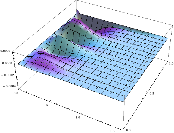
The exact Black Janus solution for arbitrary turns out to be given by the following analytical expression:
| (5.1) |
where
| (5.2) |
and
| (5.3) |
In this form we see the way that the exact metric incorporates the behavior (4.10). The similarity with the numerical ansatz made it easy to compare the above exact expression with the numerical solution for quite large value of with excellent agreement. In figure 1 we show the numerically obtained coefficient function from (4.17) together with the relative deviation from the exact solution obtained from (5.1).
It turns out, however, that passing to another coordinate system allows us to drastically simplify the metric. Indeed, let us change the coordinate into through the expression
| (5.4) |
Then the exact metric transforms into
| (5.5) |
This can be further simplified introducing the coordinate instead of through . With this substitution, we obtain a remarkably simple form of the exact Janus black hole metric:
| (5.6) | |||||
where we have used the fact with given by (3.23).
6 Thermodynamics and Entropy
6.1 Thermodynamic quantities
In this section, we shall be describing thermodynamic properties of our Janus system based on the solution of the previous section. First we turn to the stress energy tensor. We have already discussed the stress energy tensor for the case of the linearized black Janus and claimed that the expression in (3.46) is in fact exact to all orders in . Let us argue this point first. From the exact metric we note that the deformation parameter dependence occurs only through the function . In the near boundary region of , the scale function can be expanded as
| (6.1) |
and dependence can only appear in the higher order coefficients with . From dimensional analysis it follows that in the near boundary region where is the Fefferman-Graham coordinate introduced in (3.32). Hence and are independent since its dependence enters only at higher orders of . Therefore we conclude that the stress energy tensor in (3.46) is all order exact.
One can reach the same conclusions purely from the field theory perspective. Consider the energy-momentum conservation equations:
| (6.2) |
Due to time reversal invariance we have . Then is independent and, due to tracelessness, so is . So is diagonal and constant in space and time. For an infinite system that we consider explicitly here, the value of the energy density equals the value of the energy density in the asymptotic region and so equals the BTZ value.
Of course our expression of stress tensor is strictly valid only when the size of the boundary system goes to infinity. Dealing with the finite size system, which in general involves the finite size effect, is not a simple matter. According to the recent proposal [27], the boundary of a boundary system, can be dealt with in a rather simple manner by introducing corresponding bulk boundaries . This hypersurface is extended into the bulk in an appropriate manner from and introduces an extra contribution to the thermodynamic quantities. This formalism, however, is developed only for boundary conformal field theories and it is not clear whether it is applicable to our case or not. Thus in this note we shall be only concerning about the limit where the system size goes to infinity.
In the next two subsections, we shall be calculating the entropy of the black Janus system utilizing two different methods. Since the translational symmetry in the direction is broken by the Janus deformation, the entropy density should be position dependent. The entropy is a quantity defined at the horizon, whereas the interface CFT and its stress tensor is naturally defined at the boundary side of the geometry. Hence in order to talk about the entropy, one has to relate the horizon side to the boundary side. Especially one needs a map which relates the boundary coordinate to the horizon coordinate in order to use the data found at the horizon of the black hole. Below we shall discuss two methods for the boundary-horizon map, which will be used to determine the entropy of the boundary system. We shall find that the both methods lead to the desired entropy in the large limit to all orders in . Using the map, one may wonder whether one can define an entropy density by evaluating the corresponding horizon length scale divided by . The resulting expressions for the entropy density by the two methods turn out not to agree with each other even in the large limit. This, however, is not a problem. As discussed in [28], the entropy density alone is not fully well defined in a gauge invariant manner even in the semiclassical limit. We shall get back to this issue later in the discussion section.
6.2 Method 1
As stated previously, the entropy is a quantity which is defined at the horizon whereas the interface conformal field theory is defined at the boundary of the geometry. The stress energy tensor is also determined by the behavior of the geometry near the boundary. The question is how to connect a boundary region given by to the corresponding horizon region as depicted in Figure 2. In other words the question is how to find the two bulk lines and which join the image at the horizon to the boundary region (of a coordinate size ). This may be done as follows: Consider the conserved current [29]
| (6.3) |
where is the time translation Killing vector satisfying the Killing equation . In our case, and one may find the boundary lines from the condition
| (6.4) |
with . This basically says that there is no contribution from the bulk lines for the integral of over the region surrounded by . This condition then ensures the first law of thermodynamics that connects the change of entropy to the energy and the length of the system.

For the analysis of the exact geometry, we shall use the metric in (5.6). As in the previous section, we shall consider the boundary system of spatial size with the interface at the center. (Namely with as the standard boundary coordinate.) Following above prescription, the corresponding bulk lines satisfy
| (6.5) |
This is solved by
| (6.6) |
For the line starting from ,
| (6.7) |
This identification of the boundary coordinate for exact black Janus solution is carried out in Appendix C. The corresponding horizon point is described by
| (6.8) |
together with . This is exactly the boundary-horizon map obtained by the present method. Then the horizon length can be obtained by
| (6.9) |
where we used
| (6.10) |
The entropy then becomes
| (6.11) |
By expanding in , one may find the leading order behavior as
| (6.12) |
For the large size limit the finite part of (6.11) becomes
| (6.13) |
This expression precisely coincides with the result from the method of the holographic entanglement entropy.
6.3 Method 2: a boundary horizon map based on null geodesics
In this subsection, we shall carry out the boundary horizon map based on the null geodesics emanating from the boundary in a hypersurface orthogonal manner. This construction is based on the concept of the light-sheet of the holography [30] and widely used in application of fluid-geometry correspondence [28, 31, 32, 33].
Since null geodesics are the same for conformally equivalent metrics it is enough to determine them for the metric
| (6.14) |
where we have
| (6.15) | |||||
| (6.16) |
The geodesic equations read
| (6.17) | |||||
| (6.18) | |||||
| (6.19) |
and the null condition is
| (6.20) |
It is convenient to parameterize the geodesics with instead of the affine parameter . One can check that the solution is
| (6.21) | |||||
| (6.22) | |||||
| (6.23) |
As mentioned above, at the horizon is , while approaching the boundary point leads to
| (6.24) |
in agreement with (6.7). In order to determine which geodesic to take we have to fix the direction of the null geodesic emitted from the boundary. In the following we utilize the coordinates which are defined in appendix C. Near the boundary this requirement means that we follow a curve of fixed . We have to translate this condition to a condition on the derivative
| (6.25) |
at . To this end we have
| (6.26) |
where the derivatives have to be taken along constant . We can evaluate the last derivative by differentiating
| (6.27) |
with respect to and taking the limit . From this we see that is finite which means that
| (6.28) |
Evaluating gives
| (6.29) |
Hence this condition enables us to identify the constant
| (6.30) |
Now the geodesic takes the following form in the - plane:
| (6.31) |
where corresponds to . Evaluating the above expression at the horizon we get
| (6.32) |
This is the boundary-horizon map based on null geodesics. By inspection we see that it is different from the one in (6.8).
If we take (), and we recover which is the expected result. However one may be puzzled by the opposite limit. When which should correspond to , does not approach 0 but rather
| (6.33) |
As an aside, from the general formula for we see that at the horizon the geodesic is always perpendicular to the horizon so the latter condition does not allow us to discriminate between geodesics.
Based on the above boundary-horizon map in (6.32), the horizon length is given by
| (6.34) |
We also rewrite (6.32) as
| (6.35) |
From this formula, we would like to identify the leading order correction of the entropy. Noting
| (6.36) |
one finds
| (6.37) |
In addition, the Jacobi sine function can be expanded as
| (6.38) |
From this, one finds
| (6.39) |
Interestingly, this leads to
| (6.40) |
as becomes infinity. Thus we obtained the expected result to this order. Let us now rewrite (6.34) as
| (6.41) |
Then using
| (6.42) |
one finds
| (6.43) |
Again this leads to
| (6.44) |
which agrees with the result of the holographic entanglement.
6.4 Remarks on the agreement between the two methods
Let us discuss now what aspects of the boundary-horizon map are probed by the above calculations of the agreement between the entanglement entropy and the two computations using the two choices of the boundary-horizon map.
If the size of the system would be finite (with a circle compactification), then the total entropy would be obviously completely independent of the choice of the boundary-horizon map as it has a purely geometrical definition as the area (length in the 3D case) of the horizon. In the case of the infinite system that we consider, we have to subtract off the extensive contribution – and hence a potential difference may arise only in the upper limit of integration of the horizon area element. Therefore we are probing differences between the boundary-horizon maps in the asymptotic near BTZ region. Unfortunately, so far we do not have a test which would be sensitive to the finer details of the boundary-horizon map closer to the defect.
6.5 First law of thermodynamics
From the previous investigation, the entropy of the system in the large size limit is given by
| (6.45) |
where denotes in (6.44) and we have recovered the temperature dependence. is temperature independent and can be interpreted as the localized interface contribution to the entropy. From the stress tensor in (3.46), the energy and pressure can be identified as
| (6.46) |
Therefore one can check that the first law of thermodynamics
| (6.47) |
holds precisely for our Janus system. Of course one should note that our investigation is valid only for the large size limit.
7 Conclusion
In the present paper we have considered a supergravity dual to a three-dimensional interface conformal field theory at finite temperature. The supergravity fields which are turned on are the metric and the dilaton. The interface is realized as the boundary between two domains ( and ) with differing values of the vacuum expectation value of the operator dual to the dilaton .
The undeformed finite temperature case corresponds to the well-known BTZ black hole. We have started from a linearized analysis of the scalar perturbation with small of the BTZ black hole building up intuitions concerning the general structure of the solution including the extraction of the boundary energy-momentum tensor which is quite intricate in coordinates natural for the Janus solution.
Using this knowledge we have formulated a scheme suitable for the numerical computation of the exact Janus black hole for arbitrary , the key obstacle being an a-priori lack of knowledge about the coordinate domain of the exact nonlinear solution. We overcame this problem by linking a spatial coordinate to the value of the dilaton.
In the case of three-dimensional system we found an exact analytical solution of the finite-temperature Janus black hole. Let us emphasize that, due to the coupling between gravity and the scalar field, the three-dimensional Einstein-dilaton system is nontrivial in contrast to pure three-dimensional gravity. The existence of an analytical exact solution was in fact completely unexpected for us.
This exact solution is very interesting from various points of view. On the general relativity side it provides an example of a black hole in equilibrium with a nonuniform horizon. It would be very interesting to explore such features as Hawking radiation and temperature in this setting.
From the AdS/CFT perspective, such a black-hole gives a dual description of a three-dimensional interface CFT at finite temperature, which may have condensed matter applications. On a more theoretical side, such a nonuniform black hole provides a theoretical laboratory for investigating various issues dealing with entropy of the dual field theory. In particular, we can probe various maps between boundary points and horizon points which have been proposed in the literature, and critically examine the problem whether local entropy density can be defined at all.
As a step in this direction we have evaluated the total entropy deviation from the BTZ answer using two different boundary-bulk map prescriptions finding agreement with entanglement entropy calculations.
There are numerous directions for further research. First, one may also consider ICFT defined on a circle with two interface points. Of course there is a corresponding Janus solution dual to this compact version of ICFT. This system can serve as an ideal setup to study finite size effects of a finite temperature ICFT. Secondly one can investigate the gravitational aspects of the nonuniform horizon, generalize the setup to higher number of dimensions (where probably one would have to rely on numerical methods). One new nontrivial feature in higher dimensions may be the appearance of nonuniform energy density which is kinematically ruled out in the three-dimensional case. It would also be an interesting question to explore if and how the presence of an interface modifies the occurrence of a phase transition (such as a confinement/deconfinement transition) in AdS/CFT.
Acknowledgement
We would like to thank Shiraz Minwalla, Tadashi Takayanagi and Hyunsoo Min for helpful discussions. DB was supported in part by NRF SRC-CQUeST-2005-0049409 and NRF Mid-career Researcher Program 2011-0013228. MG was supported in part by NSF grant PHY-07-57702. RJ was supported by Polish science funds as a research project N N202 105136 (2009-2012).
Appendix A Computation of entropy correction based on the conformal perturbation theory
In this appendix we are interested in computing free energy defined by
| (A.1) |
Perturbing the above from of BTZ system, one has
| (A.2) |
The contribution vanishes because
| (A.3) |
where the expectation value is evaluated with respect to the BTZ system with . And one can find
| (A.4) |
where is the sign function. Note that the two point function [15] is given by
| (A.5) |
for the BTZ background with . Using the integral
| (A.6) |
can be rearranged as
| (A.7) |
with . Using the symmetry of the integrand, the integral may be further arranged as
| (A.8) |
where we also introduce a finite system size . This regularized integral is finite and has the expansion,
| (A.9) |
where dependence in the leading term is introduced by the dimensional ground. is not physical since it reflects our choice of the vacuum energy level. We evaluate the integral (A.8) by the replacement of the integrand by
| (A.10) |
which does not affect , and terms in the expansion. This fact may be checked numerically, whose details are in Appendix B. Thus, by the replacement, the physical term is not affected.
Then the integral may be carried out explicitly leading to
| (A.11) |
which can be expanded as
| (A.12) |
Therefore one has
| (A.13) |
as the size becomes large.
Note that our computation here does not care about possible finite size effect. Namely any effect of boundary conditions at was not incorporated into the computation above. Including the finite size effects on the field theory side is an interesting open problem.
Appendix B Equivalence of and to
We are interested in the integral
| (B.1) |
where
| (B.2) |
We will show that
| (B.3) |
Using an integration by parts and a change of variables, one may rearrange as
| (B.4) |
We then expand the integrand into a power series in and perform the integral order by order. And then expand the result again into a power series in , which leads to the series expansion of (B.3) in . For instance by expanding the integrand to the order , we get
| (B.5) |
which agrees with the expansion of (B.3). This check can be pushed further to the higher orders in .
Appendix C The boundary metric and coordinates of exact solution
In this appendix we shall construct the boundary metric from the exact solution (5.1). For this we have to pass to the Fefferman-Graham coordinates but just at the leading order. In order to approach the boundary we will take the limit in a correlated manner with namely
| (C.1) |
keeping fixed. From the exact metric, one finds
| (C.2) |
The exact Janus BH metric reads then in the coordinates at leading order in :
| (C.3) |
where
| (C.4) |
The boundary coordinate is then found from
| (C.5) |
Straightforward integration leads to
| (C.6) |
which can be inverted to yield
| (C.7) |
Finally using (C.2), one finds
| (C.8) |
References
- [1] D. Bak, M. Gutperle and S. Hirano, “A dilatonic deformation of AdS(5) and its field theory dual,” JHEP 0305, 072 (2003) [arXiv:hep-th/0304129].
- [2] J. M. Maldacena, “The large N limit of superconformal field theories and supergravity,” Adv. Theor. Math. Phys. 2, 231 (1998) [Int. J. Theor. Phys. 38, 1113 (1999)] [arXiv:hep-th/9711200].
- [3] S. S. Gubser, I. R. Klebanov and A. M. Polyakov, “Gauge theory correlators from non-critical string theory,” Phys. Lett. B 428 (1998) 105 [arXiv:hep-th/9802109].
- [4] E. Witten, “Anti-de Sitter space and holography,” Adv. Theor. Math. Phys. 2 (1998) 253 [arXiv:hep-th/9802150].
- [5] E. D’Hoker, J. Estes and M. Gutperle, “Exact half-BPS Type IIB interface solutions. I. Local solution and supersymmetric Janus,” JHEP 0706 (2007) 021 [arXiv:0705.0022 [hep-th]].
- [6] E. D’Hoker, J. Estes, M. Gutperle and D. Krym, “Exact Half-BPS Flux Solutions in M-theory. I: Local Solutions,” JHEP 0808 (2008) 028 [arXiv:0806.0605 [hep-th]].
- [7] M. Chiodaroli, M. Gutperle and D. Krym, “Half-BPS Solutions locally asymptotic to AdS(3) x S**3 and interface conformal field theories,” JHEP 1002 (2010) 066 [arXiv:0910.0466 [hep-th]].
- [8] E. D’Hoker, J. Estes and M. Gutperle, “Gravity duals of half-BPS Wilson loops,” JHEP 0706 (2007) 063 [arXiv:0705.1004 [hep-th]].
- [9] A. Clark and A. Karch, “Super Janus,” JHEP 0510, 094 (2005) [arXiv:hep-th/0506265].
- [10] O. Lunin, “1/2-BPS states in M theory and defects in the dual CFTs,” JHEP 0710, 014 (2007) [arXiv:0704.3442 [hep-th]].
- [11] J. Kumar and A. Rajaraman, “Supergravity solutions for branes,” Phys. Rev. D 69 (2004) 105023 [arXiv:hep-th/0310056].
- [12] M. Chiodaroli, E. D’Hoker, Y. Guo and M. Gutperle, “Exact half-BPS string-junction solutions in six-dimensional supergravity,” arXiv:1107.1722 [hep-th].
- [13] D. Bak, M. Gutperle and S. Hirano, “Three dimensional Janus and time-dependent black holes,” JHEP 0702 (2007) 068 [arXiv:hep-th/0701108].
- [14] E. Witten, “Anti-de Sitter space, thermal phase transition, and confinement in gauge theories,” Adv. Theor. Math. Phys. 2, 505 (1998) [arXiv:hep-th/9803131].
- [15] D. Bak, M. Gutperle and A. Karch, “Time dependent black holes and thermal equilibration,” JHEP 0712, 034 (2007) [arXiv:0708.3691 [hep-th]].
- [16] D. Bak, “Dual of big-bang and big-crunch,” Phys. Rev. D 75, 026003 (2007) [arXiv:hep-th/0603080].
- [17] E. O Colgain and H. Samtleben, JHEP 1102, 031 (2011) [arXiv:1012.2145 [hep-th]].
- [18] S. Ryu and T. Takayanagi, “Holographic derivation of entanglement entropy from AdS/CFT,” Phys. Rev. Lett. 96 (2006) 181602 [arXiv:hep-th/0603001].
- [19] S. Ryu and T. Takayanagi, “Aspects of holographic entanglement entropy,” JHEP 0608 (2006) 045 [arXiv:hep-th/0605073].
- [20] T. Azeyanagi, A. Karch, T. Takayanagi and E. G. Thompson, “Holographic Calculation of Boundary Entropy,” JHEP 0803 (2008) 054 [arXiv:0712.1850 [hep-th]].
- [21] P. Calabrese and J. L. Cardy, “Entanglement entropy and quantum field theory,” J. Stat. Mech. 0406 (2004) P002 [arXiv:hep-th/0405152].
- [22] I. Affleck and A. W. W. Ludwig, “Universal noninteger ’ground state degeneracy’ in critical quantum systems,” Phys. Rev. Lett. 67 (1991) 161.
- [23] M. Chiodaroli, M. Gutperle and L. Y. Hung, “Boundary entropy of supersymmetric Janus solutions,” JHEP 1009, 082 (2010) [arXiv:1005.4433 [hep-th]].
- [24] M. Chiodaroli, M. Gutperle, L. -Y. Hung, D. Krym, “String Junctions and Holographic Interfaces,” Phys. Rev. D83, 026003 (2011). [arXiv:1010.2758 [hep-th]].
- [25] M. Banados, C. Teitelboim and J. Zanelli, “The Black hole in three-dimensional space-time,” Phys. Rev. Lett. 69, 1849 (1992) [arXiv:hep-th/9204099].
- [26] S. de Haro, S. N. Solodukhin and K. Skenderis, “Holographic reconstruction of space-time and renormalization in the AdS / CFT correspondence,” Commun. Math. Phys. 217, 595 (2001) [arXiv:hep-th/0002230].
- [27] T. Takayanagi, “Holographic Dual of BCFT,” arXiv:1105.5165 [hep-th].
- [28] S. Bhattacharyya, V. E. Hubeny, R. Loganayagam, G. Mandal, S. Minwalla, T. Morita, M. Rangamani, H. S. Reall, “Local Fluid Dynamical Entropy from Gravity,” JHEP 0806 (2008) 055. [arXiv:0803.2526 [hep-th]].
- [29] V. Iyer and R. M. Wald, “Some properties of Noether charge and a proposal for dynamical black hole entropy,” Phys. Rev. D 50, 846 (1994) [arXiv:gr-qc/9403028].
- [30] R. Bousso, “A Covariant entropy conjecture,” JHEP 9907 (1999) 004 [arXiv:hep-th/9905177].
- [31] P. M. Chesler, L. G. Yaffe, “Horizon formation and far-from-equilibrium isotropization in supersymmetric Yang-Mills plasma,” Phys. Rev. Lett. 102 (2009) 211601. [arXiv:0812.2053 [hep-th]].
- [32] I. Booth, M. P. Heller, M. Spalinski, “Black Brane Entropy and Hydrodynamics,” Phys. Rev. D83 (2011) 061901. [arXiv:1010.6301 [hep-th]].
- [33] M. P. Heller, R. A. Janik, P. Witaszczyk, “The characteristics of thermalization of boost-invariant plasma from holography,” [arXiv:1103.3452 [hep-th]].