跳到论文正文
W Papers独立论文阅读器 arXiv:1109.2694 论文正文 计算阅读时间 · 0%
引用这篇论文根据当前论文元数据生成,正式投稿前建议核对。


License: arXiv.org perpetual non-exclusive license
arXiv:1109.2694v5 [math.ST] 01 May 2014

Kernel density estimation for stationary random fields

Mohamed EL MACHKOURI

Laboratoire de Mathématiques Raphaël Salem
UMR CNRS 6085, Université de Rouen (France)
mohamed.elmachkouri@univ-rouen.fr

Abstract

In this paper, under natural and easily verifiable conditions, we prove the 𝕃1\mathbb{L}^{1}-convergence and the asymptotic normality of the Parzen-Rosenblatt density estimator for stationary random fields of the form Xk=g⁡(εk−s,s∈ℤd)X_{k}=g\left(\varepsilon_{k-s},s\in\mathbb{Z}^{d}\right), k∈ℤdk\in\mathbb{Z}^{d}, where (εi)i∈ℤd(\varepsilon_{i})_{i\in\mathbb{Z}^{d}} are independent and identically distributed real random variables and gg is a measurable function defined on ℝℤd\mathbb{R}^{\mathbb{Z}^{d}}. Such kind of processes provides a general framework for stationary ergodic random fields. A Berry-Esseen’s type central limit theorem is also given for the considered estimator.

AMS Subject Classifications (2000): 60F05, 60G60, 62G07, 62G20.
Key words and phrases: Central limit theorem, spatial processes, m-dependent random fields, physical dependence measure, nonparametric estimation, kernel density estimator, rate of convergence.
Short title: Kernel density estimation for random fields.

1 Introduction and main results

Let (Xi)i∈ℤ(X_{i})_{i\in\mathbb{Z}} be a stationary sequence of real random variables defined on a probability space (Ω,ℱ,ℙ)(\Omega,\mathcal{F},\mathbb{P}) with an unknown marginal density ff. The kernel density estimator fnf_{n} of ff introduced by Rosenblatt [19] and Parzen [18] is defined for all positive integer nn and any real xx by

fn​(x)=1n​bn​∑i=1nK​(x−Xibn)f_{n}(x)=\frac{1}{nb_{n}}\sum_{i=1}^{n}\text{K}\left(\frac{x-X_{i}}{b_{n}}\right)

where K is a probability kernel and the bandwidth bnb_{n} is a parameter which converges slowly to zero such that n​bnnb_{n} goes to infinity. The literature dealing with the asymptotic properties of fnf_{n} when the observations (Xi)i∈ℤ(X_{i})_{i\in\mathbb{Z}} are independent is very extensive (see Silverman [21]). Parzen [18] proved that when (Xi)i∈ℤ(X_{i})_{i\in\mathbb{Z}} are independent and identically distribut (i.i.d) and the bandwidth bnb_{n} goes to zero such that n​bnnb_{n} goes to infinity then (n​bn)1/2​(fn​(x0)−𝔼​fn​(x0))(nb_{n})^{1/2}(f_{n}(x_{0})-\mathbb{E}f_{n}(x_{0})) converges in distribution to the normal law with zero mean and variance f⁡(x0)​∫ℝK2​(t)​𝑑tf(x_{0})\int_{\mathbb{R}}\text{K}^{2}(t)dt. Under the same conditions on the bandwidth, this result was extended by Wu an Mielniczuk [26] for causal linear processes with i.i.d. innovations and by Dedecker and Merlevède [9] for strongly mixing sequences.
In this paper, we are interested by the kernel density estimation problem in the setting of dependent random fields indexed by ℤd\mathbb{Z}^{d} where dd is a positive integer. The question is not trivial since ℤd\mathbb{Z}^{d} does not have a natural ordering for d≥2d\geq 2. In recent years, there is a growing interest in asymptotic properties of kernel density estimators for random fields. One can refer for example to Carbon et al. ([2], [3]), Cheng et al. [7], El Machkouri [11], Hallin et al. [14], Tran [22] and Wang and Woodroofe [23]. In [22], the asymptotic normality of the kernel density estimator for strongly mixing random fields was obtained using the Bernstein’s blocking technique and coupling arguments. Using the same method, the case of linear random fields with i.i.d. innovations was handled in [14]. In [11], the central limit theorem for the Parzen-Rosenblatt estimator given in [22] was improved using the Lindeberg’s method (see [17]) which seems to be better than the Bernstein’s blocking technique approach. In particular, a simple criterion on the strong mixing coefficients is provided and the only condition imposed on the bandwith is nd​bn→∞n^{d}b_{n}\to\infty which is similar to the usual condition imposed in the independent case (see Parzen [18]). In [11], the regions where the random field is observed are reduced to squares but a carrefull reading of the proof allows us to state that the main result in [11] still holds for very general regions Λn\Lambda_{n}, namely those which the cardinality |Λn||\Lambda_{n}| goes to infinity such that |Λn|​bn|\Lambda_{n}|b_{n} goes to zero as nn goes to infinity (see Assumption (A3) below). In [7], Cheng et al. investigated the asymptotic normality of the kernel density estimator for linear random fields with i.i.d. innovations using a martingale approximation method (initiated by Cheng and Ho [6]) but it seems that there is a mistake in their proof (see Remark 6 in [23]). Since the mixing property is often unverifiable and might be too restrictive, it is important to provide limit theorems for nonmixing and possibly nonlinear random fields. We consider in this work a field (Xi)i∈ℤd(X_{i})_{i\in\mathbb{Z}^{d}} of identically distributed real random variables with an unknown marginal density ff such that

Xi=g⁡(εi−s,s∈ℤd),i∈ℤd,X_{i}=g\left(\varepsilon_{i-s};\,s\in\mathbb{Z}^{d}\right),\quad i\in\mathbb{Z}^{d}, (1)

where (εj)j∈ℤd(\varepsilon_{j})_{j\in\mathbb{Z}^{d}} are i.i.d. random variables and gg is a measurable function defined on ℝℤd\mathbb{R}^{\mathbb{Z}^{d}}. In the one-dimensional case (d=1d=1), the class (1) includes linear as well as many widely used nonlinear time series models as special cases. More importantly, it provides a very general framework for asymptotic theory for statistics of stationary time series (see e.g. [24] and the review paper [25]).
We introduce the physical dependence measure first introduced by Wu [24]. Let (εj′)j∈ℤd(\varepsilon_{j}^{{}^{\prime}})_{j\in\mathbb{Z}^{d}} be an i.i.d. copy of (εj)j∈ℤd(\varepsilon_{j})_{j\in\mathbb{Z}^{d}} and consider for all positive integer nn the coupled version Xi∗X_{i}^{\ast} of XiX_{i} defined by Xi∗=g⁡(εi−s∗,s∈ℤd)X_{i}^{\ast}=g\left(\varepsilon^{\ast}_{i-s}\,;\,s\in\mathbb{Z}^{d}\right) where εj∗=εj11{j≠0}+ε0′11{j=0}\varepsilon_{j}^{\ast}=\varepsilon_{j}\,\hbox to0.0pt{\mbox{\small\rm 1}\hss}\kern 1.49994pt1_{\{j\neq 0\}}+\varepsilon_{0}^{{}^{\prime}}\,\hbox to0.0pt{\mbox{\small\rm 1}\hss}\kern 1.49994pt1_{\{j=0\}} for all jj in ℤd\mathbb{Z}^{d}. In other words, we obtain Xi∗X_{i}^{\ast} from XiX_{i} by just replacing ε0\varepsilon_{0} by its copy ε0′\varepsilon_{0}^{{}^{\prime}}. Let ii in ℤd\mathbb{Z}^{d} and p>0p>0 be fixed. If XiX_{i} belongs to 𝕃p\mathbb{L}_{p} (that is, 𝔼​|Xi|p\mathbb{E}|X_{i}|^{p} is finite), we define the physical dependence measure δi,p=‖Xi−Xi∗‖p\delta_{i,p}=\|X_{i}-X_{i}^{\ast}\|_{p} where ∥.∥p\|\,.\,\|_{p} is the usual 𝕃p\mathbb{L}^{p}-norm and we say that the random field (Xi)i∈ℤd(X_{i})_{i\in\mathbb{Z}^{d}} is pp-stable if ∑i∈ℤdδi,p<∞\sum_{i\in\mathbb{Z}^{d}}\delta_{i,p}<\infty. For d≥2d\geq 2, the reader should keep in mind the following two examples already given in [12] :
Linear random fields: Let (εi)i∈ℤd(\varepsilon_{i})_{i\in\mathbb{Z}^{d}} be i.i.d random variables with εi\varepsilon_{i} in 𝕃p\mathbb{L}^{p}, p≥2p\geq 2. The linear random field XX defined for all ii in ℤd\mathbb{Z}^{d} by

Xi=∑s∈ℤdas​εi−sX_{i}=\sum_{s\in\mathbb{Z}^{d}}a_{s}\varepsilon_{i-s}

with (as)s∈ℤd(a_{s})_{s\in\mathbb{Z}^{d}} in ℝℤd\mathbb{R}^{\mathbb{Z}^{d}} such that ∑i∈ℤdai2<∞\sum_{i\in\mathbb{Z}^{d}}a_{i}^{2}<\infty is of the form (1)(\ref{definition_champ}) with a linear functional gg. For all ii in ℤd\mathbb{Z}^{d}, δi,p=|ai|∥ε0−ε′0∥p\delta_{i,p}=|a_{i}|\|\varepsilon_{0}-\varepsilon^{{}^{\prime}}_{0}\|_{p}. So, XX is pp-stable if ∑i∈ℤd|ai|<∞\sum_{i\in\mathbb{Z}^{d}}|a_{i}|<\infty. Clearly, if H is a Lipschitz continuous function, under the above condition, the subordinated process Yi=H​(Xi)Y_{i}=\textrm{H}(X_{i}) is also pp-stable since δi,p=O⁡(|ai|)\delta_{i,p}=O(|a_{i}|).
Volterra field : Another class of nonlinear random field is the Volterra process which plays an important role in the nonlinear system theory (Casti [4], Rugh [20]): consider the second order Volterra process

Xi=∑s1,s2∈ℤdas1,s2​εi−s1​εi−s2,\displaystyle X_{i}=\sum_{s_{1},s_{2}\in\mathbb{Z}^{d}}a_{s_{1},s_{2}}\varepsilon_{i-s_{1}}\varepsilon_{i-s_{2}},

where as1,s2a_{s_{1},s_{2}} are real coefficients with as1,s2=0a_{s_{1},s_{2}}=0 if s1=s2s_{1}=s_{2} and (εi)i∈ℤd(\varepsilon_{i})_{i\in\mathbb{Z}^{d}} are i.i.d. random variables with εi\varepsilon_{i} in 𝕃p\mathbb{L}^{p}, p≥2p\geq 2. Let

Ai=∑s1,s2∈ℤd(as1,i2+ai,s22)andBi=∑s1,s2∈ℤd(|as1,i|p+|ai,s2|p).\displaystyle A_{i}=\sum_{s_{1},s_{2}\in\mathbb{Z}^{d}}(a_{s_{1},i}^{2}+a_{i,s_{2}}^{2})\quad\textrm{and}\quad B_{i}=\sum_{s_{1},s_{2}\in\mathbb{Z}^{d}}(|a_{s_{1},i}|^{p}+|a_{i,s_{2}}|^{p}).

By the Rosenthal inequality, there exists a constant Cp>0C_{p}>0 such that

δi,p=‖Xi−Xi∗‖p≤Cp​Ai1/2​‖ε0‖2​‖ε0‖p+Cp​Bi1/p​‖ε0‖p2.\displaystyle\delta_{i,p}=\|X_{i}-X_{i}^{*}\|_{p}\leq C_{p}A_{i}^{1/2}\|\varepsilon_{0}\|_{2}\|\varepsilon_{0}\|_{p}+C_{p}B_{i}^{1/p}\|\varepsilon_{0}\|_{p}^{2}.

From now on, for all finite subset Λ\Lambda of ℤd\mathbb{Z}^{d}, we denote |Λ||\Lambda| the number of elements in Λ\Lambda and we observe (Xi)i∈ℤd(X_{i})_{i\in\mathbb{Z}^{d}} on a sequence (Λn)n≥1(\Lambda_{n})_{n\geq 1} of finite subsets of ℤd\mathbb{Z}^{d} which only satisfies |Λn||\Lambda_{n}| goes to infinity as nn goes to infinity. It is important to note that we do not impose any condition on the boundary of the regions Λn\Lambda_{n}. The density estimator fnf_{n} of ff is defined for all positive integer nn and any real xx by

fn​(x)=1|Λn|​bn​∑i∈ΛnK​(x−Xibn)f_{n}(x)=\frac{1}{|\Lambda_{n}|b_{n}}\sum_{i\in\Lambda_{n}}\text{K}\left(\frac{x-X_{i}}{b_{n}}\right)

where bnb_{n} is the bandwidth parameter and K is a probability kernel. Our aim is to provide sufficient conditions for the 𝕃1\mathbb{L}_{1}-distance between fnf_{n} and ff to converge to zero (Theorem 1) and for (|Λn|​bn)1/2​(fn​(xi)−𝔼​fn​(xi))1≤i≤k,(xi)1≤i≤k∈ℝk,k∈ℕ\{0},(|\Lambda_{n}|b_{n})^{1/2}(f_{n}(x_{i})-\mathbb{E}f_{n}(x_{i}))_{1\leq i\leq k},\,(x_{i})_{1\leq i\leq k}\in\mathbb{R}^{k},\,k\in\mathbb{N}\backslash\{0\}, to converge in law to a multivariate normal distribution (Theorem 2) under minimal conditions on the bandwidth parameter. We give also a Berry-Esseen’s type central limit theorem for the considered estimator (Theorem 3). In the sequel, we denote |i|=max1≤k≤d⁡|ik||i|=\max_{1\leq k\leq d}|i_{k}| for all i=(i1,…,id)∈ℤdi=(i_{1},...,i_{d})\in\mathbb{Z}^{d} and we denote also δi\delta_{i} for δi,2\delta_{i,2}. The following assumptions are required.

  • (A1)

    The marginal density function ff of each XkX_{k} is Lipschitz.

  • (A2)

    K is Lipschitz, ∫ℝK​(u)​𝑑u=1\int_{\mathbb{R}}\text{K}(u)\,du=1, ∫ℝu2​|K​(u)|​𝑑u<∞\int_{\mathbb{R}}u^{2}|\text{K}(u)|\,du<\infty and ∫ℝK2​(u)​𝑑u<∞\int_{\mathbb{R}}\text{K}^{2}(u)\,du<\infty.

  • (A3)

    bn→0b_{n}\to 0 and |Λn|→∞|\Lambda_{n}|\to\infty such that |Λn|​bn→∞|\Lambda_{n}|b_{n}\to\infty.

  • (A4)

    ∑i∈ℤd|i|5​d2​δi<∞\sum_{i\in\mathbb{Z}^{d}}|i|^{\frac{5d}{2}}\,\delta_{i}<\infty.

Theorem 1

If (A1), (A2), (A3) and (A4) hold, then there exists κ>0\kappa>0 such that for all integer n≥1n\geq 1,

𝔼​∫ℝ|fn​(x)−f⁡(x)|​𝑑x≤κ​(bn+1|Λn|​bn)23.\mathbb{E}\int_{\mathbb{R}}|f_{n}(x)-f(x)|\,dx\leq\kappa\left(b_{n}+\frac{1}{\sqrt{|\Lambda_{n}|b_{n}}}\right)^{\frac{2}{3}}. (2)

Remark 1. One can optimize the inequality (2) by taking bn=|Λn|−13b_{n}=|\Lambda_{n}|^{-\frac{1}{3}}. Then, we obtain 𝔼​∫ℝ|fn​(x)−f⁡(x)|​𝑑x=O⁡(|Λn|−29)\mathbb{E}\int_{\mathbb{R}}|f_{n}(x)-f(x)|\,dx=O\left(|\Lambda_{n}|^{-\frac{2}{9}}\right).

Remark 2. The convergence in probability of ∫ℝ|fn​(x)−f⁡(x)|​𝑑x\int_{\mathbb{R}}|f_{n}(x)-f(x)|\,dx to 00 was obtained (without rate) by Hallin et al. ([15], Theorem 2.1) for rectangular region Λn\Lambda_{n}. The authors defined the so-called stability coefficients (v⁡(m))m≥1(v(m))_{m\geq 1} by v⁡(m)=‖X0−X¯0‖22v(m)=\|X_{0}-\overline{X}_{0}\|_{2}^{2} where X¯0=𝔼⁡(X0|ℋm)\overline{X}_{0}=\mathbb{E}\left(X_{0}|\mathcal{H}_{m}\right) and ℋm=σ⁡(εs,|s|≤m)\mathcal{H}_{m}=\sigma\left(\varepsilon_{s}\,,\,|s|\leq m\right). Under minimal conditions on the bandwidth bnb_{n}, with our notations, their result holds as soon as v⁡(m)=o⁡(m−4​d)v(m)=o(m^{-4d}). Arguing as in the proof of Lemma 5 below, one can relate the stability coefficients with the physical dependence measure ones by the inequality v⁡(m)≤C​∑|i|>mδi2v(m)\leq C\sum_{|i|>m}\delta_{i}^{2}, m≥1m\geq 1, C>0C>0.

In the sequel, we consider the sequence (mn)n≥1(m_{n})_{n\geq 1} defined by

mn=max⁡{vn,[(1bn3​∑|i|>vn|i|5​d2​δi)13​d]+1}m_{n}=\max\left\{v_{n},\left[\left(\frac{1}{b_{n}^{3}}\sum_{|i|>v_{n}}|i|^{\frac{5d}{2}}\,\delta_{i}\right)^{\frac{1}{3d}}\right]+1\right\} (3)

where vn=[bn−12​d]v_{n}=\big[b_{n}^{-\frac{1}{2d}}\big] and [.][\,.\,] denotes the integer part function. The following technical lemma is a spatial version of a result by Bosq et al. ([1], pages 88-89).

Lemma 1

If (A4) holds then

mn→∞,mndbn→0and1(mnd​bn)3/2∑|i|>mn|i|5​d2δi→0.m_{n}\to\infty,\quad m_{n}^{d}b_{n}\to 0\quad\textrm{and}\quad\frac{1}{(m_{n}^{d}b_{n})^{3/2}}\sum_{|i|>m_{n}}|i|^{\frac{5d}{2}}\,\delta_{i}\to 0.

For all zz in ℝ\mathbb{R} and all ii in ℤd\mathbb{Z}^{d}, we denote

Ki​(z)=K​(z−Xibn)andK¯i​(z)=𝔼⁡(Ki​(z)|ℱn,i)\text{K}_{i}(z)=\text{K}\left(\frac{z-X_{i}}{b_{n}}\right)\quad\textrm{and}\quad\overline{\text{K}}_{i}(z)=\mathbb{E}\left(\text{K}_{i}(z)|\mathcal{F}_{n,i}\right) (4)

where ℱn,i=σ⁡(εi−s,|s|≤mn)\mathcal{F}_{n,i}=\sigma\left(\varepsilon_{i-s}\,;\,|s|\leq m_{n}\right). So, denoting Mn=2​mn+1M_{n}=2m_{n}+1, (K¯i​(z))i∈ℤd(\overline{\text{K}}_{i}(z))_{i\in\mathbb{Z}^{d}} is an MnM_{n}-dependent random field (i.e. K¯i​(z)\overline{\text{K}}_{i}(z) and K¯j​(z)\overline{\text{K}}_{j}(z) are independent as soon as |i−j|≥Mn|i-j|\geq M_{n}).

Lemma 2

For all p>1p>1, all xx in ℝ\mathbb{R}, all positive integer nn and all (ai)i∈ℤd(a_{i})_{i\in\mathbb{Z}^{d}} in ℝℤd\mathbb{R}^{\mathbb{Z}^{d}},

‖∑i∈Λnai​(Ki​(x)−K¯i​(x))‖p≤8​mndbn​(p​∑i∈Λnai2)1/2​∑|i|>mnδi,p.\left\|\sum_{i\in\Lambda_{n}}a_{i}\left(\emph{\text{K}}_{i}(x)-\overline{\emph{\text{K}}}_{i}(x)\right)\right\|_{p}\leq\frac{8m_{n}^{d}}{b_{n}}\left(p\sum_{i\in\Lambda_{n}}a_{i}^{2}\right)^{1/2}\sum_{|i|>m_{n}}\delta_{i,p}.

In order to establish the asymptotic normality of fnf_{n}, we need additional assumptions:

  • (B1)

    The marginal density function of each XkX_{k} is positive, continuous and bounded.

  • (B2)

    K is Lipschitz, ∫ℝK​(u)​𝑑u=1\int_{\mathbb{R}}\text{K}(u)\,du=1, ∫ℝ|K​(u)|​𝑑u<∞\int_{\mathbb{R}}|\text{K}(u)|\,du<\infty and ∫ℝK2​(u)​𝑑u<∞\int_{\mathbb{R}}\text{K}^{2}(u)\,du<\infty.

  • (B3)

    There exists κ>0\kappa>0 such that sup(x,y)∈ℝ2i∈ℤd\{0}f0,i​(x,y)≤κ\sup_{\begin{subarray}{c}(x,y)\in\mathbb{R}^{2}\\ i\in\mathbb{Z}^{d}\backslash\{0\}\end{subarray}}f_{0,i}(x,y)\leq\kappa where f0,if_{0,i} is the joint density of (X0,Xi)(X_{0},X_{i}).

Theorem 2

Assume that (A3), (A4), (B1), (B2) and (B3) hold. For all positive integer kk and any distinct points x1,…,xkx_{1},...,x_{k} in ℝ\mathbb{R},

(|Λn|​bn)1/2​(fn​(x1)−𝔼​fn​(x1)⋮fn​(xk)−𝔼​fn​(xk))→n→∞Law𝒩⁡(0,Γ)(|\Lambda_{n}|b_{n})^{1/2}\left(\begin{array}[]{c}f_{n}(x_{1})-\mathbb{E}f_{n}(x_{1})\\ \vdots\\ f_{n}(x_{k})-\mathbb{E}f_{n}(x_{k})\end{array}\right)\mathrel{\mathop{\kern 0.0pt\hbox to42.67912pt{\rightarrowfill}}\limits_{n\rightarrow\infty}^{\hbox{\scriptsize\emph{Law}}}}\mathcal{N}\left(0,\Gamma\right) (5)

where Γ\Gamma is a diagonal matrix with diagonal elements γi​i=f⁡(xi)​∫ℝK2​(u)​𝑑u\gamma_{ii}=f(x_{i})\int_{\mathbb{R}}\emph{\text{K}}^{2}(u)du.

Remark 3. A replacement of 𝔼​fn​(xi)\mathbb{E}f_{n}(x_{i}) by f⁡(xi)f(x_{i}) for all 1≤i≤k1\leq i\leq k in (5) is a classical problem in density estimation theory. Let s≥2s\geq 2 be a positive integer and κ>0\kappa>0. If the ssth derivative f(s)f^{(s)} of ff exists such that |f(s)|≤κ|f^{(s)}|\leq\kappa and the kernel K satisfies ∫ℝur​K​(u)​𝑑u=0\int_{\mathbb{R}}u^{r}\text{K}(u)du=0 for r=1,2,…,s−1r=1,2,...,s-1 and 0<∫ℝ|u|s​|K​(u)|​𝑑u<∞0<\int_{\mathbb{R}}|u|^{s}|\text{K}(u)|du<\infty then |𝔼​fn​(xi)−f⁡(xi)|=O⁡(bns)|\mathbb{E}f_{n}(x_{i})-f(x_{i})|=O(b_{n}^{s}) and thus the centering 𝔼​fn​(xi)\mathbb{E}f_{n}(x_{i}) may be changed to f⁡(xi)f(x_{i}) without affecting the above result provided that |Λn|​bn2​s+1|\Lambda_{n}|b_{n}^{2s+1} converges to zero.

Remark 4. If (Xi)i∈ℤd(X_{i})_{i\in\mathbb{Z}^{d}} is a linear random field of the form Xi=∑j∈ℤdaj​εi−jX_{i}=\sum_{j\in\mathbb{Z}^{d}}a_{j}\varepsilon_{i-j} where (aj)j∈ℤd(a_{j})_{j\in\mathbb{Z}^{d}} are real numbers such that ∑j∈ℤdaj2<∞\sum_{j\in\mathbb{Z}^{d}}a_{j}^{2}<\infty and (εj)j∈ℤd(\varepsilon_{j})_{j\in\mathbb{Z}^{d}} are i.i.d. real random variables with zero mean and finite variance then δi=|ai|∥ε0−ε0′∥2\delta_{i}=|a_{i}|\|\varepsilon_{0}-\varepsilon_{0}^{{}^{\prime}}\|_{2} and Theorem 2 holds provided that ∑i∈ℤd|i|5​d2​|ai|<∞\sum_{i\in\mathbb{Z}^{d}}|i|^{\frac{5d}{2}}|a_{i}|<\infty. For Λn\Lambda_{n} rectangular, Hallin et al. [14] obtained the same result when |aj|=O⁡(|j|−γ)|a_{j}|=O\left(|j|^{-\gamma}\right) with γ>max⁡{d+3,2​d+0.5}\gamma>\max\{d+3,2d+0.5\} and |Λn|​bn(2​γ−1+6​d)/(2​γ−1−4​d)|\Lambda_{n}|b_{n}^{(2\gamma-1+6d)/(2\gamma-1-4d)} goes to infinity. So, in the particular case of linear random fields, our assumption (A4) is more restrictive than the condition obtained by Hallin et al. [14] but our result is valid for a larger class of random fields and under only minimal conditions on the bandwidth (see Assumption (A3)). Finally, for causal linear random fields, Wang and Woodroofe [23] obtained also a sufficient condition on the coefficients (aj)j∈ℕd(a_{j})_{j\in\mathbb{N}^{d}} for the kernel density estimator to be asymptotically normal. Their condition is less restrictive than the condition ∑i∈ℤd|i|5​d2​|ai|<∞\sum_{i\in\mathbb{Z}^{d}}|i|^{\frac{5d}{2}}|a_{i}|<\infty but they assumed also 𝔼⁡(|ε0|p)<∞\mathbb{E}(|\varepsilon_{0}|^{p})<\infty for some p>2p>2.

Now, we are going to investigate the rate of convergence in (5). For all positive integer nn and all xx in ℝ\mathbb{R}, we denote Dn​(x)=supt∈ℝ|ℙ⁡(Un​(x)≤t)−Φ⁡(t)|\textrm{D}_{n}(x)=\sup_{t\in\mathbb{R}}\left|\mathbb{P}\left(U_{n}(x)\leq t\right)-\Phi(t)\right| where Φ\Phi is the distribution function of the standard normal law and

Un​(x)=|Λn|​bn​(fn​(x)−𝔼​fn​(x))f⁡(x)​∫ℝK2​(t)​𝑑t.U_{n}(x)=\frac{\sqrt{|\Lambda_{n}|b_{n}}\left(f_{n}(x)-\mathbb{E}f_{n}(x)\right)}{\sqrt{f(x)\int_{\mathbb{R}}\text{K}^{2}(t)dt}}.
Theorem 3

Let nn in ℕ\{0}\mathbb{N}\backslash\{0\} and xx in ℝ\mathbb{R} be fixed. Assume that ∫ℝ|​K​(t)|τ​𝑑t<∞\int_{\mathbb{R}}|\emph{K}(t)|^{\tau}dt<\infty for some 2<τ≤32<\tau\leq 3. If there exist α>1\alpha>1 and p≥2p\geq 2 such that ∑i∈ℤd|i|d​α​δi,p<∞\sum_{i\in\mathbb{Z}^{d}}|i|^{d\alpha}\delta_{i,p}<\infty then there exists a constant κ>0\kappa>0 such that ​Dn​(x)≤κ​|Λn|−θ\emph{D}_{n}(x)\leq\kappa|\Lambda_{n}|^{-\theta} where

θ=θ⁡(α,τ,p)=(12−1τ)​3​p​(1−τ)+2​p​(α−1)(τ−1)​(p+1)+p⁡(α−1).\theta=\theta(\alpha,\tau,p)=\left(\frac{1}{2}-\frac{1}{\tau}\right)\frac{3p(1-\tau)+2p(\alpha-1)}{(\tau-1)(p+1)+p(\alpha-1)}.

Remark 5. If τ=3\tau=3, p=2p=2 and ∑i∈ℤd|i|d​α​δi<∞\sum_{i\in\mathbb{Z}^{d}}|i|^{d\alpha}\delta_{i}<\infty for some α>4\alpha>4 then

​Dn​(x)≤κ​|Λn|−θ⁡(α)whereθ⁡(α)=2​α−83​(4+2​α)→α→∞13.\emph{D}_{n}(x)\leq\kappa|\Lambda_{n}|^{-\theta(\alpha)}\quad\textrm{where}\quad\theta(\alpha)=\frac{2\alpha-8}{3(4+2\alpha)}\mathrel{\mathop{\kern 0.0pt\hbox to42.67912pt{\rightarrowfill}}\limits_{\alpha\rightarrow\infty}^{\hbox{\scriptsize}}}\frac{1}{3}.

2 Numerical illustration

In this section, we give some simulations with a view to illustrate the results given in this paper. We assume d=2d=2 and we consider the autoregressive random field (Xi,j)(i,j)∈ℤ2(X_{i,j})_{(i,j)\in\mathbb{Z}^{2}} defined by

Xi,j=α​Xi−1,j+β​Xi,j−1+εi,jX_{i,j}=\alpha X_{i-1,j}+\beta X_{i,j-1}+\varepsilon_{i,j} (6)

where α=0.2\alpha=0.2, β=0.7\beta=0.7 and (εi,j)(i,j)∈ℤ2(\varepsilon_{i,j})_{(i,j)\in\mathbb{Z}^{2}} are iid random variables uniformly distributed over the intervalle [−5,5][-5,5]. Since |α|+|β|<1|\alpha|+|\beta|<1, the equation (6)(\ref{model}) has a stationary solution Xi,jX_{i,j} (see [16]) defined by

Xi,j=∑k1≥0∑k2≥0(k1+k2k1)​αk1​βk2​εi−k1,j−k2X_{i,j}=\sum_{k_{1}\geq 0}\sum_{k_{2}\geq 0}{k_{1}+k_{2}\choose k_{1}}\alpha^{k_{1}}\beta^{k_{2}}\varepsilon_{i-k_{1},j-k_{2}} (7)

and each Xi,jX_{i,j} is uniformly distributed over the intervalle [−5​γ,5​γ][-5\gamma,5\gamma] with

γ=∑k1≥0∑k2≥0(k1+k2k1)​αk1​βk2=11−(α+β)=10.\gamma=\sum_{k_{1}\geq 0}\sum_{k_{2}\geq 0}{k_{1}+k_{2}\choose k_{1}}\alpha^{k_{1}}\beta^{k_{2}}=\frac{1}{1-(\alpha+\beta)}=10.

We simulate the εi,j\varepsilon_{i,j}’s over the rectangular grid [0,2​t]2∩ℤ2[0,2t]^{2}\cap\mathbb{Z}^{2} where tt is a positive integer and the data Xi,jX_{i,j} over the grid Λt=[t+1,2​t]2∩ℤ2\Lambda_{t}=[t+1,2t]^{2}\cap\mathbb{Z}^{2} following (7). We take the data Xi,jX_{i,j} for (i,j)(i,j) in the region Λt\Lambda_{t} as our data set and we calculate from this data set the kernel density estimator

f^t​(x)=1t2×bt​∑(i,j)∈ΛtK​(x−Xi,jbt)\hat{f}_{t}(x)=\frac{1}{t^{2}\times b_{t}}\sum_{(i,j)\in\Lambda_{t}}\textrm{K}\left(\frac{x-X_{i,j}}{b_{t}}\right) (8)

where xx is fixed in ℝ\mathbb{R}, btb_{t} is the bandwith parameter and K is the Epanachnikov kernel defined by K​(s)=34​(1−s2)\textrm{K}(s)=\frac{3}{4}(1-s^{2}) if s∈]−1,1[s\in]-1,1[ and K​(s)=0\textrm{K}(s)=0 if s∉]−1,1[s\notin]-1,1[.
In order to illustrate the result obtained in Theorem 1, we calculate (Monte Carlo method) ∫−100100|f^t​(x)−f⁡(x)|​𝑑x\int_{-100}^{100}|\hat{f}_{t}(x)-f(x)|dx where ff is the true density function of X0,0X_{0,0} and the bandwith btb_{t} is being set to |Λt|−1/3|\Lambda_{t}|^{-1/3} with |Λt||\Lambda_{t}| denoting the number of elements in Λt\Lambda_{t}. Hence, we derive its expectation 𝔼​∫−100100|f^t​(x)−f⁡(x)|​𝑑x\mathbb{E}\int_{-100}^{100}|\hat{f}_{t}(x)-f(x)|dx by taking the arithmetic mean value of 100100 replications of ∫−100100|f^t​(x)−f⁡(x)|​𝑑x\int_{-100}^{100}|\hat{f}_{t}(x)-f(x)|dx. The results are given for several values of tt in the following table

tt |Λt|=t2|\Lambda_{t}|=t^{2} bt=|Λt|−1/3b_{t}=|\Lambda_{t}|^{-1/3} 𝔼​∫−100100|f^t​(x)−f⁡(x)|​𝑑x\mathbb{E}\int_{-100}^{100}|\hat{f}_{t}(x)-f(x)|dx
1010 100100 0.2150.215 0.01710.0171
2020 400400 0.1360.136 0.01630.0163
5050 25002500 0.0740.074 0.01570.0157
100100 1000010000 0.0460.046 0.01530.0153

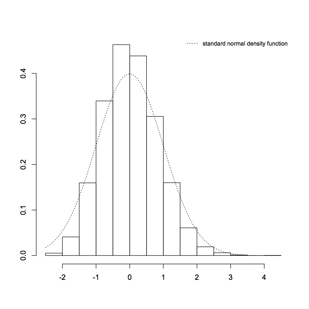
and we observe the L1L^{1}-convergence of f^t\hat{f}_{t} to the true density function ff of X0,0X_{0,0}. In order to illustrate the asymptotic normality of the estimator (8), we put x=−1x=-1, t=20t=20 and b20=0.7b_{20}=0.7 and we calculate the expectation 𝔼​(f^t​(−1))\mathbb{E}\left(\hat{f}_{t}(-1)\right) of f^t​(−1)\hat{f}_{t}(-1) by taking again the arithmetic mean value of 100100 replications of f^t​(−1)\hat{f}_{t}(-1). Finally, noting that ∫ℝK2​(x)​𝑑x=4/5\int_{\mathbb{R}}\textrm{K}^{2}(x)dx=4/5 and f⁡(−1)=1/100f(-1)=1/100, we consider 15001500 replications of

400×0.7​(f^20​(−1)−𝔼⁡(f^20​(−1)))1/100×4/5\frac{\sqrt{400\times 0.7}\left(\hat{f}_{20}(-1)-\mathbb{E}\left(\hat{f}_{20}(-1)\right)\right)}{\sqrt{1/100\times 4/5}}

and we obtain the following histogram (see figure 1) which seems to fit well to the target distribution, that is the standard normal law 𝒩⁡(0,1)\mathcal{N}(0,1).

Refer to caption
Figure 1: Asymptotic normality of the kernel density estimator.

In the simulation given in Figure 1, we fixed the bandwith b20=0.7b_{20}=0.7 arbitrarily since we do not investigate in this work any procedure for a data-driven choice of the bandwith parameter. Such a study is an important task and will be done in a forthcoming paper.

3 Proofs

The proof of all lemmas of this section are postponed to the appendix. In the sequel, the letter κ\kappa denotes a positive constant which the value is not important.

3.1 Proof of Theorem 1

For all positive integer nn, denote Jn=∫ℝ|fn​(x)−f⁡(x)|​𝑑x\textrm{J}_{n}=\int_{\mathbb{R}}|f_{n}(x)-f(x)|\,dx. For all real A≥1A\geq 1, we have Jn=Jn,1​(A)+Jn,2​(A)\textrm{J}_{n}=\textrm{J}_{n,1}(A)+\textrm{J}_{n,2}(A) where

Jn,1​(A)=∫|x|>A|fn​(x)−f⁡(x)|​𝑑xandJn,2​(A)=∫|x|≤A|fn​(x)−f⁡(x)|​𝑑x.\textrm{J}_{n,1}(A)=\int_{|x|>A}|f_{n}(x)-f(x)|\,dx\quad\textrm{and}\quad\textrm{J}_{n,2}(A)=\int_{|x|\leq A}|f_{n}(x)-f(x)|\,dx.

Moreover

𝔼​Jn,1​(A)≤∫|x|>A𝔼​|fn​(x)|​𝑑x+1A2​∫ℝx2​f​(x)​𝑑x\mathbb{E}\textrm{J}_{n,1}(A)\leq\int_{|x|>A}\mathbb{E}|f_{n}(x)|dx+\frac{1}{A^{2}}\int_{\mathbb{R}}x^{2}f(x)dx

and

∫|x|>A𝔼​|fn​(x)|​𝑑x\displaystyle\int_{|x|>A}\mathbb{E}|f_{n}(x)|dx ≤∫|x|>A∫ℝ|K​(t)|​f​(x−bn​t)​𝑑t​𝑑x\displaystyle\leq\int_{|x|>A}\int_{\mathbb{R}}|\textrm{K}(t)|f(x-b_{n}t)dtdx
=∫|t|>A2|K​(t)|​∫|x|>Af⁡(x−bn​t)​𝑑x​𝑑t+∫|t|≤A2|K​(t)|​∫|x|>Af⁡(x−bn​t)​𝑑x​𝑑t\displaystyle=\int_{|t|>\frac{A}{2}}|\textrm{K}(t)|\int_{|x|>A}f(x-b_{n}t)dxdt+\int_{|t|\leq\frac{A}{2}}|\textrm{K}(t)|\int_{|x|>A}f(x-b_{n}t)dxdt
≤∫|t|>A2|K​(t)|​∫|y+bn​t|>Af⁡(y)​𝑑y​𝑑t+∫|t|≤A2|K​(t)|​∫|y|>A⁡(1−bn2)f⁡(y)​𝑑y​𝑑t\displaystyle\leq\int_{|t|>\frac{A}{2}}|\textrm{K}(t)|\int_{|y+b_{n}t|>A}f(y)dydt+\int_{|t|\leq\frac{A}{2}}|\textrm{K}(t)|\int_{|y|>A(1-\frac{b_{n}}{2})}f(y)dydt
≤4A2​∫ℝt2​|K​(t)|​𝑑t+4A2​∫ℝ|K​(t)|​𝑑t​∫ℝy2​f​(y)​𝑑y.\displaystyle\leq\frac{4}{A^{2}}\int_{\mathbb{R}}t^{2}|\textrm{K}(t)|dt+\frac{4}{A^{2}}\int_{\mathbb{R}}|\textrm{K}(t)|dt\int_{\mathbb{R}}y^{2}f(y)dy.

Consequently, we obtain

𝔼​Jn,1​(A)≤κA2.\mathbb{E}\textrm{J}_{n,1}(A)\leq\frac{\kappa}{A^{2}}. (9)

Now, Jn,2​(A)≤Jn,2(1)​(A)+Jn,2(2)​(A)\textrm{J}_{n,2}(A)\leq\textrm{J}_{n,2}^{(1)}(A)+\textrm{J}_{n,2}^{(2)}(A) where

Jn,2(1)​(A)=∫|x|≤A|fn​(x)−𝔼​fn​(x)|​𝑑xandJn,2(2)​(A)=∫|x|≤A|𝔼​fn​(x)−f⁡(x)|​𝑑x.\textrm{J}_{n,2}^{(1)}(A)=\int_{|x|\leq A}|f_{n}(x)-\mathbb{E}f_{n}(x)|\,dx\quad\textrm{and}\quad\textrm{J}_{n,2}^{(2)}(A)=\int_{|x|\leq A}|\mathbb{E}f_{n}(x)-f(x)|\,dx.

Since

|𝔼​fn​(x)−f⁡(x)|\displaystyle|\mathbb{E}f_{n}(x)-f(x)| =|∫ℝK​(t)​(f⁡(x−bn​t)−f⁡(x))​𝑑t|\displaystyle=\left|\int_{\mathbb{R}}\textrm{K}(t)\left(f(x-b_{n}t)-f(x)\right)dt\right|
≤∫ℝ|K​(t)|​|f⁡(x−bn​t)−f⁡(x)|​𝑑t\displaystyle\leq\int_{\mathbb{R}}|\textrm{K}(t)|\left|f(x-b_{n}t)-f(x)\right|dt
≤κ​bn​∫ℝ|t|​|K​(t)|​𝑑t,\displaystyle\leq\kappa b_{n}\int_{\mathbb{R}}|t||\textrm{K}(t)|dt,

we obtain

Jn,2(2)​(A)≤κ​A​bn.\textrm{J}_{n,2}^{(2)}(A)\leq\kappa Ab_{n}. (10)

Keeping in mind the notation (4) and denoting f¯n​(x)=1|Λn|​bn​∑i∈ΛnK¯i​(x)\overline{f}_{n}(x)=\frac{1}{|\Lambda_{n}|b_{n}}\sum_{i\in\Lambda_{n}}\overline{\text{K}}_{i}(x), we have Jn,2(1)​(A)≤In,1​(A)+In,2​(A)\textrm{J}_{n,2}^{(1)}(A)\leq\text{I}_{n,1}(A)+\text{I}_{n,2}(A) where

In,1​(A)=∫|x|≤A|fn​(x)−f¯n​(x)|​𝑑xandIn,2​(A)=∫|x|≤A|f¯n​(x)−𝔼​f¯n​(x)|​𝑑x.\text{I}_{n,1}(A)=\int_{|x|\leq A}|f_{n}(x)-\overline{f}_{n}(x)|\,dx\quad\textrm{and}\quad\text{I}_{n,2}(A)=\int_{|x|\leq A}|\overline{f}_{n}(x)-\mathbb{E}\overline{f}_{n}(x)|\,dx.

By Lemma 2, we have

‖fn​(x)−f¯n​(x)‖2≤κ​∑|i|>mn|i|5​d2​δi|Λn|​bn​(mnd​bn)3/2.\left\|f_{n}(x)-\overline{f}_{n}(x)\right\|_{2}\leq\frac{\kappa\sum_{|i|>m_{n}}|i|^{\frac{5d}{2}}\delta_{i}}{\sqrt{|\Lambda_{n}|b_{n}}(m_{n}^{d}b_{n})^{3/2}}.

Applying Lemma 1, we obtain

𝔼​In,1​(A)≤κ​A|Λn|​bn.\mathbb{E}\text{I}_{n,1}(A)\leq\frac{\kappa A}{\sqrt{|\Lambda_{n}|b_{n}}}. (11)

Now, ‖f¯n​(x)−𝔼​f¯n​(x)‖22\left\|\overline{f}_{n}(x)-\mathbb{E}\overline{f}_{n}(x)\right\|_{2}^{2} equals to

1|Λn|2​bn​(|Λn|​𝔼​(Z¯02​(x))+∑j∈ℤd\{0}|j|<Mn|Λn∩(Λn−j)|​𝔼​(Z¯0​(x)​Z¯j​(x)))\frac{1}{|\Lambda_{n}|^{2}b_{n}}\left(|\Lambda_{n}|\mathbb{E}\left(\overline{Z}_{0}^{2}(x)\right)+\sum_{\begin{subarray}{c}j\in\mathbb{Z}^{d}\backslash\{0\}\\ |j|<M_{n}\end{subarray}}|\Lambda_{n}\cap(\Lambda_{n}-j)|\mathbb{E}\left(\overline{Z}_{0}(x)\overline{Z}_{j}(x)\right)\right) (12)

where we recall that Z¯i​(x)=1bn​(K¯i​(x)−𝔼​K¯i​(x))\overline{Z}_{i}(x)=\frac{1}{\sqrt{b_{n}}}\left(\overline{\text{K}}_{i}(x)-\mathbb{E}\overline{\text{K}}_{i}(x)\right) and Mn=2​mn+1M_{n}=2m_{n}+1.

Lemma 3

Let xx, ss and tt be fixed in ℝ\mathbb{R}. Then 𝔼⁡(Z¯02​(x))\mathbb{E}\left(\overline{Z}_{0}^{2}(x)\right) converges to f⁡(x)​∫ℝK2​(u)​𝑑uf(x)\int_{\mathbb{R}}\emph{\text{K}}^{2}(u)du and supi∈ℤd\{0}𝔼​|Z¯0​(s)​Z¯i​(t)|=o⁡(Mn−d)\sup_{i\in\mathbb{Z}^{d}\backslash\{0\}}\mathbb{E}|\overline{Z}_{0}(s)\overline{Z}_{i}(t)|=o(M_{n}^{-d}).

Combining (12) and Lemma 3, we derive ‖f¯n​(x)−𝔼​f¯n​(x)‖22=O⁡((|Λn|​bn)−1)\left\|\overline{f}_{n}(x)-\mathbb{E}\overline{f}_{n}(x)\right\|_{2}^{2}=O\left(\left(|\Lambda_{n}|b_{n}\right)^{-1}\right). Hence,

𝔼​In,2​(A)≤κ​A|Λn|​bn.\mathbb{E}\text{I}_{n,2}(A)\leq\frac{\kappa A}{\sqrt{|\Lambda_{n}|b_{n}}}. (13)

Combining (9), (10), (11) and (13), we obtain

𝔼​Jn≤κ⁡(1A2+A⁡(bn+1|Λn|​bn)).\mathbb{E}\textrm{J}_{n}\leq\kappa\left(\frac{1}{A^{2}}+A\left(b_{n}+\frac{1}{\sqrt{|\Lambda_{n}|b_{n}}}\right)\right).

Optimizing in AA, we derive (2). The proof of Theorem 1 is complete.

3.2 Proof of Theorem 2

Without loss of generality, we consider only the case k=2k=2 and we refer to x1x_{1} and x2x_{2} as xx and yy (x≠yx\neq y). Let λ1\lambda_{1} and λ2\lambda_{2} be two constants such that λ12+λ22=1\lambda_{1}^{2}+\lambda_{2}^{2}=1 and note that

λ1​(|Λn|​bn)1/2​(fn​(x)−𝔼​fn​(x))+λ2​(|Λn|​bn)1/2​(fn​(y)−𝔼​fn​(y))\displaystyle\lambda_{1}(|\Lambda_{n}|b_{n})^{1/2}(f_{n}(x)-\mathbb{E}f_{n}(x))+\lambda_{2}(|\Lambda_{n}|b_{n})^{1/2}(f_{n}(y)-\mathbb{E}f_{n}(y)) =∑i∈ΛnΔi|Λn|1/2,\displaystyle=\sum_{i\in\Lambda_{n}}\frac{\Delta_{i}}{|\Lambda_{n}|^{1/2}},
λ1​(|Λn|​bn)1/2​(f¯n​(x)−𝔼​f¯n​(x))+λ2​(|Λn|​bn)1/2​(f¯n​(y)−𝔼​f¯n​(y))\displaystyle\lambda_{1}(|\Lambda_{n}|b_{n})^{1/2}(\overline{f}_{n}(x)-\mathbb{E}\overline{f}_{n}(x))+\lambda_{2}(|\Lambda_{n}|b_{n})^{1/2}(\overline{f}_{n}(y)-\mathbb{E}\overline{f}_{n}(y)) =∑i∈ΛnΔ¯i|Λn|1/2,\displaystyle=\sum_{i\in\Lambda_{n}}\frac{\overline{\Delta}_{i}}{|\Lambda_{n}|^{1/2}},

where Δi=λ1​Zi​(x)+λ2​Zi​(y)\Delta_{i}=\lambda_{1}Z_{i}(x)+\lambda_{2}Z_{i}(y) and Δ¯i=λ1​Z¯i​(x)+λ2​Z¯i​(y)\overline{\Delta}_{i}=\lambda_{1}\overline{Z}_{i}(x)+\lambda_{2}\overline{Z}_{i}(y) and for all zz in ℝ\mathbb{R},

Zi​(z)=1bn​(Ki​(z)−𝔼​Ki​(z))andZ¯i​(z)=1bn​(K¯i​(z)−𝔼​K¯i​(z))Z_{i}(z)=\frac{1}{\sqrt{b_{n}}}\left(\text{K}_{i}(z)-\mathbb{E}\text{K}_{i}(z)\right)\quad\textrm{and}\quad\overline{Z}_{i}(z)=\frac{1}{\sqrt{b_{n}}}\left(\overline{\text{K}}_{i}(z)-\mathbb{E}\overline{\text{K}}_{i}(z)\right)

where Ki​(z)\text{K}_{i}(z) and K¯i​(z)\overline{\text{K}}_{i}(z) are defined by (4)(\ref{definition_K_i_z_overline_K_i_z}). Applying Lemma 1 and Lemma 2, we know that

1|Λn|1/2​‖∑i∈Λn(Δi−Δ¯i)‖2≤κ⁡(|λ1|+|λ2|)(mnd​bn)3/2​∑|i|>mn|i|5​d2​δi=o⁡(1).\frac{1}{|\Lambda_{n}|^{1/2}}\left\|\sum_{i\in\Lambda_{n}}\left(\Delta_{i}-\overline{\Delta}_{i}\right)\right\|_{2}\leq\frac{\kappa(|\lambda_{1}|+|\lambda_{2}|)}{(m_{n}^{d}b_{n})^{3/2}}\sum_{|i|>m_{n}}|i|^{\frac{5d}{2}}\delta_{i}=o(1). (14)

So, it suffices to prove the asymptotic normality of the sequence (|Λn|−1/2∑i∈ΛnΔ¯i)n≥1\left(|\Lambda_{n}|^{-1/2}\sum_{i\in\Lambda_{n}}\overline{\Delta}_{i}\right)_{n\geq 1}. We are going to follow the Lindeberg’s type proof of Theorem 11 in [8]. We consider the notations

η=(λ12​f​(x)+λ22​f​(y))​σ2andσ2=∫ℝK2​(u)​𝑑u.\eta=(\lambda_{1}^{2}f(x)+\lambda_{2}^{2}f(y))\sigma^{2}\quad\textrm{and}\quad\sigma^{2}=\int_{\mathbb{R}}\text{K}^{2}(u)du. (15)
Lemma 4

𝔼⁡(Δ¯02)\mathbb{E}(\overline{\Delta}_{0}^{2}) converges to η\eta and supi∈ℤd\{0}𝔼​|Δ¯0​Δ¯i|=o⁡(Mn−d)\sup_{i\in\mathbb{Z}^{d}\backslash\{0\}}\mathbb{E}|\overline{\Delta}_{0}\overline{\Delta}_{i}|=o(M_{n}^{-d}).

On the lattice ℤd\mathbb{Z}^{d} we define the lexicographic order as follows: if i=(i1,…,id)i=(i_{1},...,i_{d}) and j=(j1,…,jd)j=(j_{1},...,j_{d}) are distinct elements of ℤd\mathbb{Z}^{d}, the notation i<lexji<_{\textrm{lex}}j means that either i1<j1i_{1}<j_{1} or for some kk in {2,3,…,d}\{2,3,...,d\}, ik<jki_{k}<j_{k} and il=jli_{l}=j_{l} for 1≤l<k1\leq l<k. We let φ\varphi denote the unique function from {1,…,|Λn|}\{1,...,|\Lambda_{n}|\} to Λn\Lambda_{n} such that φ(k)<lexφ(l)\varphi(k)<_{\text{\text{lex}}}\varphi(l) for 1≤k<l≤|Λn|1\leq k<l\leq|\Lambda_{n}|. For all real random field (ζi)i∈ℤd(\zeta_{i})_{i\in\mathbb{Z}^{d}} and all integer kk in {1,…,|Λn|}\{1,...,|\Lambda_{n}|\}, we denote

Sφ⁡(k)​(ζ)=∑i=1kζφ⁡(i)andSφ⁡(k)c​(ζ)=∑i=k|Λn|ζφ⁡(i)S_{\varphi(k)}(\zeta)=\sum_{i=1}^{k}\zeta_{\varphi(i)}\quad\textrm{and}\quad S_{\varphi(k)}^{c}(\zeta)=\sum_{i=k}^{|\Lambda_{n}|}\zeta_{\varphi(i)}

with the convention Sφ⁡(0)​(ζ)=Sφ⁡(|Λn|+1)c​(ζ)=0S_{\varphi(0)}(\zeta)=S_{\varphi(|\Lambda_{n}|+1)}^{c}(\zeta)=0. From now on, we consider a field (ξi)i∈ℤd(\xi_{i})_{i\in\mathbb{Z}^{d}} of i.i.d. standard normal random variables independent of (Xi)i∈ℤd(X_{i})_{i\in\mathbb{Z}^{d}}. We introduce the fields YY and γ\gamma defined for all ii in ℤd\mathbb{Z}^{d} by

Yi=Δ¯i|Λn|1/2andγi=η​ξi|Λn|1/2Y_{i}=\frac{\overline{\Delta}_{i}}{|\Lambda_{n}|^{1/2}}\quad\textrm{and}\quad\gamma_{i}=\frac{\sqrt{\eta}\xi_{i}}{|\Lambda_{n}|^{1/2}}

where η\eta is defined by (15). Note that YY is an MnM_{n}-dependent random field where Mn=2​mn+1M_{n}=2m_{n}+1 and mnm_{n} is defined by (3). Let hh be any function from ℝ\mathbb{R} to ℝ\mathbb{R}. For 0<k≤l≤|Λn|0<k\leq l\leq|\Lambda_{n}|, we introduce hk,l​(Y)=h⁡(Sφ⁡(k)​(Y)+Sφ⁡(l)c​(γ))h_{k,l}(Y)=h(S_{\varphi(k)}(Y)+S_{\varphi(l)}^{c}(\gamma)). With the above convention we have that hk,|Λn|+1​(Y)=h⁡(Sφ⁡(k)​(Y))h_{k,|\Lambda_{n}|+1}(Y)=h(S_{\varphi(k)}(Y)) and also h0,l​(Y)=h⁡(Sφ⁡(l)c​(γ))h_{0,l}(Y)=h(S_{\varphi(l)}^{c}(\gamma)). In the sequel, we will often write hk,lh_{k,l} instead of hk,l​(Y)h_{k,l}(Y). We denote by B14​(ℝ)B_{1}^{4}(\mathbb{R}) the unit ball of Cb4​(ℝ)C_{b}^{4}(\mathbb{R}): hh belongs to B14​(ℝ)B_{1}^{4}(\mathbb{R}) if and only if it belongs to C4​(ℝ)C^{4}(\mathbb{R}) and satisfies max0≤i≤4⁡‖h(i)‖∞≤1\max_{0\leq i\leq 4}\|h^{(i)}\|_{\infty}\leq 1. It suffices to prove that for all hh in B14​(ℝ)B_{1}^{4}(\mathbb{R}),

𝔼⁡(h⁡(Sφ⁡(|Λn|)​(Y)))→n→∞𝔼⁡(h⁡(η​ξ0)).\mathbb{E}\left(h\left(S_{\varphi(|\Lambda_{n}|)}(Y)\right)\right)\mathrel{\mathop{\kern 0.0pt\hbox to42.67912pt{\rightarrowfill}}\limits_{n\rightarrow\infty}^{\hbox{\scriptsize}}}\mathbb{E}\left(h\left(\sqrt{\eta}\xi_{0}\right)\right).

We use Lindeberg’s decomposition:

𝔼⁡(h⁡(Sφ⁡(|Λn|)​(Y))−h⁡(η​ξ0))=∑k=1|Λn|𝔼⁡(hk,k+1−hk−1,k).\mathbb{E}\left(h\left(S_{\varphi(|\Lambda_{n}|)}(Y)\right)-h\left(\sqrt{\eta}\xi_{0}\right)\right)=\sum_{k=1}^{|\Lambda_{n}|}\mathbb{E}\left(h_{k,k+1}-h_{k-1,k}\right).

Now, we have hk,k+1−hk−1,k=hk,k+1−hk−1,k+1+hk−1,k+1−hk−1,kh_{k,k+1}-h_{k-1,k}=h_{k,k+1}-h_{k-1,k+1}+h_{k-1,k+1}-h_{k-1,k} and by Taylor’s formula we obtain

hk,k+1−hk−1,k+1\displaystyle h_{k,k+1}-h_{k-1,k+1} =Yφ⁡(k)hk−1,k+1′+12Yφ⁡(k)2hk−1,k+1′′+Rk\displaystyle=Y_{\varphi(k)}h_{k-1,k+1}^{{}^{\prime}}+\frac{1}{2}Y_{\varphi(k)}^{2}h_{k-1,k+1}^{{}^{\prime\prime}}+R_{k}
hk−1,k+1−hk−1,k\displaystyle h_{k-1,k+1}-h_{k-1,k} =−γφ⁡(k)hk−1,k+1′−12γφ⁡(k)2hk−1,k+1′′+rk\displaystyle=-\gamma_{\varphi(k)}h_{k-1,k+1}^{{}^{\prime}}-\frac{1}{2}\gamma_{\varphi(k)}^{2}h_{k-1,k+1}^{{}^{\prime\prime}}+r_{k}

where |Rk|≤Yφ⁡(k)2​(1∧|Yφ⁡(k)|)|R_{k}|\leq Y_{\varphi(k)}^{2}(1\wedge|Y_{\varphi(k)}|) and |rk|≤γφ⁡(k)2​(1∧|γφ⁡(k)|)|r_{k}|\leq\gamma_{\varphi(k)}^{2}(1\wedge|\gamma_{\varphi(k)}|). Since (Y,ξi)i≠φ⁡(k)(Y,\xi_{i})_{i\neq\varphi(k)} is independent of ξφ⁡(k)\xi_{\varphi(k)}, it follows that

𝔼(γφ⁡(k)hk−1,k+1′)=0and𝔼(γφ⁡(k)2hk−1,k+1′′)=𝔼(η|Λn|hk−1,k+1′′)\mathbb{E}\left(\gamma_{\varphi(k)}h_{k-1,k+1}^{{}^{\prime}}\right)=0\quad\textrm{and}\quad\mathbb{E}\left(\gamma_{\varphi(k)}^{2}h_{k-1,k+1}^{{}^{\prime\prime}}\right)=\mathbb{E}\left(\frac{\eta}{|\Lambda_{n}|}h_{k-1,k+1}^{{}^{\prime\prime}}\right)

Hence, we obtain

𝔼⁡(h⁡(Sφ⁡(|Λn|)​(Y))−h⁡(η​ξ0))\displaystyle\mathbb{E}\left(h(S_{\varphi(|\Lambda_{n}|)}(Y))-h\left(\sqrt{\eta}\xi_{0}\right)\right) =∑k=1|Λn|𝔼(Yφ⁡(k)hk−1,k+1′)\displaystyle=\sum_{k=1}^{|\Lambda_{n}|}\mathbb{E}(Y_{\varphi(k)}h_{k-1,k+1}^{{}^{\prime}})
+∑k=1|Λn|𝔼((Yφ⁡(k)2−η|Λn|)hk−1,k+1′′2)\displaystyle\quad+\sum_{k=1}^{|\Lambda_{n}|}\mathbb{E}\left(\left(Y_{\varphi(k)}^{2}-\frac{\eta}{|\Lambda_{n}|}\right)\frac{h_{k-1,k+1}^{{}^{\prime\prime}}}{2}\right)
+∑k=1|Λn|𝔼(Rk+rk).\displaystyle\quad+\sum_{k=1}^{|\Lambda_{n}|}\mathbb{E}\left(R_{k}+r_{k}\right).

Let 1≤k≤|Λn|1\leq k\leq|\Lambda_{n}| be fixed. Since 𝔼​|Δ¯0|=O⁡(bn)\mathbb{E}|\overline{\Delta}_{0}|=O\left(\sqrt{b_{n}}\right) and (Δ¯02​bn)n≥1\left(\overline{\Delta}_{0}^{2}b_{n}\right)_{n\geq 1} is uniformly integrable, we derive

∑k=1|Λn|𝔼​|Rk|≤𝔼⁡(Δ¯02​(1∧|Δ¯0||Λn|1/2))=o⁡(1)\sum_{k=1}^{|\Lambda_{n}|}\mathbb{E}|R_{k}|\leq\mathbb{E}\left(\overline{\Delta}_{0}^{2}\left(1\wedge\frac{|\overline{\Delta}_{0}|}{|\Lambda_{n}|^{1/2}}\right)\right)=o(1)

and

∑k=1|Λn|𝔼|rk|≤η3/2​𝔼​|ξ0|3|Λn|1/2=O(|Λn|−1/2).\sum_{k=1}^{|\Lambda_{n}|}\mathbb{E}|r_{k}|\leq\frac{\eta^{3/2}\mathbb{E}|\xi_{0}|^{3}}{|\Lambda_{n}|^{1/2}}=O\left(|\Lambda_{n}|^{-1/2}\right).

Consequently, we obtain

∑k=1|Λn|𝔼⁡(|Rk|+|rk|)=o⁡(1).\sum_{k=1}^{|\Lambda_{n}|}\mathbb{E}\left(|R_{k}|+|r_{k}|\right)=o(1).

Now, it is sufficient to show

limn→∞∑k=1|Λn|(𝔼(Yφ⁡(k)hk−1,k+1′)+𝔼((Yφ⁡(k)2−η|Λn|)hk−1,k+1′′2))=0.\lim_{n\to\infty}\sum_{k=1}^{|\Lambda_{n}|}\left(\mathbb{E}(Y_{\varphi(k)}h_{k-1,k+1}^{{}^{\prime}})+\mathbb{E}\left(\left(Y_{\varphi(k)}^{2}-\frac{\eta}{|\Lambda_{n}|}\right)\frac{h_{k-1,k+1}^{{}^{\prime\prime}}}{2}\right)\right)=0. (16)

First, we focus on ∑k=1|Λn|𝔼(Yφ⁡(k)hk−1,k+1′)\sum_{k=1}^{|\Lambda_{n}|}\mathbb{E}\left(Y_{\varphi(k)}h_{k-1,k+1}^{{}^{\prime}}\right). Let the sets {Vik;i∈ℤd,k∈ℕ\{0}}\{V_{i}^{k}\,;\,i\in\mathbb{Z}^{d}\,,\,k\in\mathbb{N}\backslash\{0\}\} be defined as follows: Vi1={j∈ℤd;j<lexi}V_{i}^{1}=\{j\in\mathbb{Z}^{d}\,;\,j<_{\textrm{lex}}i\} and for k≥2k\geq 2, Vik=Vi1∩{j∈ℤd;|i−j|≥k}V_{i}^{k}=V_{i}^{1}\cap\{j\in\mathbb{Z}^{d}\,;\,|i-j|\geq k\}. For all nn in ℕ\{0}\mathbb{N}\backslash\{0\} and all kk in {1,…,|Λn|}\{1,...,|\Lambda_{n}|\}, we define

Ek(n)=φ({1,..,k})∩Vφ⁡(k)MnandSφ⁡(k)Mn(Y)=∑i∈Ek(n)Yi.\textrm{E}_{k}^{(n)}=\varphi(\{1,..,k\})\cap V_{\varphi(k)}^{M_{n}}\quad\textrm{and}\quad S_{\varphi(k)}^{M_{n}}(Y)=\sum_{i\in\textrm{E}_{k}^{(n)}}Y_{i}.

For all function hh from ℝ\mathbb{R} to ℝ\mathbb{R}, we define hk−1,lMn=h⁡(Sφ⁡(k)Mn​(Y)+Sφ⁡(l)c​(γ))h_{k-1,l}^{M_{n}}=h\left(S_{\varphi(k)}^{M_{n}}(Y)+S_{\varphi(l)}^{c}(\gamma)\right). Our aim is to show that

limn→∞∑k=1|Λn|𝔼(Yφ⁡(k)hk−1,k+1′−Yφ⁡(k)(Sφ⁡(k−1)(Y)−Sφ⁡(k)Mn(Y))hk−1,k+1′′)=0.\lim_{n\to\infty}\sum_{k=1}^{|\Lambda_{n}|}\mathbb{E}\left(Y_{\varphi(k)}h_{k-1,k+1}^{{}^{\prime}}-Y_{\varphi(k)}\left(S_{\varphi(k-1)}(Y)-S_{\varphi(k)}^{M_{n}}(Y)\right)h_{k-1,k+1}^{{}^{\prime\prime}}\right)=0. (17)

First, we use the decomposition

Yφ⁡(k)hk−1,k+1′=Yφ⁡(k)hk−1,k+1Mn′+Yφ⁡(k)(hk−1,k+1′−hk−1,k+1Mn′).Y_{\varphi(k)}h_{k-1,k+1}^{{}^{\prime}}=Y_{\varphi(k)}h_{k-1,k+1}^{{}^{\prime}M_{n}}+Y_{\varphi(k)}\left(h_{k-1,k+1}^{{}^{\prime}}-h_{k-1,k+1}^{{}^{\prime}M_{n}}\right).

Applying again Taylor’s formula,

Yφ⁡(k)(hk−1,k+1′−hk−1,k+1Mn′)=Yφ⁡(k)(Sφ⁡(k−1)(Y)−Sφ⁡(k)Mn(Y))hk−1,k+1′′+Rk′,Y_{\varphi(k)}(h_{k-1,k+1}^{{}^{\prime}}-h_{k-1,k+1}^{{}^{\prime}M_{n}})=Y_{\varphi(k)}\left(S_{\varphi(k-1)}(Y)-S_{\varphi(k)}^{M_{n}}(Y)\right)h_{k-1,k+1}^{{}^{\prime\prime}}+R_{k}^{{}^{\prime}},

where

|Rk′|≤2|Yφ⁡(k)(Sφ⁡(k−1)(Y)−Sφ⁡(k)Mn(Y))(1∧|Sφ⁡(k−1)(Y)−Sφ⁡(k)Mn(Y)|)|.|R_{k}^{{}^{\prime}}|\leq 2\left|Y_{\varphi(k)}\left(S_{\varphi(k-1)}(Y)-S_{\varphi(k)}^{M_{n}}(Y)\right)\left(1\wedge|S_{\varphi(k-1)}(Y)-S_{\varphi(k)}^{M_{n}}(Y)|\right)\right|.

Since (Yi)i∈ℤd(Y_{i})_{i\in\mathbb{Z}^{d}} is MnM_{n}-dependent, we have 𝔼⁡(Yφ⁡(k)​hk−1,k+1Mn′)=0\mathbb{E}\left(Y_{\varphi(k)}h_{k-1,k+1}^{{}^{\prime}{M_{n}}}\right)=0 and consequently (17)(\ref{equation1bis}) holds if and only if limn→∞∑k=1|Λn|𝔼|Rk′|=0\lim_{n\to\infty}\sum_{k=1}^{|\Lambda_{n}|}\mathbb{E}|R_{k}^{{}^{\prime}}|=0. In fact, considering the sets Wn={−Mn+1,…,Mn−1}dW_{n}=\{-M_{n}+1,...,M_{n}-1\}^{d} and Wn∗=Wn\{0}W_{n}^{\ast}=W_{n}\backslash\{0\}, it follows that

∑k=1|Λn|𝔼|Rk′|\displaystyle\sum_{k=1}^{|\Lambda_{n}|}\mathbb{E}|R_{k}^{{}^{\prime}}| ≤2​𝔼​(|Δ¯0|​(∑i∈Wn∗|Δ¯i|)​(1∧1|Λn|1/2​∑i∈Wn∗|Δ¯i|))\displaystyle\leq 2\mathbb{E}\left(|\overline{\Delta}_{0}|\left(\sum_{i\in W_{n}^{\ast}}|\overline{\Delta}_{i}|\right)\left(1\wedge\frac{1}{|\Lambda_{n}|^{1/2}}\sum_{i\in W_{n}^{\ast}}|\overline{\Delta}_{i}|\right)\right)
≤2​Mnd​supi∈ℤd\{0}𝔼⁡(|Δ¯0​Δ¯i|)\displaystyle\leq 2M_{n}^{d}\sup_{i\in\mathbb{Z}^{d}\backslash\{0\}}\mathbb{E}(|\overline{\Delta}_{0}\overline{\Delta}_{i}|)
=o(1)(by Lemma 4).\displaystyle=o(1)\qquad\textrm{(by Lemma \ref{lemme-technique})}.

In order to obtain (16) it remains to control

F1=𝔼(∑k=1|Λn|hk−1,k+1′′(Yφ⁡(k)22+Yφ⁡(k)(Sφ⁡(k−1)(Y)−Sφ⁡(k)Mn(Y))−η2​|Λn|)).\textrm{F}_{1}=\mathbb{E}\left(\sum_{k=1}^{|\Lambda_{n}|}h_{k-1,k+1}^{{}^{\prime\prime}}\left(\frac{Y_{\varphi(k)}^{2}}{2}+Y_{\varphi(k)}\left(S_{\varphi(k-1)}(Y)-S_{\varphi(k)}^{M_{n}}(Y)\right)-\frac{\eta}{2|\Lambda_{n}|}\right)\right).

Applying again Lemma 4, we have

F1\displaystyle\textrm{F}_{1} ≤|𝔼(1|Λn|∑k=1|Λn|hk−1,k+1′′(Δ¯φ⁡(k)2−𝔼(Δ¯02)))|+|η−𝔼(Δ¯02)|+2∑j∈V01∩Wn𝔼|Δ¯0Δ¯j|\displaystyle\leq\left|\mathbb{E}\left(\frac{1}{|\Lambda_{n}|}\sum_{k=1}^{|\Lambda_{n}|}h_{k-1,k+1}^{{}^{\prime\prime}}\left(\overline{\Delta}_{\varphi(k)}^{2}-\mathbb{E}(\overline{\Delta}_{0}^{2})\right)\right)\right|+\left|\eta-\mathbb{E}\left(\overline{\Delta}_{0}^{2}\right)\right|+2\sum_{j\in V_{0}^{1}\cap W_{n}}\mathbb{E}|\overline{\Delta}_{0}\overline{\Delta}_{j}|
≤|𝔼(1|Λn|∑k=1|Λn|hk−1,k+1′′(Δ¯φ⁡(k)2−𝔼(Δ¯02)))|+o(1).\displaystyle\leq\left|\mathbb{E}\left(\frac{1}{|\Lambda_{n}|}\sum_{k=1}^{|\Lambda_{n}|}h_{k-1,k+1}^{{}^{\prime\prime}}\left(\overline{\Delta}_{\varphi(k)}^{2}-\mathbb{E}(\overline{\Delta}_{0}^{2})\right)\right)\right|+o(1).

So, it suffices to prove that

F2=|𝔼(1|Λn|∑k=1|Λn|hk−1,k+1′′(Δ¯φ⁡(k)2−𝔼(Δ¯02)))|\textrm{F}_{2}=\left|\mathbb{E}\left(\frac{1}{|\Lambda_{n}|}\sum_{k=1}^{|\Lambda_{n}|}h_{k-1,k+1}^{{}^{\prime\prime}}\left(\overline{\Delta}_{\varphi(k)}^{2}-\mathbb{E}(\overline{\Delta}_{0}^{2})\right)\right)\right|

goes to zero as nn goes to infinity. In fact, we have F2≤1|Λn|​∑k=1|Λn|(Jk(1)​(n)+Jk(2)​(n))\textrm{F}_{2}\leq\frac{1}{|\Lambda_{n}|}\sum_{k=1}^{|\Lambda_{n}|}\left(\textrm{J}_{k}^{(1)}(n)+\textrm{J}_{k}^{(2)}(n)\right) where Jk(1)​(n)=|𝔼⁡(hk−1,k+1Mn′′​(Δ¯φ⁡(k)2−𝔼⁡(Δ¯02)))|=0\textrm{J}_{k}^{(1)}(n)=\left|\mathbb{E}\left(h_{k-1,k+1}^{{}^{\prime\prime}M_{n}}\left(\overline{\Delta}_{\varphi(k)}^{2}-\mathbb{E}\left(\overline{\Delta}_{0}^{2}\right)\right)\right)\right|=0 since hk−1,k+1Mn′′h_{k-1,k+1}^{{}^{\prime\prime}M_{n}} and Δ¯φ⁡(k)\overline{\Delta}_{\varphi(k)} are independent. Moreover,

Jk(2)​(n)\displaystyle\textrm{J}_{k}^{(2)}(n) =|𝔼((hk−1,k+1′′−hk−1,k+1Mn′′)(Δ¯φ⁡(k)2−𝔼(Δ¯02)))|\displaystyle=\left|\mathbb{E}\left(\left(h_{k-1,k+1}^{{}^{\prime\prime}}-h_{k-1,k+1}^{{}^{\prime\prime}M_{n}}\right)\left(\overline{\Delta}_{\varphi(k)}^{2}-\mathbb{E}\left(\overline{\Delta}_{0}^{2}\right)\right)\right)\right|
≤𝔼⁡((2∧∑|i|<Mni≠0|Δ¯i||Λn|1/2)​Δ¯02)\displaystyle\leq\mathbb{E}\left(\left(2\wedge\sum_{\begin{subarray}{c}|i|<M_{n}\\ i\neq 0\end{subarray}}\frac{|\overline{\Delta}_{i}|}{|\Lambda_{n}|^{1/2}}\right)\overline{\Delta}_{0}^{2}\right)
≤1|Λn|​bn​𝔼​(|Δ¯0|​bn×∑|i|<Mni≠0|Δ¯0​Δ¯i|)\displaystyle\leq\frac{1}{\sqrt{|\Lambda_{n}|b_{n}}}\,\mathbb{E}\left(|\overline{\Delta}_{0}|\sqrt{b_{n}}\times\sum_{\begin{subarray}{c}|i|<M_{n}\\ i\neq 0\end{subarray}}|\overline{\Delta}_{0}\overline{\Delta}_{i}|\right)
=o⁡(1)\displaystyle=o(1)

since (|Δ¯0|​bn)n≥1(|\overline{\Delta}_{0}|\sqrt{b_{n}})_{n\geq 1} is uniformly integrable and ∑|i|<Mni≠0𝔼​|Δ¯0​Δ¯i|=o⁡(1)\sum_{\begin{subarray}{c}|i|<M_{n}\\ i\neq 0\end{subarray}}\mathbb{E}|\overline{\Delta}_{0}\overline{\Delta}_{i}|=o(1) by Lemma 4. The proof of Theorem 2 is complete.

3.3 Proof of Theorem 3

Let nn be a fixed positive integer and let xx be fixed in ℝ\mathbb{R}. We have Un​(x)=U¯n​(x)+Rn​(x)U_{n}(x)=\overline{U}_{n}(x)+R_{n}(x) where

U¯n​(x)=|Λn|​bn​(f¯n​(x)−𝔼​f¯n​(x))f⁡(x)​∫ℝK2​(t)​𝑑tandRn​(x)=|Λn|​bn​(fn​(x)−f¯n​(x))f⁡(x)​∫ℝK2​(t)​𝑑t.\overline{U}_{n}(x)=\frac{\sqrt{|\Lambda_{n}|b_{n}}\left(\overline{f}_{n}(x)-\mathbb{E}\overline{f}_{n}(x)\right)}{\sqrt{f(x)\int_{\mathbb{R}}\text{K}^{2}(t)dt}}\quad\textrm{and}\quad R_{n}(x)=\frac{\sqrt{|\Lambda_{n}|b_{n}}\left(f_{n}(x)-\overline{f}_{n}(x)\right)}{\sqrt{f(x)\int_{\mathbb{R}}\text{K}^{2}(t)dt}}.

Denote D¯n​(x)=supt∈ℝ|ℙ⁡(U¯n​(x)≤t)−Φ⁡(t)|\overline{D}_{n}(x)=\sup_{t\in\mathbb{R}}|\mathbb{P}(\overline{U}_{n}(x)\leq t)-\Phi(t)| and let p≥2p\geq 2 be fixed. Arguing as in Theorem 2.2 in [10], we have

Dn​(x)≤D¯n​(x)+‖Rn‖ppp+1.D_{n}(x)\leq\overline{D}_{n}(x)+\|R_{n}\|_{p}^{\frac{p}{p+1}}. (18)

Denoting σ2=f⁡(x)​∫ℝK2​(t)​𝑑t\sigma^{2}=f(x)\int_{\mathbb{R}}\text{K}^{2}(t)dt and σn2=𝔼⁡(U¯n2)\sigma_{n}^{2}=\mathbb{E}\left(\overline{U}_{n}^{2}\right), we have

D¯n​(x)\displaystyle\overline{D}_{n}(x) =supt∈ℝ|ℙ⁡(U¯n​(x)≤t)−Φ⁡(t)|\displaystyle=\sup_{t\in\mathbb{R}}|\mathbb{P}(\overline{U}_{n}(x)\leq t)-\Phi(t)|
≤supt∈ℝ|ℙ⁡(U¯n​(x)≤t)−Φ⁡(t/σn)|+supt∈ℝ|Φ⁡(t/σn)−Φ⁡(t)|\displaystyle\leq\sup_{t\in\mathbb{R}}|\mathbb{P}(\overline{U}_{n}(x)\leq t)-\Phi\left(t/\sigma_{n}\right)|+\sup_{t\in\mathbb{R}}|\Phi\left(t/\sigma_{n}\right)-\Phi\left(t\right)|
=supt∈ℝ|ℙ⁡(U¯n​(x)≤t​σn)−Φ⁡(t)|+supt∈ℝ|Φ⁡(t/σn)−Φ⁡(t)|.\displaystyle=\sup_{t\in\mathbb{R}}|\mathbb{P}(\overline{U}_{n}(x)\leq t\sigma_{n})-\Phi\left(t\right)|+\sup_{t\in\mathbb{R}}|\Phi\left(t/\sigma_{n}\right)-\Phi\left(t\right)|.

Applying the Berry-Esseen’s type theorem for mnm_{n}-dependent random fields established by Chen and Shao ([5], Theorem 2.6), we obtain

supt∈ℝ|ℙ⁡(U¯n​(x)≤t​σn)−Φ⁡(t)|≤κ​∫ℝ|K⁡(t)|τ​f​(x−t​bn)​𝑑t​mn(τ−1)​dστ​(|Λn|​bn)τ2−1.\sup_{t\in\mathbb{R}}|\mathbb{P}(\overline{U}_{n}(x)\leq t\sigma_{n})-\Phi\left(t\right)|\leq\frac{\kappa\int_{\mathbb{R}}|K(t)|^{\tau}f(x-tb_{n})dt\,\,m_{n}^{(\tau-1)d}}{\sigma^{\tau}(|\Lambda_{n}|b_{n})^{\frac{\tau}{2}-1}}. (19)

Arguing as in Yang et al. ([27], p. 456), we have

supt∈ℝ|Φ⁡(t/σn)−Φ⁡(t)|\displaystyle\sup_{t\in\mathbb{R}}|\Phi\left(t/\sigma_{n}\right)-\Phi\left(t\right)| ≤(2​π​e)−12​(σn−1)​1​1σn≥1+(2​π​e)−12​(1σn−1)​1​10<σn<1\displaystyle\leq(2\pi e)^{-\frac{1}{2}}(\sigma_{n}-1)\,\hbox to0.0pt{\mbox{\small\rm 1}\hss}\kern 1.49994pt1_{\sigma_{n}\geq 1}+(2\pi e)^{-\frac{1}{2}}\left(\frac{1}{\sigma_{n}}-1\right)\,\hbox to0.0pt{\mbox{\small\rm 1}\hss}\kern 1.49994pt1_{0<\sigma_{n}<1}
≤(2πe)−12max{|σn−1|,|σn−1|σn}}\displaystyle\leq(2\pi e)^{-\frac{1}{2}}\max\left\{|\sigma_{n}-1|,\frac{|\sigma_{n}-1|}{\sigma_{n}}\}\right\}
≤κmax{|σn−1|,|σn−1|σn}}×(σn+1)\displaystyle\leq\kappa\max\left\{|\sigma_{n}-1|,\frac{|\sigma_{n}-1|}{\sigma_{n}}\}\right\}\times(\sigma_{n}+1)
≤κ​|σn2−1|.\displaystyle\leq\kappa|\sigma_{n}^{2}-1|.

So, we derive

D¯n​(x)≤κ​∫ℝ|K⁡(t)|τ​f​(x−t​bn)​𝑑t​mn(τ−1)​dστ​(|Λn|​bn)τ2−1+κ​|σn2−1|.\overline{D}_{n}(x)\leq\frac{\kappa\int_{\mathbb{R}}|K(t)|^{\tau}f(x-tb_{n})dt\,\,m_{n}^{(\tau-1)d}}{\sigma^{\tau}(|\Lambda_{n}|b_{n})^{\frac{\tau}{2}-1}}+\kappa|\sigma_{n}^{2}-1|. (20)

Using (12), we have also

|σn2−1|≤1σ2​|𝔼⁡(Z¯02​(x))−σ2|+∑j∈ℤd\{0}|j|<Mn|𝔼⁡(Z¯0​(x)​Z¯j​(x))|.|\sigma_{n}^{2}-1|\leq\frac{1}{\sigma^{2}}\left|\mathbb{E}(\overline{Z}_{0}^{2}(x))-\sigma^{2}\right|+\sum_{\begin{subarray}{c}j\in\mathbb{Z}^{d}\backslash\{0\}\\ |j|<M_{n}\end{subarray}}\left|\mathbb{E}\left(\overline{Z}_{0}(x)\overline{Z}_{j}(x)\right)\right|. (21)

Noting that ‖K0​(x)‖1=O⁡(bn)\|\text{K}_{0}(x)\|_{1}=O(b_{n}) and ‖K0​(x)‖2=O⁡(bn)\|\text{K}_{0}(x)\|_{2}=O(\sqrt{b_{n}}) and using the following lemma,

Lemma 5

For all p>1p>1, any positive integer nn and any xx in ℝ\mathbb{R},

‖​K0​(x)−​K¯0​(x)‖p≤2​pbn​∑|j|>mnδj,p,\|\emph{K}_{0}(x)-\overline{\emph{K}}_{0}(x)\|_{p}\leq\frac{\sqrt{2p}}{b_{n}}\sum_{|j|>m_{n}}\delta_{j,p},

we obtain

|𝔼⁡(Z¯02​(x))−𝔼⁡(Z02​(x))|\displaystyle\left|\mathbb{E}(\overline{Z}_{0}^{2}(x))-\mathbb{E}(Z_{0}^{2}(x))\right| =1bn​|𝔼⁡(K¯02​(x))−𝔼⁡(K02​(x))|\displaystyle=\frac{1}{b_{n}}\left|\mathbb{E}(\overline{\text{K}}_{0}^{2}(x))-\mathbb{E}(\text{K}_{0}^{2}(x))\right|
≤1bn​‖K0​(x)‖2​‖K0​(x)−K¯0​(x)‖2\displaystyle\leq\frac{1}{b_{n}}\|\text{K}_{0}(x)\|_{2}\|\text{K}_{0}(x)-\overline{\text{K}}_{0}(x)\|_{2}
≤κbn3/2​∑|j|>mnδj\displaystyle\leq\frac{\kappa}{b_{n}^{3/2}}\sum_{|j|>m_{n}}\delta_{j}

and

|𝔼⁡(Z02​(x))−σ2|\displaystyle\left|\mathbb{E}(Z_{0}^{2}(x))-\sigma^{2}\right| =|1bn(𝔼(K02(x))−(𝔼(K0(x))2)−f(x)∫ℝK2(t)dt|\displaystyle=\left|\frac{1}{b_{n}}\left(\mathbb{E}(\text{K}_{0}^{2}(x))-\left(\mathbb{E}(\text{K}_{0}(x)\right)^{2}\right)-f(x)\int_{\mathbb{R}}\text{K}^{2}(t)dt\right|
≤|1bn​𝔼​(K02​(x))−f⁡(x)​∫ℝK2​(t)​𝑑t|+1bn​(𝔼​(K0​(x))2CLOSE\displaystyle\leq\left|\frac{1}{b_{n}}\mathbb{E}(\text{K}_{0}^{2}(x))-f(x)\int_{\mathbb{R}}\text{K}^{2}(t)dt\right|+\frac{1}{b_{n}}\left(\mathbb{E}(\text{K}_{0}(x)\right)^{2}
≤∫ℝK2​(v)|f⁡(x−v​bn)−f⁡(x)|𝑑v+O⁡(bn)\displaystyle\leq\int_{\mathbb{R}}\text{K}^{2}(v)|f(x-vb_{n})-f(x)|dv+O(b_{n})
≤κ​bn​∫ℝ|v|​K2​(v)​𝑑v+O⁡(bn)\displaystyle\leq\kappa\,b_{n}\int_{\mathbb{R}}|v|\text{K}^{2}(v)dv+O(b_{n})
=O⁡(bn).\displaystyle=O(b_{n}).

Hence,

|𝔼⁡(Z¯02​(x))−σ2|≤κbn3/2​∑|j|>mnδj+O⁡(bn).\left|\mathbb{E}(\overline{Z}_{0}^{2}(x))-\sigma^{2}\right|\leq\frac{\kappa}{b_{n}^{3/2}}\sum_{|j|>m_{n}}\delta_{j}+O(b_{n}). (22)

Now, let i≠0i\neq 0 be fixed. We have

𝔼​|Z¯0​(x)​Z¯i​(x)|≤1bn​𝔼​|K¯0​(x)​K¯i​(x)|+3bn​(𝔼​|K0​(x)|)2.\mathbb{E}|\overline{Z}_{0}(x)\overline{Z}_{i}(x)|\leq\frac{1}{b_{n}}\mathbb{E}|\overline{\text{K}}_{0}(x)\overline{\text{K}}_{i}(x)|+\frac{3}{b_{n}}\left(\mathbb{E}|\text{K}_{0}(x)|\right)^{2}. (23)

Moreover, keeping in mind that ||α|−|β||≤|α−β|||\alpha|-|\beta||\leq|\alpha-\beta| for all (α,β)(\alpha,\beta) in ℝ2\mathbb{R}^{2} and applying the Cauchy-Schwarz inequality, we obtain

|𝔼|​K¯0​(x)​K¯i​(x)|−𝔼​|K0​(x)​Ki​(x)||≤2​‖K0​(x)‖2​‖K0​(x)−K¯0​(x)‖2\big|\mathbb{E}|\overline{\text{K}}_{0}(x)\overline{\text{K}}_{i}(x)|-\mathbb{E}|\text{K}_{0}(x)\text{K}_{i}(x)|\big|\leq 2\|\text{K}_{0}(x)\|_{2}\|\text{K}_{0}(x)-\overline{\text{K}}_{0}(x)\|_{2}\\

and applying Lemma 5, we derive

|𝔼|​K¯0​(x)​K¯i​(x)|−𝔼​|K0​(x)​Ki​(x)||≤κbn​∑|j|>mnδj.\big|\mathbb{E}|\overline{\text{K}}_{0}(x)\overline{\text{K}}_{i}(x)|-\mathbb{E}|\text{K}_{0}(x)\text{K}_{i}(x)|\big|\leq\frac{\kappa}{\sqrt{b_{n}}}\sum_{|j|>m_{n}}\delta_{j}. (24)

Combining (23) and (24), we have

𝔼​|Z¯0​(x)​Z¯i​(x)|≤κbn3/2​∑|j|>mnδj+1bn​𝔼​|K0​(x)​Ki​(x)|+3bn​(𝔼​|K0​(x)|)2.\mathbb{E}|\overline{Z}_{0}(x)\overline{Z}_{i}(x)|\leq\frac{\kappa}{b_{n}^{3/2}}\sum_{|j|>m_{n}}\delta_{j}+\frac{1}{b_{n}}\mathbb{E}|\text{K}_{0}(x)\text{K}_{i}(x)|+\frac{3}{b_{n}}\left(\mathbb{E}|\text{K}_{0}(x)|\right)^{2}. (25)

Using Assumption (B3), we obtain

𝔼​|K0​(x)​Ki​(x)|\displaystyle\mathbb{E}\big|\textrm{K}_{0}(x)\textrm{K}_{i}(x)\big| =∬ℝ2|K​(x−ubn)​K​(x−vbn)|​f0,i​(u,v)​𝑑u​𝑑v\displaystyle=\iint_{\mathbb{R}^{2}}\left|\textrm{K}\left(\frac{x-u}{b_{n}}\right)\textrm{K}\left(\frac{x-v}{b_{n}}\right)\right|f_{0,i}(u,v)dudv
≤κ​bn2​(∫ℝ|K​(w)|​𝑑w)2.\displaystyle\leq\kappa b_{n}^{2}\left(\int_{\mathbb{R}}|\textrm{K}(w)|dw\right)^{2}.

Since 𝔼​|K0​(x)|=O⁡(bn)\mathbb{E}|\text{K}_{0}(x)|=O(b_{n}), we derive from (25) that

∑j∈ℤd\{0}|j|<Mn|𝔼⁡(Z¯0​(x)​Z¯j​(x))|≤κ​Mndbn3/2​∑|j|>mnδj+O⁡(Mnd​bn).\sum_{\begin{subarray}{c}j\in\mathbb{Z}^{d}\backslash\{0\}\\ |j|<M_{n}\end{subarray}}\left|\mathbb{E}\left(\overline{Z}_{0}(x)\overline{Z}_{j}(x)\right)\right|\leq\frac{\kappa M_{n}^{d}}{b_{n}^{3/2}}\sum_{|j|>m_{n}}\delta_{j}+O(M_{n}^{d}b_{n}). (26)

Finally, combining (20), (21), (22) and (26), for all α>1\alpha>1, we obtain

D¯n​(x)≤κ​mnd⁡(τ−1)στ​(|Λn|​bn)τ2−1+κmnd⁡(α−1)​bn3/2​∑|j|>mn|j|d​α​δj+O⁡(mnd​bn).\overline{D}_{n}(x)\leq\frac{\kappa m_{n}^{d(\tau-1)}}{\sigma^{\tau}(|\Lambda_{n}|b_{n})^{\frac{\tau}{2}-1}}+\frac{\kappa}{m_{n}^{d(\alpha-1)}b_{n}^{3/2}}\sum_{|j|>m_{n}}|j|^{d\alpha}\delta_{j}+O(m_{n}^{d}b_{n}). (27)

Since there exist α>1\alpha>1 and p≥2p\geq 2 such that ∑i∈ℤd|i|d​α​δi,p<∞\sum_{i\in\mathbb{Z}^{d}}|i|^{d\alpha}\delta_{i,p}<\infty, we derive from Lemma 2 that

‖Rn​(x)‖p≤κ​pσ​mnd⁡(α−1)​bn3/2​∑i∈ℤd|i|d​α​δi,p.\|R_{n}(x)\|_{p}\leq\frac{\kappa\sqrt{p}}{\sigma m_{n}^{d(\alpha-1)}b_{n}^{3/2}}\sum_{i\in\mathbb{Z}^{d}}|i|^{d\alpha}\delta_{i,p}. (28)

Combining (18), (27) and (28), we obtain

Dn​(x)≤κ⁡(mnd⁡(τ−1)​(bn+1(|Λn|​bn)τ2−1)+(1mnd⁡(α−1)​bn3/2)pp+1)D_{n}(x)\leq\kappa\left(m_{n}^{d(\tau-1)}\left(b_{n}+\frac{1}{(|\Lambda_{n}|b_{n})^{\frac{\tau}{2}-1}}\right)+\left(\frac{1}{m_{n}^{d(\alpha-1)}b_{n}^{3/2}}\right)^{\frac{p}{p+1}}\right) (29)

for all 2<τ≤32<\tau\leq 3, all p≥2p\geq 2 and all α>1\alpha>1 such that ∑i∈ℤd|i|d​α​δi,p<∞\sum_{i\in\mathbb{Z}^{d}}|i|^{d\alpha}\delta_{i,p}<\infty. Optimizing in mnm_{n} we derive

Dn​(x)≤κ​bnθ1​(bn+1(|Λn|​bn)τ2−1)θ2D_{n}(x)\leq\kappa\,b_{n}^{\theta_{1}}\left(b_{n}+\frac{1}{(|\Lambda_{n}|b_{n})^{\frac{\tau}{2}-1}}\right)^{\theta_{2}}

where

θ1=3​p​(1−τ)2​(τ−1)​(p+1)+2​p​(α−1)andθ2=p⁡(α−1)(τ−1)​(p+1)+p⁡(α−1).\theta_{1}=\frac{3p(1-\tau)}{2(\tau-1)(p+1)+2p(\alpha-1)}\quad\textrm{and}\quad\theta_{2}=\frac{p(\alpha-1)}{(\tau-1)(p+1)+p(\alpha-1)}.

Finally, choosing bn=|Λn|2τ−1b_{n}=|\Lambda_{n}|^{\frac{2}{\tau}-1}, we obtain Dn​(x)≤κ​|Λn|−θD_{n}(x)\leq\kappa|\Lambda_{n}|^{-\theta} where

θ=(12−1τ)​3​p​(1−τ)+2​p​(α−1)(τ−1)​(p+1)+p⁡(α−1).\theta=\left(\frac{1}{2}-\frac{1}{\tau}\right)\frac{3p(1-\tau)+2p(\alpha-1)}{(\tau-1)(p+1)+p(\alpha-1)}.

The proof of Theorem 3 is complete.

4 Appendix

Proof of Lemma 1. We follow the proof by Bosq et al. ([1], pages 88-89). First, mnm_{n} goes to infinity since vn=[bn−12​d]v_{n}=\big[b_{n}^{-\frac{1}{2d}}\big] goes to infinity and mn≥vnm_{n}\geq v_{n}. For all positive integer mm, we consider r⁡(m)=∑|i|>m|i|5​d2​δir(m)=\sum_{|i|>m}|i|^{\frac{5d}{2}}\,\delta_{i}. Since (A4) holds, r⁡(m)r(m) converges to zero as mm goes to infinity. Moreover, mnd​bn≤max⁡{bn,κ⁡(r​(vn)1/3+bn)}→n→∞ 0m_{n}^{d}b_{n}\leq\max\left\{\sqrt{b_{n}},\kappa\left(r(v_{n})^{1/3}+b_{n}\right)\right\}\mathrel{\mathop{\kern 0.0pt\hbox to42.67912pt{\rightarrowfill}}\limits_{n\rightarrow\infty}^{\hbox{\scriptsize }}}0 and mnd≥1bn​(r⁡(vn))1/3≥1bn​(r⁡(mn))1/3m_{n}^{d}\geq\frac{1}{b_{n}}\left(r\left(v_{n}\right)\right)^{1/3}\geq\frac{1}{b_{n}}\left(r\left(m_{n}\right)\right)^{1/3} since vn≤mnv_{n}\leq m_{n}. Finally, we obtain

1(mnd​bn)3/2​∑|i|>mn|i|5​d2​δi≤r⁡(mn)→n→∞ 0.\frac{1}{\left(m_{n}^{d}b_{n}\right)^{3/2}}\sum_{|i|>m_{n}}|i|^{\frac{5d}{2}}\,\delta_{i}\leq\sqrt{r(m_{n})}\mathrel{\mathop{\kern 0.0pt\hbox to42.67912pt{\rightarrowfill}}\limits_{n\rightarrow\infty}^{\hbox{\scriptsize }}}0.

The proof of Lemma 1 is complete.

Proof of Lemma 2. Let p>1p>1 be fixed. We follow the proof of Proposition 1 in [12]. For all ii in ℤd\mathbb{Z}^{d} and all xx in ℝ\mathbb{R}, we denote Ri=Ki​(x)−K¯i​(x)R_{i}=\text{K}_{i}(x)-\overline{\text{K}}_{i}(x). Since there exists a measurable function H such that Ri=H​(εi−s,s∈ℤd)R_{i}=\textrm{H}(\varepsilon_{i-s};s\in\mathbb{Z}^{d}), we are able to define the physical dependence measure coefficients (δi,p(n))i∈ℤd(\delta^{(n)}_{i,p})_{i\in\mathbb{Z}^{d}} associated to the random field (Ri)i∈ℤd(R_{i})_{i\in\mathbb{Z}^{d}}. We recall that δi,p(n)=‖Ri−Ri∗‖p\delta^{(n)}_{i,p}=\|R_{i}-R_{i}^{\ast}\|_{p} where Ri∗=H​(εi−s∗,s∈ℤd)R_{i}^{\ast}=\textrm{H}(\varepsilon^{\ast}_{i-s};s\in\mathbb{Z}^{d}) and εj∗=εj11{j≠0}+ε0′11{j=0}\varepsilon_{j}^{\ast}=\varepsilon_{j}\,\hbox to0.0pt{\mbox{\small\rm 1}\hss}\kern 1.49994pt1_{\{j\neq 0\}}+\varepsilon_{0}^{{}^{\prime}}\,\hbox to0.0pt{\mbox{\small\rm 1}\hss}\kern 1.49994pt1_{\{j=0\}} for all jj in ℤd\mathbb{Z}^{d}. In other words, we obtain Ri∗R_{i}^{\ast} from RiR_{i} by just replacing ε0\varepsilon_{0} by its copy ε0′\varepsilon_{0}^{{}^{\prime}} (see [24]). Let τ:ℤ→ℤd\tau:\mathbb{Z}\to\mathbb{Z}^{d} be a bijection. For all l∈ℤl\in\mathbb{Z}, for all i∈ℤdi\in\mathbb{Z}^{d}, we denote Pl​Ri:=𝔼⁡(Ri|ℱl)−𝔼⁡(Ri|ℱl−1)P_{l}R_{i}:=\mathbb{E}(R_{i}|\mathcal{F}_{l})-\mathbb{E}(R_{i}|\mathcal{F}_{l-1}) where ℱl=σ⁡(ετ⁡(s),s≤l)\mathcal{F}_{l}=\sigma\left(\varepsilon_{\tau(s)};s\leq l\right) and Ri=∑l∈ℤPl​RiR_{i}=\sum_{l\in\mathbb{Z}}P_{l}R_{i}. Consequently, ‖∑i∈Λnai​Ri‖p=‖∑l∈ℤ∑i∈Λnai​Pl​Ri‖p\left\|\sum_{i\in\Lambda_{n}}a_{i}R_{i}\right\|_{p}=\left\|\sum_{l\in\mathbb{Z}}\sum_{i\in\Lambda_{n}}a_{i}P_{l}R_{i}\right\|_{p} and applying the Burkholder inequality (cf. [13], page 23) for the martingale difference sequence (∑i∈Λnai​Pl​Ri)l∈ℤ\left(\sum_{i\in\Lambda_{n}}a_{i}P_{l}R_{i}\right)_{l\in\mathbb{Z}}, we obtain

‖∑i∈Λnai​Ri‖p≤(2​p​∑l∈ℤ‖∑i∈Λnai​Pl​Ri‖p2)12≤(2​p​∑l∈ℤ(∑i∈Λn|ai|​‖Pl​Ri‖p)2)12.\left\|\sum_{i\in\Lambda_{n}}a_{i}R_{i}\right\|_{p}\leq\left(2p\sum_{l\in\mathbb{Z}}\left\|\sum_{i\in\Lambda_{n}}a_{i}P_{l}R_{i}\right\|_{p}^{2}\right)^{\frac{1}{2}}\leq\left(2p\sum_{l\in\mathbb{Z}}\left(\sum_{i\in\Lambda_{n}}|a_{i}|\left\|P_{l}R_{i}\right\|_{p}\right)^{2}\right)^{\frac{1}{2}}. (30)

Moreover, by the Cauchy-Schwarz inequality, we have

(∑i∈Λn|ai|​‖Pl​Ri‖p)2≤∑i∈Λnai2​‖Pl​Ri‖p×∑i∈Λn‖Pl​Ri‖p.\left(\sum_{i\in\Lambda_{n}}|a_{i}|\left\|P_{l}R_{i}\right\|_{p}\right)^{2}\leq\sum_{i\in\Lambda_{n}}a_{i}^{2}\left\|P_{l}R_{i}\right\|_{p}\times\sum_{i\in\Lambda_{n}}\|P_{l}R_{i}\|_{p}. (31)

Let ll in ℤ\mathbb{Z} and ii in ℤd\mathbb{Z}^{d} be fixed.

‖Pl​Ri‖p=‖𝔼⁡(Ri|ℱl)−𝔼⁡(Ri|ℱl−1)‖p=‖𝔼⁡(R0|Ti​ℱl)−𝔼⁡(R0|Ti​ℱl−1)‖p\left\|P_{l}R_{i}\right\|_{p}=\left\|\mathbb{E}(R_{i}|\mathcal{F}_{l})-\mathbb{E}(R_{i}|\mathcal{F}_{l-1})\right\|_{p}=\left\|\mathbb{E}(R_{0}|T^{i}\mathcal{F}_{l})-\mathbb{E}(R_{0}|T^{i}\mathcal{F}_{l-1})\right\|_{p}

where Ti​ℱl=σ⁡(ετ⁡(s)−i,s≤l)T^{i}\mathcal{F}_{l}=\sigma\left(\varepsilon_{\tau(s)-i};s\leq l\right). Hence,

‖Pl​Ri‖p\displaystyle\left\|P_{l}R_{i}\right\|_{p} =‖𝔼(H((ε−s)s∈ℤd)|Tiℱl)−𝔼(H((ε−s)s∈ℤd\{i−τ⁡(l)};ετ⁡(l)−i′)|Tiℱl)‖p\displaystyle=\left\|\mathbb{E}\left(\textrm{H}\left((\varepsilon_{-s})_{s\in\mathbb{Z}^{d}}\right)|T^{i}\mathcal{F}_{l}\right)-\mathbb{E}\left(\textrm{H}\left((\varepsilon_{-s})_{s\in\mathbb{Z}^{d}\backslash\{i-\tau(l)\}};\varepsilon^{{}^{\prime}}_{\tau(l)-i}\right)|T^{i}\mathcal{F}_{l}\right)\right\|_{p}
≤‖H((ε−s)s∈ℤd)−H((ε−s)s∈ℤd\{i−τ⁡(l)};ετ⁡(l)−i′)‖p\displaystyle\leq\left\|\textrm{H}\left((\varepsilon_{-s})_{s\in\mathbb{Z}^{d}}\right)-\textrm{H}\left((\varepsilon_{-s})_{s\in\mathbb{Z}^{d}\backslash\{i-\tau(l)\}};\varepsilon^{{}^{\prime}}_{\tau(l)-i}\right)\right\|_{p}
=‖H((εi−τ⁡(l)−s)s∈ℤd)−H((εi−τ⁡(l)−s)s∈ℤd\{i−τ⁡(l)};ε0′)‖p\displaystyle=\left\|\textrm{H}\left((\varepsilon_{i-\tau(l)-s})_{s\in\mathbb{Z}^{d}}\right)-\textrm{H}\left((\varepsilon_{i-\tau(l)-s})_{s\in\mathbb{Z}^{d}\backslash\{i-\tau(l)\}};\varepsilon^{{}^{\prime}}_{0}\right)\right\|_{p}
=‖Ri−τ⁡(l)−Ri−τ⁡(l)∗‖p\displaystyle=\left\|R_{i-\tau(l)}-R_{i-\tau(l)}^{\ast}\right\|_{p}
=δi−τ⁡(l),p(n).\displaystyle=\delta^{(n)}_{i-\tau(l),p}.

Consequently, ∑i∈ℤd‖Pl​Ri‖p≤∑j∈ℤdδj,p(n)\sum_{i\in\mathbb{Z}^{d}}\|P_{l}R_{i}\|_{p}\leq\sum_{j\in\mathbb{Z}^{d}}\delta^{(n)}_{j,p} and combining (30) and (31), we obtain

‖∑i∈Λnai​Ri‖p≤(2​p​∑j∈ℤdδj,p(n)​∑i∈Λnai2​∑l∈ℤ‖Pl​Ri‖p)12.\left\|\sum_{i\in\Lambda_{n}}a_{i}R_{i}\right\|_{p}\leq\left(2p\sum_{j\in\mathbb{Z}^{d}}\delta^{(n)}_{j,p}\sum_{i\in\Lambda_{n}}a_{i}^{2}\sum_{l\in\mathbb{Z}}\left\|P_{l}R_{i}\right\|_{p}\right)^{\frac{1}{2}}.

Similarly, for all ii in ℤd\mathbb{Z}^{d}, we have ∑l∈ℤ‖Pl​Ri‖p≤∑j∈ℤdδj,p(n)\sum_{l\in\mathbb{Z}}\|P_{l}R_{i}\|_{p}\leq\sum_{j\in\mathbb{Z}^{d}}\delta^{(n)}_{j,p} and we derive

‖∑i∈Λnai​Ri‖p≤(2​p​∑i∈Λnai2)12​∑i∈ℤdδi,p(n).\left\|\sum_{i\in\Lambda_{n}}a_{i}R_{i}\right\|_{p}\leq\left(2p\sum_{i\in\Lambda_{n}}a_{i}^{2}\right)^{\frac{1}{2}}\sum_{i\in\mathbb{Z}^{d}}\delta^{(n)}_{i,p}. (32)

Since K¯i∗=𝔼⁡(Ki∗​(x)|ℱn,i∗)\overline{\text{K}}_{i}^{\ast}=\mathbb{E}\left(\text{K}_{i}^{\ast}(x)\big|\mathcal{F}_{n,i}^{\ast}\right) where ℱn,i∗=σ⁡(εi−s∗,|s|≤mn)\mathcal{F}_{n,i}^{\ast}=\sigma\left(\varepsilon^{\ast}_{i-s}\,;\,|s|\leq m_{n}\right) and (Ki​(x)−K¯i​(x))∗=Ki∗​(x)−K¯i∗​(x)\left(\text{K}_{i}(x)-\overline{\text{K}}_{i}(x)\right)^{\ast}=\text{K}_{i}^{\ast}(x)-\overline{\text{K}}_{i}^{\ast}(x), we derive δi,p(n)≤2​‖Ki​(x)−Ki∗​(x)‖p\delta_{i,p}^{(n)}\leq 2\|\text{K}_{i}(x)-\text{K}_{i}^{\ast}(x)\|_{p}. Since K is Lipschitz, we obtain

δi,p(n)≤2​δi,pbn\delta_{i,p}^{(n)}\leq\frac{2\delta_{i,p}}{b_{n}} (33)

where δi,p=‖Xi−Xi∗‖p\delta_{i,p}=\|X_{i}-X^{\ast}_{i}\|_{p}. Morever, we have also

δi,p(n)≤2​‖K0​(x)−K¯0​(x)‖p.\delta_{i,p}^{(n)}\leq 2\|\text{K}_{0}(x)-\overline{\text{K}}_{0}(x)\|_{p}. (34)

Combining (34) and Lemma 5, we derive

δi,p(n)≤8​pbn​∑|j|>mnδj,p.\delta_{i,p}^{(n)}\leq\frac{\sqrt{8p}}{b_{n}}\sum_{|j|>m_{n}}\delta_{j,p}. (35)

Combining (33) and (35), we obtain

∑i∈ℤdδi,p(n)≤mnd​8​pbn​∑|j|>mnδj,p+2bn​∑|j|>mnδj,p≤2​8​p​mndbn​∑|j|>mnδj,p.\sum_{i\in\mathbb{Z}^{d}}\delta_{i,p}^{(n)}\leq\frac{m_{n}^{d}\sqrt{8p}}{b_{n}}\sum_{|j|>m_{n}}\delta_{j,p}+\frac{2}{b_{n}}\sum_{|j|>m_{n}}\delta_{j,p}\leq\frac{2\sqrt{8p}m_{n}^{d}}{b_{n}}\sum_{|j|>m_{n}}\delta_{j,p}.

The proof of Lemma 2 is complete.

Proof of Lemma 3. Let ss and tt be fixed in ℝ\mathbb{R}. Since 𝔼⁡(K¯0​(s)​K¯0​(t))=𝔼⁡(K0​(s)​K¯0​(t))\mathbb{E}\left(\overline{\text{K}}_{0}(s)\overline{\text{K}}_{0}(t)\right)=\mathbb{E}\left(\text{K}_{0}(s)\overline{\text{K}}_{0}(t)\right), we have

|𝔼⁡(K¯0​(s)​K¯0​(t))−𝔼⁡(K0​(s)​K0​(t))|≤‖K0​(s)‖2​‖K0​(t)−K¯0​(t)‖2.\big|\mathbb{E}\left(\overline{\text{K}}_{0}(s)\overline{\text{K}}_{0}(t)\right)-\mathbb{E}\left(\text{K}_{0}(s)\text{K}_{0}(t)\right)\big|\leq\|\text{K}_{0}(s)\|_{2}\|\text{K}_{0}(t)-\overline{\text{K}}_{0}(t)\|_{2}.

Keeping in mind that ‖K0​(s)‖2=O⁡(bn)\|\text{K}_{0}(s)\|_{2}=O(\sqrt{b_{n}}) and using Lemma 5, we have

|𝔼⁡(K¯0​(s)​K¯0​(t))−𝔼⁡(K0​(s)​K0​(t))|≤κbn​∑|j|>mnδj.\big|\mathbb{E}\left(\overline{\text{K}}_{0}(s)\overline{\text{K}}_{0}(t)\right)-\mathbb{E}\left(\text{K}_{0}(s)\text{K}_{0}(t)\right)\big|\leq\frac{\kappa}{\sqrt{b_{n}}}\sum_{|j|>m_{n}}\delta_{j}.

Since bn|𝔼⁡(Z0​(s)​Z0​(t))−𝔼⁡(Z¯0​(s)​Z¯0​(t)|=|𝔼⁡(K0​(s)​K0​(t))−𝔼⁡(K¯0​(s)​K¯0​(t))|CLOSEb_{n}|\mathbb{E}(Z_{0}(s)Z_{0}(t))-\mathbb{E}(\overline{Z}_{0}(s)\overline{Z}_{0}(t)|=|\mathbb{E}\left(\text{K}_{0}(s)\text{K}_{0}(t)\right)-\mathbb{E}\left(\overline{\text{K}}_{0}(s)\overline{\text{K}}_{0}(t)\right)|, we have

Mnd|𝔼⁡(Z0​(s)​Z0​(t))−𝔼⁡(Z¯0​(s)​Z¯0​(t)|≤κ(mnd​bn)3/2​∑|j|>mn|j|5​d2​δjCLOSE.M_{n}^{d}|\mathbb{E}(Z_{0}(s)Z_{0}(t))-\mathbb{E}(\overline{Z}_{0}(s)\overline{Z}_{0}(t)|\leq\frac{\kappa}{(m_{n}^{d}b_{n})^{3/2}}\sum_{|j|>m_{n}}|j|^{\frac{5d}{2}}\,\delta_{j}. (36)

Moreover, keeping in mind Assumptions (A1), (A2) and (A4), we have

limn1bn​𝔼​(K0​(s)​K0​(t))=limn∫ℝK​(v)​K​(v+t−sbn)​f​(s−v​bn)​𝑑v=u⁡(s,t)​f​(s)​∫ℝK2​(u)​𝑑u\lim_{n}\frac{1}{b_{n}}\mathbb{E}\left(\text{K}_{0}(s)\text{K}_{0}(t)\right)=\lim_{n}\int_{\mathbb{R}}\text{K}\left(v\right)\text{K}\left(v+\frac{t-s}{b_{n}}\right)f(s-vb_{n})dv=u(s,t)\,f(s)\,\int_{\mathbb{R}}\text{K}^{2}(u)du (37)

where u⁡(s,t)=1u(s,t)=1 if s=ts=t and u⁡(s,t)=0u(s,t)=0 if s≠ts\neq t. We have also

limn1bn​𝔼​K0​(s)​𝔼​K0​(t)=limnbn​∫ℝK​(v)​f​(s−v​bn)​𝑑v​∫ℝK​(w)​f​(t−w​bn)​𝑑w=0.\lim_{n}\frac{1}{b_{n}}\mathbb{E}\text{K}_{0}(s)\mathbb{E}\text{K}_{0}(t)=\lim_{n}b_{n}\int_{\mathbb{R}}\text{K}(v)f(s-vb_{n})dv\int_{\mathbb{R}}\text{K}(w)f(t-wb_{n})dw=0. (38)

Let xx be fixed in ℝ\mathbb{R}. Choosing s=t=xs=t=x and combining (36), (37), (38) and Lemma 1, we obtain 𝔼⁡(Z¯02​(x))\mathbb{E}(\overline{Z}_{0}^{2}(x)) goes to f⁡(x)​∫ℝK2​(u)​𝑑uf(x)\int_{\mathbb{R}}\text{K}^{2}(u)du as nn goes to infinity.
In the other part, let i≠0i\neq 0 be fixed in ℤd\mathbb{Z}^{d} and let ss and tt be fixed in ℝ\mathbb{R}. We have

𝔼|Z¯0​(s)​Z¯i​(t)|≤1bn​𝔼​|K¯0​(s)​K¯i​(t)|+3bn​𝔼​|K0​(s)|​𝔼​|K0​(t)|.\mathbb{E}|\overline{Z}_{0}(s)\overline{Z}_{i}(t)|\leq\frac{1}{b_{n}}\mathbb{E}\big|\overline{\text{K}}_{0}(s)\overline{\text{K}}_{i}(t)\big|+\frac{3}{b_{n}}\mathbb{E}\big|\text{K}_{0}(s)\big|\,\mathbb{E}\big|\text{K}_{0}(t)\big|. (39)

Keeping in mind that ||α|−|β||≤|α−β|||\alpha|-|\beta||\leq|\alpha-\beta| for all (α,β)(\alpha,\beta) in ℝ2\mathbb{R}^{2} and applying the Cauchy-Schwarz inequality, we obtain

|𝔼|​K¯0​(s)​K¯i​(t)|−𝔼​|K0​(s)​Ki​(t)||≤‖K¯0​(s)‖2​‖K¯0​(t)−K0​(t)‖2+‖K0​(t)‖2​‖K¯0​(s)−K0​(s)‖2\big|\mathbb{E}|\overline{\text{K}}_{0}(s)\overline{\text{K}}_{i}(t)|-\mathbb{E}|\text{K}_{0}(s)\text{K}_{i}(t)|\big|\leq\|\overline{\text{K}}_{0}(s)\|_{2}\|\overline{\text{K}}_{0}(t)-\text{K}_{0}(t)\|_{2}+\|\text{K}_{0}(t)\|_{2}\|\overline{\text{K}}_{0}(s)-\text{K}_{0}(s)\|_{2} (40)

Applying again Lemma 5, we obtain

Mndbn​|𝔼|​K¯0​(s)​K¯i​(t)|−𝔼​|K0​(s)​Ki​(t)||≤κ(mnd​bn)3/2​∑|j|>mn|j|5​d2​δj.\frac{M_{n}^{d}}{b_{n}}\big|\mathbb{E}|\overline{\text{K}}_{0}(s)\overline{\text{K}}_{i}(t)|-\mathbb{E}|\text{K}_{0}(s)\text{K}_{i}(t)|\big|\leq\frac{\kappa}{(m_{n}^{d}b_{n})^{3/2}}\sum_{|j|>m_{n}}|j|^{\frac{5d}{2}}\delta_{j}. (41)

Since Assumptions (A1) and (A4) hold and Mnd​bn=o⁡(1)M_{n}^{d}b_{n}=o(1), we have

Mndbn​𝔼​|K0​(s)|​𝔼​|K0​(t)|=Mnd​bn​∫ℝ|K​(u)|​f​(s−u​bn)​𝑑u​∫ℝ|K​(v)|​f​(t−v​bn)​𝑑v=o⁡(1).\frac{M_{n}^{d}}{b_{n}}\mathbb{E}\big|\text{K}_{0}(s)\big|\,\mathbb{E}\big|\text{K}_{0}(t)\big|=M_{n}^{d}b_{n}\int_{\mathbb{R}}|\text{K}(u)|f(s-ub_{n})du\int_{\mathbb{R}}|\text{K}(v)|f(t-vb_{n})dv=o(1). (42)

Moreover, using Assumption (B3), we have

𝔼​|K0​(s)​Ki​(t)|\displaystyle\mathbb{E}\big|\textrm{K}_{0}(s)\textrm{K}_{i}(t)\big| =∬ℝ2|K​(s−ubn)​K​(t−vbn)|​f0,i​(u,v)​𝑑u​𝑑v\displaystyle=\iint_{\mathbb{R}^{2}}\left|\textrm{K}\left(\frac{s-u}{b_{n}}\right)\textrm{K}\left(\frac{t-v}{b_{n}}\right)\right|f_{0,i}(u,v)dudv
≤κ​bn2​(∫ℝ|K​(w)|​𝑑w)2.\displaystyle\leq\kappa b_{n}^{2}\left(\int_{\mathbb{R}}|\textrm{K}(w)|dw\right)^{2}.

So, using again Assumption (A4) and Mnd​bn=o⁡(1)M_{n}^{d}b_{n}=o(1), we derive

Mndbn​𝔼​|K0​(s)​Ki​(t)|=o⁡(1).\frac{M_{n}^{d}}{b_{n}}\mathbb{E}\big|\text{K}_{0}(s)\text{K}_{i}(t)\big|=o(1). (43)

Combining (39), (41), (42), (43) and Lemma 1, we obtain

Mnd​supi∈ℤd\{0}𝔼​|Z¯0​(s)​Z¯i​(t)|=o⁡(1).M_{n}^{d}\sup_{i\in\mathbb{Z}^{d}\backslash\{0\}}\mathbb{E}|\overline{Z}_{0}(s)\overline{Z}_{i}(t)|=o(1). (44)

The proof of Lemma 3 is complete.

Proof of Lemma 4. Let xx and yy be two distinct real numbers. Noting that

𝔼⁡(Δ02)\displaystyle\mathbb{E}(\Delta_{0}^{2}) =λ12​𝔼​(Z02​(x))+λ22​𝔼​(Z02​(y))+2​λ1​λ2​𝔼​(Z0​(x)​Z0​(y))\displaystyle=\lambda_{1}^{2}\mathbb{E}(Z_{0}^{2}(x))+\lambda_{2}^{2}\mathbb{E}(Z_{0}^{2}(y))+2\lambda_{1}\lambda_{2}\mathbb{E}(Z_{0}(x)Z_{0}(y))
𝔼⁡(Δ¯02)\displaystyle\mathbb{E}(\overline{\Delta}_{0}^{2}) =λ12​𝔼​(Z¯02​(x))+λ22​𝔼​(Z¯02​(y))+2​λ1​λ2​𝔼​(Z¯0​(x)​Z¯0​(y))\displaystyle=\lambda_{1}^{2}\mathbb{E}(\overline{Z}_{0}^{2}(x))+\lambda_{2}^{2}\mathbb{E}(\overline{Z}_{0}^{2}(y))+2\lambda_{1}\lambda_{2}\mathbb{E}(\overline{Z}_{0}(x)\overline{Z}_{0}(y))

and using (36) and Lemma 1, we obtain

limn→∞Mnd​|𝔼⁡(Δ02)−𝔼⁡(Δ¯02)|=0.\lim_{n\to\infty}M_{n}^{d}|\mathbb{E}(\Delta_{0}^{2})-\mathbb{E}(\overline{\Delta}_{0}^{2})|=0. (45)

Combining (37) and (45), we derive that 𝔼⁡(Δ¯02)\mathbb{E}(\overline{\Delta}_{0}^{2}) converges to η=(λ12​f​(x)+λ22​f​(y))​∫ℝK2​(u)​𝑑u\eta=\left(\lambda_{1}^{2}f(x)+\lambda_{2}^{2}f(y)\right)\int_{\mathbb{R}}\text{K}^{2}(u)du.
Let i≠0i\neq 0 be fixed in ℤd\mathbb{Z}^{d}. Combining (44) and

𝔼|Δ¯0​Δ¯i|≤λ12​𝔼​|Z¯0​(x)​Z¯i​(x)|+λ22​𝔼​|Z¯0​(y)​Z¯i​(y)|+λ1​λ2​𝔼​|Z¯0​(x)​Z¯i​(y)​|+λ1​λ2​𝔼|​Z¯0​(y)​Z¯i​(x)|,\mathbb{E}|\overline{\Delta}_{0}\overline{\Delta}_{i}|\leq\lambda_{1}^{2}\mathbb{E}|\overline{Z}_{0}(x)\overline{Z}_{i}(x)|+\lambda_{2}^{2}\mathbb{E}|\overline{Z}_{0}(y)\overline{Z}_{i}(y)|+\lambda_{1}\lambda_{2}\mathbb{E}|\overline{Z}_{0}(x)\overline{Z}_{i}(y)|+\lambda_{1}\lambda_{2}\mathbb{E}|\overline{Z}_{0}(y)\overline{Z}_{i}(x)|, (46)

we obtain Mnd​supi∈ℤd\{0}𝔼​|Δ¯0​Δ¯i|=o⁡(1)M_{n}^{d}\sup_{i\in\mathbb{Z}^{d}\backslash\{0\}}\mathbb{E}|\overline{\Delta}_{0}\overline{\Delta}_{i}|=o(1). The proof of Lemma 4 is complete.

Proof of Lemma 5. Let p>1p>1 be fixed. We consider the sequence (Γn)n≥0(\Gamma_{n})_{n\geq 0} of finite subsets of ℤd\mathbb{Z}^{d} defined by Γ0={(0,…,0)}\Gamma_{0}=\{(0,...,0)\} and for all nn in ℕ\{0}\mathbb{N}\backslash\{0\}, Γn={i∈ℤd;|i|=n}\Gamma_{n}=\{i\in\mathbb{Z}^{d}\,;\,|i|=n\}. For all integer nn, let an=∑j=0n|Γj|a_{n}=\sum_{j=0}^{n}|\Gamma_{j}| and let τ:ℕ\{0}→ℤd\tau:\mathbb{N}\backslash\{0\}\to\mathbb{Z}^{d} be the bijection defined by τ⁡(1)=(0,…,0)\tau(1)=(0,...,0) and

  • •

    for all nn in ℕ\{0}\mathbb{N}\backslash\{0\}, if l∈]an−1,an]l\in\left]a_{n-1},a_{n}\right] then τ⁡(l)∈Γn\tau(l)\in\Gamma_{n},

  • •

    for all nn in ℕ\{0}\mathbb{N}\backslash\{0\}, if (i,j)∈]an−1,an]2(i,j)\in\left]a_{n-1},a_{n}\right]^{2} and i<ji<j then τ(i)<lexτ(j)\tau(i)<_{\textrm{lex}}\tau(j)

Let (mn)n≥1(m_{n})_{n\geq 1} be the sequence of positive integers defined by (3). For all nn in ℕ\{0}\mathbb{N}\backslash\{0\}, we recall that ℱn,0=σ⁡(ε−s,|s|≤mn)\mathcal{F}_{n,0}=\sigma\left(\varepsilon_{-s}\,;\,|s|\leq m_{n}\right) (see (4)) and we consider also the σ\sigma-algebra 𝒢n:=σ(ετ⁡(j); 1≤j≤n)\mathcal{G}_{n}:=\sigma\left(\varepsilon_{\tau(j)}\,;\,1\leq j\leq n\right). By the definition of the bijection τ\tau, we have 1≤j≤an1\leq j\leq a_{n} if and only if |τ⁡(j)|≤n|\tau(j)|\leq n. Consequently 𝒢amn=ℱn,0\mathcal{G}_{a_{m_{n}}}=\mathcal{F}_{n,0} and K0​(x)−K¯0​(x)=∑l>amnDl\text{K}_{0}(x)-\overline{\text{K}}_{0}(x)=\sum_{l>a_{m_{n}}}D_{l} with Dl=𝔼⁡(K0​(x)|𝒢l)−𝔼⁡(K0​(x)|𝒢l−1)D_{l}=\mathbb{E}\left(\text{K}_{0}(x)|\mathcal{G}_{l}\right)-\mathbb{E}\left(\text{K}_{0}(x)|\mathcal{G}_{l-1}\right) for all ll in ℤ\mathbb{Z}. Let p>1p>1 be fixed. Since (Dl)l∈ℤ\left(D_{l}\right)_{l\in\mathbb{Z}} is a martingale-difference sequence, applying Burkholder’s inequality (cf. [13], page 23), we derive

‖K0​(x)−K¯0​(x)‖p≤(2​p​∑l>amn‖Dl‖p2)1/2.\|\text{K}_{0}(x)-\overline{\text{K}}_{0}(x)\|_{p}\leq\left(2p\sum_{l>a_{m_{n}}}\|D_{l}\|_{p}^{2}\right)^{1/2}.

Denoting K0′(x)=K(bn−1(x−g((ε−s)s∈ℤd\{−τ⁡(l)};ετ⁡(l)′)))\text{K}^{{}^{\prime}}_{0}(x)=\text{K}\left(b_{n}^{-1}\left(x-g\left((\varepsilon_{-s})_{s\in\mathbb{Z}^{d}\backslash\{-\tau(l)\}};\varepsilon^{{}^{\prime}}_{\tau(l)}\right)\right)\right), we obtain

‖Dl‖p\displaystyle\|D_{l}\|_{p} =∥𝔼(K0(x)|𝒢l)−𝔼(K0′(x)|𝒢l)∥p≤∥K0(x)−K0′(x)∥p\displaystyle=\|\mathbb{E}\left(\text{K}_{0}(x)|\mathcal{G}_{l}\right)-\mathbb{E}\left(\text{K}^{{}^{\prime}}_{0}(x)|\mathcal{G}_{l}\right)\|_{p}\leq\|\text{K}_{0}(x)-\text{K}^{{}^{\prime}}_{0}(x)\|_{p}
≤1bn‖g((ε−s)s∈ℤd)−g((ε−s)s∈ℤd\{−τ⁡(l)};ετ⁡(l)′)‖p\displaystyle\leq\frac{1}{b_{n}}\left\|g\left((\varepsilon_{-s})_{s\in\mathbb{Z}^{d}}\right)-g\left((\varepsilon_{-s})_{s\in\mathbb{Z}^{d}\backslash\{-\tau(l)\}};\varepsilon^{{}^{\prime}}_{\tau(l)}\right)\right\|_{p}
=1bn‖g((ε−τ⁡(l)−s)s∈ℤd)−g((ε−τ⁡(l)−s)s∈ℤd\{−τ⁡(l)};ε0′)‖p\displaystyle=\frac{1}{b_{n}}\left\|g\left((\varepsilon_{-\tau(l)-s})_{s\in\mathbb{Z}^{d}}\right)-g\left((\varepsilon_{-\tau(l)-s})_{s\in\mathbb{Z}^{d}\backslash\{-\tau(l)\}};\varepsilon^{{}^{\prime}}_{0}\right)\right\|_{p}
=1bn​‖X−τ⁡(l)−X−τ⁡(l)∗‖p=δ−τ⁡(l),pbn\displaystyle=\frac{1}{b_{n}}\left\|X_{-\tau(l)}-X_{-\tau(l)}^{\ast}\right\|_{p}=\frac{\delta_{-\tau(l),p}}{b_{n}}

and finally

‖K0​(x)−K¯0​(x)‖p≤1bn​(2​p​∑l>amnδ−τ⁡(l),p2)1/2≤2​pbn​∑|j|>mnδj,p.\|\text{K}_{0}(x)-\overline{\text{K}}_{0}(x)\|_{p}\leq\frac{1}{b_{n}}\left(2p\sum_{l>a_{m_{n}}}\delta_{-\tau(l),p}^{2}\right)^{1/2}\leq\frac{\sqrt{2p}}{b_{n}}\sum_{|j|>m_{n}}\delta_{j,p}.

The proof of Lemma 5 is complete.

Acknowledgments. The author is grateful to two anonymous referees for their careful reading and constructive comments. He is also indebted to Yizao Wang for pointing an error in the proof of a first version of Theorem 3.

References

  • [1] D. Bosq, F. Merlevède, and M. Peligrad. Asymptotic normality for density kernel estimators in discrete and continuous time. J. Multivariate Anal., 68(1):78–95, 1999.
  • [2] M. Carbon, M. Hallin, and L.T. Tran. Kernel density estimation for random fields: the l1l_{1} theory. Journal of nonparametric Statistics, 6:157–170, 1996.
  • [3] M. Carbon, L.T. Tran, and B. Wu. Kernel density estimation for random fields. Statist. Probab. Lett., 36:115–125, 1997.
  • [4] J. L. Casti. Nonlinear system theory, volume 175 of Mathematics in Science and Engineering. Academic Press Inc., Orlando, FL, 1985.
  • [5] Q. M. Chen, L. H. Y. Shao. Normal approximation under local dependence. Ann. of Probab., 32:1985–2028, 2004.
  • [6] T.-L. Cheng and H.-C. Ho. Central limit theorems for instantaneous filters of linear random fields on ℤ2\mathbb{Z}^{2}. In Random walk, sequential analysis and related topics, pages 71–84. World Sci. Publ., Hackensack, NJ, 2006.
  • [7] T-L. Cheng, H-C. Ho, and X. Lu. A note on asymptotic normality of kernel estimation for linear random fields on 𝐙2{\bf Z}^{2}. J. Theoret. Probab., 21(2):267–286, 2008.
  • [8] J. Dedecker. A central limit theorem for stationary random fields. Probab. Theory Relat. Fields, 110:397–426, 1998.
  • [9] J. Dedecker and F. Merlevède. Necessary and sufficient conditions for the conditional central limit theorem. Annals of Probability, 30(3):1044–1081, 2002.
  • [10] M. El Machkouri. Berry-Esseen’s central limit theorem for non-causal linear processes in Hilbert spaces. African Diaspora Journal of Mathematics, 10(2):1–6, 2010.
  • [11] M. El Machkouri. Asymptotic normality for the parzen-rosenblatt density estimator for strongly mixing random fields. Statistical Inference for Stochastic Processes, 14(1):73–84, 2011.
  • [12] M. El Machkouri, D. Volný, and W. B. Wu. A central limit theorem for stationary random fields. Stochastic Process. Appl., 123(1):1–14, 2013.
  • [13] P. Hall and C. C. Heyde. Martingale limit theory and its application. Academic Press, New York, 1980.
  • [14] M. Hallin, Z. Lu, and L.T. Tran. Density estimation for spatial linear processes. Bernoulli, 7:657–668, 2001.
  • [15] M. Hallin, Z. Lu, and L.T. Tran. Density estimation for spatial processes: the l1l_{1} theory. J. Multivariate Anal., 88(1):61–75, 2004.
  • [16] P. M. Kulkarni. Estimation of parameters of a two-dimensional spatial autoregressive model with regression. Statist. Probab. Lett., 15(2):157–162, 1992.
  • [17] J. W. Lindeberg. Eine neue Herleitung des Exponentialgezetzes in der Wahrscheinlichkeitsrechnung. Mathematische Zeitschrift, 15:211–225, 1922.
  • [18] E. Parzen. On the estimation of a probability density and the mode. Ann. Math. Statist., 33:1965–1976, 1962.
  • [19] M. Rosenblatt. A central limit theorem and a strong mixing condition. Proc. Nat. Acad. Sci. USA, 42:43–47, 1956.
  • [20] W. J. Rugh. Nonlinear system theory. Johns Hopkins Series in Information Sciences and Systems. Johns Hopkins University Press, Baltimore, Md., 1981.
  • [21] B.W. Silverman. Density Estimation for Statistics and Data Analysis. Chapman and Hall, London, 1986.
  • [22] L.T. Tran. Kernel density estimation on random fields. J. Multivariate Anal., 34:37–53, 1990.
  • [23] Y. Wang and M. Woodroofe. On the asymptotic normality of kernel density estimators for causal linear random fields. J. Multivariate Anal., 123:201–213, 2014.
  • [24] W. B. Wu. Nonlinear system theory: another look at dependence. Proc. Natl. Acad. Sci. USA, 102(40):14150–14154 (electronic), 2005.
  • [25] W. B. Wu. Asymptotic theory for stationary processes. Statistics and Its Interface, 0:1–20, 2011.
  • [26] W.B. Wu and J. Mielniczuk. Kernel density estimation for linear processes. Ann. Statist., 30:1441–1459, 2002.
  • [27] W. Yang, X. Wang, X. Li, and S. Hu. Berry-Esséen bound of sample quantiles for ϕ\phi-mixing random variables. J. Math. Anal. Appl., 388(1):451–462, 2012.