Optimal trade execution and price manipulation in order books with time-varying liquidity
Abstract
In financial markets, liquidity is not constant over time but exhibits strong seasonal patterns. In this article we consider a limit order book model that allows for time-dependent, deterministic depth and resilience of the book and determine optimal portfolio liquidation strategies. In a first model variant, we propose a trading dependent spread that increases when market orders are matched against the order book. In this model no price manipulation occurs and the optimal strategy is of the wait region - buy region type often encountered in singular control problems. In a second model, we assume that there is no spread in the order book. Under this assumption we find that price manipulation can occur, depending on the model parameters. Even in the absence of classical price manipulation there may be transaction triggered price manipulation. In specific cases, we can state the optimal strategy in closed form.
KEYWORDS: Market impact model, optimal order execution, limit order book, resilience, time-varying liquidity, price manipulation, transaction-triggered price manipulation
1 Introduction
Empirical investigations have demonstrated that liquidity varies over time. In particular deterministic time-of-day and day-of-week liquidity patterns have been found in most markets, see, e.g., ?, ? and ?. In spite of these findings the academic literature on optimal trade execution usually assumes constant liquidity during the trading time horizon. In this paper we relax this assumption and analyze the effects of deterministically11 1 Not all changes in liquidity are deterministic; an additional stochastic component has been investigated empirically by, e.g., ? and ?. See, e.g., ? for an analysis of the implications of such stochastic liquidity on optimal trade execution. varying liquidity on optimal trade execution for a risk-neutral investor. We characterize optimal strategies in terms of a trade region and a wait region and find that optimal trading strategies depend on the expected pattern of time-dependent liquidity. In the case of extreme changes in liquidity, it can even be optimal to entirely refrain from trading in periods of low liquidity. Incorporating such patterns in trade execution models can hence lower transaction costs.
Time-dependent liquidity can potentially lead to price manipulation. In periods of low liquidity, a trader could buy the asset and push market prices up significantly; in a subsequent period of higher liquidity, he might be able to unwind this long position without depressing market prices to their original level, leaving the trader with a profit after such a round trip trade. In reality such round trip trades are often not profitable due to the bid-ask spread: once the trader starts buying the asset in large quantities, the spread widens, resulting in a large cost for the trader when unwinding the position. We propose a model with trading-dependent spread and demonstrate that price manipulation does not exist in this model in spite of time-dependent liquidity. In a similar model with fixed zero spread we find that price manipulation or transaction-triggered price manipulation (a term recently coined by ? and ?) can be a consequence of time-dependent liquidity. Phenomena of such type, i.e. existence of “illusory arbitrages”, which disappear when bid-ask spread is taken into account, are also observed in different modelling approaches (see e.g. Section 5.1 in ?).
Our liquidity model is based on the limit order book market model of ?, which models both depth and resilience of the order book explicitly. The instantaneously available liquidity in the order book is described by the depth. Market orders issued by the large investor are matched with this liquidity, which increases the spread. Over time, incoming limit orders replenish the order book and reduce the spread; the speed of this process is determined by the resilience. In our model both depth and resilience can be independently time dependent. We show that there is a time dependent optimal ratio of remaining order size to bid-ask spread: If the actual ratio is larger than the optimal ratio, then the trader is in the “trade region” and it is optimal to reduce the ratio by executing a part of the total order. If the actual ratio is smaller than the optimal ratio, then the trader is in the “wait region” and it is optimal to wait for the spread to be reduced by future incoming limit orders before continuing to trade.
Building on empirical investigations of the market impact of large transactions, a number of theoretical models of illiquid markets have emerged. One part of these market microstructure models focuses on the underlying mechanisms for illiquidity effects, e.g., ? and ?. We follow a second line that takes the liquidity effects as given and derives optimal trading strategies within such a stylized model market. Two broad types of market models have been proposed for this purpose. First, several models assume an instantaneous price impact, e.g., ?, ? and ?. The instantaneous price impact typically combines depth and resilience of the market into one stylized quantity. Time-dependent liquidity in this setting then leads to executing the constant liquidity strategy in volume time or liquidity time, and no qualitatively new features occur. In a second group of models resilience is finite and depth and resilience are separately modelled, e.g., ?, ?, ? and ?. Our model falls into this last group. Allowing for independently time-dependent depth and resilience leads to higher technical complexity, but allows us to capture a wider range of real world phenomena.
The remainder of this paper is structured as follows. In the next section, we introduce the market model and formulate an optimization problem. In Section 3, we show that this model is free of price manipulation, which allows us to simplify the model setup and the optimization problem in Section 4. Before we state our main results on existence, uniqueness and characterization of the optimal trading strategy in Sections 6 to 7, we first provide some elementary properties, like the dimension reduction of our control problem, in Section 5. Section 6 discusses the case where trading is constrained to discrete time and Section 7 contains the continuous time case. In Section 8 we investigate under which conditions price manipulation occurs in a zero spread model. In some special cases, we can calculate optimal strategies in closed form for our main model as well as for the zero spread model of Section 8; we provide some examples in Section 9. Section 10 concludes.
2 Model description
In order to attack the problem of optimal trade execution under time-varying liquidity, we first need to specify a price impact model in Section 2.1. Our model is based on the work of ?, but allows for time-varying order book depth and resilience. Furthermore we explicitly model both sides of the limit order book and thus can allow for strategies that buy and sell at different points in time. After having introduced the limit order book model, we specify the trader’s objectives in Section 2.2.
2.1 Limit order book and price impact
Trading at most public exchanges is executed through a limit order book, which is a collection of the limit orders of all market participants in an electronic market. Each limit order has the number of shares, that the market participant wants to trade, and a price per share attached to it. The price represents a minimal price in case of a sell and a maximal price in case of a buy order. Compared to a limit order, a market order does not have an attached price per share, but instead is executed immediately against the best limit orders waiting in the book. Thus, there is a tradeoff between price saving and immediacy when using limit and market orders. We refer the reader to ? for a more comprehensive introduction to limit order books.
In this paper we consider a one-asset model that derives its price dynamics from a limit order book that is exposed to repeated market orders of a large investor (sometimes referred to as the trader). The goal of the investor is to use market orders22 2 On this macroscopic time scale, the restriction to market orders is not severe. A subsequent consideration of small time windows including limit order trading is common practice in banks. See ? for a discussion of a large investor execution problem where both market and limit orders are allowed. in order to purchase a large amount of shares within a certain time period , where typically ranges from a few hours up to a few trading days. Without loss of generality we assume that the investor needs to purchase the asset (the sell case is symmetrical) and hence first describe how buy market orders interact with the ask side of the order book (i.e., with the sell limit orders contained in the limit order book). Subsequently we turn to the impact of buy market orders on the bid side and of sell market orders on both sides of the limit order book.
Suppose first that the trader is not active. We assume that the corresponding unaffected best ask price (i.e. the lowest ask price in the limit order book) is a càdlàg martingale on a given filtered probability space satisfying the usual conditions. This unaffected price process is capturing all external price changes including those due to news as well as due to trading of noise traders and informed traders. Our model includes in particular the case of the Bachelier model with a -Brownian motion , as considered in ?. It also includes the driftless geometric Brownian motion , which avoids the counterintuitive negative prices of the Bachelier model. Moreover, we can allow for jumps in the dynamics of .
We now describe the shape of the limit order book, i.e. the pattern of ask prices in the order book. We follow ? and assume a block-shaped order book: The number of shares offered at prices in the interval is given by with being the order book height (see Figure 1 for a graphical illustration). ? and ? consider order books which are not block shaped and conclude that the optimal execution strategy of the investor is robust with respect to the order book shape. In our model, we allow the order book depth to be time dependent. As mentioned above, various empirical studies have demonstrated the time-varying features of liquidity, including order book depth. In theoretical models however, liquidity is still usually assumed to be constant in time. To our knowledge first attempts to non-constant liquidity in portfolio liquidation problems has only been considered so far in extensions of the ? model such as ? and ?. In this modelling framework, price impact is purely temporary and several of the aspects of this paper do not surface.
Let us now turn to the interaction of the investor’s trading with the order book. At time , the best ask might differ from the unaffected best ask due to previous trades of the investor. Define as the price impact or extra spread caused by the past actions of the trader. Suppose that the trader places a buy market order of shares. This market order consumes all the shares offered at prices between the ask price just prior to order execution and immediately after order execution. is given by and we obtain
See Figure 1 for a graphical illustration.

It is a well established empirical fact that the price impact exhibits resilience over time. We assume that the immediate impact can be split into a temporary impact component which decays to zero and a permanent impact component with
We assume that the temporary impact decays exponentially with a fixed time-dependent, deterministic recovery rate . The price impact at time of a buy market order placed at time is assumed to be
Notice that this temporary impact model is different to the one which is used, e.g., in ? and ?. It slowly decays to zero instead of vanishing immediately and thus prices depend on previous trades. ? limit their analysis to a constant decay rate , but suggest the extension to time dependent . ? considers exponential resilience and shows that the results of ? and in particular ? can be adapted when the recovery rate depends on the extra spread caused by the large investor. ? considers more general deterministic decay functions than the exponential one in a model with a potentially non-linear price impact and discusses which combinations of decay function and price impact yield ’no arbitrage’, i.e. non-negative expected costs of a round trip. ? study the optimal execution problem for more general deterministic decay functions than the exponential one in a model with constant order book height. For the calibration of resilience see ? and for a discussion of a stochastic recovery rate we refer to ?.
Let us now discuss the impact of market buy orders on the bid side of the limit order book. According to the mechanics of the limit order book, a single market buy order directly influences the best ask , but does not influence the best bid price immediately. The best ask recovers over time (in the absence of any other trading from the investor) on average to . In reality market orders only lead to a temporary widening of the spread. In order to close the spread, needs to move up by over time and converge to , i.e. the buy market order influences the future evolution of . We assume that converges to this new level exponentially with the same rate . The price impact on the best bid at time of a buy market order placed at time is hence
We assume that the impact of sell market orders is symmetrical to that of buy market orders. It should be noted that our model deviates from the existing literature by explicitly modelling both sides of the order book with a trading dependent spread. For example ? only model one side of the order book and restrict trading to this side of the book. ?, ? and ? on the other hand allow for trading on both sides of the order book, but assume that there is no spread, i.e. they assume for unaffected best ask and best bid prices, and that the best bid moves up instantaneously when a market buy order is matched with the ask side of the book. They find that under this assumption the model parameters (for example the decay kernel) need to fulfill certain conditions, otherwise price manipulation arises. We will revisit this topic in Sections 3 and 8.
We can now summarize the dynamics of the best ask and best bid for general trading strategies in continuous time. Let and be increasing processes that describe the number of shares which the investor bought respectively sold from time until time . We then have
where
| (1) | ||||
| (2) |
with some given nonnegative initial price impacts and .
Assumption 2.1 (Basic assumptions on , , , , , and ).
Throughout this paper, we assume the following.
- •
The set of admissible strategies is given as
Note that may have jumps. In particular, trading in rates and impulse trades are allowed.
- •
The unaffected best ask price process is a càdlàg -martingale with a deterministic starting point , i.e.
The same condition holds for the unaffected best bid price . Furthermore, for all .
- •
The price impact coefficient is a deterministic strictly positive bounded Borel function.
- •
The resilience speed is a deterministic strictly positive Lebesgue integrable function.
Remark 2.2.
- i)
The purchasing component of a strategy from consists of a left-continuous nondecreasing process and an additional random variable with being the last purchase of the strategy. Similarly, for , we use the notation . The same conventions apply for the selling component .
- ii)
The processes and depend on , although this is not explicitly marked in their notation.
- iii)
As it is often done in the literature on optimal portfolio execution, , , and are assumed to be càglàd processes. In (1), the possibility is by convention understood as
A similar convention applies to all other formulas of such type. Furthermore, the integrals of the form
are understood as pathwise Lebesgue-Stieltjes integrals, i.e. Lebesgue integrals with respect to the measure with the distribution function .
- iv)
In the sequel, we need to apply stochastic analysis (e.g. integration by parts or Ito’s formula) to càglàd processes of finite variation and/or standard semimartingales. This will always be done as follows: if is a càglàd process of finite variation, we first consider the process defined by and then apply standard formulas from stochastic analysis to it. An example (which will be often used in proofs) is provided in Appendix A.
2.2 Optimization problem
Let us go ahead by describing the cost minimization problem of the trader. When placing a single buy market order of size at time , he purchases at prices , with ranging from to , see Figure 1. Due to the block-shaped limit order book, the total costs of the buy market order amount to
Thus, the total costs of the buy market order are the number of shares times the average price per share . More generally, the total costs of a strategy are given by the formula
We now collect all admissible strategies that build up a position of shares until time in the set
Our aim is to minimize the expected execution costs
| (3) |
We hence consider the large investor to be risk-neutral and explicitly allow for his optimal strategy to consist of both buy and sell orders. In the next section, we will see that in our model it is never optimal to submit sell orders when the overall goal is the purchase of shares.
3 Market manipulation
Market manipulation has been a concern for price impact models for some time. We now define the counterparts in our model of the notions of price manipulation in the sense of ? and of transaction-triggered price manipulation in the sense of ? and ?. Note that in defining these notions in our model we explicitly account for the possibility of and being nonzero.
Definition 3.1.
A round trip is a strategy from . A price manipulation strategy is a round trip with strictly negative expected execution costs . A market impact model (represented by , , , and ) admits price manipulation if there exist , and with .
Definition 3.2.
A market impact model (represented by , , , and ) admits transaction-triggered price manipulation if the expected execution costs of a buy (or sell) program can be decreased by intermediate sell (resp. buy) trades. More precisely, this means that there exist , , and with
| (4) |
or there exist , , and with
| (5) |
Clearly, if a model admits price manipulation, then it admits transaction-triggered price manipulation. But transaction-triggered price manipulation can be present even if price manipulation does not exist in a model. This situation has been demonstrated in limit order book models with zero bid-ask spread by ? (Chapter 9) in a multi-agent setting and by ? in a setting with non-exponential decay of price impact. In this section, we will show that the limit order book model introduced in Section 2 is free from both classical and transaction-triggered price manipulation. In Section 8 we will revisit this topic for a different (but related) limit order book model.
Before attacking the main question of price manipulation in Proposition 3.4, we consider the expected execution costs of a pure purchasing strategy and verify in Proposition 3.3 that the costs resulting from changes in the unaffected best ask price are zero and that the costs due to permanent impact are the same for all strategies.
Proposition 3.3 (Only temporary impact has to be considered).
Let with and . Then
| (6) |
with
| (7) |
Proof.
We start by looking at the expected costs caused by the unaffected best ask price martingale. Using (48) with , the facts that is bounded and that is an -martingale yield
| (8) |
Let us now turn to the simplification of our optimization problem due to permanent impact. To this end, we differentiate between the temporary price impact and the total price impact that we get by adding the permanent impact. Notice that . We can then write
The assertion follows, since integration by parts for càglàd processes (see (49) with ) and , yield
| (9) |
∎
We can now proceed to prove that our model is free of price manipulation and transaction-triggered price manipulation.
Proposition 3.4 (Absence of transaction-triggered price manipulation).
In the model of Section 2, there is no transaction-triggered price manipulation.
In particular, there is no price manipulation.
Proof.
Consider and . Making use of
yields
Analogously to (8), the first of these terms equals since are bounded and is an -martingale. For the second one, we do integration by parts (use (49) three times) to deduce
That is we have shown
and thanks to Proposition 3.3 the right-hand side is larger or equal to the expected execution costs of the strategy with
Hence, the expected execution costs of a buy program containing a selling component is always greater or equal to the costs of the modified strategy without a selling component. Thus, (4) does not occur. By a similar reasoning, (5) does not occur as well. ∎
The central economic insight captured in the previous proposition is that price manipulation strategies can be severely penalized by a widening spread. This idea can easily be applied to different variations of our model, for example to non-exponential decay kernels as in ?.
4 Reduction of the optimization problem
Due to Propositions 3.3 and 3.4, we can significantly simplify the optimization problem (3). Let us fix . Then it is enough to minimize the expectation in the right-hand side of (6) over the pure purchasing strategies that build up the position of shares until time . That is to say, the problem in general reduces to that with , , . Moreover, due to (6), (7) and the fact that and are deterministic functions, it is enough to minimize over deterministic purchasing strategies. We are going to formulate the simplified optimization problem, where we now consider a general initial time because we will use dynamic programming afterwards.
Let us define the following simplified control sets only containing deterministic purchasing strategies:
As above, a strategy from consists of a left-continuous nondecreasing function and an additional value with being the last purchase of the strategy. For any fixed and , we define the cost function as
| (10) |
where
| (11) |
The cost function represents the total temporary impact costs of the strategy on the time interval when the initial price impact . Observe that is well-defined and finite due to Assumption 2.1.
Let us now define the value function for continuous trading time as
| (12) |
We also want to discuss discrete trading time, i.e. when trading is only allowed at given times
Define . We then have to constrain our strategy sets to
and the value function for discrete trading time becomes
| (13) |
Note that the optimization problems in continuous time (12) and in discrete time (13) only refer to the ask side of the limit order book. The results for optimal trading strategies that we derive in the following sections are hence applicable not only to the specific limit order book model introduced in Section 2, but also to any model which excludes transaction-triggered price manipulation and where the ask price evolution for pure buying strategies is identical to the ask price evolution in our model. This includes for example models with different depth of the bid and ask sides of the limit order book, or different resiliences of the two sides of the book.
We close this section with the following simple result, which shows that our problem is economically sensible.
Lemma 4.1 (Splitting argument).
Doing two separate trades at the same time
has the same effect as trading at once ,
i.e., both alternatives incur the same impact costs and the same impact .
Proof.
The impact costs are in both cases
and the impact after the trade is the same in both cases as well. ∎
5 Preparations
In this section, we first show that in our model optimal strategies are linear in , which allows us to reduce the dimensionality of our problem from three dimensions to two dimensions. Thereafter, we introduce the concept of WR-BR structure in Section 5.2, which appropriately describes the value function and optimal execution strategies in our model as we will see in Sections 6 and 7. Finally, we establish some elementary properties of the value function and optimal strategies in Section 5.3.
In this entire section, we usually refer only to the continuous time setting, for example, to the value function . We refer to the discrete time setting only when there is something there to be added explicitly. But all of the statements in this section hold both in continuous time (i.e. for ) and in discrete time (i.e. for ), and we will later use them in both situations.
5.1 Dimension reduction of the value function
In this section, we prove a scaling property of the value function which helps us to reduce the dimension of our optimization problem. Our approach exploits both the block shape of the limit order book and the exponential decay of price impact and hence does not generalize easily to more general dynamics of as, e.g., in ?. We formulate the result for continuous time, although it also holds for discrete time.
Lemma 5.1 (Optimal strategies scale linearly).
For all we have
| (14) |
Furthermore, if is optimal for , then is optimal for .
Proof.
The assertion is clear for . For any and , we get from (10) and (11) that
| (15) |
Let be optimal for and be optimal for . If no such optimal strategies exist, the same arguments can be performed with minimizing sequences of strategies. Using (15) two times and the optimality of , we get
Hence, all inequalities are equalities. Therefore, is optimal for and (14) holds. ∎
For , we can take and apply Lemma 5.1 to get
| (16) | |||||
In this way we are able to reduce our three-dimensional value function defined in (12) to a two-dimensional function . That is for some or for some already determines the entire value function33 3 In the following, we will often analyze the function in order to derive properties of . Technically this does not directly allow us to draw conclusions for , where , since in this case is not defined. The extension of our proofs to the possibility however is straightforward using continuity arguments (see Proposition 5.5 below) or alternatively by analyzing .. Instead of keeping track of the values and separately, only the ratio of them is important. It should be noted however that the function itself is not necessarily the value function of a modified optimization problem. In a similar way we define the function through the function .
5.2 Introduction to buy and wait regions
Let us consider an investor who at time needs to purchase a position of in the remaining time until and is facing a limit order book dislocated by . Any trade at time is decreasing the number of shares that are still to be bought, but is increasing at the same time (see Figure 2 for a graphical representation). In the --plane, the investor can hence move downwards and to the right. Note that due to the absence of transaction-triggered price manipulation (as shown in Proposition 3.4) any intermediate sell orders are suboptimal and hence will not be considered.

Intuitively one might expect the large investor to behave as follows: If there are many shares left to be bought and the price deviation is small, then the large investor would buy some shares immediately. In the opposite situation, i.e. small and large , he would defer trading and wait for a decrease of the price deviation due to resilience. We might hence conjecture that the --plane is divided by a time-dependent barrier into one buy region above and one wait region below the barrier. Based on the linear scaling of optimal strategies (Lemma 5.1), we know that if is in the buy region at time , then, for any , is also in the buy region. The barrier between the buy and wait regions therefore has to be a straight line through the origin and the buy and sell region can be characterized in terms of the ratio . In this section, we formally introduce the buy and wait regions and the barrier function. In Sections 6 and 7, we prove that such a barrier exists for discrete and continuous trading time respectively. In contrast to the case of a time-varying but deterministic illiquidity considered in this paper, for stochastic , this barrier conjecture holds true in many, but not all cases, see ?.
We first define the buy and wait regions and subsequently define the barrier function. Based on the above scaling argument, we can limit our attention to points where , since for a point with we can instead consider the point .
Definition 5.2 (Buy and wait region).
For any , we define the inner buy region as
and call the following sets the buy region and wait region at time :
(the bar means closure in ).
The inner buy region at time hence consists of all values such that immediate buying at the state is value preserving. The wait region on the other hand contains all values such that any non-zero purchase at destroys value. Let us note that , and .
Regarding Definition 5.2, the following comment is in order. We do not claim in this definition that is an open set. A priori one might imagine, say, the set as the inner buy region at some time point. But what we can say from the outset is that, due to the splitting argument (see Lemma 4.1), is in any case a union of (not necessarily open) intervals or the empty set.
The wait-region/buy-region conjecture can now be formalized as follows.
Definition 5.3 (WR-BR structure).
The value function has WR-BR structure if there exists a barrier function
such that for all ,
with the convention . For the value function in discrete time to have WR-BR structure, we only consider and set for .
Let us note that we always have . Below we will see that it is indeed possible to have , i.e. at time any strictly positive trade is suboptimal no matter at which state we start. For , having WR-BR structure means that . Figure 3 illustrates the situation in continuous time.

Thus, up to now we have the following intuition. An optimal strategy is suggested by the barrier function whenever the value function has WR-BR structure. If the position of the large investor at time satisfies , then the portfolio is in the buy region. We then expect that it is optimal to execute the largest discrete trade such that the new ratio of remaining shares over price deviation is still in the buy region, i.e. the optimal trade is
which is equivalent to
Notice that the ratio term is strictly decreasing in . Consequently, trades have the effect of reducing the ratio as indicated in Figure 3, while the resilience effect increases it. That is one trades just enough shares to keep the ratio below the barrier.44 4 Intuitively, this implies that apart from a possible initial and final impulse trade, optimal buying occurs in infinitesimal amounts provided that is continuous in on . For diffusive as in ?, this would lead to singular optimal controls.
In Figure 3 we demonstrate an intuitive case where the barrier decreases over time, i.e. buying becomes more aggressive as the investor runs out of time. This intuitive feature however does not need to hold for all possible evolutions of and as we will see e.g. in Figure 4.
Below we will see that the intuition presented above always works in discrete time: namely, the value function always has WR-BR structure, there exists a unique optimal strategy, which is of the type “trade to the barrier when the ratio is in the buy region, do not trade when it is in the wait region” (see Section 6). In continuous time the situation is more delicate. It may happen, for example, that the value function has WR-BR structure, but the strategy consisting in trading towards the barrier is not optimal (see the example in the beginning of Section 7, where an optimal strategy does not exist). However, if the illiquidity is continuous, there exists an optimal strategy, and, under additional technical assumptions, it is unique (see Section 7). Moreover, if and are smooth and satisfy some further technical conditions, we have explicit formulas for the barrier and for the optimal strategy (see Section 9).
5.3 Some properties of the value function and buy and wait regions
We first state comparative statics satisfied by both the continuous and the discrete time value function. The value function is increasing in and the price impact coefficient as well as decreasing with respect to the resilience speed function.
Proposition 5.4 (Comparative statics for the value function).
- a)
The value function is nondecreasing in .
- b)
Fix . Assume that for all . Then the value function corresponding to is less than or equal to the one corresponding to .
- c)
Fix . Assume that for all . Then the value function corresponding to is less than or equal to the one corresponding to .
The proof is straightforward.
Proposition 5.5 (Continuity of the value function).
For each , the functions
are continuous.
Proof.
Due to Lemma 5.1 it is enough to prove that the function is continuous. Let us fix , , , and take a strategy such that
For , we define
Using Proposition 5.4, we get
Thus, for each fixed and , the function is continuous on . For , and , by Lemma 5.1, we have
hence the function is continuous on . Considering the strategy of buying the whole position at time , we get
i.e. the function is also continuous on . This concludes the proof. ∎
Proposition 5.6 (Trading never completes early).
For all , and , the value function satisfies
i.e. it is never optimal to buy the whole remaining position at any time .
Proof.
For , define the strategies that buy shares at and shares at . The corresponding costs are
Clearly,
but we never have equality since
∎
As discussed above, we always have and . In two following propositions we discuss (equivalently, ) for .
Proposition 5.7 (Wait region near ).
Assume that the value function has WR-BR structure with the barrier .
Then for any ,
(equivalently, there exists such that ).
Proof.
The following result illustrates that the barrier can be infinite.
Proposition 5.8 (Infinite barrier).
Assume there exist such that
Then for .
In particular, if the assumption of Proposition 5.8 holds with and , then the value function has WR-BR structure and the barrier is infinite except at terminal time .
Proof.
Proposition 5.8 can be extended in the following way.
Proposition 5.9 (Infinite barrier, extended version).
Let be continuous and assume there exist such that
Then .
Proof.
Define as the minimal value of the set
with being well-defined due to the continuity of . Then we know that . By definition of , we have that for all
and hence
By Proposition 5.8, we can conclude that for all and hence in particular for . ∎
6 Discrete time
In this section we show that the optimal execution problem in discrete time has WR-BR structure. Let us first rephrase the problem in the discrete time setting and define , and for . The optimization problem (12) can then be expressed as
| (17) |
with and , where
| (18) |
Recall the dimension reduction from Lemma 5.1
The following theorem establishes the WR-BR structure in discrete time.
Theorem 6.1 (Discrete time: WR-BR structure).
The discrete time value function has WR-BR structure with some barrier function .
There exists a unique optimal strategy, which corresponds to the barrier as described in Section 5.2.
Furthermore, has the following properties for .
- (i)
It is continuously differentiable.
- (ii)
It is piecewise quadratic, i.e., there exists , constants and such that
for the index function with .
- (iii)
The coefficients from (ii) satisfy the inequalities
(19)
The properties (i)–(iii) of included in the above theorem will be exploited in the backward induction proof of the WR-BR structure. The piecewise quadratic nature of the value function occurs, since the price impact is affine in the trade size and is multiplied by the trade size in the value function (17). Let us, however, note that the value function in continuous time is no longer piecewise quadratic.
We prove Theorem 6.1 by backward induction. As a preparation we investigate the relationship of the function at times and . They are linked by the dynamic programming principle:
| (20) | |||||
Instead of focusing on the optimal trade , we can alternatively look for the optimal new ratio of remaining shares over price deviation. Note that is decreasing in the trade size and bounded between zero (if the entire position is traded at once) and the current ratio (if nothing is traded). A straightforward calculation confirms that (20) is equivalent to
| (21) |
where
| (22) |
Note that in (21) the minimization is taken over instead of . Furthermore, the function depends on , but not on or separately. In the sequel, the function will be essential in several arguments. The following lemma will be used in the proof of Theorem 6.1.
Lemma 6.2.
Let and let the function satisfy (i), (ii), (iii) given in Theorem 6.1. Then the following statements hold true.
- (a)
There exists such that
is strictly decreasing for and strictly increasing for .
- (b)
The function
again satisfies (i), (ii), (iii) with possibly different coefficients.
Proof of Theorem 6.1.
We proceed by backward induction. Notice that fulfills (i), (ii), (iii) with . Let us consider the induction step from to . We are going to use Lemma 6.2 for . We then have that and we obtain as the unique minimum of from Lemma 6.2 (a). From (21) we see that the unique optimal value for is given by
and accordingly that the unique optimal trade is given by
Therefore we have a unique optimal strategy and the value function has WR-BR structure with . Plugging into (20) and applying the definition of yields . Lemma 6.2 (b) now concludes the induction step. ∎
Proof of Lemma 6.2.
(a) The function is continuously differentiable with
| (23) | |||||
First of all, we show that there is no interval where is constant. Assume there would be an interval where is zero, i.e., there exists such that and . Solving these equations for respectively yields
This is a contradiction to (19).
Let us assume for some with . We are done if we can conclude . Because of the continuity of , it is sufficient to show that keeps increasing on , i.e., we need to show . Due to the form of , this is guaranteed when . Let us suppose that this term would be negative which is equivalent to . Together with the inequalities from (19) one gets
This is a contradiction to .
(b) If is finite, the function is continuously differentiable at since a brief calculation shows that is equivalent to . We have
i.e. is piecewise quadratic with , , for and
| (24) | |||||
We therefore get
It remains to show that also inherits the last inequality in (19) from . For ,
Due to being continuously differentiable in , we get
Taking two times the first equation and subtracting times the second equation yields
Since we already know that the right-hand side is positive, also for all . ∎
We need the following lemma as a preparation for the WR-BR proof in continuous time.
Lemma 6.3.
Let be continuous. Then at least one of two following statements is true:
- •
The function is convex on ;
- •
The continuous time buy region is simply , i.e. .
We stress that the first statement in this lemma concerns discrete time, while the second one concerns the continuous time optimization problem.
Proof.
Recall that the definition of from (22) contains which is continuously differentiable and piecewise quadratic with coefficients . Analogously to (23), it turns out that
We distinguish between two cases. First assume that all satisfy . Then must be increasing on as desired, since is decreasing on this interval as we know from Lemma 6.2.
Assume to the contrary that there exists such that . Recall how and are actually computed in the backward induction of Theorem 6.1. In each induction step, Lemma 6.2 is used and the coefficients get updated in (24). It gets clear that there exists such that
We get the resilience multiplier thanks to the adjustment from the second line of (24). Due to being positive, it follows that
That is for this choice of , it cannot be optimal to trade at as we see from Proposition 5.9. Hence, the buy region at is the empty set for both discrete and continuous time. ∎
The proof of Theorem 6.1 is constructive. It not only establishes the existence of a unique barrier, but also provides means to calculate the barrier numerically through the following recursive algorithm.
Initialize value function For Set Compute Set
We close this section with a numerical example. Figure 4 was generated using the above numerical scheme and illustrates the optimal barrier and trading strategy for several example definitions of and . For constant , we recover the ? “bathtub” strategy with impulse trades of the same size at the beginning and end of the trading horizon and trading with constant speed in between. The corresponding barrier is a decreasing straight line as we will explicitly see for continuous time in Example 9.5. For high values of the resilience , the barriers have the typical decreasing shape, i.e. the buy region increases if less time to maturity remains. For low values of the resilience , the barrier must not be decreasing and can even be infinite, i.e. the buy region is the empty set, as illustated for with less liquidity in the middle than in the beginning and the end of the trading horizon.


7 Continuous time
We now turn to the continuous time setting. In Section 7.1 we discuss existence of optimal strategies using Helly’s compactness theorem and a uniqueness result using convexity of the value function. Thereafter in Section 7.2 we prove that the WR-BR result from Section 6 carries over to continuous time.
7.1 Existence of an optimal strategy
In continuous time existence of an optimal strategy is not guaranteed in general. For instance, consider a constant resilience and the price impact parameter following the Dirichlet-type function
| (25) |
In order to analyze model (25), let us first recall that in the model with a constant price impact there exists a unique optimal strategy, which has a nontrivial absolutely continuous component (see ? or Example 9.5 below for explicit formulas). Approximating this strategy by strategies trading only at rational time points we get that the value function in model (25) coincides with the value function for the price impact . But there is no strategy in model (25) attaining this value because the nontrivial absolutely continuous component of the unique optimal strategy for will count with price impact instead of in the total costs. Thus, there is no optimal strategy in model (25).55 5 Let us, however, note that the value function here has WR-BR structure with the barrier from Example 9.5 with .
We can therefore hope to prove existence of optimal strategies only under additional conditions on the model parameters. In all of Section 7 we will assume that is continuous; the following theorem asserts that this is a sufficient condition for existence of an optimal strategy.
Theorem 7.1.
(Continuous time: Existence).
Let be continuous. Then there exists an optimal strategy , i.e.
In the proof we construct an optimal strategy as the limit of a sequence of (possibly suboptimal) strategies. Before we can turn to the proof itself, we need to establish that strategy convergence leads to cost convergence.
Proposition 7.2.
(Costs are continuous in the strategy, continuous).
Let be continuous and let
be strategies in with , i.e., for every point of continuity of (i.e.
converges weakly to ). Then
Note that Proposition 7.2 does not hold when has a jump. To prove Proposition 7.2, we first show in Lemma 7.3 that the convergence of the price impact processes follows from the weak convergence of the corresponding strategies. We then conclude in Lemma 7.5 that Proposition 7.2 holds for absolutely continuous . This finally leads to Proposition 7.2 covering all continuous .
Lemma 7.3.
(Price impact process is continuous in the strategy).
Let be continuous and let
be strategies in with .
Then for and for every point of continuity of .
Proof.
Recall equation (11)
which holds for and . Due to the weak convergence (note that the total mass is preserved, i.e. , since ) and the integrand being continuous in , the assertion follows for . Due to the weak convergence we also have that for all with and (i.e. is continuous -a.e.)
∎
Lemma 7.4.
(Costs rewritten in terms of the price impact process).
Let be absolutely continuous, i.e. . Then
| (26) |
Proof.
Lemma 7.5.
(Costs are continuous in the strategy, absolutely continuous).
Let be absolutely continuous and
be strategies in with . Then
Proof of Proposition 7.2.
We use a proof by contradiction and suppose there exists a subsequence such that
where the limit on the left-hand side exists. Without loss of generality assume
| (27) |
We now want to bring Lemma 7.5 into play. For , we denote by an absolutely continuous function such that . For
We therefore get from (27) that there exists such that
This is a contradiction to Lemma 7.5. ∎
We can now conclude the proof of the existence Theorem 7.1.
Proof of Theorem 7.1.
Let be a minimizing sequence. Due to the monotonicity of the considered strategies, we can use Helly’s Theorem in the form of Theorem 2, §2, Chapter III of ?, which also holds for left-continuous processes and on instead of . It guarantees the existence of a deterministic and a subsequence such that converges weakly to . Note that we can always force to be , since weak convergence does not require that converges to whenever has a jump at . Thanks to Proposition 7.2, we can conclude that
∎
The price impact process is affine in the corresponding strategy . That is in the case when is not decreasing too quickly, Lemma 7.4 guarantees that the cost term is strictly convex in the strategy . Therefore, we get the following uniqueness result.
Theorem 7.6.
(Continuous time: Uniqueness).
Let be absolutely continuous, i.e. , and additionally
Then there exists a unique optimal strategy.
7.2 WR-BR structure
For continuous , we have now established existence and (under additional conditions) uniqueness of the optimal strategy. Let us now turn to the value function in continuous time and demonstrate that it has WR-BR structure, consistent with our findings in discrete time.
Theorem 7.7.
(Continuous time: WR-BR structure).
Let be continuous. Then the value function has WR-BR structure.
We are going to deduce the structural result for the continuous time setting by using our discrete time result. First, we show that the discrete time value function converges to the continuous time value function. Without loss of generality, we set .
Lemma 7.8.
(The discrete time value function converges to the continuous time one).
Let be continuous and consider an equidistant time grid with trading intervals. Then
Proof.
Thanks to Theorem 7.1, there exists a continuous time optimal strategy . Approximate it suitably via step functions . Then
The inequality is immediate. ∎
Proof of Theorem 7.7.
By the same change of variable from to that was used in Section 6, we can transform the optimal trade equation
into the optimal barrier equation
| (28) |
where
| (29) |
Now it follows from (28) and (29) that
in particular the function is nonincreasing in . Define
which is a nonincreasing positive function. If for some the function is not convex on , then the second alternative in Lemma 6.3 holds, i.e. we have WR-BR structure with . Thus, below we assume that for any the function is convex on , hence, by Lemma 6.2 (a) and Theorem 6.1, the function is convex on . Moreover, by rearranging (21) we obtain that
Hence converges pointwise to as by Lemma 7.8 and (29). Therefore, is also convex.
Due to being nonincreasing and convex, there exists a unique such that is strictly decreasing for and constant for . One can now conclude that for all and , setting , i.e. , and using (29) and , we have
We now use the definition of from (29) once again to get
| (30) |
Therefore . In case of , consider , take any , and set . Then a similar calculation using that shows that is strictly smaller than the right-hand side of (30). Hence . Thus, we get WR-BR structure with as desired. ∎
In Section 9 we will investigate the value function, barrier function and optimal trading strategies for several example specifications of and .
8 Zero spread and price manipulation
In the model introduced in Section 2, we assumed a trading dependent spread between the best ask and best bid . This has allowed us to exclude both forms of price manipulation in Section 3. An alternative assumption that is often made in limit order book models is to disregard the bid-ask spread and to assume , see, for example, ?, ?, ? and ?. The canonical extension of these models to our framework including time-varying liquidity is the following.
Assumption 8.1.
In the zero spread model, we have the unaffected price , which is a càdlàg -martingale with a deterministic starting point , and assume that the best bid and ask are equal and given by with
| (31) |
where is the initial value for the price impact. For convenience, we will furthermore assume that is twice continuously differentiable and is continuously differentiable.
As opposed to this zero spread model, the model introduced in Section 2 will be referred to as the dynamic spread model in the sequel. In this section we study price manipulation and optimal execution in the zero spread model. In particular, we provide explicit formulas for optimal strategies. This in turn will be used in the next section to study explicitly several examples both in the dynamic spread and in the zero spread model.
We have excluded permanent impact from the definition above (). It can easily be included, but, like in the dynamic spread model, proves to be irrelevant for optimal strategies and price manipulation. Note that for pure buying strategies () the zero spread model is identical to the model introduced in Section 2. The difference between the two models is that if sell orders occur, then they are executed at the same price as the ask price. Furthermore, buy and sell orders impact this price symmetrically. We can hence consider the net trading strategy instead of buy orders and sell orders separately. The simplification of the stochastic optimization problem of Section 2.2 to a deterministic problem in Section 4 applies similarly to the zero spread model defined in Assumption 8.1. Thus, for any fixed , we define the sets of strategies
Strategies from allow buying and selling and build up the position of shares until time . We further define the cost function as
where is given by (31) with . The function represents the total temporary impact costs66 6 In the case of liquidation of shares (i.e. ) the word “costs” should be understood as “minus proceeds from the liquidation”. in the zero spread model of the strategy on the time interval when the initial price impact . Observe that is well-defined and finite because is bounded, which in turn follows from Assumption 8.1. The value function is then given as
| (32) |
The zero spread model admits price manipulation if, for , there is a profitable round trip, i.e. there is with . The zero spread model admits transaction-triggered price manipulation if, for , the execution costs of a buy (or sell) program can be decreased by intermediate sell (resp. buy) trades (more precisely, this should be formulated like in Definition 3.2).
Remark 8.2.
The conceptual difference with Section 3 is that we require in these definitions. The reason is that even in “sensible” zero spread models (that do not admit both types of price manipulation according to definitions above), we typically have profitable round trips whenever . In the zero spread model, the case can be interpreted as that the market price is not in its equilibrium state in the beginning. In the absence of trading the process approaches zero due to the resilience, hence both best ask and best bid price processes and (which are equal) approach their evolution in the equilibrium . The knowledge of this “direction of deviation from ’’ plus the fact that both buy and sell orders are executed at the same price77 7 Let us observe that this does not apply to the dynamic spread model of Section 2, where we have different processes and for the deviations of the best ask and best bid prices from the unaffected ones due to the previous trades. clearly allow us to construct profitable round trips. For instance, in the Obizhaeva–Wang-type model with a constant price impact , the strategy
where , is a profitable round trip whenever , as can be checked by a straightforward calculation.
Let us first discuss classical price manipulation in the zero spread model. If the liquidity in the order book rises too fast ( falls too quickly), then a simple pump and dump strategy becomes attractive. In the initial low liquidity regime (high ), buying a large amount of shares increases the price significantly. Quickly thereafter liquidity increases. Then the position can be liquidated with little impact at this elevated price, leaving the trader with a profit. The following result formalizes this line of thought.
Proposition 8.3.
Proof.
By the assumption of the theorem,
hence for a sufficiently small we have
| (33) |
Let us consider the round trip , which buys share at time and sells it at time , i.e.
A straightforward computation shows that, for , the cost of such a round trip is
Due to (33), . Thus, price manipulation occurs.
Let us fix , consider a strategy , and, for any , define
Then and we have
with and some constants and . Since is arbitrary, we get . An optimal strategy is this situation would be a strategy from with the cost . But for any strategy , its cost is finite as discussed above, hence there is no optimal strategy in problem (32). ∎
Interestingly, the condition for some in Proposition 8.3 is not symmetric; quickly falling leads to price manipulation, but quickly rising does not.
If holds at all points in time, then the situation remains unclear so far. In their model, ? and ? have shown that even in the absence of profitable round trip trades, we might still be facing transaction-triggered price manipulation. This can happen also in our zero spread model. The following theorem provides explicit formulas for optimal strategies and leads to a characterization of transaction-triggered price manipulation.
Theorem 8.4.
Corollary 8.5 (Transaction-triggered price manipulation in the zero spread model).
Under the assumptions of Theorem 8.4 price manipulation does not occur.
Furthermore, transaction-triggered price manipulation occurs if and only if or for some .
Proof.
Using (35) with , we immediately get that price manipulation does not occur. Noting further that , we obtain that transaction-triggered price manipulation occurs if and only if either or for some . ∎
We can summarize Proposition 8.3 and Corollary 8.5 as follows. If for some , i.e. liquidity grows very rapidly, then price manipulation (and hence transaction-triggered price manipulation) occurs. If everywhere, but or for some , i.e. liquidity grows fast but not quite as fast, then price manipulation does not occur, but transaction-triggered price manipulation occurs. If everywhere, and everywhere, i.e. liquidity never grows too fast, then neither form of price manipulation occurs and an investor wishing to purchase should only submit buy orders to the market. Figure 5 illustrates optimal transaction-triggered price manipulation strategies. In Example 1, the liquidity is slightly growing at the end of the trading horizon, which makes the optimal strategy non-monotonic. As we see in Example 2, the number of shares hold by the large investor can become negative although the overall goal is to buy a positive amount of shares.


In the proof of Theorem 8.4, we are going to exploit the fact that there is a one-to-one correspondence between and . We rewrite the cost term, which is essentially , in terms of the deviation process by applying
| (38) |
and get the following result.
Lemma 8.6 (Costs rewritten in terms of the price impact process).
Under Assumption 8.1, for any and , we have
| (39) |
The formal proof, where one needs to take into account possible jumps of , is similar to that of Lemma 7.4.
Similar to ? and as explained in ?, we can then use the Euler-Lagrange formalism to find necessary conditions on the optimal . Under our assumptions, these conditions turn out to be sufficient and the optimal directly gives us an optimal . Unfortunately, we cannot use the Euler-Lagrange approach directly in the full generality of all strategies in , but need to impose a continuity property. Motivated by the WR-BR structure established in previous sections as well as the optimal strategy in the case of constant from ?, we introduce, for , the set of strategies with impulse trades at and only:
We will also need a notation for a similar set of monotonic strategies, i.e., for , we define
Lemma 8.7.
(Approximation by continuous strategies).
Assume the zero spread model of Assumption 8.1. Then, for any ,
| (40) |
Proof.
Let us take any and find such that . We set , , so that . Below we will show that
| (41) |
Let us define . It follows from (31) and the weak convergence of the strategies that the price impact corresponding to converges to the price impact corresponding to for and for every point , where both and are continuous (i.e. the convergence of price impact functions holds at and everywhere on except at most a countable set). By (39), we get as . Since was arbitrary, we obtain (40).
It remains to prove (41). Clearly, it is enough to consider some and to construct weakly convergent to . Let denote the class of all probability measures on and
The formula , , with , provides a one-to-one correspondence between and , where is mapped on . Thus, it is enough to show that any probability measure can be weakly approximated by probability measures from . To this end, let us consider independent random variables and such that and is continuous. For any , we define
Then
and as because a.s. This concludes the proof. ∎
Lemma 8.8.
Assume on and define
Then for all . In particular, .
Proof.
We have
Furthermore,
∎
Proof of Theorem 8.4.
We first note that from (36) is strictly positive by Lemma 8.8. Also note that if an optimal strategy in (32) exists, then it is unique in the class because the function is strictly convex on (this is due to (39) and the assumption on ).
For the strategy given in (35), we have as desired. This follows from the formula for . Let us further observe that corresponds to the deviation process
| (42) |
which immediately follows from (38) (direct computation using (31) is somewhat longer). A straightforward calculation gives
| (43) |
Using integration by parts we get
Substituting this into (43) we get that equals the right-hand side of (37).
It remains to prove optimality of . Due to Lemma 8.7 it is enough to prove that is optimal in the class , which we do below. In terms of , the corresponding trading costs are
Let us now look at alternative strategies with corresponding and show that these alternative strategies cause higher trading costs than . That is in the following, we work with functions , which are of bounded variation and continuous on with , and a finite limit (so that there are possibly jumps ). Using
a straightforward calculation yields
Notice that we collect all terms containing in . We are now going to finish the proof by showing that and if does not vanish.
Let us first rewrite exploiting the fact that , use integration by parts, the definition of and again integration by parts to get
Clearly, whenever . If , we have
Therefore . Hence, . Applying integration by parts to the integral yields
Due to the assumption on , we get that is positive as desired. ∎
9 Examples
Let us now turn to explicit examples of dynamics of the price impact parameter and the resilience . We can use the formulas derived in the previous section to calculate optimal trading strategies in problem (32) in the zero spread model. We also want to investigate optimal strategies in problem (12) in the dynamic spread model introduced in Section 2. In (12) we considered a general initial time . Without loss of generality below we will consider initial time for both models, e.g. we will mean the function when speaking about the value function in the dynamic spread model. Further, in the dynamic spread model we had a nonnegative initial value for the deviation of the best ask price from its unaffected level and considered strategies with the overall goal to buy a nonnegative number of shares . That is, we will consider in this section when speaking about either model. It is clear that strategy (35) is optimal also in the dynamic spread model whenever it does not contain selling. Thus, Theorem 8.4, applied with , provides us with formulas for the value function and optimal strategy also in the dynamic spread model whenever there is no transaction-triggered price manipulation in the zero spread model (see Corollary 8.5) and is sufficiently close to (so that given by the first formula in (35) is still nonnegative). Furthermore, in this case we get an explicit formula for the barrier function of Definition 5.3.
Proposition 9.1.
(Closed form optimal barrier in the dynamic spread model).
Assume the dynamic spread model of Section 2
and that is twice continuously differentiable
and is continuously differentiable.
Let
| (44) |
where is defined in (34). Then the barrier function of Definition 5.3 is explicitly given by
| (45) |
Furthermore, for any and , there is a unique optimal strategy in the problem (see (12)) and it is given by formula (35) in Theorem 8.4, and the value function equals the right-hand side of (37).
Remark 9.2 (Comments to (45)).
Proof of Proposition 9.1.
Let us first notice that from (36) is strictly positive by Lemma 8.8, so that Theorem 8.4 applies. Further, it follows from (44) that in the zero spread model with such functions and there is no transaction-triggered price manipulation. Hence, for any , the optimal strategy from (35) with in the problem will also be optimal in the problem . Let us recall that the value of the barrier is the ratio for the optimal strategy in the problem and the corresponding (with ). Thus, we get
A similar reasoning applies to an arbitrary . Recall that we always have . Finally, for , under condition (44), formula (35) for the zero spread model will give the optimal strategy in the problem (i.e. for the dynamic spread model) if and only if . Solving this inequality with respect to we get (note that from (35) also depends on ). ∎
Condition (44) ensures the applicability of Theorem 8.4 and additionally excludes transaction-triggered price manipulation in the zero spread model (see Corollary 8.5). The following result provides an equivalent form for this condition, which we will use below when studying specific examples.
Lemma 9.3 (An equivalent form for condition (44)).
Assume that is twice continuously differentiable
and is continuously differentiable.
Then condition (44) is equivalent to
| (46) |
Proof.
When we have transaction-triggered price manipulation in the zero spread model, optimal strategies in the dynamic spread model are different from the ones given in Theorem 8.4. The following proposition deals with the case of for some (cf. with (46)).
Proposition 9.4.
(Wait if decrease of outweighs resilience).
Assume the dynamic spread model of Section 2.
Let, for some , be continuously differentiable at and continuous at with . Then , i.e., .
Proof.
Since is continuous at , we have on an interval around . Then there exists such that for all . By Proposition 5.8, it is not optimal to trade at . ∎
Let us finally illustrate our results by discussing several examples. For simplicity, take constant resilience . Then condition (46) takes the form
| (47) |
A sufficient condition for (47), which is sometimes convenient (e.g. in Example 9.6 below), is
In all examples below we consider and .
Example 9.5.
(Constant price impact ).
Assume that the price impact is constant.
Clearly, condition (47) is satisfied,
so we can use formula (35)
to get the optimal strategy in both models.
We have and .
The optimal strategy in both the dynamic and zero spread models is given by the formula
which recovers the results from ?. The large investor trades with constant speed on and consumes all fresh limit sell orders entering the book due to resilience in such a way that the corresponding deviation process is constant on (see (42) and note that is constant). The barrier is linearly decreasing in time (see (45)):
Let us finally note that the optimal strategy does not depend on , while the barrier depends on . See Figure 6 for an illustration.


Example 9.6.
(Exponential price impact
, , ).
Assume that the price impact is growing or falling exponentially
with being the slope of the exponential price impact relative to the resilience.
The case was studied in the previous example.
We exclude this case here because some expressions below will take the form when
(however, the limits of these expressions as will recover the corresponding formulas from the previous example).
Condition (47) is satisfied if and only if .
We first consider the case .
We have
In particular, like in the previous example, the large investor trades in such a way that the deviation process is constant on . The optimal strategy in both the dynamic and zero spread models is given by the formula
We see that, for , it is optimal to buy the entire order at . Vice versa, the initial trade approaches as . The barrier is given by the formula
(in particular, for if and the barrier is finite everywhere if ). For each , the barrier is decreasing in , i.e. buying becomes more aggressive as the investor runs out of time. Furthermore, one can check that, for each , the barrier is decreasing in . That is, the greater is , the larger is the buy region since it is less attractive to wait. Like in the previous example, the optimal strategy does not depend on , while the barrier depends on .
Let us now consider the case . In the zero spread model, transaction-triggered price manipulation occurs for (one checks that the assumptions of Theorem 8.4 are satisfied) and classical price manipulation occurs for (see Proposition 8.3). In the dynamic spread model, for , it is optimal to trade the entire order at because for all (see Proposition 5.8). Thus, in the case , we have for .
See Figure 7 for an illustration.


Example 9.7.
(Straight-line price impact , , ).
Assume that the price impact changes linearly over time.
The condition ensures that is everywhere strictly positive.
Condition (47) is satisfied if and only if .
Note that .
Let us first assume that .
In this case, the optimal strategy in both the dynamic and zero spread models is given by the formulas
The barrier is given by the formula
In the zero spread model, transaction-triggered price manipulation occurs for (see Theorem 8.4) and classical price manipulation occurs for (see Proposition 8.3). In the dynamic spread model, we can check by Proposition 5.8 that it is optimal to trade the entire order at for
(see Lemma B.1). We observe that (see Lemma B.2). Let us finally note that the presented methods do not allow us to calculate the optimal strategy in closed form in the dynamic spread model for , but we can approximate it numerically in discrete time (see e.g. the case with , , in Figure 4).
See Figure 8 for an illustration.

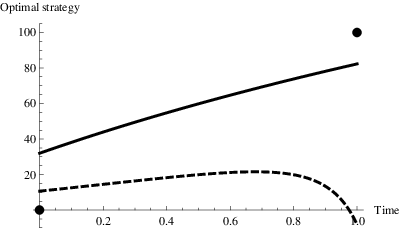
10 Conclusion
Time-varying liquidity is a fundamental property of financial markets. Its implications for optimal liquidation in limit order book markets is the focus of this paper. We find that a model with a dynamic, trading influenced spread is very robust and free of two types of price manipulation. We prove that value functions and optimal liquidation strategies in this model are of wait-region/buy-region type, which is often encountered in problems of singular control. In the literature on optimal trade execution in limit order books, the spread is often assumed to be zero. Under this assumption we show that time-varying liquidity can lead to classical as well as transaction-triggered price manipulation. For both dynamic and zero spread assumptions we derive closed form solutions for optimal strategies and provide several examples.
Appendix A Integration by parts for càglàd processes
In various proofs in this paper we need to apply stochastic analysis (e.g. integration by parts or Ito’s formula) to càglàd processes of finite variation and/or standard semimartingales. As noted in Section 2, this is always done as follows: if is a càglàd process of finite variation, we first consider the process defined by and then apply standard formulas from stochastic analysis to it. As an example of such a procedure we provide the following lemma, which is often applied in the proofs in this paper.
Lemma A.1.
(Integration by parts).
Let and be càglàd processes of finite variation and a semimartingale (in particular
càdlàg), which may have a jump at . For , we have
| (48) | |||||
| (49) |
Proof.
Let and be càdlàg processes (possibly having a jump at ) with being a semimartingale and a finite variation process. By Proposition I.4.49 a) in ?, which is a variant of integration by parts for the case where one of the semimartingales is of finite variation,
| (50) |
Equation (48) is a particular case of (50) applied to and equation (49) is a particular case of (50) applied to , where and . ∎
Appendix B Technical lemmas used in Example 9.7
Below we use the notation of Example 9.7.
Lemma B.1.
Proof.
Inequality (51) is equivalent to
The assertion now follows from our assumption on . To see this, we need to show that
which in turn is equivalent to
This is a true statement since for all and therefore
∎
Lemma B.2.
We have .
Proof.
The statement reduces to proving that . Setting we see that it is enough to establish that , which is true as, clearly, . ∎
References
- [2] [] Alfonsi, A., A. Fruth, and A. Schied, 2010, Optimal execution strategies in limit order books with general shape functions, Quantitative Finance 10, 143–157.
- [4] [] Alfonsi, A., A. Schied, and A. Slynko, 2011, Order book resilience, price manipulation, and the positive portfolio problem, Preprint.
- [6] [] Almgren, R.F., 2003, Optimal execution with nonlinear impact functions and trading-enhanced risk, Applied Mathematical Finance 10, 1–18.
- [8] [] , 2009, Optimal trading in a dynamic market, Preprint.
- [10] [] , and N. Chriss, 2001, Optimal execution of portfolio transactions, Journal of Risk 3, 5–40.
- [12] [] Bank, P., and D. Becherer, 2009, Talk: Optimal portfolio liquidation with resilient asset prices, Liquidity - Modelling Conference, Oxford.
- [14] [] Bertsimas, D., and A. Lo, 1998, Optimal control of execution costs, Journal of Financial Markets 1, 1–50.
- [16] [] Bouchaud, J. P., Y. Gefen, M. Potters, and M. Wyart, 2004, Fluctuations and response in financial markets: The subtle nature of ‘random’ price changes, Quantitative Finance 4, 176–190.
- [18] [] Chordia, Tarun, Richard Roll, and Avanidhar Subrahmanyam, 2001, Market liquidity and trading activity, Journal of Finance 56, 501–530.
- [20] [] Cont, R., S. Stoikov, and R. Talreja, 2010, A stochastic model for order book dynamics, Operations Research 58, 217–224.
- [22] [] Easley, D., and M. O’Hara, 1987, Price, trade size, and information in securities markets, Journal of Financial Economics 19, 69–90.
- [24] [] Esser, A., and B. Mönch, 2003, Modeling feedback effects with stochastic liquidity, Preprint.
- [26] [] Fruth, A., 2011, Optimal order execution with stochastic liquidity, PhD Thesis, TU Berlin.
- [28] [] Gatheral, J., 2010, No-dynamic-arbitrage and market impact, Quantitative Finance 10, 749–759.
- [30] [] , A. Schied, and A. Slynko, 2011a, Exponential resilience and decay of market impact, Econophysics of Order-driven Markets pp. 225–236.
- [32] [] , 2011b, Transient linear price impact and Fredholm integral equations, To appear in Mathematical Finance.
- [34] [] Gregory, J., and C. Lin, 1996, Constrained Optimization in the Calculus of Variations and Optimal Control Theory (Springer).
- [36] [] Huberman, G., and W. Stanzl, 2004, Price manipulation and quasi-arbitrage, Econometrica 72, 1247–1275.
- [38] [] Jacod, J., and A. Shiryaev, 2003, Limit Theorems for Stochastic Processes, 2nd edition (Springer).
- [40] [] Kempf, A., and D. Mayston, 2008, Commonalities in the liquidity of a limit order book, Journal of Financial Research 31, 25–40.
- [42] [] Kim, S.J., and S. Boyd, 2008, Optimal execution under time-inhomogeneous price impact and volatility, Preprint.
- [44] [] Kyle, A.S., 1985, Continuous auctions and insider trading, Econometrica 53, 1315–1335.
- [46] [] Large, J., 2007, Measuring the resiliency of an electronic limit order book, Journal of Financial Markets 10, 1–25.
- [48] [] Lorenz, J., and J. Osterrieder, 2009, Simulation of a limit order driven market, The Journal Of Trading 4, 23–30.
- [50] [] Madan, D. B., and W. Schoutens, 2011, Tenor specific pricing, Preprint.
- [52] [] Naujokat, F., and N. Westray, 2011, Curve following in illiquid markets, Mathematics and Financial Economics 4, 1–37.
- [54] [] Obizhaeva, A., and J. Wang, 2006, Optimal trading strategy and supply/demand dynamics, Preprint.
- [56] [] Predoiu, S., G. Shaikhet, and S.E. Shreve, 2011, Optimal execution in a general one-sided limit-order book, SIAM Journal on Financial Mathematics 2, 183–212.
- [58] [] Schöneborn, T., 2008, Trade execution in illiquid markets, PhD Thesis, TU Berlin.
- [60] [] Shiryaev, A., 1995, Probability, 2nd edition (Springer).
- [62] [] Steinmann, Georges, 2005, Order book dynamics and stochastic liquidity in risk-management, Master’s thesis ETH Zurich and University of Zurich.
- [64] [] Weiss, A., 2010, Executing large orders in a microscopic market model, Preprint.