Polar codes for classical-quantum channels

Mark M. Wilde Saikat Guha ^†^†thanks: Mark M. Wilde is with the School of Computer Science, McGill University, Montreal, Quebec H3A 2A7, Canada. Saikat Guha is with the Quantum Information Processing Group, Raytheon BBN Technologies, Cambridge, Massachusetts, USA 02138. (E-mail: mark.wilde@mcgill.ca; sguha@bbn.com)

Abstract

Holevo, Schumacher, and Westmoreland’s coding theorem guarantees the existence of codes that are capacity-achieving for the task of sending classical data over a channel with classical inputs and quantum outputs. Although they demonstrated the existence of such codes, their proof does not provide an explicit construction of codes for this task. The aim of the present paper is to fill this gap by constructing near-explicit “polar” codes that are capacity-achieving. The codes exploit the channel polarization phenomenon observed by Arikan for the case of classical channels. Channel polarization is an effect in which one can synthesize a set of channels, by “channel combining” and “channel splitting,” in which a fraction of the synthesized channels are perfect for data transmission while the other fraction are completely useless for data transmission, with the good fraction equal to the capacity of the channel. The channel polarization effect then leads to a simple scheme for data transmission: send the information bits through the perfect channels and “frozen” bits through the useless ones. The main technical contributions of the present paper are threefold. First, we leverage several known results from the quantum information literature to demonstrate that the channel polarization effect occurs for channels with classical inputs and quantum outputs. We then construct linear polar codes based on this effect, and the encoding complexity is $O(N\log N)$ , where $N$ is the blocklength of the code. We also demonstrate that a quantum successive cancellation decoder works well, in the sense that the word error rate decays exponentially with the blocklength of the code. For this last result, we exploit Sen’s recent “non-commutative union bound” that holds for a sequence of projectors applied to a quantum state.

I Introduction

Shannon’s fundamental contribution was to establish the capacity of a noisy channel as the highest rate at which a sender can reliably transmit data to a receiver [1]. His method of proof exploited the probabilistic method and was thus non-constructive. Ever since Shannon’s contribution, researchers have attempted to construct error-correcting codes that can reach the capacity of a given channel. Some of the most successful schemes for error correction are turbo codes and low-density parity-check codes [2], with numerical results demonstrating that these codes perform well for a variety of channels. In spite of the success of these codes, there is no proof that they are capacity achieving for channels other than the erasure channel [3].

Recently, Arikan constructed polar codes and proved that they are capacity achieving for a wide variety of channels [4]. Polar codes exploit the phenomenon of channel polarization, in which a simple, recursive encoding synthesizes a set of channels that polarize, in the sense that a fraction of them become perfect for transmission while the other fraction are completely noisy and thus useless for transmission. The fraction of the channels that become perfect for transmission is equal to the capacity of the channel. In addition, the complexity of both the encoding and decoding scales as $O\mathopen{}\left(N\log N\right)\mathclose{}$ , where $N$ is the blocklength of the code. Arikan developed polar codes after studying how the techniques of channel combining and channel splitting affect the rate and reliability of a channel [5]. Arikan and others have now extended the methods of polar coding to many different settings, including arbitrary discrete memoryless channels [6], source coding [7], lossy source coding [3, 8], and the multiple access channel with two senders and one receiver [9].

All of the above results are important for determining both the limits on data transmission and methods for achieving these limits on classical channels. The description of a classical channel $p_{Y|X}$ arises from modeling the signaling alphabet, the physical transmission medium, and the receiver measurement. If we are interested in accurately evaluating and reaching the true data-transmission limits of the physical channels, with an unspecified receiver measurement, and whose information carriers require a quantum-mechanical description, then it becomes necessary to invoke the laws of quantum mechanics. Examples of such channels include deep-space optical channels and ultra-low-temperature quantum-noise-limited RF channels. Achieving the classical communication capacity for such (quantum) channels often requires making collective measurements at the receiver, an action for which no classical description or implementation exists. The quantum-mechanical approach to information theory [10, 11] is not merely a formality or technicality—encoding classical information with quantum states and decoding with collective measurements on the channel outputs [12, 13] can dramatically improve data transmission rates, for example if the sender and receiver are operating in a low-power regime for a pure-loss optical channel (which is a practically relevant regime for long haul free-space terrestrial and deep-space optical communication) [14, 15]. Also, encoding with entangled inputs to the channels can increase capacity for certain channels [16], a superadditive effect which simply does not occur for classical channels.

The proof of one of the most important theorems of quantum information theory is due to Holevo [12], Schumacher, and Westmoreland [13] (HSW). They showed that the Holevo information of a quantum channel is an achievable rate for classical communication over it. Their proof of the HSW theorem bears some similarities with Shannon’s technique (including the use of random coding), but their main contribution was the construction of a quantum measurement at the receiving end that allows for reliable decoding at the Holevo information rate. Since the proof of the HSW theorem, several researchers have improved the proof’s error analysis [17], and others have demonstrated different techniques for achieving the Holevo information [18, 19, 20, 21, 22]. Very recently, Giovannetti et al. proved that a sequential decoding approach can achieve the Holevo information [23]. The sequential decoding approach has the receiver ask, through a series of dichotomic quantum measurements, whether the output of the channel was the first codeword, the second codeword, etc. (this approach is similar in spirit to a classical “jointly-typical” decoder [24]). As long as the rate of the code is less than the Holevo information, then this sequential decoder will correctly identify the transmitted codeword with asymptotically negligible error probability. Sen recently simplified the error analysis of this sequential decoding approach (rather significantly) by introducing a “non-commutative union bound” in order to bound the error probability of quantum sequential decoding [25].

In spite of the large amount of effort placed on proving that the Holevo information is achievable, there has been relatively little work on devising explicit codes that approach the Holevo information rate.¹¹ 1 This is likely due to the large amount of effort that the quantum information community has put towards quantum error correction [26], which is important for the task of transmitting quantum bits over a noisy quantum channel or for building a fault-tolerant quantum computer. Also, there might be a general belief that classical coding strategies would extend easily for sending classical information over quantum channels, but this is not the case given that collective measurements on channel outputs are required to achieve the Holevo information rate and the classical strategies do not incorporate these collective measurements. The aim of the present paper is to fill this gap by generalizing the polar coding approach to quantum channels. In doing so, we construct the first explicit class of linear codes that approach the Holevo information rate with asymptotically small error probability.

The main technical contributions of the present paper are as follows:

1.

We characterize rate with the symmetric Holevo information [27, 12, 10, 11] and reliability with the fidelity [28, 29, 10, 11] between channel outputs corresponding to different classical inputs. These parameters generalize the symmetric Shannon capacity and the Bhattacharya parameter [4], respectively, to the quantum case. We demonstrate that the symmetric Holevo information and the fidelity polarize under a recursive channel transformation similar to Arikan’s [4], by exploiting Arikan’s proof ideas [4] and several tools from the quantum information literature [30, 31, 32, 10, 33, 11].
2.

The second contribution of ours is the generalization of Arikan’s successive cancellation decoder [4] to the quantum case. We exploit ideas from quantum hypothesis testing [34, 35, 36, 37, 38] in order to construct the quantum successive cancellation decoder, and we use Sen’s recent “non-commutative union bound” [25] in order to demonstrate that the decoder performs reliably in the limit of many channel uses, while achieving the symmetric Holevo information rate.

The complexity of the encoding part of our polar coding scheme is $O\mathopen{}\left(N\log N\right)\mathclose{}$ where $N$ is the blocklength of the code (the argument for this follows directly from Arikan’s [4]). However, we have not yet been able to show that the complexity of the decoding part is $O\mathopen{}\left(N\log N\right)\mathclose{}$ (as is the case with Arikan’s decoder [4]). Determining how to simplify the complexity of the decoding part is the subject of ongoing research. For now, we should regard our contribution in this paper as a more explicit method for achieving the Holevo information rate (as compared to those from prior work [12, 13, 18, 19, 20, 21]).

One might naively think from a casual glance at our paper that Arikan’s results [4] directly apply to our quantum scenario here, but this is not the case. If one were to impose single-symbol detection on the outputs of the quantum channels,²² 2 For instance, all known conventional optical receivers are single-symbol detectors. They detect each modulated pulse individually, followed by classical postprocessing. such a procedure would induce a classical channel from input to output. In this case, Arikan’s results do apply in that they can attain the Shannon capacity of this induced classical channel.

However, the Shannon capacity of the best single-symbol detection strategy may be far below the Holevo limit [14, 15]. Attaining the Holevo information rate generally requires the receiver to perform collective measurements (physical detection of the quantum state of the entire codeword that may not be realizable by detecting single symbols one at a time). We should stress that what we are doing in this paper is different from a naive application of Arikan’s results. First, our polar coding rule depends on a quantum parameter, the fidelity, rather than the Bhattacharya distance (a classical parameter). The polar coding rule is then different from Arikan’s, and we would thus expect a larger fraction of the channels to be “good” channels than if one were to impose a single-symbol measurement and exploit Arikan’s polar coding rule with the Bhattacharya distance. Second, the quantum measurements in our quantum successive cancellation decoder are collective measurements performed on all of the channel outputs. Were it not so, then our polar coding scheme would not achieve the Holevo information rate in general.

We organize the rest of the paper as follows. The next section provides an overview of polar coding for classical-quantum channels (channels with classical inputs and quantum outputs). This overview states the main concepts and the important theorems, while saving their proofs for later in the paper. The main concepts include channel combining, channel splitting, channel polarization, rate of polarization, quantum successive cancellation decoding, and polar code performance. Section III gives more detail on how recursive channel combining and splitting lead to transformation of rate and reliability in the direction of polarization. Section IV proves that channel polarization occurs under the transformations given in Section III (the proofs in Section IV are identical to Arikan’s [4] because they merely exploit his martingale approach). We prove in Section V that the performance of the polar coding scheme is good, by analyzing the error probability under quantum successive cancellation decoding. We finally conclude in Section VI with a summary and some open questions.

II Overview of Results

Our setting involves a classical-quantum channel $W$ with a classical input $x$ and a quantum output $\rho_{x}$ :

W:x\rightarrow\rho_{x},

where $x\in\mathopen{}\left\{0,1\right\}\mathclose{}$ and $\rho_{x}$ is a unit trace, positive operator called a density operator. We can associate a probability distribution and a classical label with the states $\rho_{0}$ and $\rho_{1}$ by writing the following classical-quantum state [11]:

\rho^{XB}\equiv\frac{1}{2}\mathopen{}\left|0\right\rangle\mathclose{}\mathopen{}\left\langle 0\right|\mathclose{}^{X}\otimes\rho_{0}^{B}+\frac{1}{2}\mathopen{}\left|1\right\rangle\mathclose{}\mathopen{}\left\langle 1\right|\mathclose{}^{X}\otimes\rho_{1}^{B}.

Two important parameters for characterizing any classical-quantum channel are its rate and reliability.³³ 3 We are using the same terminology as Arikan [4]. We define the rate in terms of the channel’s symmetric Holevo information $I\mathopen{}\left(W\right)\mathclose{}$ where

I\mathopen{}\left(W\right)\mathclose{}\equiv I\mathopen{}\left(X;B\right)\mathclose{}_{\rho}.

$I\mathopen{}\left(X;B\right)\mathclose{}_{\rho}$ is the quantum mutual information of the state $\rho^{XB}$ , defined as

I\mathopen{}\left(X;B\right)\mathclose{}_{\rho}\equiv H\mathopen{}\left(X\right)\mathclose{}_{\rho}+H\mathopen{}\left(B\right)\mathclose{}_{\rho}-H\mathopen{}\left(XB\right)\mathclose{}_{\rho},

and the von Neumann entropy $H\mathopen{}\left(\sigma\right)\mathclose{}$ of any density operator $\sigma$ is defined as

H\mathopen{}\left(\sigma\right)\mathclose{}\equiv-\text{Tr}\mathopen{}\left\{\sigma\log_{2}\sigma\right\}\mathclose{}.

(Observe that the von Neumann entropy of $\sigma$ is equal to the Shannon entropy of its eigenvalues.) It is also straightforward to verify that

I\mathopen{}\left(W\right)\mathclose{}=H((\rho_{0}^{B}+\rho_{1}^{B})/2)-H(\rho_{0}^{B})/2-H(\rho_{1}^{B})/2.

The symmetric Holevo information is non-negative by concavity of von Neumann entropy, and it can never exceed one if the system $X$ is a classical binary system (as is the case for the classical-quantum state $\rho^{XB}$ ). Additionally, the symmetric Holevo information is equal to zero if there is no correlation between $X$ and $B$ . It is equal to the capacity of the channel $W$ for transmitting classical bits over it if the input prior distribution is restricted to be uniform [12, 13]. It also generalizes the symmetric capacity [4] to the quantum setting given above.

We define the reliability of the channel $W$ as the fidelity between the states $\rho_{0}$ and $\rho_{1}$ [28, 29, 10, 11]:

F\mathopen{}\left(\rho_{0},\rho_{1}\right)\mathclose{}\equiv\mathopen{}\left\|\sqrt{\rho_{0}}\sqrt{\rho_{1}}\right\|\mathclose{}_{1}^{2},

where $\mathopen{}\left\|A\right\|\mathclose{}_{1}$ is the nuclear norm of the operator $A$ :

\mathopen{}\left\|A\right\|\mathclose{}_{1}=\text{Tr}\mathopen{}\left\{\sqrt{A^{{\dagger}}A}\right\}\mathclose{}.

Let $F\mathopen{}\left(W\right)\mathclose{}$ denote the reliability of the channel $W$ :

F\mathopen{}\left(W\right)\mathclose{}\equiv F\mathopen{}\left(\rho_{0},\rho_{1}\right)\mathclose{}.

The fidelity is equal to a number between zero and one, and it characterizes how “close” two quantum states are to one another. It is equal to zero if and only if there exists a quantum measurement that can perfectly distinguish the states, and it is equal to one if the states are indistinguishable by any measurement [10, 11]. The fidelity generalizes the Bhattacharya parameter used in the classical setting [4]. Naturally, we would expect the channel $W$ to be perfectly reliable if $F\mathopen{}\left(W\right)\mathclose{}=0$ and completely unreliable if $F\mathopen{}\left(W\right)\mathclose{}=1$ . The fidelity also serves as a coarse bound on the probability of error in discriminating the states $\rho_{0}$ and $\rho_{1}$ [37, 39].

We would expect the symmetric Holevo information $I\mathopen{}\left(W\right)\mathclose{}\approx 1$ if and only if the channel’s fidelity $F\mathopen{}\left(W\right)\mathclose{}\approx 0$ and vice versa: $I\mathopen{}\left(W\right)\mathclose{}\approx 0\Leftrightarrow F\mathopen{}\left(W\right)\mathclose{}\approx 1$ . The following proposition makes this intuition rigorous, and it serves as a generalization of Arikan’s first proposition regarding the relationship between rate and reliability. We provide its proof in the appendix.

Proposition 1

For any binary input classical-quantum channel of the above form, the following bounds hold

	$\displaystyle I\mathopen{}\left(W\right)\mathclose{}$	$\displaystyle\geq\log_{2}\mathopen{}\left(\frac{2}{1+\sqrt{F\mathopen{}\left(W\right)\mathclose{}}}\right)\mathclose{},$		(1)
	$\displaystyle I\mathopen{}\left(W\right)\mathclose{}$	$\displaystyle\leq\sqrt{1-F\mathopen{}\left(W\right)\mathclose{}}.$		(2)

II-A Channel Polarization

The channel polarization phenomenon occurs after synthesizing a set of $N$ classical-quantum channels $\{W_{N}^{\mathopen{}\left(i\right)\mathclose{}}:1\leq i\leq N\}$ from $N$ independent copies of the classical-quantum channel $W$ . The effect is known as “polarization” because a fraction of the channels $W_{N}^{\mathopen{}\left(i\right)\mathclose{}}$ become perfect for data transmission,⁴⁴ 4 One cannot expect to transmit more than one classical bit over a perfect qubit channel due to Holevo’s bound [27]. in the sense that $I(W_{N}^{\mathopen{}\left(i\right)\mathclose{}})\approx 1$ for the channels in this fraction, while the channels in the complementary fraction become completely useless in the sense that $I(W_{N}^{\mathopen{}\left(i\right)\mathclose{}})\approx 0$ in the limit as $N$ becomes large. Also, the fraction of channels that do not exhibit polarization vanishes as $N$ becomes large. One can induce the polarization effect by means of channel combining and channel splitting.

II-A1 Channel Combining

Refer to caption — Fig. 1: The channel $W_{2}$ synthesized from the first level of recursion. Thick lines denote classical systems while thin lines denote quantum systems (this is our convention for the other figures as well). The depicted gate acting on the channel input is a classical controlled-NOT (CNOT) gate, where the filled-in circle acts on the source bit and the other circle acts on the target bit. Its truth table is $\mathopen{}\left(u_{1},u_{2}\right)\mathclose{}\rightarrow\mathopen{}\left(u_{1}\oplus u_{2},u_{2}\right)\mathclose{}$ .

The channel combining phase takes copies of a classical-quantum channel $W$ and builds from them an $N$ -fold classical-quantum channel $W_{N}$ in a recursive way, where $N$ is any power of two: $\ N=2^{n}$ , $n\geq 0$ . The zeroth level of recursion merely sets $W_{1}\equiv W$ . The first level of recursion combines two copies of $W_{1}$ and produces the channel $W_{2}$ , defined as

W_{2}:u_{1}u_{2}\rightarrow W_{2}^{B_{1}B_{2}}\mathopen{}\left(u_{1},u_{2}\right)\mathclose{},

(3)

where

W_{2}^{B_{1}B_{2}}\mathopen{}\left(u_{1},u_{2}\right)\mathclose{}\equiv\rho_{u_{1}\oplus u_{2}}^{B_{1}}\otimes\rho_{u_{2}}^{B_{2}}.

Figure 1 depicts this first level of recursion.

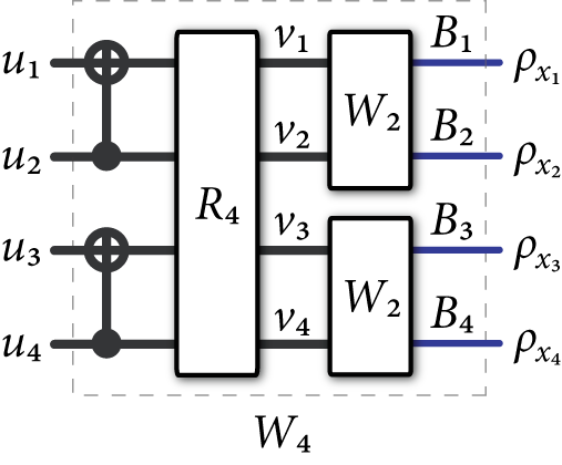
The second level of recursion takes two copies of $W_{2}$ and produces the channel $W_{4}$ :

W_{4}:u_{1}u_{2}u_{3}u_{4}\rightarrow W_{4}^{B_{1}B_{2}B_{3}B_{4}}\mathopen{}\left(u_{1},u_{2},u_{3},u_{4}\right)\mathclose{},

(4)

where

W_{4}^{B_{1}B_{2}B_{3}B_{4}}\mathopen{}\left(u_{1},u_{2},u_{3},u_{4}\right)\mathclose{}\\ \equiv W_{2}^{B_{1}B_{2}}\mathopen{}\left(u_{1}\oplus u_{2},u_{3}\oplus u_{4}\right)\mathclose{}\otimes W_{2}^{B_{3}B_{4}}\mathopen{}\left(u_{2},u_{4}\right)\mathclose{},

so that

W_{4}^{B_{1}B_{2}B_{3}B_{4}}\mathopen{}\left(u_{1},u_{2},u_{3},u_{4}\right)\mathclose{}\\ =\rho_{u_{1}\oplus u_{2}\oplus u_{3}\oplus u_{4}}^{B_{1}}\otimes\rho_{u_{3}\oplus u_{4}}^{B_{2}}\otimes\rho_{u_{2}\oplus u_{4}}^{B_{3}}\otimes\rho_{u_{4}}^{B_{4}}.

Figure 2 depicts the second level of recursion.

The operation $R_{4}$ in Figure 2 is a permutation that takes $\mathopen{}\left(u_{1},u_{2},u_{3},u_{4}\right)\mathclose{}\rightarrow\mathopen{}\left(u_{1},u_{3},u_{2},u_{4}\right)\mathclose{}$ . One can then readily check that the mapping from the row vector $u_{1}^{4}$ to the channel inputs $x_{1}^{4}$ is a linear map given by $x_{1}^{4}=u_{1}^{4}G_{4}$ with

G_{4}\equiv\begin{bmatrix}1&0&0&0\\ 1&0&1&0\\ 1&1&0&0\\ 1&1&1&1\end{bmatrix}.

The general recursion at the $n^{\text{th}}$ level is to take two copies of $W_{N/2}$ and synthesize a channel $W_{N}$ from them. The first part is to transform the input sequence $u^{N}$ according to the following rule for all $i\in\mathopen{}\left\{1,\ldots,N/2\right\}\mathclose{}$ :

	$\displaystyle s_{2i-1}$	$\displaystyle=u_{2i-1}\oplus u_{2i},$
	$\displaystyle s_{2i}$	$\displaystyle=u_{2i}.$

The next part of the transformation is a “reverse shuffle” $R_{N}$ that performs the transformation:

\mathopen{}\left(s_{1},s_{2},s_{3},s_{4},\ldots,s_{N-1},s_{N}\right)\mathclose{}\\ \rightarrow\mathopen{}\left(s_{1},s_{3},\ldots,s_{N-1},s_{2},s_{4},\ldots,s_{N}\right)\mathclose{}.

The resulting bit sequence is the input to the two copies of $W_{N/2}$ .

The overall transformation on the input sequence $u^{N}$ is a linear transformation given by $x^{N}=u^{N}G_{N}$ where

G_{N}=B_{N}F^{\otimes n},

(5)

where

F\equiv\begin{bmatrix}1&0\\ 1&1\end{bmatrix},

and $B_{N}$ is a permutation matrix known as a “bit-reversal” operation [4].

II-A2 Channel Splitting

The channel splitting phase consists of taking the channels $W_{N}$ induced by the transformation $G_{N}$ and defining new channels $W_{N}^{\mathopen{}\left(i\right)\mathclose{}}$ from them. Let $\rho_{u^{N}}$ denote the output of the channel $W_{N}$ when inputting the bit sequence $u^{N}$ . We define the $i^{\text{th}}$ split channel $W_{N}^{\mathopen{}\left(i\right)\mathclose{}}$ as follows:

W_{N}^{\mathopen{}\left(i\right)\mathclose{}}:u_{i}\rightarrow\rho_{\mathopen{}\left(i\right)\mathclose{},u_{i}}^{U_{1}^{i-1}B^{N}},

(6)

where

	$\displaystyle\rho_{\mathopen{}\left(i\right)\mathclose{},u_{i}}^{U_{1}^{i-1}B^{N}}$	$\displaystyle\equiv\sum_{u_{1}^{i-1}}\frac{1}{2^{i-1}}\mathopen{}\left\|u_{1}^{i-1}\right\rangle\mathclose{}\mathopen{}\left\langle u_{1}^{i-1}\right\|\mathclose{}^{U_{1}^{i-1}}\otimes\overline{\rho}_{u_{1}^{i}}^{B^{N}},$		(7)
	$\displaystyle\overline{\rho}_{u_{1}^{i}}^{B^{N}}$	$\displaystyle\equiv\sum_{u_{i+1}^{N}}\frac{1}{2^{N-i}}\rho_{u^{N}}^{B^{N}}.$		(8)

We can also write as an alternate notation

W_{N}^{\mathopen{}\left(i\right)\mathclose{}}(u_{i})=\rho_{\mathopen{}\left(i\right)\mathclose{},u_{i}}^{U_{1}^{i-1}B^{N}}.

These channels have the same interpretation as Arikan’s split channels [4]—they are the channels induced by a “genie-aided” quantum successive cancellation decoder, in which the $i^{\text{th}}$ decision measurement estimates $u_{i}$ given that the channel output $\rho_{u^{N}}^{B^{N}}$ is available, after observing the previous bits $u_{1}^{i-1}$ correctly, and if the distribution over $u_{i+1}^{N}$ is uniform. These split channels arise in our analysis of the error probability for quantum successive cancellation decoding.

II-A3 Channel Polarization

Our channel polarization theorem below is similar to Arikan’s Theorem 1 [4], though ours applies for classical-quantum channels with binary inputs and quantum outputs:

Theorem 2 (Channel Polarization)

The classical-quantum channels $W_{N}^{\mathopen{}\left(i\right)\mathclose{}}$ synthesized from the channel $W^{\otimes N}$ polarize, in the sense that the fraction of indices $i\in\mathopen{}\left\{1,\ldots,N\right\}\mathclose{}$ for which $I(W_{N}^{\mathopen{}\left(i\right)\mathclose{}})\in(1-\delta,1]$ goes to the symmetric Holevo information $I\mathopen{}\left(W\right)\mathclose{}$ and the fraction for which $I(W_{N}^{\mathopen{}\left(i\right)\mathclose{}})\in[0,\delta)$ goes to $1-I\mathopen{}\left(W\right)\mathclose{}$ for any $\delta\in\mathopen{}\left(0,1\right)\mathclose{}$ as $N$ goes to infinity through powers of two.

The proof of the above theorem is identical to Arikan’s proof with a martingale approach [4]. For completeness, we provide a brief proof in Section IV.

II-A4 Rate of Polarization

It is important to characterize the speed with which the polarization phenomenon comes into play for the purpose of proving this paper’s polar coding theorem. We exploit the fidelity $F(W^{\mathopen{}\left(i\right)\mathclose{}})$ of the split channels in order to characterize the rate of polarization:

F(W_{N}^{\mathopen{}\left(i\right)\mathclose{}})\equiv F(\rho_{\mathopen{}\left(i\right)\mathclose{},0}^{U_{1}^{i-1}B^{N}},\rho_{\mathopen{}\left(i\right)\mathclose{},1}^{U_{1}^{i-1}B^{N}}).

(9)

The theorem below exploits the exponential convergence results of Arikan and Telatar [40], which improved upon Arikan’s original convergence results [4] (note that we could also use the more general results in Ref. [41]):

Theorem 3 (Rate of Polarization)

Given any classical-quantum channel $W$ with $I\mathopen{}\left(W\right)\mathclose{}>0$ , any $R<I\mathopen{}\left(W\right)\mathclose{}$ , and any constant $\beta<1/2$ , there exists a sequence of sets $\mathcal{A}_{N}\subset\mathopen{}\left\{1,\ldots,N\right\}\mathclose{}$ with $\mathopen{}\left|\mathcal{A}_{N}\right|\mathclose{}\geq NR$ such that

\sum_{i\in\mathcal{A}_{N}}\sqrt{F(W_{N}^{\mathopen{}\left(i\right)\mathclose{}})}=o(2^{-N^{\beta}}).

Conversely, suppose that $R>0$ and $\beta>1/2$ . Then for any sequence of sets $\mathcal{A}_{N}\subset\mathopen{}\left\{1,\ldots,N\right\}\mathclose{}$ with $\mathopen{}\left|\mathcal{A}_{N}\right|\mathclose{}\geq NR$ , the following result holds

\max\mathopen{}\left\{\sqrt{F(W_{N}^{\mathopen{}\left(i\right)\mathclose{}})}:i\in\mathcal{A}_{N}\right\}\mathclose{}=\omega(2^{-N^{\beta}}).

The proof of this theorem exploits our results in Section III and Theorem 1 of Ref. [40].

II-B Polar Coding

The idea behind polar coding is to exploit the polarization effect for the construction of a capacity-achieving code. The sender should transmit the information bits only through the split channels $W_{N}^{\mathopen{}\left(i\right)\mathclose{}}$ for which the reliability parameter $F(W_{N}^{\mathopen{}\left(i\right)\mathclose{}})$ is close to zero. In doing so, the sender and receiver can achieve the symmetric Holevo information $I\mathopen{}\left(W\right)\mathclose{}$ of the channel $W$ .

II-B1 Coset Codes

Polar codes arise from a special class of codes that Arikan calls “ $G_{N}$ -coset codes” [4]. These $G_{N}$ -coset codes are given by the following mapping from the input sequence $u^{N}$ to the channel input sequence $x^{N}$ :

x^{N}=u^{N}G_{N},

where $G_{N}$ is the encoding matrix defined in (5). Suppose that $\mathcal{A}$ is some subset of $\mathopen{}\left\{1,\ldots,N\right\}\mathclose{}$ . Then we can write the above transformation as follows:

x^{N}=u_{\mathcal{A}}G_{N}\mathopen{}\left(\mathcal{A}\right)\mathclose{}\oplus u_{\mathcal{A}^{c}}G_{N}\mathopen{}\left(\mathcal{A}^{c}\right)\mathclose{},

(10)

where $G_{N}\mathopen{}\left(\mathcal{A}\right)\mathclose{}$ denotes the submatrix of $G_{N}$ constructed from the rows of $G_{N}$ with indices in $\mathcal{A}$ and $\oplus$ denotes vector binary addition.

Suppose that we fix the set $\mathcal{A}$ and the bit sequence $u_{\mathcal{A}^{c}}$ . The mapping in (10) then specifies a transformation from the bit sequence $u_{\mathcal{A}}$ to the channel input sequence $x^{N}$ . This mapping is equivalent to a linear encoding for a code that Arikan calls a $G_{N}$ -coset code where the sequence $u_{\mathcal{A}^{c}}G_{N}\mathopen{}\left(\mathcal{A}^{c}\right)\mathclose{}$ identifies the coset. We can fully specify a coset code by the parameter vector $\mathopen{}\left(N,K,\mathcal{A},u_{\mathcal{A}^{c}}\right)\mathclose{}$ where $N$ is the length of the code, $K=\mathopen{}\left|\mathcal{A}\right|\mathclose{}$ is the number of information bits, $\mathcal{A}$ is a set that identifies the indices for the information bits, and $u_{\mathcal{A}^{c}}$ is the vector of frozen bits. The polar coding rule specifies a way to choose the indices for the information bits based on the channel over which the sender is transmitting data.

II-B2 A Quantum Successive Cancellation Decoder

The specification of the quantum successive cancellation decoder is what mainly distinguishes Arikan’s polar codes for classical channels from ours developed here for classical-quantum channels. Let us begin with a $G_{N}$ -coset code with parameter vector $\mathopen{}\left(N,K,\mathcal{A},u_{\mathcal{A}^{c}}\right)\mathclose{}$ . The sender encodes the information bit vector $u_{\mathcal{A}}$ along with the frozen vector $u_{\mathcal{A}^{c}}$ according to the transformation in (10). The sender then transmits the encoded sequence $x^{N}$ through the classical-quantum channel, leading to a state $\rho_{x_{1}}\otimes\cdots\otimes\rho_{x_{N}}$ , which is equivalent to a state $\rho_{u^{N}}$ up to the transformation $G_{N}$ . It is then the goal of the receiver to perform a sequence of quantum measurements on the state $\rho_{u^{N}}$ in order to determine the bit sequence $u^{N}$ . We are assuming that the receiver has full knowledge of the frozen vector $u_{\mathcal{A}^{c}}$ so that he does not make mistakes when decoding these bits.

Corresponding to the split channels $W_{N}^{\mathopen{}\left(i\right)\mathclose{}}$ in (6) are the following projectors that can attempt to decide whether the input of the $i^{\text{th}}$ split channel is zero or one:

	$\displaystyle\Pi_{\mathopen{}\left(i\right)\mathclose{},0}^{U_{1}^{i-1}B^{N}}$	$\displaystyle\equiv\mathopen{}\left\{\sqrt{\rho_{\mathopen{}\left(i\right)\mathclose{},0}^{U_{1}^{i-1}B^{N}}}-\sqrt{\rho_{\mathopen{}\left(i\right)\mathclose{},1}^{U_{1}^{i-1}B^{N}}}\geq 0\right\}\mathclose{},$
	$\displaystyle\Pi_{\mathopen{}\left(i\right)\mathclose{},1}^{U_{1}^{i-1}B^{N}}$	$\displaystyle\equiv I-\Pi_{\mathopen{}\left(i\right)\mathclose{},0}^{U_{1}^{i-1}B^{N}}$
		$\displaystyle=\mathopen{}\left\{\sqrt{\rho_{\mathopen{}\left(i\right)\mathclose{},0}^{U_{1}^{i-1}B^{N}}}-\sqrt{\rho_{\mathopen{}\left(i\right)\mathclose{},1}^{U_{1}^{i-1}B^{N}}}<0\right\}\mathclose{},$

where $\sqrt{A}$ denotes the square root of a positive operator $A$ , $\mathopen{}\left\{B\geq 0\right\}\mathclose{}$ denotes the projector onto the positive eigenspace of a Hermitian operator $B$ , and $\mathopen{}\left\{B<0\right\}\mathclose{}$ denotes the projection onto the negative eigenspace of $B$ . After some calculations, we can readily see that

	$\displaystyle\Pi_{\mathopen{}\left(i\right)\mathclose{},0}^{U_{1}^{i-1}B^{N}}$	$\displaystyle=\sum_{u_{1}^{i-1}}\mathopen{}\left\|u_{1}^{i-1}\right\rangle\mathclose{}\mathopen{}\left\langle u_{1}^{i-1}\right\|\mathclose{}^{U_{1}^{i-1}}\otimes\Pi_{\mathopen{}\left(i\right)\mathclose{},u_{1}^{i-1}0}^{B^{N}},$		(11)
	$\displaystyle\Pi_{\mathopen{}\left(i\right)\mathclose{},1}^{U_{1}^{i-1}B^{N}}$	$\displaystyle=\sum_{u_{1}^{i-1}}\mathopen{}\left\|u_{1}^{i-1}\right\rangle\mathclose{}\mathopen{}\left\langle u_{1}^{i-1}\right\|\mathclose{}^{U_{1}^{i-1}}\otimes\Pi_{\mathopen{}\left(i\right)\mathclose{},u_{1}^{i-1}1}^{B^{N}},$		(12)

where

	$\displaystyle\Pi_{\mathopen{}\left(i\right)\mathclose{},u_{1}^{i-1}0}^{B^{N}}$	$\displaystyle\equiv\mathopen{}\left\{\sqrt{\overline{\rho}_{u_{1}^{i-1}0}^{B^{N}}}-\sqrt{\overline{\rho}_{u_{1}^{i-1}1}^{B^{N}}}\geq 0\right\}\mathclose{},$
	$\displaystyle\Pi_{\mathopen{}\left(i\right)\mathclose{},u_{1}^{i-1}1}^{B^{N}}$	$\displaystyle\equiv\mathopen{}\left\{\sqrt{\overline{\rho}_{u_{1}^{i-1}0}^{B^{N}}}-\sqrt{\overline{\rho}_{u_{1}^{i-1}1}^{B^{N}}}<0\right\}\mathclose{}.$

The above observations lead to a method for a successive cancellation decoder similar to Arikan’s [4], with the following decoding rule:

\hat{u}_{i}=\mathopen{}\left\{\begin{array}[c]{cc}u_{i}&\text{if }i\in\mathcal{A}^{c}\\ h\mathopen{}\left(\hat{u}_{1}^{i-1}\right)\mathclose{}&\text{if }i\in\mathcal{A}\end{array}\right.\mathclose{},

where $h\mathopen{}\left(\hat{u}_{1}^{i-1}\right)\mathclose{}$ is the outcome of the following $i^{\text{th}}$ measurement on the output of the channel (after $i-1$ measurements have already been performed):

\mathopen{}\left\{\Pi_{\mathopen{}\left(i\right)\mathclose{},\hat{u}_{1}^{i-1}0}^{B^{N}},\Pi_{\mathopen{}\left(i\right)\mathclose{},\hat{u}_{1}^{i-1}1}^{B^{N}}\right\}\mathclose{}.

We are assuming that the measurement device outputs “0” if the outcome $\Pi_{\mathopen{}\left(i\right)\mathclose{},\hat{u}_{1}^{i-1}0}^{B^{N}}$ occurs and it outputs “1” otherwise. (Note that we can set $\Pi_{\mathopen{}\left(i\right)\mathclose{},\hat{u}_{1}^{i-1}u_{i}}^{B^{N}}=I$ if the bit $u_{i}$ is a frozen bit.) The above sequence of measurements for the whole bit stream $u^{N}$ corresponds to a positive operator-valued measure (POVM) $\mathopen{}\left\{\Lambda_{u^{N}}\right\}\mathclose{}$ where

\Lambda_{u^{N}}\equiv\Pi_{\mathopen{}\left(1\right)\mathclose{},u_{1}}^{B^{N}}\cdots\Pi_{\mathopen{}\left(i\right)\mathclose{},u_{1}^{i-1}u_{i}}^{B^{N}}\cdots\\ \cdots\Pi_{\mathopen{}\left(N\right)\mathclose{},u_{1}^{N-1}u_{N}}^{B^{N}}\cdots\Pi_{\mathopen{}\left(i\right)\mathclose{},u_{1}^{i-1}u_{i}}^{B^{N}}\cdots\Pi_{\mathopen{}\left(1\right)\mathclose{},u_{1}}^{B^{N}},

\sum_{u_{\mathcal{A}}}\Lambda_{u^{N}}=I^{B^{N}}.

The above decoding strategy is suboptimal in two regards. First, the decoder assumes that the future bits are unknown (and random) even if the receiver has full knowledge of the future frozen bits (this suboptimality is similar to the suboptimality of Arikan’s decoder [4]). Second, the measurement operators for making a decision are suboptimal as well because we choose them to be projectors onto the positive eigenspace of the difference of the square roots of two density operators. The optimal bitwise decision rule is to choose these operators to be the Helstrom-Holevo projector onto the positive eigenspace of the difference of two density operators [34, 35]. Having our quantum successive cancellation decoder operate in these two different suboptimal ways allows for us to analyze its performance easily (though, note that we could just as well have used Helstrom-Holevo measurements to obtain bounds on the error probability). This suboptimality is asymptotically negligible because the symmetric Holevo information is still an achievable rate for data transmission even for the above choice of measurement operators.

II-B3 Polar Code Performance

The probability of error $P_{e}\mathopen{}\left(N,K,\mathcal{A},u_{\mathcal{A}^{c}}\right)\mathclose{}$ for code length $N$ , number $K$ of information bits, set $\mathcal{A}$ of information bits, and choice $u_{\mathcal{A}^{c}}$ for the frozen bits is as follows:

		$\displaystyle P_{e}\mathopen{}\left(N,K,\mathcal{A},u_{\mathcal{A}^{c}}\right)\mathclose{}$
		$\displaystyle=\frac{1}{2^{K}}\sum_{u_{\mathcal{A}}}\text{Tr}\mathopen{}\left\{\mathopen{}\left(I-\Lambda_{u^{N}}\right)\mathclose{}\rho_{u^{N}}\right\}\mathclose{}$
		$\displaystyle=1-\frac{1}{2^{K}}\sum_{u_{\mathcal{A}}}\text{Tr}\mathopen{}\left\{\Lambda_{u^{N}}\rho_{u^{N}}\right\}\mathclose{}$
		$\displaystyle=1-\frac{1}{2^{K}}\sum_{u_{\mathcal{A}}}\text{Tr}\bigg\{\Pi_{\mathopen{}\left(N\right)\mathclose{},u_{1}^{N-1}u_{N}}^{B^{N}}\cdots\Pi_{\mathopen{}\left(i\right)\mathclose{},u_{1}^{i-1}u_{i}}^{B^{N}}\cdots$
		$\displaystyle\ \ \ \cdots\Pi_{\mathopen{}\left(1\right)\mathclose{},u_{1}}^{B^{N}}\ \rho_{u^{N}}\ \Pi_{\mathopen{}\left(1\right)\mathclose{},u_{1}}^{B^{N}}\cdots\Pi_{\mathopen{}\left(i\right)\mathclose{},u_{1}^{i-1}u_{i}}^{B^{N}}\cdots\Pi_{\mathopen{}\left(N\right)\mathclose{},u_{1}^{N-1}u_{N}}^{B^{N}}\bigg\},$

where we are assuming a particular choice of the bits $u_{\mathcal{A}^{c}}$ in the sequence of projectors $\Pi_{\mathopen{}\left(N\right)\mathclose{},u_{1}^{N-1}u_{N}}^{B^{N}}$ $\cdots$ $\Pi_{\mathopen{}\left(i\right)\mathclose{},u_{1}^{i-1}u_{i}}^{B^{N}}$ $\cdots$ $\Pi_{\mathopen{}\left(1\right)\mathclose{},u_{1}}^{B^{N}}$ and the convention mentioned before that $\Pi_{\mathopen{}\left(i\right)\mathclose{},u_{1}^{i-1}u_{i}}^{B^{N}}=I$ if $u_{i}$ is a frozen bit. We are also assuming that the sender transmits the information sequence $u_{\mathcal{A}}$ with uniform probability $2^{-K}$ . The probability of error $P_{e}\mathopen{}\left(N,K,\mathcal{A}\right)\mathclose{}$ averaged over all choices of the frozen bits is then

		$\displaystyle P_{e}\mathopen{}\left(N,K,\mathcal{A}\right)\mathclose{}$
		$\displaystyle=\frac{1}{2^{N-K}}\sum_{u_{\mathcal{A}^{c}}}P_{e}\mathopen{}\left(N,K,\mathcal{A},u_{\mathcal{A}^{c}}\right)\mathclose{}$
		$\displaystyle=1-\frac{1}{2^{N}}\sum_{u^{N}}\text{Tr}\bigg\{\Pi_{\mathopen{}\left(N\right)\mathclose{},u_{1}^{N-1}u_{N}}^{B^{N}}\cdots\Pi_{\mathopen{}\left(i\right)\mathclose{},u_{1}^{i-1}u_{i}}^{B^{N}}\cdots$
		$\displaystyle\ \ \ \ \cdots\Pi_{\mathopen{}\left(1\right)\mathclose{},u_{1}}^{B^{N}}\ \rho_{u^{N}}\ \Pi_{\mathopen{}\left(1\right)\mathclose{},u_{1}}^{B^{N}}\cdots\Pi_{\mathopen{}\left(i\right)\mathclose{},u_{1}^{i-1}u_{i}}^{B^{N}}\cdots\Pi_{\mathopen{}\left(N\right)\mathclose{},u_{1}^{N-1}u_{N}}^{B^{N}}\bigg\}.$		(13)

One of the main contributions of this paper is the following proposition regarding the average ensemble performance of polar codes with a quantum successive cancellation decoder:

Proposition 4

For any classical-quantum channel $W$ with binary inputs and quantum outputs and any choice of $\mathopen{}\left(N,K,\mathcal{A}\right)\mathclose{}$ , the following bound holds

P_{e}\mathopen{}\left(N,K,\mathcal{A}\right)\mathclose{}\leq 2\sqrt{\sum_{i\in\mathcal{A}}\frac{1}{2}\sqrt{F(W_{N}^{\mathopen{}\left(i\right)\mathclose{}})}}.

Thus, there exists a frozen vector $u_{\mathcal{A}^{c}}$ for each $\mathopen{}\left(N,K,\mathcal{A}\right)\mathclose{}$ such that

P_{e}\mathopen{}\left(N,K,\mathcal{A},u_{\mathcal{A}^{c}}\right)\mathclose{}\leq 2\sqrt{\sum_{i\in\mathcal{A}}\frac{1}{2}\sqrt{F(W_{N}^{\mathopen{}\left(i\right)\mathclose{}})}}.

II-B4 Polar Coding Theorem

Proposition 4 immediately leads to the definition of polar codes for classical-quantum channels:

Definition 5 (Polar Code)

A polar code for $W$ is a $G_{N}$ -coset code with parameters $\mathopen{}\left(N,K,\mathcal{A},u_{\mathcal{A}^{c}}\right)\mathclose{}$ where the information set $\mathcal{A}$ is such that $\mathopen{}\left|\mathcal{A}\right|\mathclose{}=K$ and

F(W_{N}^{\mathopen{}\left(i\right)\mathclose{}})\leq F(W_{N}^{\mathopen{}\left(j\right)\mathclose{}})\text{ for all }i\in\mathcal{A}\text{ and }j\in\mathcal{A}^{c}.

We can finally state the polar coding theorem for classical-quantum channels. Consider a classical-quantum channel $W$ and a real number $R\geq 0$ . Let

P_{e}\mathopen{}\left(N,R\right)\mathclose{}=P_{e}\mathopen{}\left(N,\mathopen{}\left\lfloor NR\right\rfloor\mathclose{},\mathcal{A}\right)\mathclose{},

with the information bit set chosen according to the polar coding rule in Definition 5. So $P_{e}\mathopen{}\left(N,\mathcal{A}\right)\mathclose{}$ is the block error probability for polar coding over $W$ with blocklength $N$ , rate $R$ , and quantum successive cancellation decoding averaged uniformly over the frozen bits $u_{\mathcal{A}^{c}}$ .

Theorem 6 (Polar Coding Theorem)

For any classical-quantum channel $W$ with binary inputs and quantum outputs, a fixed $R<I\mathopen{}\left(W\right)\mathclose{}$ , and $\beta<1/2$ , the block error probability $P_{e}\mathopen{}\left(N,R\right)\mathclose{}$ satisfies the following bound:

P_{e}\mathopen{}\left(N,R\right)\mathclose{}=o(2^{-\frac{1}{2}N^{\beta}}).

The polar coding theorem above follows as a straightforward corollary of Theorem 3 and Proposition 4.

III Recursive Channel Transformations

This section delves into more detail regarding recursive channel combining and channel splitting. Recall the channel combining in (3-5) and the channel splitting in (6). These allowed for us to take $N$ independent copies of a classical-quantum channel $W^{\otimes N}$ and transform them into the $N$ split channels $W_{N}^{\mathopen{}\left(1\right)\mathclose{}}$ , …, $W_{N}^{\mathopen{}\left(N\right)\mathclose{}}$ . We show here how to break the channel transformation into a series of single-step transformations. Much of the discussion here parallels Arikan’s discussion in Sections II and III of Ref. [4].

We obtain a pair of channels $W^{-}$ and $W^{+}$ from two independent copies of a channel $W:x\rightarrow\rho_{x}$ by a single-step transformation if it holds that

W^{-}:u_{1}\rightarrow\rho_{u_{1}}^{-},

where

\rho_{u_{1}}^{-}\equiv\sum_{u_{2}}\frac{1}{2}\rho_{u_{2}\oplus u_{1}}^{B_{1}}\otimes\rho_{u_{2}}^{B_{2}}.

(14)

Also, it should hold that

W^{+}:u_{2}\rightarrow\rho_{u_{2}}^{+},

where

	$\displaystyle\rho_{u_{2}}^{+}$	$\displaystyle\equiv\sum_{u_{1}}\frac{1}{2}\mathopen{}\left\|u_{1}\right\rangle\mathclose{}\mathopen{}\left\langle u_{1}\right\|\mathclose{}^{U_{1}}\otimes\rho_{u_{2}\oplus u_{1}}^{B_{1}}\otimes\rho_{u_{2}}^{B_{2}}$		(15)
		$\displaystyle=\mathopen{}\left(\sum_{u_{1}}\frac{1}{2}\mathopen{}\left\|u_{1}\right\rangle\mathclose{}\mathopen{}\left\langle u_{1}\right\|\mathclose{}^{U_{1}}\otimes\rho_{u_{2}\oplus u_{1}}^{B_{1}}\right)\mathclose{}\otimes\rho_{u_{2}}^{B_{2}}.$

We use the following notation to denote such a transformation:

\mathopen{}\left(W,W\right)\mathclose{}\rightarrow\mathopen{}\left(W^{-},W^{+}\right)\mathclose{}.

Additionally, we choose the notation $W^{-}$ and $W^{+}$ so that $W^{-}$ denotes the worse channel and $W^{+}$ denotes the better channel. Figure 3 depicts the channels $W^{-}$ and $W^{+}$ .

Thus, from the above, we can write $\mathopen{}\left(W,W\right)\mathclose{}\rightarrow(W_{2}^{\mathopen{}\left(1\right)\mathclose{}},W_{2}^{\mathopen{}\left(2\right)\mathclose{}})$ because, by the definition in (6), we have

	$\displaystyle W_{2}^{\mathopen{}\left(1\right)\mathclose{}}\mathopen{}\left(u_{1}\right)\mathclose{}$	$\displaystyle=\sum_{u_{2}}\frac{1}{2}\rho_{u_{1}\oplus u_{2}}^{B_{1}}\otimes\rho_{u_{2}}^{B_{2}},$
	$\displaystyle W_{2}^{\mathopen{}\left(2\right)\mathclose{}}\mathopen{}\left(u_{2}\right)\mathclose{}$	$\displaystyle=\sum_{u_{1}}\frac{1}{2}\mathopen{}\left\|u_{1}\right\rangle\mathclose{}\mathopen{}\left\langle u_{1}\right\|\mathclose{}^{U_{1}}\otimes\rho_{u_{1}\oplus u_{2}}^{B_{1}}\otimes\rho_{u_{2}}^{B_{2}}.$

We can actually write more generally

(W_{N}^{\mathopen{}\left(i\right)\mathclose{}},W_{N}^{\mathopen{}\left(i\right)\mathclose{}})\rightarrow(W_{2N}^{\mathopen{}\left(2i-1\right)\mathclose{}},W_{2N}^{\mathopen{}\left(2i\right)\mathclose{}}),

(16)

which follows as a corollary to

Proposition 7

For any $n\geq 0$ , $N=2^{n}$ , and $1\leq i\leq N$ , it holds that

	$\displaystyle W_{2N}^{\mathopen{}\left(2i-1\right)\mathclose{}}\mathopen{}\left(u_{2i-1}\right)\mathclose{}$	$\displaystyle=\sum_{u_{2i}}\frac{1}{2}W_{N}^{\mathopen{}\left(i\right)\mathclose{}}\mathopen{}\left(u_{2i-1}\oplus u_{2i}\right)\mathclose{}\otimes W_{N}^{\mathopen{}\left(i\right)\mathclose{}}\mathopen{}\left(u_{2i}\right)\mathclose{},$		(17)
	$\displaystyle W_{2N}^{\mathopen{}\left(2i\right)\mathclose{}}\mathopen{}\left(u_{2i}\right)\mathclose{}$	$\displaystyle=W_{N}^{\mathopen{}\left(i\right)\mathclose{}}\mathopen{}\left(u_{2i-1}\oplus u_{2i}\right)\mathclose{}\otimes W_{N}^{\mathopen{}\left(i\right)\mathclose{}}\mathopen{}\left(u_{2i}\right)\mathclose{},$		(18)

with $W_{N}^{\mathopen{}\left(i\right)\mathclose{}}$ defined in (6).

Proof:

The proof of the above proposition is similar to the proof of Arikan’s Proposition 3 [4]. ∎

We can justify the relationship in (16) by observing that (17) and (18) have the same form as (14) and (15) with the following substitutions:

	$\displaystyle W$	$\displaystyle\leftarrow W_{N}^{\mathopen{}\left(i\right)\mathclose{}},$
	$\displaystyle W^{+}$	$\displaystyle\leftarrow W_{2N}^{\mathopen{}\left(2i\right)\mathclose{}},$
	$\displaystyle W^{-}$	$\displaystyle\leftarrow W_{2N}^{\mathopen{}\left(2i-1\right)\mathclose{}},$
	$\displaystyle u_{1}$	$\displaystyle\leftarrow u_{2i-1},$
	$\displaystyle u_{2}$	$\displaystyle\leftarrow u_{2i}.$

III-A Transformation of Rate and Reliability

This section considers how both the rate $I(W_{N}^{(i)})$ and reliability $F(W_{N}^{(i)})$ evolve under the general transformation in (16). All proofs of the results in this section appear in the appendix.

Proposition 8

Suppose that $(W,W)\rightarrow(W^{-},W^{+})$ for some channels satisfying (14-15). Then the following rate conservation and polarizing relations hold

	$\displaystyle I\mathopen{}\left(W^{-}\right)\mathclose{}+I\mathopen{}\left(W^{+}\right)\mathclose{}$	$\displaystyle=2I\mathopen{}\left(W\right)\mathclose{},$		(19)
	$\displaystyle I\mathopen{}\left(W^{-}\right)\mathclose{}$	$\displaystyle\leq I\mathopen{}\left(W^{+}\right)\mathclose{}.$		(20)

We can conclude from the above two relations that

I\mathopen{}\left(W^{-}\right)\mathclose{}\leq I\mathopen{}\left(W\right)\mathclose{}\leq I\mathopen{}\left(W^{+}\right)\mathclose{}.

The following proposition states how the reliability evolves under the channel transformation:

Proposition 9

Suppose $\mathopen{}\left(W,W\right)\mathclose{}\rightarrow\mathopen{}\left(W^{-},W^{+}\right)\mathclose{}$ for some channels satisfying (14-15). Then

$\displaystyle\sqrt{F\mathopen{}\left(W^{+}\right)\mathclose{}}$	$\displaystyle=F\mathopen{}\left(W\right)\mathclose{},$	(21)
$\displaystyle\sqrt{F\mathopen{}\left(W^{-}\right)\mathclose{}}$	$\displaystyle\leq 2\sqrt{F\mathopen{}\left(W\right)\mathclose{}}-F\mathopen{}\left(W\right)\mathclose{},$	(22)
$\displaystyle F\mathopen{}\left(W^{-}\right)\mathclose{}$	$\displaystyle\geq F\mathopen{}\left(W\right)\mathclose{}\geq F\mathopen{}\left(W^{+}\right)\mathclose{}.$	(23)

By combining (21) with (22), we observe that the reliability only improves under a single-step transformation:

\sqrt{F\mathopen{}\left(W^{-}\right)\mathclose{}}+\sqrt{F\mathopen{}\left(W^{+}\right)\mathclose{}}\leq 2\sqrt{F\mathopen{}\left(W\right)\mathclose{}}.

The above propositions for the single-step transformation lead us to the following proposition in the general case:

Proposition 10

For any classical-quantum channel $W$ , $N=2^{n}$ , $n\geq 0$ , and $1\leq i\leq N$ , the local transformation in (16) preserves rate and improves reliability in the following sense:

	$\displaystyle I(W_{2N}^{\mathopen{}\left(2i-1\right)\mathclose{}})+I(W_{2N}^{\mathopen{}\left(2i\right)\mathclose{}})$	$\displaystyle=2I(W_{N}^{\mathopen{}\left(i\right)\mathclose{}}),$		(24)
	$\displaystyle\sqrt{F(W_{2N}^{\mathopen{}\left(2i-1\right)\mathclose{}})}+\sqrt{F(W_{2N}^{\mathopen{}\left(2i\right)\mathclose{}})}$	$\displaystyle\leq 2\sqrt{F(W_{N}^{\mathopen{}\left(i\right)\mathclose{}})}.$		(25)

Channel splitting moves rate and reliability “away from the center”:

	$\displaystyle I(W_{2N}^{\mathopen{}\left(2i-1\right)\mathclose{}})$	$\displaystyle\leq I(W_{N}^{\mathopen{}\left(i\right)\mathclose{}})\leq I(W_{2N}^{\mathopen{}\left(2i\right)\mathclose{}}),$
	$\displaystyle\sqrt{F(W_{2N}^{\mathopen{}\left(2i-1\right)\mathclose{}})}$	$\displaystyle\geq\sqrt{F(W_{N}^{\mathopen{}\left(i\right)\mathclose{}})}\geq\sqrt{F(W_{2N}^{\mathopen{}\left(2i\right)\mathclose{}})}.$

The reliability terms satisfy

	$\displaystyle\sqrt{F(W_{2N}^{\mathopen{}\left(2i\right)\mathclose{}})}$	$\displaystyle=F(W_{N}^{\mathopen{}\left(i\right)\mathclose{}}),$		(26)
	$\displaystyle\sqrt{F(W_{2N}^{\mathopen{}\left(2i-1\right)\mathclose{}})}$	$\displaystyle\leq 2\sqrt{F(W_{N}^{\mathopen{}\left(i\right)\mathclose{}})}-F(W_{N}^{\mathopen{}\left(i\right)\mathclose{}}),$		(27)

and the cumulative rate and reliability satisfy

	$\displaystyle\sum_{i=1}^{N}I(W_{N}^{\mathopen{}\left(i\right)\mathclose{}})$	$\displaystyle=N\ I\mathopen{}\left(W\right)\mathclose{},$		(28)
	$\displaystyle\sum_{i=1}^{N}\sqrt{F(W_{N}^{\mathopen{}\left(i\right)\mathclose{}})}$	$\displaystyle\leq N\ \sqrt{F\mathopen{}\left(W\right)\mathclose{}}.$		(29)

The above proposition follows directly from Propositions 7, 8, and 9. The relations in (28) and (29) follow from applying (24) and (25) repeatedly.

IV Channel Polarization

We are now in a position to prove Theorem 2 on channel polarization. The idea behind the proof of this theorem is identical to Arikan’s proof of his Theorem 1 in Ref. [4]—with the relationships in Propositions 8 and 9 already established, we can readily exploit the martingale proof technique. Thus, we only provide a brief summary of the proof of Theorem 2 by following the presentation in Chapter 2 of Ref. [3].

Consider the channel $W_{N}^{\mathopen{}\left(i\right)\mathclose{}}$ . Let $b_{1}\cdots b_{n}$ denote an $n$ -bit binary expansion of the channel index $i$ and let $W_{\mathopen{}\left(b_{1}\cdots b_{n}\right)\mathclose{}}=W_{N}^{\mathopen{}\left(i\right)\mathclose{}}$ . Then we can construct the channel $W_{\mathopen{}\left(b_{1}\cdots b_{k}\right)\mathclose{}}$ by combining two copies of $W_{\mathopen{}\left(b_{1}\cdots b_{k-1}\right)\mathclose{}}$ according to (17) if $b_{k}=0$ or by combining two copies of $W_{\mathopen{}\left(b_{1}\cdots b_{k-1}\right)\mathclose{}}$ according to (18) if $b_{k}=1$ . We repeatedly construct all the way from $b_{1}$ until $b_{n}$ with the above rule.

Arikan’s idea was to represent the channel construction as a random birth process in order to analyze its limiting behavior. In order to do so, we let $\mathopen{}\left\{B_{n}:n\geq 1\right\}\mathclose{}$ be a sequence of IID uniform Bernoulli random variables, where we define each over a probability space $(\Omega,\mathcal{F},P)$ . Let $\mathcal{F}_{0}$ denote the trivial $\sigma$ -field. Also, let $\mathopen{}\left\{\mathcal{F}_{n}:n\geq 1\right\}\mathclose{}$ denote the $\sigma$ -fields that the random variables $\mathopen{}\left(B_{1},\ldots,B_{n}\right)\mathclose{}$ generate. We also assume that $\mathcal{F}_{0}\subseteq\mathcal{F}_{1}\subseteq\mathcal{\cdots}\subseteq\mathcal{F}_{n}$ . Let $W_{0}=W$ and let $\mathopen{}\left\{W_{n}:n\geq 0\right\}\mathclose{}$ denote a sequence of operator-valued random variables that forms a tree process where $W_{n+1}$ is constructed from two copies of $W_{n}$ according to (17) if $B_{n}=0$ and according to (18) if $B_{n}=1$ . The output space of the operator-valued random variable $W_{n}$ is equal to $\{W_{2^{n}}^{\mathopen{}\left(i\right)\mathclose{}}\}_{i=1}^{2^{n}}$ . We are not really concerned with the channel process $\mathopen{}\left\{W_{n}:n\geq 0\right\}\mathclose{}$ but more so with the fidelities $\{F(W_{N}^{\mathopen{}\left(i\right)\mathclose{}})\}$ and Holevo informations $\{I(W_{N}^{\mathopen{}\left(i\right)\mathclose{}})\}$ . Thus, we can simply analyze the limiting behavior of the two random processes $\{F_{n}:n\geq 0\}\equiv\{\sqrt{F(W_{n})}:n\geq 0\}$ and $\{I_{n}:n\geq 0\}\equiv\{I(W_{n}):n\geq 0\}$ . By the definitions of the random variables $F_{n}$ and $I_{n}$ , it follows that

	$\displaystyle\Pr\mathopen{}\left\{I_{n}\in\mathopen{}\left(a,b\right)\mathclose{}\right\}\mathclose{}$	$\displaystyle=\frac{1}{2^{n}}\|\{i:I(W_{2^{n}}^{\mathopen{}\left(i\right)\mathclose{}})\in\mathopen{}\left(a,b\right)\mathclose{}\}\|,$
	$\displaystyle\Pr\mathopen{}\left\{F_{n}\in\mathopen{}\left(a,b\right)\mathclose{}\right\}\mathclose{}$	$\displaystyle=\frac{1}{2^{n}}\|\{i:F(W_{2^{n}}^{\mathopen{}\left(i\right)\mathclose{}})\in\mathopen{}\left(a,b\right)\mathclose{}\}\|.$

We then have the following lemma.

Lemma 11

The sequence $\{\mathopen{}\left(F_{n},\mathcal{F}_{n}\right)\mathclose{}:n\geq 0\}$ is a bounded super-martingale, and the sequence $\{\mathopen{}\left(I_{n},\mathcal{F}_{n}\right)\mathclose{}:n\geq 0\}$ is a bounded martingale.

Proof:

Let $b_{1}\cdots b_{n}$ be a particular realization of the random sequence $B_{1}\cdots B_{n}$ . Then the conditional expectation satisfies

		$\displaystyle\mathbb{E}\mathopen{}\left\{I_{n+1}\ \|\ B_{1}=b_{1},\ldots,B_{n}=b_{n}\right\}\mathclose{}$
		$\displaystyle=\frac{1}{2}I\mathopen{}\left(W_{\mathopen{}\left(b_{1},\ldots,b_{n},0\right)\mathclose{}}\right)\mathclose{}+\frac{1}{2}I\mathopen{}\left(W_{\mathopen{}\left(b_{1},\ldots,b_{n},1\right)\mathclose{}}\right)\mathclose{}$
		$\displaystyle=I\mathopen{}\left(W_{\mathopen{}\left(b_{1},\ldots,b_{n}\right)\mathclose{}}\right)\mathclose{}$
		$\displaystyle=I_{n},$

where the second equality follows from the definition of $W_{\mathopen{}\left(b_{1},\ldots,b_{n},0\right)\mathclose{}}$ and $W_{\mathopen{}\left(b_{1},\ldots,b_{n},1\right)\mathclose{}}$ and Proposition 10. The proof for $\mathopen{}\left\{F_{n}\right\}\mathclose{}$ similarly follows from the definitions and Proposition 10. The boundedness condition follows because $0\leq I\mathopen{}\left(W\right)\mathclose{},F\mathopen{}\left(W\right)\mathclose{}\leq 1$ for any classical-quantum channel $W$ with binary inputs and quantum outputs. ∎

We can now finally prove Theorem 2 regarding channel polarization. Given that $\mathopen{}\left\{I_{n}\right\}\mathclose{}$ is a bounded martingale and $\mathopen{}\left\{F_{n}\right\}\mathclose{}$ is a bounded super-martingale, the limits $\lim_{n\rightarrow\infty}I_{n}$ and $\lim_{n\rightarrow\infty}F_{n}$ converge almost surely and in $\mathcal{L}_{1}$ to the random variables $I_{\infty}$ and $F_{\infty}$ . The convergence implies that $\mathbb{E}\mathopen{}\left\{\mathopen{}\left|F_{n+1}-F_{n}\right|\mathclose{}\right\}\mathclose{}\rightarrow 0$ as $n\rightarrow\infty$ . By the definition of the process $\mathopen{}\left\{F_{n}\right\}\mathclose{}$ , it holds that $F_{n+1}=F_{n}^{2}$ with probability $\frac{1}{2}$ , so that

\mathbb{E}\mathopen{}\left\{\mathopen{}\left|F_{n+1}-F_{n}\right|\mathclose{}\right\}\mathclose{}\geq\frac{1}{2}\mathbb{E}\mathopen{}\left\{\mathopen{}\left|F_{n}\mathopen{}\left(1-F_{n}\right)\mathclose{}\right|\mathclose{}\right\}\mathclose{}\geq 0.

It then follows that $\mathbb{E}\mathopen{}\left\{\mathopen{}\left|F_{n}\mathopen{}\left(1-F_{n}\right)\mathclose{}\right|\mathclose{}\right\}\mathclose{}\rightarrow 0$ as $n\rightarrow\infty$ , which in turn implies that $\mathbb{E}\mathopen{}\left\{\mathopen{}\left|F_{\infty}\mathopen{}\left(1-F_{\infty}\right)\mathclose{}\right|\mathclose{}\right\}\mathclose{}=0$ . We conclude that $F_{\infty}\in\mathopen{}\left\{0,1\right\}\mathclose{}$ almost surely. Combining this result with Proposition 1 proves that $I_{\infty}\in\mathopen{}\left\{0,1\right\}\mathclose{}$ almost surely. Finally, we have that $\Pr\mathopen{}\left\{I_{\infty}=1\right\}\mathclose{}=\mathbb{E}\mathopen{}\left\{I_{\infty}\right\}\mathclose{}=\mathbb{E}\mathopen{}\left\{I_{0}\right\}\mathclose{}=I\mathopen{}\left(W\right)\mathclose{}$ because $I_{n}$ is a martingale.

V Performance of Polar Coding

We can now analyze the performance under the above successive cancellation decoding scheme and provide a proof of Proposition 4. The proof of Theorem 6 readily follows by applying Proposition 4 and Theorem 3.

First recall the following “non-commutative union bound” of Sen (Lemma 3 in Ref. [25]):

1-\text{Tr}\mathopen{}\left\{\Pi_{N}\cdots\Pi_{1}\rho\Pi_{1}\cdots\Pi_{N}\right\}\mathclose{}\leq 2\sqrt{\sum_{i=1}^{N}\text{Tr}\mathopen{}\left\{\mathopen{}\left(I-\Pi_{i}\right)\mathclose{}\rho\right\}\mathclose{}},

(30)

which holds for projectors $\Pi_{1}$ , …, $\Pi_{N}$ and a density operator $\rho$ .⁵⁵ 5 We say that Sen’s bound is a “non-commutative union bound” because it is analogous to the following union bound from probability theory: $\Pr\mathopen{}\left\{\mathopen{}\left(A_{1}\cap\cdots\cap A_{N}\right)\mathclose{}^{c}\right\}\mathclose{}=\Pr\mathopen{}\left\{A_{1}^{c}\cup\cdots\cup A_{N}^{c}\right\}\mathclose{}\leq\sum_{i=1}^{N}\Pr\mathopen{}\left\{A_{i}^{c}\right\}\mathclose{}$ , where $A_{1}$ , …, $A_{N}$ are events. The analogous bound for projector logic would be Tr $\mathopen{}\left\{\mathopen{}\left(I-\Pi_{1}\cdots\Pi_{N}\cdots\Pi_{1}\right)\mathclose{}\rho\right\}\mathclose{}\leq\sum_{i=1}^{N}$ Tr $\mathopen{}\left\{\mathopen{}\left(I-\Pi_{i}\right)\mathclose{}\rho\right\}\mathclose{}$ , if we think of $\Pi_{1}\cdots\Pi_{N}$ as a projector onto the intersection of subspaces. Though, the above bound only holds if the projectors $\Pi_{1}$ , …, $\Pi_{N}$ are commuting (choosing $\Pi_{1}=\mathopen{}\left|+\right\rangle\mathclose{}\mathopen{}\left\langle+\right|\mathclose{}$ , $\Pi_{2}=\mathopen{}\left|0\right\rangle\mathclose{}\mathopen{}\left\langle 0\right|\mathclose{}$ , and $\rho=\mathopen{}\left|0\right\rangle\mathclose{}\mathopen{}\left\langle 0\right|\mathclose{}$ gives a counterexample). If the projectors are non-commuting, then Sen’s bound in (30) is the next best thing and suffices for our purposes here. We begin by applying the above inequality to $P_{e}\mathopen{}\left(N,K,\mathcal{A}\right)\mathclose{}$ (defined in (13)):

		$\displaystyle P_{e}\mathopen{}\left(N,K,\mathcal{A}\right)\mathclose{}$
		$\displaystyle=\frac{1}{2^{N}}\sum_{u^{N}}\bigg(1-\text{Tr}\bigg\{\Pi_{\mathopen{}\left(N\right)\mathclose{},u_{1}^{N-1}u_{N}}^{B^{N}}\cdots\Pi_{\mathopen{}\left(i\right)\mathclose{},u_{1}^{i-1}u_{i}}^{B^{N}}\cdots$
		$\displaystyle\ \ \ \ \cdots\Pi_{\mathopen{}\left(1\right)\mathclose{},u_{1}}^{B^{N}}\ \rho_{u^{N}}\ \Pi_{\mathopen{}\left(1\right)\mathclose{},u_{1}}^{B^{N}}\cdots\Pi_{\mathopen{}\left(i\right)\mathclose{},u_{1}^{i-1}u_{i}}^{B^{N}}\cdots\Pi_{\mathopen{}\left(N\right)\mathclose{},u_{1}^{N-1}u_{N}}^{B^{N}}\bigg\}\bigg)$
		$\displaystyle\leq\frac{1}{2^{N}}\sum_{u^{N}}2\sqrt{\sum_{i=1}^{N}\text{Tr}\mathopen{}\left\{\mathopen{}\left(I-\Pi_{\mathopen{}\left(i\right)\mathclose{},u_{1}^{i-1}u_{i}}^{B^{N}}\right)\mathclose{}\rho_{u^{N}}\right\}\mathclose{}}$
		$\displaystyle=\frac{1}{2^{N}}\sum_{u^{N}}2\sqrt{\sum_{i\in\mathcal{A}}\text{Tr}\mathopen{}\left\{\mathopen{}\left(I-\Pi_{\mathopen{}\left(i\right)\mathclose{},u_{1}^{i-1}u_{i}}^{B^{N}}\right)\mathclose{}\rho_{u^{N}}\right\}\mathclose{}}$
		$\displaystyle\leq 2\sqrt{\frac{1}{2^{N}}\sum_{u^{N}}\sum_{i\in\mathcal{A}}\text{Tr}\mathopen{}\left\{\mathopen{}\left(I-\Pi_{\mathopen{}\left(i\right)\mathclose{},u_{1}^{i-1}u_{i}}^{B^{N}}\right)\mathclose{}\rho_{u^{N}}\right\}\mathclose{}}$

where the second equality follows from our convention that $\Pi_{\mathopen{}\left(i\right)\mathclose{},u_{1}^{i-1}u_{i}}^{B^{N}}=I$ if $u_{i}$ is a frozen bit and the second inequality follows from concavity of the square root. Continuing, we have

		$\displaystyle=2\sqrt{\sum_{i\in\mathcal{A}}\sum_{u^{N}}\frac{1}{2^{N}}\text{Tr}\mathopen{}\left\{\hat{\Pi}_{\mathopen{}\left(i\right)\mathclose{},u_{1}^{i-1}u_{i}}^{B^{N}}\rho_{u^{N}}\right\}\mathclose{}}$
		$\displaystyle=2\sqrt{\sum_{i\in\mathcal{A}}\sum_{u_{1}^{i-1}}\frac{1}{2^{i-1}}\sum_{u_{i}}\frac{1}{2}\sum_{u_{i+1}^{N}}\frac{1}{2^{N-i}}\text{Tr}\mathopen{}\left\{\hat{\Pi}_{\mathopen{}\left(i\right)\mathclose{},u_{1}^{i-1}u_{i}}^{B^{N}}\rho_{u^{N}}\right\}\mathclose{}}$
		$\displaystyle=2\sqrt{\sum_{i\in\mathcal{A}}\sum_{u_{1}^{i-1}}\frac{1}{2^{i-1}}\sum_{u_{i}}\frac{1}{2}\text{Tr}\mathopen{}\left\{\hat{\Pi}_{\mathopen{}\left(i\right)\mathclose{},u_{1}^{i-1}u_{i}}^{B^{N}}\sum_{u_{i+1}^{N}}\frac{1}{2^{N-i}}\rho_{u^{N}}\right\}\mathclose{}},$

where we define

\hat{\Pi}_{\mathopen{}\left(i\right)\mathclose{},u_{1}^{i-1}u_{i}}^{B^{N}}=I-\Pi_{\mathopen{}\left(i\right)\mathclose{},u_{1}^{i-1}u_{i}}^{B^{N}}.

The first equality follows from exchanging the sums. The second equality follows from expanding the sum and normalization $\sum_{u^{N}}\frac{1}{2^{N}}$ . The third equality follows from bringing the sum $\sum_{u_{i+1}^{N}}\frac{1}{2^{N-i}}$ inside the trace. Continuing,

		$\displaystyle=2\sqrt{\sum_{i\in\mathcal{A}}\sum_{u_{1}^{i-1}}\frac{1}{2^{i-1}}\sum_{u_{i}}\frac{1}{2}\text{Tr}\mathopen{}\left\{\mathopen{}\left(I-\Pi_{\mathopen{}\left(i\right)\mathclose{},u_{1}^{i-1}u_{i}}^{B^{N}}\right)\mathclose{}\overline{\rho}_{u_{1}^{i}}^{B^{N}}\right\}\mathclose{}}$
		$\displaystyle=2\sqrt{\sum_{i\in\mathcal{A}}\sum_{u_{i}}\frac{1}{2}\sum_{u_{1}^{i-1}}\frac{1}{2^{i-1}}\text{Tr}\mathopen{}\left\{\mathopen{}\left(I-\Pi_{\mathopen{}\left(i\right)\mathclose{},u_{1}^{i-1}u_{i}}^{B^{N}}\right)\mathclose{}\overline{\rho}_{u_{1}^{i}}^{B^{N}}\right\}\mathclose{}}$
		$\displaystyle=2\bigg(\sum_{i\in\mathcal{A}}\sum_{u_{i}}\frac{1}{2}\text{Tr}\big\{(I-\sum_{u_{1}^{i-1}}\mathopen{}\left\|u_{1}^{i-1}\right\rangle\mathclose{}\mathopen{}\left\langle u_{1}^{i-1}\right\|\mathclose{}^{U_{1}^{i-1}}\otimes\Pi_{\mathopen{}\left(i\right)\mathclose{},u_{1}^{i-1}u_{i}}^{B^{N}})$
		$\displaystyle\ \ \ \ \ \ \ \ \ \ \ \ \sum_{u_{1}^{i-1}}\frac{1}{2^{i-1}}\mathopen{}\left\|u_{1}^{i-1}\right\rangle\mathclose{}\mathopen{}\left\langle u_{1}^{i-1}\right\|\mathclose{}^{U_{1}^{i-1}}\otimes\overline{\rho}_{u_{1}^{i}}^{B^{N}}\big\}\bigg)^{-\frac{1}{2}}$

The first equality is from the definition in (8). The second equality is from exchanging sums. The third equality is from the fact that

\sum_{x}p\mathopen{}\left(x\right)\mathclose{}\text{Tr}\mathopen{}\left\{A_{x}\rho_{x}\right\}\mathclose{}=\\ \text{Tr}\mathopen{}\left\{\mathopen{}\left(\sum_{x}\mathopen{}\left|x\right\rangle\mathclose{}\mathopen{}\left\langle x\right|\mathclose{}\otimes A_{x}\right)\mathclose{}\mathopen{}\left(\sum_{x^{\prime}}p\mathopen{}\left(x^{\prime}\right)\mathclose{}\mathopen{}\left|x^{\prime}\right\rangle\mathclose{}\mathopen{}\left\langle x^{\prime}\right|\mathclose{}\otimes\rho_{x^{\prime}}\right)\mathclose{}\right\}\mathclose{}.

Continuing,

		$\displaystyle=2\sqrt{\sum_{i\in\mathcal{A}}\sum_{u_{i}}\frac{1}{2}\text{Tr}\mathopen{}\left\{\mathopen{}\left(I-\Pi_{\mathopen{}\left(i\right)\mathclose{},u_{i}}^{U_{1}^{i-1}B^{N}}\right)\mathclose{}\rho_{\mathopen{}\left(i\right)\mathclose{},u_{i}}^{U_{1}^{i-1}B^{N}}\right\}\mathclose{}}$
		$\displaystyle\leq 2\sqrt{\sum_{i\in\mathcal{A}}\frac{1}{2}\sqrt{F\mathopen{}\left(W^{\mathopen{}\left(i\right)\mathclose{}}\right)\mathclose{}}}$

The first equality is from the observations in (11-12) and the definition in (6). The final inequality follows from Lemma 3.2 of Ref. [37] and the definition in (9). This completes the proof of Proposition 4.

We state the proof of Theorem 6 for completeness. Invoking Theorem 3, there exists a sequence of sets $\mathcal{A}_{N}$ with size $\mathopen{}\left|\mathcal{A}_{N}\right|\mathclose{}\geq NR$ for any $R<I\mathopen{}\left(W\right)\mathclose{}$ and $\beta<1/2$ such that

\sum_{i\in\mathcal{A}_{N}}\sqrt{F\mathopen{}\left(W^{\mathopen{}\left(i\right)\mathclose{}}\right)\mathclose{}}=o(2^{-N^{\beta}}),

and thus

2\sqrt{\sum_{i\in\mathcal{A}_{N}}\frac{1}{2}\sqrt{F\mathopen{}\left(W^{\mathopen{}\left(i\right)\mathclose{}}\right)\mathclose{}}}=o(2^{-\frac{1}{2}N^{\beta}}).

This bound holds if we choose the set $\mathcal{A}_{N}$ according to the polar coding rule because this rule minimizes the above sum by definition. Theorem 6 follows by combining Proposition 4 with this fact about the polar coding rule.

VI Conclusion

We have shown how to construct polar codes for channels with classical binary inputs and quantum outputs, and we showed that they can achieve the symmetric Holevo information rate for classical communication. In fact, for a quantum channel with binary pure state outputs, such as a binary-phase-shift-keyed (BPSK) coherent-state optical communication alphabet, the symmetric Holevo information rate is the ultimate channel capacity [15], which is therefore achieved by our polar code [42]. The general idea behind the construction is similar to Arikan’s [4], but we required several technical advances in order to demonstrate both channel polarization at the symmetric Holevo information rate and the operation of the quantum successive cancellation decoder. To prove that channel polarization takes hold, we could exploit several results in the quantum information literature [30, 31, 32, 10, 33, 11] and some of Arikan’s tools. To prove that the quantum successive cancellation decoder works well, we exploited some ideas from quantum hypothesis testing [34, 35, 36, 37, 38] and Sen’s recent “non-commutative union bound” [25]. The result is a near-explicit code construction that achieves the symmetric Holevo information rate for channels with classical inputs and quantum outputs. (When we say “near-explicit,” we mean that it still remains open in the quantum case to determine which synthesized channels are good or bad.) Also, several works have now appeared on polar coding for private classical communication and quantum communication [43, 44, 43, 45, 46, 47], most of which use the results developed in this paper.

One of the main open problems going forward from here is to simplify the quantum successive cancellation decoder. Arikan could show how to calculate later estimates by exploiting the results of earlier estimates in an “FFT-like” fashion, and this observation reduced the complexity of the decoding to $O(N\log N)$ . It is not clear to us yet how to reduce the complexity of the quantum successive cancellation decoder because it is not merely a matter of computing formulas, but rather a sequence of physical operations (measurements) that the receiver needs to perform on the channel output systems. If there were some way to perform the measurements on smaller systems and then adaptively perform other measurements based on earlier results, then this would be helpful in demonstrating a reduced complexity.

Another important open question is to devise an efficient construction of the polar codes, something that remains an open problem even for classical polar codes. However, there has been recent work on efficient suboptimal classical polar code constructions [48], which one might try to extend to polar codes for the classical-quantum channel. Finally, extending our code and decoder construction to a classical-quantum channel with a non-binary (M-ary) alphabet remains a good open line for investigation.

VII Acknowledgments

MMW acknowledges financial support from the MDEIE (Québec) PSR-SIIRI international collaboration grant. SG was supported by the DARPA Information in a Photon (InPho) program under contract number HR0011-10-C-0159. We thank David Forney, MIT for suggesting us to try polar codes for the quantum channel. We also thank Emre Telatar, EPFL for an intuitive tutorial on channel polarization at ISIT 2011.

Proof:

The first bound in (1) follows from Holevo’s characterization of the quantum cutoff rate (Proposition 1 of Ref. [32]). In particular, Holevo proved that the following inequality holds for all $s\in\mathopen{}\left[0,1\right]\mathclose{}$ :

I\mathopen{}\left(X;B\right)\mathclose{}_{\omega}\geq-\log\text{Tr}\mathopen{}\left\{\mathopen{}\left(\sum_{x\in\mathcal{X}}p_{X}\mathopen{}\left(x\right)\mathclose{}\mathopen{}\left(\omega_{x}\right)\mathclose{}^{\frac{1}{1+s}}\right)\mathclose{}^{1+s}\right\}\mathclose{},

where the entropy on the LHS is with respect to a classical-quantum state

\omega^{XB}\equiv\sum_{x\in\mathcal{X}}p_{X}\mathopen{}\left(x\right)\mathclose{}\mathopen{}\left|x\right\rangle\mathclose{}\mathopen{}\left\langle x\right|\mathclose{}^{X}\otimes\omega_{x}^{B}.

By setting $s=1$ , the alphabet $\mathcal{X}=\mathopen{}\left\{0,1\right\}\mathclose{}$ , and the distribution $p_{X}\mathopen{}\left(x\right)\mathclose{}$ to be uniform, we obtain the bound

	$\displaystyle I\mathopen{}\left(W\right)\mathclose{}$	$\displaystyle\geq-\log\mathopen{}\left(\text{Tr}\mathopen{}\left\{\mathopen{}\left(\frac{1}{2}\mathopen{}\left(\sqrt{\rho_{0}}+\sqrt{\rho_{1}}\right)\mathclose{}\right)\mathclose{}^{2}\right\}\mathclose{}\right)\mathclose{}$
		$\displaystyle=-\log\mathopen{}\left(\frac{1}{4}\text{Tr}\mathopen{}\left\{\rho_{0}+\sqrt{\rho_{1}}\sqrt{\rho_{0}}+\sqrt{\rho_{0}}\sqrt{\rho_{1}}+\rho_{1}\right\}\mathclose{}\right)\mathclose{}$
		$\displaystyle=-\log\mathopen{}\left(\frac{1}{2}\mathopen{}\left(1+\text{Tr}\mathopen{}\left\{\sqrt{\rho_{0}}\sqrt{\rho_{1}}\right\}\mathclose{}\right)\mathclose{}\right)\mathclose{}$
		$\displaystyle=\log\mathopen{}\left(\frac{2}{1+\text{Tr}\mathopen{}\left\{\sqrt{\rho_{0}}\sqrt{\rho_{1}}\right\}\mathclose{}}\right)\mathclose{}$
		$\displaystyle\geq\log\mathopen{}\left(\frac{2}{1+\sqrt{F\mathopen{}\left(W\right)\mathclose{}}}\right)\mathclose{},$

where the last line follows from

	$\displaystyle\text{Tr}\mathopen{}\left\{\sqrt{\rho_{0}}\sqrt{\rho_{1}}\right\}\mathclose{}$	$\displaystyle\leq\text{Tr}\mathopen{}\left\{\mathopen{}\left\|\sqrt{\rho_{0}}\sqrt{\rho_{1}}\right\|\mathclose{}\right\}\mathclose{}$
		$\displaystyle=\mathopen{}\left\\|\sqrt{\rho_{0}}\sqrt{\rho_{1}}\right\\|\mathclose{}_{1}$
		$\displaystyle=\sqrt{F\mathopen{}\left(W\right)\mathclose{}}.$

The other inequality in (2) follows from (21) in Ref. [33]. In particular, they showed that

I\mathopen{}\left(W\right)\mathclose{}\leq H_{2}\mathopen{}\left(\frac{1}{2}\mathopen{}\left(1-\sqrt{F\mathopen{}\left(W\right)\mathclose{}}\right)\mathclose{}\right)\mathclose{},

where the binary entropy $H_{2}\mathopen{}\left(x\right)\mathclose{}\equiv-x\log_{2}x-\mathopen{}\left(1-x\right)\mathclose{}\log_{2}\mathopen{}\left(1-x\right)\mathclose{}$ . Combining this with the following observation that holds for all $0\leq F\mathopen{}\left(W\right)\mathclose{}\leq 1$ gives the second inequality:

H_{2}\mathopen{}\left(\frac{1}{2}\mathopen{}\left(1-\sqrt{F\mathopen{}\left(W\right)\mathclose{}}\right)\mathclose{}\right)\mathclose{}\leq\sqrt{1-F\mathopen{}\left(W\right)\mathclose{}}.

∎

Proof:

These follow from the same line of reasoning as in the proof of Arikan’s Proposition 4 [4]. We prove the first equality. Consider the mutual information

	$\displaystyle I\mathopen{}\left(U_{1}U_{2};B_{1}B_{2}\right)\mathclose{}$	$\displaystyle=I\mathopen{}\left(X_{1}X_{2};B_{1}B_{2}\right)\mathclose{}$
		$\displaystyle=I\mathopen{}\left(X_{1};B_{1}\right)\mathclose{}+I\mathopen{}\left(X_{2};B_{2}\right)\mathclose{}$
		$\displaystyle=2I\mathopen{}\left(W\right)\mathclose{}.$

By the chain rule for quantum mutual information [11], we have

	$\displaystyle I\mathopen{}\left(U_{1}U_{2};B_{1}B_{2}\right)\mathclose{}$	$\displaystyle=I\mathopen{}\left(U_{1};B_{1}B_{2}\right)\mathclose{}+I\mathopen{}\left(U_{2};B_{1}B_{2}U_{1}\right)\mathclose{}$
		$\displaystyle=I\mathopen{}\left(W^{-}\right)\mathclose{}+I\mathopen{}\left(W^{+}\right)\mathclose{}.$

The inequality follows because

	$\displaystyle I\mathopen{}\left(W^{+}\right)\mathclose{}$	$\displaystyle=I\mathopen{}\left(U_{2};B_{1}B_{2}U_{1}\right)\mathclose{}$
		$\displaystyle=I\mathopen{}\left(U_{2};B_{2}\right)\mathclose{}+I\mathopen{}\left(U_{2};B_{1}U_{1}\|B_{2}\right)\mathclose{}$
		$\displaystyle=I\mathopen{}\left(W\right)\mathclose{}+I\mathopen{}\left(U_{2};B_{1}U_{1}\|B_{2}\right)\mathclose{}.$

Thus,

I\mathopen{}\left(W^{+}\right)\mathclose{}\geq I\mathopen{}\left(W\right)\mathclose{}

because $I\mathopen{}\left(U_{2};B_{1}U_{1}|B_{2}\right)\mathclose{}\geq 0$ [30, 10, 11]. We then have

	$\displaystyle 2I\mathopen{}\left(W^{+}\right)\mathclose{}$	$\displaystyle\geq 2I\mathopen{}\left(W\right)\mathclose{}$
		$\displaystyle=I\mathopen{}\left(W^{-}\right)\mathclose{}+I\mathopen{}\left(W^{+}\right)\mathclose{},$

and the inequality follows. ∎

Proof:

We begin with the first equality. Consider that

		$\displaystyle\sqrt{F\mathopen{}\left(W^{+}\right)\mathclose{}}$
		$\displaystyle=\sqrt{F\mathopen{}\left(\rho_{0}^{+},\rho_{1}^{+}\right)\mathclose{}}$
		$\displaystyle=\sqrt{F\mathopen{}\left(\frac{1}{2}\sum_{u_{1}}\mathopen{}\left\|u_{1}\right\rangle\mathclose{}\mathopen{}\left\langle u_{1}\right\|\mathclose{}\otimes\rho_{u_{1}}^{B_{1}},\frac{1}{2}\sum_{u_{1}}\mathopen{}\left\|u_{1}\oplus 1\right\rangle\mathclose{}\mathopen{}\left\langle u_{1}\oplus 1\right\|\mathclose{}\otimes\rho_{u_{1}}^{B_{1}}\right)\mathclose{}}$
		$\displaystyle\ \ \ \ \ \ \ \times\sqrt{F\mathopen{}\left(\rho_{0}^{B_{2}},\rho_{1}^{B_{2}}\right)\mathclose{}}$
		$\displaystyle=\frac{1}{2}\mathopen{}\left(\sqrt{F\mathopen{}\left(\rho_{0}^{B_{1}},\rho_{1}^{B_{1}}\right)\mathclose{}}+\sqrt{F\mathopen{}\left(\rho_{1}^{B_{1}},\rho_{0}^{B_{1}}\right)\mathclose{}}\right)\mathclose{}\sqrt{F\mathopen{}\left(\rho_{0}^{B_{2}},\rho_{1}^{B_{2}}\right)\mathclose{}}$
		$\displaystyle=F\mathopen{}\left(\rho_{0},\rho_{1}\right)\mathclose{}$
		$\displaystyle=F\mathopen{}\left(W\right)\mathclose{}$

The first two equalities follow by definition. The third equality follows from the multiplicativity of fidelity under tensor product states [10, 11]:

F\mathopen{}\left(\rho\otimes\sigma,\tau\otimes\omega\right)\mathclose{}=F\mathopen{}\left(\rho,\tau\right)\mathclose{}F\mathopen{}\left(\sigma,\omega\right)\mathclose{}.

The fourth equality follows from the following formula that holds for the fidelity of classical-quantum states:

\sqrt{F\mathopen{}\left(\sum_{x}p\mathopen{}\left(x\right)\mathclose{}\mathopen{}\left|x\right\rangle\mathclose{}\mathopen{}\left\langle x\right|\mathclose{}\otimes\rho_{x},\sum_{x}p\mathopen{}\left(x\right)\mathclose{}\mathopen{}\left|x\right\rangle\mathclose{}\mathopen{}\left\langle x\right|\mathclose{}\otimes\sigma_{x}\right)\mathclose{}}\\ =\sum_{x}p\mathopen{}\left(x\right)\mathclose{}\sqrt{F\mathopen{}\left(\rho_{x},\sigma_{x}\right)\mathclose{}}.

We now consider the second inequality. The fidelity also has the following characterization as the minimum Bhattacharya overlap between distributions induced by a POVM on the states [31, 10, 11]:

F\mathopen{}\left(\rho_{0},\rho_{1}\right)\mathclose{}=\min_{\mathopen{}\left\{\Lambda_{m}\right\}\mathclose{}}\mathopen{}\left(\sum_{m}\sqrt{\text{Tr}\mathopen{}\left\{\Lambda_{m}\rho_{0}\right\}\mathclose{}\text{Tr}\mathopen{}\left\{\Lambda_{m}\rho_{1}\right\}\mathclose{}}\right)\mathclose{}^{2}.

\sqrt{F\mathopen{}\left(W^{-}\right)\mathclose{}}=\min_{\mathopen{}\left\{\Gamma_{m}^{B_{1}B_{2}}\right\}\mathclose{}}\sum_{m}\sqrt{\text{Tr}\mathopen{}\left\{\Gamma_{m}^{B_{1}B_{2}}\rho_{0}^{-}\right\}\mathclose{}\text{Tr}\mathopen{}\left\{\Gamma_{m}^{B_{1}B_{2}}\rho_{1}^{-}\right\}\mathclose{}}

Let $\Lambda_{m}$ denote the POVM that achieves the minimum for $\sqrt{F\mathopen{}\left(W\right)\mathclose{}}$ :

	$\displaystyle\sqrt{F\mathopen{}\left(W\right)\mathclose{}}$	$\displaystyle=\sqrt{F\mathopen{}\left(\rho_{0},\rho_{1}\right)\mathclose{}}$
		$\displaystyle=\min_{\mathopen{}\left\{\Lambda_{m}\right\}\mathclose{}}\sum_{m}\sqrt{\text{Tr}\mathopen{}\left\{\Lambda_{m}\rho_{0}\right\}\mathclose{}\text{Tr}\mathopen{}\left\{\Lambda_{m}\rho_{1}\right\}\mathclose{}}.$

Then the POVM $\mathopen{}\left\{\Lambda_{l}\otimes\Lambda_{m}\right\}\mathclose{}$ is a particular POVM that can try to distinguish the states $\rho_{0}^{-}$ and $\rho_{1}^{-}$ . We then have

		$\displaystyle\sqrt{F\mathopen{}\left(W^{-}\right)\mathclose{}}$
		$\displaystyle\leq\sum_{l,m}\sqrt{\text{Tr}\mathopen{}\left\{\mathopen{}\left(\Lambda_{l}\otimes\Lambda_{m}\right)\mathclose{}\mathopen{}\left(\rho_{0}^{-}\right)\mathclose{}\right\}\mathclose{}\text{Tr}\mathopen{}\left\{\mathopen{}\left(\Lambda_{l}\otimes\Lambda_{m}\right)\mathclose{}\mathopen{}\left(\rho_{1}^{-}\right)\mathclose{}\right\}\mathclose{}}$
		$\displaystyle=\sum_{l,m}\sqrt{\text{Tr}\mathopen{}\left\{\mathopen{}\left(\Lambda_{l}\otimes\Lambda_{m}\right)\mathclose{}\frac{1}{2}\mathopen{}\left(\rho_{0}^{B_{1}}\otimes\rho_{0}^{B_{2}}+\rho_{1}^{B_{1}}\otimes\rho_{1}^{B_{2}}\right)\mathclose{}\right\}\mathclose{}}$
		$\displaystyle\ \ \ \ \ \times\sqrt{\text{Tr}\mathopen{}\left\{\mathopen{}\left(\Lambda_{l}\otimes\Lambda_{m}\right)\mathclose{}\frac{1}{2}\mathopen{}\left(\rho_{1}^{B_{1}}\otimes\rho_{0}^{B_{2}}+\rho_{0}^{B_{1}}\otimes\rho_{1}^{B_{2}}\right)\mathclose{}\right\}\mathclose{}}$

=\frac{1}{2}\sum_{l,m}\bigg[\bigg(\text{Tr}\mathopen{}\left\{\Lambda_{l}\rho_{0}^{B_{1}}\right\}\mathclose{}\text{Tr}\mathopen{}\left\{\Lambda_{m}\rho_{0}^{B_{2}}\right\}\mathclose{}+\\ \ \ \ \ \ \text{Tr}\mathopen{}\left\{\Lambda_{l}\rho_{1}^{B_{1}}\right\}\mathclose{}\text{Tr}\mathopen{}\left\{\Lambda_{m}\rho_{1}^{B_{2}}\right\}\mathclose{}\bigg)\bigg(\text{Tr}\mathopen{}\left\{\Lambda_{l}\rho_{1}^{B_{1}}\right\}\mathclose{}\text{Tr}\mathopen{}\left\{\Lambda_{m}\rho_{0}^{B_{2}}\right\}\mathclose{}+\\ \ \ \ \ \ \ \text{Tr}\mathopen{}\left\{\Lambda_{l}\rho_{0}^{B_{1}}\right\}\mathclose{}\text{Tr}\mathopen{}\left\{\Lambda_{m}\rho_{1}^{B_{2}}\right\}\mathclose{}\bigg)\bigg]^{1/2}

Making the assignments

	$\displaystyle\alpha_{m}$	$\displaystyle\equiv\text{Tr}\mathopen{}\left\{\Lambda_{m}\rho_{0}^{B_{2}}\right\}\mathclose{},$
	$\displaystyle\beta_{l}$	$\displaystyle\equiv\text{Tr}\mathopen{}\left\{\Lambda_{l}\rho_{0}^{B_{1}}\right\}\mathclose{},$
	$\displaystyle\gamma_{l}$	$\displaystyle\equiv\text{Tr}\mathopen{}\left\{\Lambda_{l}\rho_{1}^{B_{1}}\right\}\mathclose{},$
	$\displaystyle\delta_{m}$	$\displaystyle\equiv\text{Tr}\mathopen{}\left\{\Lambda_{m}\rho_{1}^{B_{2}}\right\}\mathclose{},$

the above expression is equal to

\sum_{l,m}\frac{1}{2}\sqrt{\beta_{l}\alpha_{m}+\gamma_{l}\delta_{m}}\sqrt{\gamma_{l}\alpha_{m}+\beta_{l}\delta_{m}}

We can then exploit Arikan’s inequality in Appendix D of Ref. [4] to have

		$\displaystyle\sum_{l,m}\frac{1}{2}\sqrt{\beta_{l}\alpha_{m}+\gamma_{l}\delta_{m}}\sqrt{\gamma_{l}\alpha_{m}+\beta_{l}\delta_{m}}$
		$\displaystyle\leq\sum_{l,m}\frac{1}{2}\mathopen{}\left(\sqrt{\beta_{l}\alpha_{m}}+\sqrt{\gamma_{l}\delta_{m}}\right)\mathclose{}\mathopen{}\left(\sqrt{\gamma_{l}\alpha_{m}}+\sqrt{\beta_{l}\delta_{m}}\right)\mathclose{}$
		$\displaystyle\ \ \ \ \ \ \ -\sum_{l,m}\sqrt{\beta_{l}\alpha_{m}\gamma_{l}\delta_{m}}$
		$\displaystyle=\sum_{l,m}\frac{1}{2}\mathopen{}\left(\alpha_{m}\sqrt{\beta_{l}\gamma_{l}}+\gamma_{l}\sqrt{\delta_{m}\alpha_{m}}+\beta_{l}\sqrt{\alpha_{m}\delta_{m}}+\delta_{m}\sqrt{\gamma_{l}\beta_{l}}\right)\mathclose{}$
		$\displaystyle\ \ \ \ \ \ \ -\sum_{l}\sqrt{\beta_{l}\gamma_{l}}\sum_{m}\sqrt{\alpha_{m}\delta_{m}}$
		$\displaystyle=\sum_{l}\sqrt{\beta_{l}\gamma_{l}}+\sum_{m}\sqrt{\delta_{m}\alpha_{m}}-\sum_{l}\sqrt{\beta_{l}\gamma_{l}}\sum_{m}\sqrt{\alpha_{m}\delta_{m}}$
		$\displaystyle=2\sqrt{F\mathopen{}\left(W\right)\mathclose{}}-F\mathopen{}\left(W\right)\mathclose{}.$

The inequality $F\mathopen{}\left(W^{-}\right)\mathclose{}\geq F\mathopen{}\left(W\right)\mathclose{}$ follows from concavity of fidelity and its multiplicativity under tensor products [10, 11]:

	$\displaystyle F\mathopen{}\left(W^{-}\right)\mathclose{}$	$\displaystyle=F\mathopen{}\left(\rho_{0}^{-},\rho_{1}^{-}\right)\mathclose{}$
		$\displaystyle\geq\frac{1}{2}F\mathopen{}\left(\rho_{0}^{B_{1}}\otimes\rho_{0}^{B_{2}},\rho_{1}^{B_{1}}\otimes\rho_{0}^{B_{2}}\right)\mathclose{}$
		$\displaystyle\ \ \ \ \ +\frac{1}{2}F\mathopen{}\left(\rho_{1}^{B_{1}}\otimes\rho_{1}^{B_{2}},\rho_{0}^{B_{1}}\otimes\rho_{1}^{B_{2}}\right)\mathclose{}$
		$\displaystyle=\frac{1}{2}F\mathopen{}\left(\rho_{0}^{B_{1}},\rho_{1}^{B_{1}}\right)\mathclose{}F\mathopen{}\left(\rho_{0}^{B_{2}},\rho_{0}^{B_{2}}\right)\mathclose{}$
		$\displaystyle\ \ \ \ \ +\frac{1}{2}F\mathopen{}\left(\rho_{1}^{B_{1}},\rho_{0}^{B_{1}}\right)\mathclose{}F\mathopen{}\left(\rho_{1}^{B_{2}},\rho_{1}^{B_{2}}\right)\mathclose{}$
		$\displaystyle=\frac{1}{2}F\mathopen{}\left(\rho_{0}^{B_{1}},\rho_{1}^{B_{1}}\right)\mathclose{}+\frac{1}{2}F\mathopen{}\left(\rho_{1}^{B_{1}},\rho_{0}^{B_{1}}\right)\mathclose{}$
		$\displaystyle=F\mathopen{}\left(W\right)\mathclose{}$

The inequality $F\mathopen{}\left(W\right)\mathclose{}\geq F\mathopen{}\left(W^{+}\right)\mathclose{}$ follows from the relation $\sqrt{F\mathopen{}\left(W^{+}\right)\mathclose{}}=F\mathopen{}\left(W\right)\mathclose{}$ and the fact that $0\leq F\leq 1$ . ∎

References

[1] C. E. Shannon, “A mathematical theory of communication,” Bell System Technical Journal, vol. 27, pp. 379–423, 1948.
[2] T. Richardson and R. Urbanke, Modern Coding Theory. Cambridge University Press, 2008.
[3] S. B. Korada, “Polar codes for channel and source coding,” Ph.D. dissertation, École Polytechnique Fédérale de Lausanne, July 2009.
[4] E. Arikan, “Channel polarization: A method for constructing capacity-achieving codes for symmetric binary-input memoryless channels,” IEEE Transactions on Information Theory, vol. 55, no. 7, pp. 3051–3073, July 2009, arXiv:0807.3917.
[5] ——, “Channel combining and splitting for cutoff rate improvement,” IEEE Transactions on Information Theory, vol. 52, no. 2, pp. 628–639, February 2006, arXiv:cs/0508034.
[6] E. Sasoglu, E. Telatar, and E. Arikan, “Polarization for arbitrary discrete memoryless channels,” in Proceedings of the 2009 Information Theory Workshop, Taormina, Sicily, Italy, October 2009, pp. 144–148, arXiv:0908.0302.
[7] E. Arikan, “Source polarization,” in Proceedings of the 2010 IEEE International Symposium on Information Theory, Austin, Texas, USA, June 2010, pp. 899–903, arXiv:1001.3087.
[8] S. B. Korada and R. Urbanke, “Polar codes are optimal for lossy source coding,” IEEE Transactions on Information Theory, vol. 56, no. 4, pp. 1751–1768, April 2010, arXiv:0903.0307.
[9] E. Sasoglu, E. Telatar, and E. Yeh, “Polar codes for the two-user multiple-access channel,” June 2010, arXiv:1006.4255.
[10] M. A. Nielsen and I. L. Chuang, Quantum Computation and Quantum Information. Cambridge University Press, 2000.
[11] M. M. Wilde, From Classical to Quantum Shannon Theory, June 2011, arXiv:1106.1445.
[12] A. S. Holevo, “The capacity of the quantum channel with general signal states.” IEEE Transactions on Information Theory, vol. 44, no. 1, pp. 269–273, January 1998, arXiv:quant-ph/9611023.
[13] B. Schumacher and M. D. Westmoreland, “Sending classical information via noisy quantum channels,” Physical Review A, vol. 56, no. 1, pp. 131–138, July 1997.
[14] V. Giovannetti, S. Guha, S. Lloyd, L. Maccone, J. H. Shapiro, and H. P. Yuen, “Classical capacity of the lossy bosonic channel: The exact solution,” Physical Review Letters, vol. 92, no. 2, p. 027902, January 2004.
[15] S. Guha, “Structured optical receivers to attain superadditive capacity and the Holevo limit,” Physical Review Letters, vol. 106, p. 240502, June 2011, arXiv:1101.1550.
[16] M. B. Hastings, “Superadditivity of communication capacity using entangled inputs,” Nature Physics, vol. 5, pp. 255–257, April 2009, arXiv:0809.3972.
[17] M. Hayashi and H. Nagaoka, “General formulas for capacity of classical-quantum channels,” IEEE Transactions on Information Theory, vol. 49, no. 7, pp. 1753–1768, 2003, arXiv:quant-ph/0206186.
[18] A. S. Holevo, “Coding theorems for quantum channels,” Tamagawa University Research Review, Tech. Rep. 4, 1998, arXiv:quant-ph/9809023.
[19] A. Winter, “Coding theorem and strong converse for quantum channels,” IEEE Transactions on Information Theory, vol. 45, no. 7, pp. 2481–2485, 1999.
[20] N. Datta and T. Dorlas, “A quantum version of Feinstein’s theorem and its application to channel coding,” in Proceedings of the IEEE International Symposium on Information Theory, Seattle, Washington, USA, 2006, pp. 441–445.
[21] T. Ogawa and H. Nagaoka, “Making good codes for classical-quantum channel coding via quantum hypothesis testing,” IEEE Transactions on Information Theory, vol. 53, no. 6, pp. 2261–2266, June 2007.
[22] L. Wang and R. Renner, “One-shot classical-quantum capacity and hypothesis testing,” Physical Review Letters, vol. 108, p. 200501, May 2012.
[23] V. Giovannetti, S. Lloyd, and L. Maccone, “Achieving the Holevo bound via sequential measurements,” Physical Review A, vol. 85, p. 012302, January 2012.
[24] T. M. Cover and J. A. Thomas, Elements of Information Theory. Wiley-Interscience, 1991.
[25] P. Sen, “Achieving the Han-Kobayashi inner bound for the quantum interference channel by sequential decoding,” September 2011, arXiv:1109.0802.
[26] S. J. Devitt, K. Nemoto, and W. J. Munro, “Quantum error correction for beginners,” May 2009, arXiv:0905.2794.
[27] A. S. Holevo, “Bounds for the quantity of information transmitted by a quantum communication channel,” Problems of Information Transmission, vol. 9, pp. 177–183, 1973.
[28] A. Uhlmann, “The “transition probability” in the state space of a *-algebra,” Reports on Mathematical Physics, vol. 9, no. 2, pp. 273–279, 1976.
[29] R. Jozsa, “Fidelity for mixed quantum states,” Journal of Modern Optics, vol. 41, no. 12, pp. 2315–2323, 1994.
[30] E. H. Lieb and M. B. Ruskai, “Proof of the strong subadditivity of quantum-mechanical entropy,” Journal of Mathematical Physics, vol. 14, pp. 1938–1941, 1973.
[31] C. A. Fuchs and J. van de Graaf, “Cryptographic distinguishability measures for quantum-mechanical states,” IEEE Transactions on Information Theory, vol. 45, no. 4, pp. 1216–1227, May 1999, arXiv:quant-ph/9712042.
[32] A. S. Holevo, “Reliability function of general classical-quantum channel,” IEEE Transactions on Information Theory, vol. 46, no. 6, pp. 2256–2261, September 2000, arXiv:quant-ph/9907087.
[33] W. Roga, M. Fannes, and K. Życzkowski, “Universal bounds for the Holevo quantity, coherent information, and the Jensen-Shannon divergence,” Physical Review Letters, vol. 105, p. 040505, July 2010, arXiv:1004.4782.
[34] C. W. Helstrom, “Quantum detection and estimation theory,” Journal of Statistical Physics, vol. 1, pp. 231–252, 1969. [Online]. Available: http://dx.doi.org/10.1007/BF01007479
[35] A. S. Holevo, “An analog of the theory of statistical decisions in noncommutative theory of probability,” Trudy Moscov Mat. Obsc., vol. 26, pp. 133–149, 1972, english translation: Trans. Moscow Math Soc. 26, 133–149 (1972).
[36] C. W. Helstrom, Quantum Detection and Estimation Theory. New York: Academic, 1976.
[37] M. Hayashi, Quantum Information: An Introduction. Berlin Heidelberg: Springer-Verlag, 2006.
[38] H. Nagaoka and M. Hayashi, “An information-spectrum approach to classical and quantum hypothesis testing for simple hypotheses,” IEEE Transactions on Information Theory, vol. 53, no. 2, pp. 534–549, February 2007, arXiv:quant-ph/0206185.
[39] J. Calsamiglia, R. Muñoz Tapia, L. Masanes, A. Acin, and E. Bagan, “Quantum Chernoff bound as a measure of distinguishability between density matrices: Application to qubit and Gaussian states,” Physical Review A, vol. 77, p. 032311, March 2008, arXiv:0708.2343.
[40] E. Arikan and E. Telatar, “On the rate of channel polarization,” in Proceedings of the 2009 International Symposium on Information Theory, Seoul, Korea, June 2009, pp. 1493–1495, arXiv:0807.3806.
[41] S. B. Korada, E. Sasoglu, and R. Urbanke, “Polar codes: Characterization of exponent, bounds, and constructions,” IEEE Transactions on Information Theory, vol. 56, no. 12, pp. 6253–6264, December 2010, arXiv:0901.0536.
[42] S. Guha and M. M. Wilde, “Polar coding to achieve the holevo capacity of a pure-loss optical channel,” Proceedings of the 2012 International Symposium on Information Theory, pp. 551–555, July 2012, arXiv:1202.0533.
[43] M. M. Wilde and S. Guha, “Polar codes for degradable quantum channels,” September 2011, arXiv:1109.5346.
[44] J. M. Renes, F. Dupuis, and R. Renner, “Efficient quantum polar coding,” September 2011, arXiv:1109.3195.
[45] M. M. Wilde and J. M. Renes, “Quantum polar codes for arbitrary channels,” Proceedings of the 2012 International Symposium on Information Theory, pp. 339–343, July 2012, arXiv:1201.2906.
[46] ——, “Polar codes for private classical communication,” 2012, arXiv:1203.5794.
[47] Z. Dutton, S. Guha, and M. M. Wilde, “Performance of polar codes for quantum and private classical communication,” Submitted to the Allerton Conference on Control, Communication, and Computing, 2012, arXiv:1205.5980.
[48] I. Tal and A. Vardy, “How to construct polar codes,” May 2011, arXiv:1105.6164.