1Introduction

FPAUO-11-12

Young diagrams, Brauer algebras, and bubbling geometries

Yusuke Kimura¹¹ 1 e-mail: kimurayusuke@uniovi.es and Hai Lin²² 2 e-mail: hai.lin@usc.es

¹Departamento de Fisica, Universidad de Oviedo,
33007 Oviedo, Spain

²Department of Particle Physics, Facultad de Fisica,
Universidad de Santiago de Compostela, 15782 Santiago de Compostela, Spain

We study the $1/4$ BPS geometries corresponding to the $1/4$ BPS operators of the dual gauge theory side, in ${\cal N}=4$ SYM. By analyzing asymptotic structure and flux integration of the geometries, we present a mapping between droplet configurations arising from the geometries and Young diagrams of the Brauer algebra. In particular, the integer $k$ classifying the operators in the Brauer basis is mapped to the mixing between the two angular directions.

1 Introduction

In this paper we study a particular problem in the context of the gauge/gravity correspondence [1],[2],[3]. A family of 1/2 BPS geometries were found and they are dual to a family of 1/2 BPS operators of $\mathcal{N}$ = $4$ SYM, as described in [4],[5],[6]. On the gauge side, they can be described by Shur polynomial operators or Young diagrams. They can also be described by wavefunctions of multi-body system. A droplet space on the gravity side were found and the geometries dual to the corresponding operators on the gauge side were mapped [6]. On the gravity side, the geometries can be described by the phase space of multi-body system and Young diagrams. These spacetime geometries are nontrivial quantum states on the gravity side.

There are also 1/4 BPS operators and 1/8 BPS operators that are also dual to corresponding 1/4 BPS geometries and 1/8 BPS geometries. A general family of 1/4 BPS, 1/8 BPS geometries corresponding to two-charge and three-charge geometries were given in [9],[10],[11],[12], pertaining to their corresponding sectors. The conditions that the $S^{3}$ shrinks or $S^{1}$ shrinks smoothly were analyzed in details in e.g. [10],[11], [13].

The careful analysis of the geometries of the gravity side shows that the condition on the droplet space which characterizes the regular geometries encodes the condition for having globally well-defined spacetime geometries, as emphasized by [6]. In this paper we also analyze these conditions and characterize the geometries.

Meanwhile, gauge invariant operators which are dual to geometries have scaling dimension of order $N^{2}$ , which means that handling huge combinatoric factors arising from summing up non-planar diagrams is inevitable. A new observation is that the problem can be handled systematically with the help of group theory. Following the earlier work [4], some bases for local gauge invariant operators with two R-charges were given in [14],[15],[16]. These bases are labelled by Young diagrams, and the calculations can be performed efficiently by representation theory. See [20],[21],[22],[24], for example.

In this paper we study the relation between the droplet space of the two-charge geometries or 1/4 BPS geometries and the dual two-charge operators with the various bases. In particular we find the relation between the droplet space and the basis built using elements of the Brauer algebra given in [14]. A class of the BPS operators were obtained at weak coupling in [23], in which they are labelled by two Young diagrams. We note that the size of each Young diagram is determined by the R-charge of the fields and an integer. We will focus on how the Young diagrams show up from the bubbling geometries. Other bases may also be related to the droplet picture, since these bases can be related by transformations from each other. There is also a droplet description from other method on the gauge side by [7].

The Young diagrams are also convenient for describing additional excitations on these states. In particular, starting from a large dimension BPS operator labelled by Young diagrams, one can modify the operators by replacing some fields with other fields or multiplying some other fields. The presence of those other fields in the operators make the states to be non-BPS and we can describe those states as new excitations on the BPS states. See also related discussions on those viewpoints, including e.g. [8],[27],[28],[29],[36].

The organization of this paper is as follows. In section 2 and 3, we introduce the general metric and flux. In section 4, we study the flux integration on the droplet space. In section 5, we analyze metric functions and mixings of metric components, for general droplet configurations. In section 6, we study the large $R$ behavior of the mixings of the metric components. In section 7, we analyze the configurations on the droplet space and Young diagrams. In section 8, we discuss more about the operators handled by the Brauer algebra. In section 9, we analyze the large $r$ asympotics of the geometry. Finally, in section 10, we briefly discuss our results and conclusions. We also include several appendices.

2 Metric and ansatz

We analyze two-charge geometries with $J_{1}$ , $~J_{2}$ of two $U(1)$ global symmetries inside $SO(6)$ . General family of solutions have been studied in [9],[10],[11],[12],[13]. They have $SO(4)\times SO(2)$ symmetry. The geometries have been studied from various perspectives, see also e.g. [12]. It was found [10] that on the droplet space, the $S^{3}$ shrinks smoothly, or the $S^{1}$ shrinks smoothly, see also e.g. [11],[13].

They can be written via a Kähler potential $K(z_{i},\bar{z}_{i};y)$ . We have the 1/4 BPS geometry in the form,

ds^{2}=-h^{-2}(dt+\omega)^{2}+h^{2}\left(dy^{2}+\frac{2\partial_{i}\bar{\partial}_{j}K}{Z+\frac{1}{2}}dz_{i}d\bar{z}_{j}\right)+ye^{G}d\Omega_{3}^{2}+ye^{-G}d\psi^{2},

(2.1)

and see Appendix A.

We will later analyze asymptotic structure of the geometries. In order to perform the analysis, it is convenient to make a change of coordinates

$\displaystyle y$	$\displaystyle=$	$\displaystyle r\cos\theta_{1},$
$\displaystyle z_{1}$	$\displaystyle=$	$\displaystyle R_{1}(r)\sin\theta_{1}\cos\theta_{2}e^{i\phi_{1}},$	(2.2)
$\displaystyle z_{2}$	$\displaystyle=$	$\displaystyle R_{2}(r)\sin\theta_{1}\sin\theta_{2}e^{i\phi_{2}}.$

We also denote $\mu_{1}=\sin\theta_{1}\cos\theta_{2}$ , $\mu_{2}=\sin\theta_{1}\sin\theta_{2}$ , $\mu_{3}=\cos\theta_{1}$ and $r_{i}=R_{i}(r)\mu_{i}$ , $i=1,2$ . We often use $R^{2}=r_{1}^{2}+r_{2}^{2}$ . We also define

S_{ij}=\frac{2e^{i(\phi_{i}-\phi_{j})}\partial_{i}\partial_{\bar{j}}K}{Z+1/2}.

(2.3)

In the following of this section, we mainly focus on the case that $K=K(r_{1},r_{2},y)$ . This means that the $S_{ij}$ is symmetric: $S_{ij}=S_{ji}$ . Under this condition, with the shift of the angular variables $\phi_{i}\rightarrow\phi_{i}-t$ , the geometries can be expressed by

$\displaystyle ds^{2}$	$\displaystyle=$	$\displaystyle-h^{-2}\left(1+h_{ab}M_{a}M_{b}-S_{t}\right)dt^{2}+h^{2}\left(\mu_{3}^{2}+S_{11}\mu_{1}^{2}T_{1}^{2}+S_{22}\mu_{2}^{2}T_{2}^{2}+2S_{12}\mu_{1}\mu_{2}T_{1}T_{2}\right)dr^{2}$	(2.4)
	$\displaystyle+$	$\displaystyle 2h^{2}(S_{11}R_{1}T_{1}\mu_{1}+S_{12}T_{2}\mu_{2}R_{1}-\mu_{1}r)d\mu_{1}dr+2h^{2}(S_{22}R_{2}T_{2}\mu_{2}+S_{12}T_{1}\mu_{1}R_{2}-\mu_{2}r)d\mu_{2}dr$
	$\displaystyle+$	$\displaystyle\sqrt{\Delta}r^{2}d\Omega_{3}^{2}+\frac{1}{\sqrt{\Delta}}\left(d\mu_{3}^{2}+H_{1}d\mu_{1}^{2}+H_{2}d\mu_{2}^{2}\right)+2h^{2}\left(S_{12}R_{1}R_{2}-\frac{\mu_{1}\mu_{2}}{\Delta}\right)d\mu_{1}d\mu_{2}$
	$\displaystyle+$	$\displaystyle\frac{\mu_{3}^{2}}{\sqrt{\Delta}}d\psi^{2}+h^{-2}h_{ij}(d\phi_{i}+M_{i}dt)(d\phi_{j}+M_{j}dt),$

where we have defined $T_{i}=dR_{i}/dr$ . We present the details of this calculation in Appendix B.

The metric functions are defined as follows,

\Delta=\frac{\mu_{3}^{2}}{r^{2}}\frac{1+2Z}{1-2Z},

(2.5)

h^{-2}=\frac{r^{2}\Delta+\mu_{3}^{2}}{\sqrt{\Delta}},

(2.6)

H_{i}=\sqrt{\Delta}h^{2}\left(S_{ii}R_{i}^{2}-\frac{\mu_{i}^{2}}{\Delta}\right).

(2.7)

The mixing between time and angles, which will play an important role to determine the angular momenta of the geometries, is given by

	$\displaystyle M_{1}$	$\displaystyle=$	$\displaystyle-1+\frac{-S_{2}\omega_{\phi_{1}}+N_{12}\omega_{\phi_{2}}}{S_{1}S_{2}-N_{12}^{2}},$		(2.8)
	$\displaystyle M_{2}$	$\displaystyle=$	$\displaystyle-1+\frac{-S_{1}\omega_{\phi_{2}}+N_{12}\omega_{\phi_{1}}}{S_{1}S_{2}-N_{12}^{2}}.$		(2.9)

The functions in the angular part are

h_{11}=S_{1},\quad h_{22}=S_{2},\quad h_{12}=N_{12},

(2.10)

and the function in time is

S_{t}=S_{1}+S_{2}+2N_{12}+2\omega_{\phi_{1}}+2\omega_{\phi_{2}},

(2.11)

where

	$\displaystyle S_{i}=h^{4}S_{ii}r_{i}^{2}-\omega_{\phi_{i}}^{2},~\quad i=1,2,$		(2.12)
	$\displaystyle N_{12}=h^{4}S_{12}r_{1}r_{2}-\omega_{\phi_{1}}\omega_{\phi_{2}}.$		(2.13)

The $AdS_{5}\times S^{5}$ can be recovered by plugging $\Delta=1$ and $R_{1}=R_{2}=\sqrt{r^{2}+r_{0}^{2}}$ in (2.4):

ds^{2}=-\left(1+r^{2}\right)dt^{2}+\frac{1}{1+r^{2}}dr^{2}+r^{2}d\Omega_{3}^{2}+\sum_{i=1}^{3}\left(d\mu_{i}^{2}+\mu_{i}^{2}d\phi_{i}^{2}\right),

(2.14)

where the above are written in unit $r_{0}=1$ , and we have renamed $\psi=\phi_{3}$ .

3 Flux in general form

We start by writing out the metric, in particular by expanding out the fibration over the time direction:

	$\displaystyle ds_{10}^{2}$	$\displaystyle=$	$\displaystyle-h^{-2}\left(dt+\frac{1}{y}\left(\bar{\partial}_{i}\partial_{y}K\right)d\bar{z}^{i}-\frac{1}{y}\left(\partial_{i}\partial_{y}K\right)dz^{i}\right)^{2}$		(3.1)
			$\displaystyle+h^{2}\left(dy^{2}+\frac{2}{Z+\frac{1}{2}}\partial_{i}\bar{\partial}_{j}Kdz^{i}d\bar{z}^{j}\right)+y\left(e^{G}d\Omega_{3}^{2}+e^{-G}d\psi^{2}\right),$		(3.1)

and $Z=\frac{1}{2}\mathrm{\tanh}G=-\frac{1}{2}y\partial_{y}(\frac{1}{y}\partial_{y}K)$ . The five form, is then given by

F_{5}=\left(-d\left(y^{2}e^{2G}(dt+\omega)\right)-y^{2}d\omega+2i\partial_{i}\bar{\partial}_{j}Kdz^{i}d\bar{z}^{j}\right)\wedge d\Omega_{3}+dual.

(3.2)

There are different types of components. We can split them into two types of components. The five form here may be written as

F_{5}=F_{2}\wedge d\Omega_{3}+F_{4}\wedge d\psi.

(3.3)

The various components of $F_{2}$ are

$\displaystyle F_{2}$	$\displaystyle=$	$\displaystyle\partial_{y}\left(y^{2}e^{2G}\right)dt\wedge dy+\partial_{i}\left(y^{2}e^{2G}\right)dt\wedge dz^{i}+\bar{\partial}_{i}\left(y^{2}e^{2G}\right)dt\wedge d\bar{z}^{i}$
	$\displaystyle+$	$\displaystyle\left(iy(e^{2G}+1)\partial_{i}Z-\frac{i}{2y}\partial_{y}\left(y^{2}e^{2G}\right)\partial_{i}\partial_{y}K\right)dz^{i}\wedge dy$
	$\displaystyle-$	$\displaystyle\left(iy(e^{2G}+1)\bar{\partial}_{i}Z-\frac{i}{2y}\partial_{y}\left(y^{2}e^{2G}\right)\bar{\partial}_{i}\partial_{y}K\right)d\bar{z}^{i}\wedge dy$
	$\displaystyle+$	$\displaystyle\frac{1}{2}iy\left(\partial_{i}\left(e^{2G}\right)\partial_{j}\partial_{y}Kdz^{i}\wedge dz^{j}-\bar{\partial}_{i}\left(e^{2G}\right)\bar{\partial}_{j}\partial_{y}Kd\bar{z}^{i}\wedge d\bar{z}^{j}\right)$
	$\displaystyle+$	$\displaystyle\left(2i\partial_{i}\bar{\partial}_{j}K-iy\left((e^{2G}+1)\left(\partial_{i}\bar{\partial}_{j}\partial_{y}K\right)+\frac{1}{2}\left(\partial_{i}\left(e^{2G}\right)\bar{\partial}_{j}\partial_{y}K+\bar{\partial}_{j}\left(e^{2G}\right)\partial_{i}\partial_{y}K\right)\right)\right)dz^{i}\wedge d\bar{z}^{j}.$

These components are multiplied by $d\Omega_{3}$ .

We write the full dual field strength for the five form as [17]:

$\displaystyle F_{4}$	$\displaystyle=$	$\displaystyle\frac{1}{(1+2Z)^{2}}\left(y\partial_{j}\bar{\partial}_{k}K\partial_{y}\left(\frac{1}{y^{2}}\partial_{y}\partial_{i}K\partial_{y}\bar{\partial}_{l}K\right)-\frac{1-4Z^{2}+2y\partial_{y}Z}{y^{2}}\partial_{j}\bar{\partial}_{l}K\partial_{i}\bar{\partial}_{k}K\right)dz^{i}\wedge dz^{j}\wedge d\bar{z}^{k}\wedge d\bar{z}^{l}$
	$\displaystyle+$	$\displaystyle\frac{iy}{8(1+2Z)^{2}}\wedge\left(\partial_{i}\bar{\partial}_{j}K\partial_{y}\left(\frac{1}{y}\partial_{y}\bar{\partial}_{k}K\right)dt\wedge dz^{i}\wedge d\bar{z}^{j}\wedge d\bar{z}^{k}-\partial_{j}\bar{\partial}_{i}K\partial_{y}\left(\frac{1}{y}\partial_{y}\partial_{k}K\right)dt\wedge dz^{j}\wedge d\bar{z}^{k}\wedge d\bar{z}^{i}\right)$
	$\displaystyle+$	$\displaystyle\frac{(1-2Z)}{2y^{2}(1+2Z)}\left(\partial_{i}\bar{\partial}_{k}K\left(\frac{1}{8}\left(\frac{1-2Z}{2y}\partial_{j}\left(y^{2}e^{2G}\right)-\partial_{j}\partial_{y}K\right)+\frac{2y\epsilon^{ef}\epsilon^{gl}\partial_{f}\bar{\partial}_{l}K\partial_{y}\partial_{e}K\partial_{y}\partial_{j}\bar{\partial}_{g}K}{(1-2Z)det\left(\partial_{i}\bar{\partial}_{j}K\right)}\right)dz^{i}\wedge dz^{j}\wedge d\bar{z}^{k}\wedge dy\right.$
	$\displaystyle-$	$\displaystyle\left.\partial_{i}\bar{\partial}_{k}K\left(\frac{1}{8}\left(\frac{1-2Z}{2y}\bar{\partial}_{j}\left(y^{2}e^{2G}\right)-\bar{\partial}_{j}\partial_{y}K\right)+\frac{2y\epsilon^{ef}\epsilon^{gl}\partial_{l}\bar{\partial}_{f}K\partial_{y}\bar{\partial}_{e}K\partial_{y}\partial_{g}\bar{\partial}_{j}K}{(1-2Z)det\left(\partial_{i}\bar{\partial}_{j}K\right)}\right)dz^{i}\wedge d\bar{z}^{j}\wedge d\bar{z}^{k}\wedge dy\right)$
	$\displaystyle+$	$\displaystyle\frac{i(1-2Z)}{y(1+2Z)}\left(\frac{\partial_{i}\bar{\partial}_{j}K}{8}+\frac{2y}{1-2Z}\left(\frac{\partial_{y}\partial_{i}\bar{\partial}_{j}K}{16}+\frac{\epsilon^{ek}\epsilon^{lf}\partial_{k}\bar{\partial}_{l}K\partial_{i}\bar{\partial}_{j}K\partial_{y}\partial_{e}\bar{\partial}_{f}K}{det\left(\partial_{i}\bar{\partial}_{j}K\right)}\right)\right)dt\wedge dz^{i}\wedge d\bar{z}^{j}\wedge dy$

where these should be multiplied by $d\psi$ .

4 Flux integration

We focus on the droplet space on which the $S^{3}$ or $S^{1}~$ vanishes. These occur at $y=0$ . The droplet space is divided into two droplet regions, with one region where $Z=-\frac{1}{2}$ and the $S^{3}$ vanishes, and another region where $Z=\frac{1}{2}$ and the $S^{1}$ vanishes. The flux integration at $y=0$ involves several different situations, depending on different types of droplets.

We look at the first term in the expression (). We can find the $Z=-\frac{1}{2}$ small $y$ behavior of this term and find this term near $y=0$ , with $Z=-\frac{1}{2}$ droplet region,

-dz^{1}\wedge d\bar{z}^{1}\wedge dz^{2}\wedge d\bar{z}^{2}\wedge d\psi.

(4.1)

The flux integration in $Z=-\frac{1}{2}$ is

\int_{M_{4}\times S^{1}}F_{5}=\int_{M_{4}\times S^{1}}dz^{1}\wedge dz^{2}\wedge d\bar{z}^{1}\wedge d\bar{z}^{2}\wedge d\psi=2\pi\int_{M_{4}}dz^{1}\wedge dz^{2}\wedge d\bar{z}^{1}\wedge d\bar{z}^{2},

(4.2)

with

\frac{1}{8\pi^{3}l_{p}^{4}}\int_{M_{4}}dz^{1}\wedge dz^{2}\wedge d\bar{z}^{1}\wedge d\bar{z}^{2}=N_{i},

(4.3)

which are quantized, due to the quantization of the $F_{5}$ flux. $N_{i}$ is the flux quantum number in each region. The volume of $\psi~$ is $V_{S^{1}}=2\pi.$

For example, for $AdS_{5}\times S^{5},~$ when $Z=-\frac{1}{2},$ we have $r=0$ , so $z_{1}=r_{0}\sin\theta_{1}\cos\theta_{2}e^{i\phi_{1}}$ ,
$z_{2}$ $=r_{0}\sin\theta_{1}\sin\theta_{2}e^{i\phi_{2}}$ , and

	$\displaystyle\frac{1}{4}\int_{M_{4}}dz^{1}\wedge dz^{2}\wedge d\bar{z}^{1}\wedge d\bar{z}^{2}$	$\displaystyle=$	$\displaystyle\frac{\pi^{2}}{2}r_{0}^{4},$		(4.4)
	$\displaystyle\frac{1}{8\pi^{3}l_{p}^{4}}\int_{M_{4}}dz^{1}\wedge dz^{2}\wedge d\bar{z}^{1}\wedge d\bar{z}^{2}$	$\displaystyle=$	$\displaystyle\frac{r_{0}^{4}}{4\pi l_{p}^{4}}=N,$		(4.5)

where for the ground state, $M_{4}$ is the compact region bounded by $\left|z_{1}\right|^{2}+\left|z_{2}\right|^{2}=r_{0}^{2}$ . We have $dz^{1}\wedge d\bar{z}^{1}\wedge dz^{2}\wedge d\bar{z}^{2}=-4dx_{1}\wedge dx_{2}\wedge dx_{3}\wedge dx_{4},$ where $z_{1}=x_{1}+ix_{2},z_{2}=x_{3}+ix_{4}$ . We may view this as a 4d droplet space.

The flux quantum number would map to the lengths $N_{i}$ of the vertical edges of the Young diagram operators. Here $i$ denotes the different $Z=-\frac{1}{2}$ regions at $y=0$ . Compact $Z=-\frac{1}{2}~$ droplets correspond to $AdS_{5}$ asymptotics, while non-compact $Z=-\frac{1}{2}~$ droplets could give rise to other asymptotics.

Now we look at the flux integration in $Z=\frac{1}{2}$ region. On the other hand, at $y=0$ , with $Z=\frac{1}{2}$ droplet region, the $F_{5}$ has components

2i\partial_{i}\bar{\partial}_{j}K_{0}dz^{i}\wedge d\bar{z}^{j}\wedge d\Omega_{3},

(4.6)

where $K_{0}$ is defined in (A.5) in the appendix, so we have the flux integrations

	$\displaystyle\int_{D_{2}\times S^{3}}F_{5}$	$\displaystyle=\int_{D_{2}}4\pi^{2}i\partial_{i}\bar{\partial}_{j}K_{0}dz^{i}\wedge d\bar{z}^{j},$		(4.7)
	$\displaystyle\int_{\tilde{D}_{2}\times S^{3}}F_{5}$	$\displaystyle=\int_{\tilde{D}_{2}}4\pi^{2}i\partial_{i}\bar{\partial}_{j}K_{0}dz^{i}\wedge d\bar{z}^{j},$		(4.8)

where $V_{S^{3}}=2\pi^{2}$ , and $D_{2},~\tilde{D}_{2}$ are two dimensional domains. We have that

	$\displaystyle\frac{1}{(2\pi)^{2}l_{p}^{4}}\int_{D_{2}}i\partial_{i}\bar{\partial}_{j}K_{0}dz^{i}\wedge d\bar{z}^{j}$	$\displaystyle=$	$\displaystyle m_{i},$		(4.9)
	$\displaystyle\frac{1}{(2\pi)^{2}l_{p}^{4}}\int_{\tilde{D}_{2}}i\partial_{i}\bar{\partial}_{j}K_{0}dz^{i}\wedge d\bar{z}^{j}$	$\displaystyle=$	$\displaystyle{\tilde{m}}_{i}.$		(4.10)

Here, we have non-contractible two-cycles, so we have several situations.

For $AdS_{5}\times S^{5}$ ,

K_{0}=\frac{1}{2}aR^{2}-\frac{1}{2}q\log(aR^{2}).

(4.11)

In that case there is no such two-cycles. We have $\partial_{1}\bar{\partial}_{1}K_{0}|_{z_{2}=0}=\frac{1}{2}a,\partial_{2}\bar{\partial}_{2}K_{0}|_{z_{1}=0}=\frac{1}{2}a,$ so the flux components along the $z_{1}~$ plane where $z_{2}=0$ is constant, and the flux components along the $z_{2}$ plane where $z_{1}=0$ is also constant.

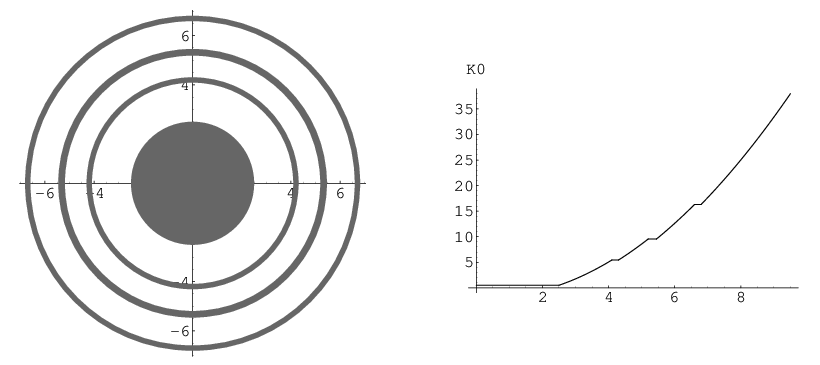
One of the simplest situations is that there are many $Z=-\frac{1}{2}~$ regions on the $z_{1}~$ plane and $z_{2}~$ plane. We can form the two-cycles between the $Z=-\frac{1}{2}~$ regions on the $z_{1}~$ plane for $D_{2}$ , and on the $z_{2}~$ plane for $\tilde{D}_{2}$ . They are the white strips in figure 1. Now we consider very thin $Z=-\frac{1}{2}~$ regions on top of the $Z=\frac{1}{2}$ background. See figure 1 for an example of thin $Z=-\frac{1}{2}~$ regions. In this case, on the $Z=\frac{1}{2}$ background, away from the very thin $Z=-\frac{1}{2}~$ regions, $\partial_{1}\bar{\partial}_{1}K_{0}|_{z_{2}=0}$ , $\partial_{2}\bar{\partial}_{2}K_{0}|_{z_{1}=0}$ are approximately given by those of the AdS expression e.g. (4.11).

We now consider the $D_{2}$ domain of $Z=\frac{1}{2}$ on $z_{1}$ plane at $z_{2}=0$ , surrounded by $Z=-\frac{1}{2}$ regions, and we have

\frac{1}{(2\pi)^{2}l_{p}^{4}}\int_{D_{2}}i\partial_{1}\bar{\partial}_{1}K_{0}dz^{1}\wedge d\bar{z}^{1}=m_{i}.

(4.12)

Similarly $\tilde{D}_{2}$ is the domain of $Z=\frac{1}{2}$ on $z_{2}~$ plane at $z_{1}=0,$ surrounded by $Z=-\frac{1}{2}~$ regions, and we have

\frac{1}{(2\pi)^{2}l_{p}^{4}}\int_{\tilde{D}_{2}}i\partial_{2}\bar{\partial}_{2}K_{0}dz^{2}\wedge d\bar{z}^{2}={\tilde{m}}_{i}.

(4.13)

According to the BPS operators in [23] expressed by the Brauer basis in [14], the operators can be labelled by two Young diagrams. These operators are briefly summarized in section 8. We may identify the flux quantum numbers $m_{i}$ with the size of the horizontal edges $m_{i}$ of the first Young diagram, and identify the flux quantum number $\ {\tilde{m}}_{i}$ with the size of the horizontal edges ${\tilde{m}}_{i}~$ of the second Young diagram. The two Young diagrams have total number of boxes $m-k$ and $n-k$ respectively,

	$\displaystyle\sum_{i}\sum_{i^{\prime}=1}^{i}m_{i^{\prime}}N_{i}$	$\displaystyle=$	$\displaystyle m-k,$		(4.14)
	$\displaystyle\sum_{i}\sum_{i^{\prime}=1}^{i}{\tilde{m}}_{i^{\prime}}\tilde{N}_{i}$	$\displaystyle=$	$\displaystyle n-k.$		(4.15)

The flux integrations at $y=0$ show how the edges of Young diagrams would be mapped, according to above discussions.

Following the earlier works, we further identify the appropriate variables and functions to characterize the geometries, and focused on the droplet space which are divided into two droplet regions, with $Z=-\frac{1}{2}$ where the $S^{3}$ vanishes and with $Z=\frac{1}{2}$ where the $S^{1}$ vanishes. The flux quantum numbers are determined by the flux integrals. The dimension of the operator is $m+n$ . Note that these are the flux quantization in the small $y$ region. These are not the same as the flux quantization in the large $r$ region.

$K_{0}$ plays an important role in these flux integrations that involve the two-cycles in the $Z=\frac{1}{2}$ regions. $K_{0}$ can be solved by the coupled equations (A.7) of $K_{0},K_{1}$ for these regions. Figure 1 shows a plot of $K_{0}$ where there are several thin $Z=-\frac{1}{2}$ strips.

Refer to caption — Figure 1: On the left side is the droplet configuration on the $z_{1}$ plane. On the right side is the plot of $K_{0}$ on the $z_{1}$ plane along the radial axis. Similarly for the $z_{2}$ plane. There are thin $Z=-\frac{1}{2}$ regions. In the limit that the thin black strips go to zero, the function goes to that of the AdS expression.

5 Droplet space, metric functions and $N_{12}$ , $M_{1}$ , $M_{2}$

5.1 Metric functions

We now study the metric functions in the geometry as well as the metric components mixing time and angles, as well as components mixing the angles. The expressions in this section are valid for all possible ranges of $z_{i}$ , $\bar{z}_{i}$ . In a different section 6, we will study their large $R$ behaviors, in the large $R$ region. We denote $R^{2}=r_{1}^{2}+r_{2}^{2}$

, and $r_{1}=\left|z_{1}\right|,r_{2}=\left|z_{2}\right|.$

We expand $K$ in powers of $y^{2}$ . The entire solutions to $K$ are determined by the functions $K_{0},K_{1},K_{2},$ see appendix A. The equations for $K$ are in Appendix A.

In this section we study exact expressions in all possible ranges of $z_{i}$ , $\bar{z}_{i}$ , but for small $y$ , since we consider $K_{0},K_{1},K_{2}$ in the series expansion in powers of $y^{2}$ .

Near $Z=1/2$ , we have the expansion

	$\displaystyle K$	$\displaystyle=$	$\displaystyle-\frac{1}{4}y^{2}\log y^{2}+K_{0}+y^{2}K_{1}+y^{4}K_{2}+y^{6}K_{3}+O(y^{8}),$		(5.1)
	$\displaystyle Z$	$\displaystyle=$	$\displaystyle\frac{1}{2}-4y^{2}K_{2}-12y^{4}K_{3}+O(y^{6}).$		(5.2)

These expressions will be used in the later derivations in this section.

We also use

\omega_{\phi_{i}}=-\frac{1}{2y}\partial_{y}(r_{i}\partial_{r_{i}}K)=-r_{i}\partial_{r_{i}}K_{1}-2y^{2}r_{i}\partial_{r_{i}}K_{2}+O(y^{4}).

(5.3)

The $\Delta$ can be expanded as

$\displaystyle\Delta$	$\displaystyle=$	$\displaystyle\frac{\mu_{3}^{2}}{r^{2}}\frac{1+2Z}{1-2Z}$	(5.4)
	$\displaystyle=$	$\displaystyle\frac{\mu_{3}^{2}}{r^{2}}\frac{1-4y^{2}K_{2}-12y^{4}K_{3}+O(y^{6})}{4y^{2}K_{2}+12y^{4}K_{3}+O(y^{6})}$
	$\displaystyle=$	$\displaystyle\frac{1}{4r^{4}K_{2}}\left(1-4y^{2}K_{2}-3y^{2}\frac{K_{3}}{K_{2}}+O(y^{4})\right).$

Note that $y=r\mu_{3}$ .

Around $y=0$ with $Z=\frac{1}{2}$ , which is approached by $\mu_{3}=0$ , we may expand it as

Z=\frac{1}{2}\frac{1-\frac{r_{0}^{2}\mu_{3}^{2}}{r^{2}\Delta}}{1+\frac{r_{0}^{2}\mu_{3}^{2}}{r^{2}\Delta}}=\frac{1}{2}-\frac{r_{0}^{2}y^{2}}{r^{4}\Delta}+\left(\frac{r_{0}^{2}y^{2}}{r^{4}\Delta}\right)^{2}+O(y^{6}).

(5.5)

Comparing (5.2),(5.5), we have

K_{2}=\frac{r_{0}^{2}}{4r^{4}\Delta}+O(y^{2}),

(5.6)

h^{2}=\sqrt{4K_{2}}+O(y^{2}).

(5.7)

5.2 Mixing components

We study particularly the important functions $M_{1},M_{2},N_{12}$ which are the mixing between time and the angles, and the mixing between the angles themselves.

We focus on the components of the geometry,

\frac{h_{ij}}{h^{2}}(d\phi_{i}+M_{i}dt)(d\phi_{j}+M_{j}dt).

(5.8)

In particular, there is also a mixing term between the angles,

2\frac{N_{12}}{h^{2}}(d\phi_{1}+M_{1}dt)(d\phi_{2}+M_{2}dt),

(5.9)

where $h_{12}=N_{12}$ .

$M_{1},M_{2}~$ account for the mixing between $t$ and $\phi_{1},\phi_{2}$ respectively. The function $N_{12}~$ account for the mixing of angles $\phi_{1}$ and $\phi_{2}.$

Using the small $y$ expansions presented in section 5.1 and $h^{2}=(1/4-Z^{2})/y^{2}$ , one can expand the $S_{i}$ , $N_{12}$ in section 2 as

$\displaystyle S_{i}$	$\displaystyle=$	$\displaystyle h^{4}S_{ii}r_{i}^{2}-\omega_{\phi_{i}}^{2}$	(5.10)
	$\displaystyle=$	$\displaystyle 2K_{2}\partial_{t_{i}}^{2}K_{0}-(\partial_{t_{i}}K_{1})^{2}+O(y^{2})$
	$\displaystyle=$	$\displaystyle s_{i}+O(y^{2})$

and

$\displaystyle N_{12}$	$\displaystyle=$	$\displaystyle h^{4}S_{12}r_{1}r_{2}-\omega_{\phi_{1}}\omega_{\phi_{2}}$	(5.11)
	$\displaystyle=$	$\displaystyle 2K_{2}\partial_{t_{1}}\partial_{t_{2}}K_{0}-(\partial_{t_{1}}K_{1})(\partial_{t_{2}}K_{1})+O(y^{2})$
	$\displaystyle=$	$\displaystyle n_{12}+O(y^{2}),$

where

$\displaystyle s_{1}$	$\displaystyle=$	$\displaystyle 2K_{2}\partial_{t_{1}}^{2}K_{0}-(\partial_{t_{1}}K_{1})^{2}$
$\displaystyle s_{2}$	$\displaystyle=$	$\displaystyle 2K_{2}\partial_{t_{2}}^{2}K_{0}-(\partial_{t_{2}}K_{1})^{2}$
$\displaystyle n_{12}$	$\displaystyle=$	$\displaystyle 2K_{2}\partial_{t_{1}}\partial_{t_{2}}K_{0}-(\partial_{t_{1}}K_{1})(\partial_{t_{2}}K_{1})$	(5.12)

have been defined. We also have introduced $t_{i}=\log r_{i}$ .³³ 3 It would be convenient to use $e^{i(\phi_{i}-\phi_{j})}\partial_{i}\partial_{\bar{j}}=\frac{1}{4r_{i}r_{j}}\partial_{t_{i}}\partial_{t_{j}}.$ It is interesting to note that only the 2nd derivatives of $K_{0}$ , and 1st derivatives of $K_{1}$ , and no derivative of $K_{2}$ appears in the expression.

Hence the mixing functions $M_{1}$ and $M_{2}$ in (2.8),(2.9) can be expanded as

	$\displaystyle M_{1}$	$\displaystyle=$	$\displaystyle-1+\frac{s_{2}\partial_{t_{1}}K_{1}-n_{12}\partial_{t_{2}}K_{1}}{s_{1}s_{2}-n_{12}^{2}}+O(y^{2}),$		(5.13)
	$\displaystyle M_{2}$	$\displaystyle=$	$\displaystyle-1+\frac{s_{1}\partial_{t_{2}}K_{1}-n_{12}\partial_{t_{1}}K_{1}}{s_{1}s_{2}-n_{12}^{2}}+O(y^{2}).$		(5.14)

These are exact expressions for any value of $r_{1},r_{2}.$ The special case of large $R^{2}(=r_{1}^{2}+r_{2}^{2})$ will be discussed in section 6.

The mixing function between the angles will be particularly important in our analysis to make a connection with the gauge theory. In general cases, it is nonzero, $n_{12}\neq 0$ . But there are special cases when $n_{12}=0$ . In this case, the $M_{i}$ becomes simpler. The special case that $n_{12}=0$ correspond to defining $N_{i}$ :

N_{i}=M_{i}|_{n_{12}=0}.

(5.15)

We find that

	$\displaystyle N_{1}$	$\displaystyle=$	$\displaystyle-1+\frac{\partial_{t_{1}}K_{1}}{s_{1}}+O(y^{2}),$		(5.16)
	$\displaystyle N_{2}$	$\displaystyle=$	$\displaystyle-1+\frac{\partial_{t_{2}}K_{1}}{s_{2}}+O(y^{2}).$		(5.17)

6 Droplet space and analysis of mixing components

We have presented general expressions for small $y$ expansions, in section 5. The geometries are parameterized by $y$ and $z_{i},\bar{z}_{i}$ . We denote $R^{2}=r_{1}^{2}+r_{2}^{2}$ , where $r_{1}=\left|z_{1}\right|,r_{2}=\left|z_{2}\right|$ . Now we analyze these expressions in the large $R$ region, by expansions in $1/R^{2}$ . We find solutions in series expansion in powers of $1/R^{2}$ . We will analyze the behavior of the mixing components $N_{12},M_{1},M_{2}$ in large $R$ .

The Kähler potential is given by the Monge-Ampere equation (A.4), and in the small $y$ expansion, the equation gives a set of equations for $K_{0}$ and $K_{1}$ [13],

(\partial_{t_{1}}\partial_{t_{1}}K_{0})(\partial_{t_{2}}\partial_{t_{2}}K_{1})+(\partial_{t_{1}}\partial_{t_{1}}K_{1})(\partial_{t_{2}}\partial_{t_{2}}K_{0})-2(\partial_{t_{1}}\partial_{t_{2}}K_{0})(\partial_{t_{1}}\partial_{t_{2}}K_{1})=0,

(6.1)

(\partial_{t_{1}}\partial_{t_{1}}K_{0})(\partial_{t_{2}}\partial_{t_{2}}K_{0})-(\partial_{t_{1}}\partial_{t_{2}}K_{0})^{2}=\frac{4}{e}e^{2t_{1}+2t_{2}}e^{2K_{1}},

(6.2)

where $t_{i}=\log r_{i}$ .

This set of the equations have some rescaling transformations:

$\displaystyle K_{0}$	$\displaystyle\rightarrow$	$\displaystyle qK_{0},$	(6.3)
$\displaystyle t_{i}$	$\displaystyle\rightarrow$	$\displaystyle\xi_{i}t_{i}+b_{i}~~\quad(r_{i}\rightarrow e^{b_{i}}(r_{i})^{\xi_{i}}),$	(6.4)
$\displaystyle K_{1}$	$\displaystyle\rightarrow$	$\displaystyle K_{1}+\log q-\sum_{i}((\xi_{i}-1)t_{i}+b_{i}+\frac{1}{2}\log\xi_{i}^{2}).$	(6.5)

Overall constant shifts in $K_{0}$ are not important because they appear with derivatives in the metric. The $\xi_{i}=-1$ transformation is the inversion transformation in [13], which exchanges small $r_{i}$ with large $r_{i}$ .

The most general form of solutions representing the $AdS_{5}\times S^{5}$ geometry, in a region with $Z=1/2$ , is ⁴⁴ 4 If we consider the following one, $K_{0}=\frac{1}{2}(a(r_{1}^{2}+r_{2}^{2}))-\frac{q}{2}\log(a(sr_{1}^{2}+r_{2}^{2})),$ the equations require $s=1$ .

K_{0}=\frac{1}{2}(a(sr_{1}^{m}+r_{2}^{n}))-\frac{q}{2}\log(a(sr_{1}^{m}+r_{2}^{n})).

(6.6)

Using the rescaling transforms, this may be brought to the simplest form $K_{0}=\frac{1}{2}R^{2}-\frac{1}{2}\log R^{2}$ , where $R^{2}=r_{1}^{2}+r_{2}^{2}$ . In our analysis, parameters $a,q$ will be reserved to account for the possible scaling transformation for $R$ (or $z_{i},\bar{z}_{i}$ ) and $K$ .

For example, we can have the rescaling transformations:

$\displaystyle K_{0}$	$\displaystyle\rightarrow$	$\displaystyle qK_{0},$	(6.7)
$\displaystyle\frac{q}{a}R^{2}$	$\displaystyle\rightarrow$	$\displaystyle R^{2},$	(6.8)
$\displaystyle sr_{1}^{2}$	$\displaystyle\rightarrow$	$\displaystyle r_{1}^{2},$	(6.9)

together with constant shifts of $K_{1}$ , and rescaling of $y$ .

We are interested in more general solutions. We will first consider from large $R$ point of view. In the large $R$ , we have that, $r^{2}=aR^{2}(1+O(1/r^{2}))+O(y^{2})$ , so in the region where $R$ is large, we have that $r$ is also large.

We denote $R^{2}=r_{1}^{2}+r_{2}^{2}$ . Note that $aR^{2},ar_{1}^{2},ar_{2}^{2}$ often appear in combinations in their products, due to that $\sqrt{a}$ rescales the $r_{i}$ coordinates, as in (6.8).

We find a family of expressions that satisfy the set of the equations, as follows:

$K_{0}$ is given by

K_{0}=\frac{1}{2}aR^{2}-\frac{1}{2}q\log(aR^{2})+K_{0}^{(1)},

(6.10)

$\displaystyle\partial_{t_{1}}^{2}K_{0}$	$\displaystyle=$	$\displaystyle 2ar_{1}^{2}\left(1-\frac{qr_{2}^{2}}{aR^{4}}+O(1/r^{4})\right),$	(6.11)
$\displaystyle\partial_{t_{2}}^{2}K_{0}$	$\displaystyle=$	$\displaystyle 2ar_{2}^{2}\left(1-\frac{qr_{1}^{2}}{aR^{4}}+O(1/r^{4})\right),$	(6.12)
$\displaystyle\partial_{t_{1}}\partial_{t_{2}}K_{0}$	$\displaystyle=$	$\displaystyle\frac{2qr_{1}^{2}r_{2}^{2}}{R^{4}}\left(1+\frac{q\alpha_{0}}{aR^{2}}+O(1/r^{4})\right),$	(6.13)

and $K_{1}$ is

K_{1}=\frac{1}{2}\log\left(\frac{a\left(aR^{2}-q\right)}{R^{2}}\right)+\frac{1}{2}+K_{1}^{(1)},

(6.14)

	$\displaystyle\partial_{t_{1}}K_{1}$	$\displaystyle=$	$\displaystyle\frac{qr_{1}^{2}}{aR^{4}}\left(1+\frac{q}{aR^{2}}(1+\kappa_{1})+O(1/r^{4})\right),$		(6.15)
	$\displaystyle\partial_{t_{2}}K_{1}$	$\displaystyle=$	$\displaystyle\frac{qr_{2}^{2}}{aR^{4}}\left(1+\frac{q}{aR^{2}}(1+\kappa_{2})+O(1/r^{4})\right),$		(6.16)

and $K_{2}$ is

	$\displaystyle K_{2}$	$\displaystyle=$	$\displaystyle\frac{q}{4(aR^{2}-q)^{2}}+K_{2}^{(1)}$		(6.17)
		$\displaystyle=$	$\displaystyle\frac{q}{4a^{2}R^{4}}\left(1+\frac{q}{aR^{2}}(2+\alpha_{2})+O(1/r^{4})\right).$		(6.18)

The expressions without $K_{0}^{(1)},K_{1}^{(1)},K_{2}^{(1)}$ is the solution for AdS (see [13] for other related analysis). $K_{0}^{(1)},K_{1}^{(1)},K_{2}^{(1)}$ are deviations from AdS. The $\alpha_{0}$ , $\kappa_{1}$ , $\kappa_{2}$ , $\alpha_{2}~$ are the effect of turning on $K_{0}^{(1)},K_{1}^{(1)},K_{2}^{(1)}$ . In the second lines in (6.13),(6.15),(6.16),(6.18), the large $r$ expansion with the effect of $K_{0}^{(1)},K_{1}^{(1)},K_{2}^{(1)}$ are given.

From the differential equations, we find a family of $K^{(1)}$ ,

$\displaystyle K_{0}^{(1)}$	$\displaystyle=$	$\displaystyle\frac{q^{2}}{a}\left(\frac{dr_{1}^{2}+er_{2}^{2}}{R^{4}}+O(1/r^{4})\right),\quad$	(6.19)
$\displaystyle K_{1}^{(1)}$	$\displaystyle=$	$\displaystyle-\frac{q^{2}}{a^{2}R^{2}}\left(\frac{(d-e)(r_{1}^{2}-r_{2}^{2})}{R^{4}}+O(1/r^{4})\right),$	(6.20)
$\displaystyle K_{2}^{(1)}$	$\displaystyle=$	$\displaystyle\frac{q^{2}}{4a^{3}R^{6}}\left(c-2(d+e)+\frac{6(d-e)(r_{1}^{2}-r_{2}^{2})}{R^{2}}\right)+\frac{q^{2}}{4a^{2}R^{4}}O(1/r^{4}).$	(6.21)

We note that three parameters $c$ , $d$ , $e$ have come in, and they will be identified with the three parameters $m,n,k$ of Young diagrams in (8.2).

These solutions give that in (6.13),(6.15),(6.16),(6.18),

$\displaystyle\alpha_{0}$	$\displaystyle=$	$\displaystyle 2(d+e)+\frac{6(d-e)(r_{1}^{2}-r_{2}^{2})}{R^{2}},$
$\displaystyle\alpha_{2}$	$\displaystyle=$	$\displaystyle\alpha_{0}+c-4(d+e),$
$\displaystyle\kappa_{1}$	$\displaystyle=$	$\displaystyle\alpha_{0}-4d,$
$\displaystyle\kappa_{2}$	$\displaystyle=$	$\displaystyle\alpha_{0}-4e.$	(6.22)

Now we evaluate the $N_{12},M_{1},M_{2}$ in the large $r$ region, using the general expressions (5.11),(5.13),(5.14), as follows:

$\displaystyle N_{12}$	$\displaystyle=$	$\displaystyle 2K_{2}\partial_{t_{1}}\partial_{t_{2}}K_{0}-\partial_{t_{1}}K_{1}\partial_{t_{2}}K_{1}+O(y^{2})$	(6.23)
	$\displaystyle=$	$\displaystyle\frac{r_{1}^{2}r_{2}^{2}}{a^{2}R^{8}}\frac{q^{3}}{aR^{2}}\left(\alpha_{0}+\alpha_{2}-\kappa_{1}-\kappa_{2}\right)+O(1/r^{8})+O(y^{2})$
	$\displaystyle=$	$\displaystyle\frac{q^{3}\mu_{1}^{2}\mu_{2}^{2}}{r^{6}}k+O(1/r^{8})+O(y^{2}),$

$\displaystyle M_{1}$	$\displaystyle=$	$\displaystyle-1+\frac{s_{2}\partial_{t_{1}}K_{1}-n_{12}\partial_{t_{2}}K_{1}}{s_{1}s_{2}-n_{12}^{2}}+O(y^{2})$	(6.24)
	$\displaystyle=$	$\displaystyle\frac{q}{aR^{2}}\left(-\alpha_{2}+\kappa_{1}\right)+O(1/r^{4})+O(y^{2})$
	$\displaystyle=$	$\displaystyle-\frac{qm}{r^{2}}+O(1/r^{4})+O(y^{2}),$

and

$\displaystyle M_{2}$	$\displaystyle=$	$\displaystyle-1+\frac{s_{1}\partial_{t_{2}}K_{1}-n_{12}\partial_{t_{1}}K_{1}}{s_{1}s_{2}-n_{12}^{2}}+O(y^{2})$	(6.25)
	$\displaystyle=$	$\displaystyle\frac{q}{aR^{2}}\left(-\alpha_{2}+\kappa_{2}\right)+O(1/r^{4})+O(y^{2})$
	$\displaystyle=$	$\displaystyle-\frac{qn}{r^{2}}+O(1/r^{4})+O(y^{2}),$

where we identify $r^{2}=aR^{2}(1+O(1/r^{2}))+O(y^{2})$ and $\frac{1}{r^{2}}=\frac{1}{aR^{2}}(1+O(1/r^{2}))+O(y^{2})$ . We are making expansions in power series of $y^{2}$ and $~1/r^{2}.$ More details of the above derivations are in Appendix C.

In the expression of $M_{1}$ , $M_{2}$ , we have identified

	$\displaystyle q\left(\alpha_{2}-\kappa_{1}\right)$	$\displaystyle=$	$\displaystyle qm=q_{1},$		(6.26)
	$\displaystyle q\left(\alpha_{2}-\kappa_{2}\right)$	$\displaystyle=$	$\displaystyle qn=q_{2}.$		(6.27)

In the large $r$ , we have the quantization of electric charges by

$\displaystyle A^{i}$	$\displaystyle=$	$\displaystyle M_{i}dt,$	(6.28)
$\displaystyle F_{(2)}^{1}$	$\displaystyle=$	$\displaystyle dM_{1}dt=drdt\left(\frac{2q}{r^{3}}m+O(1/r^{5})\right),$	(6.29)
$\displaystyle F_{(2)}^{2}$	$\displaystyle=$	$\displaystyle dM_{2}dt=drdt\left(\frac{2q}{r^{3}}n+O(1/r^{5})\right),$	(6.30)

	$\displaystyle\frac{1}{4\pi^{2}}\int\ast F_{(2)}^{1}$	$\displaystyle=$	$\displaystyle m,$		(6.31)
	$\displaystyle\frac{1}{4\pi^{2}}\int\ast F_{(2)}^{2}$	$\displaystyle=$	$\displaystyle n,$		(6.32)

where in our coordinates $g_{tt}g_{rr}=q$ in large $r$ , and where $m,n$ are the two charges. Note that terms corresponding to $O(1/r^{4})$ in (6.24),(6.25) will not contribute to the integral.

In the expression of $N_{12}$ , we have identified

\alpha_{0}+\alpha_{2}-\kappa_{1}-\kappa_{2}=k.

(6.33)

The two angles are the angles in the $z_{1}$ plane and $z_{2}$ plane respectively.

This $k$ will be identified with the $k$ parameter in the Brauer algebra representation.

In other words, for nonzero $k$ ,

N_{12}=k\frac{\mu_{1}^{2}\mu_{2}^{2}q^{3}}{r^{6}}+O(1/r^{8}).

(6.34)

It appears at order $1/r^{6}$ with coefficients $k.$ For the special case $k=0,$ it may appear at only order $1/r^{8}.~$ See Appendix C for more details. The difference between $M_{i}$ and $N_{i}~$ is order $k/r^{4}$ for nonzero $k$ , and $1/r^{6}$ for zero $k$ .

Plugging these relations (6.26),(6.27),(6.33)

into the solutions (6.22), we find

$\displaystyle 4e$	$\displaystyle=$	$\displaystyle k-m=k-q_{1}/q,$
$\displaystyle 4d$	$\displaystyle=$	$\displaystyle k-n=k-q_{2}/q,$
$\displaystyle c$	$\displaystyle=$	$\displaystyle k.$	(6.35)

Note that in this family of solutions, the coefficients $e\leqslant 0,d\leqslant 0$ amount to that $k-m\leqslant 0,k-n\leqslant 0.$ Therefore the sign property of $e,d$ , which are either negative or zero, imposes the constraints $k\leqslant m,n$ , or equivalently $k\leqslant\min(m,n).$

In the $y$ expansions, we have, from (6.22),

$\displaystyle q\alpha_{0}$	$\displaystyle=$	$\displaystyle qk+3q_{1}\mu_{1}^{2}+3q_{2}\mu_{2}^{2}-2q_{1}-2q_{2},$	(6.36)
$\displaystyle q\alpha_{2}$	$\displaystyle=$	$\displaystyle 3q_{1}\mu_{1}^{2}+3q_{2}\mu_{2}^{2}-q_{1}-q_{2},$	(6.37)
$\displaystyle q\kappa_{1}$	$\displaystyle=$	$\displaystyle 3q_{1}\mu_{1}^{2}+3q_{2}\mu_{2}^{2}-2q_{1}-q_{2},$	(6.38)
$\displaystyle q\kappa_{2}$	$\displaystyle=$	$\displaystyle 3q_{1}\mu_{1}^{2}+3q_{2}\mu_{2}^{2}-q_{1}-2q_{2},$	(6.39)

where we used that $\mu_{1}^{2}+\mu_{2}^{2}=1-y^{2}/r^{2}=1-O(y^{2}).$

There are several equivalent and alternative ways of writing these variables, see Appendix C for more details. For example,

qk=q\alpha_{0}-q\alpha_{2}+q_{1}+q_{2}=q\alpha_{0}+q\alpha_{2}-q\kappa_{1}-q\kappa_{2},

(6.40)

which will be frequently used in the derivations.

7 Droplets and Young diagram operators

Now we turn to the analysis of the droplet configurations. The solutions in section 6 are the large $R$ expressions that result from the droplet configurations. The solution in section 6 are in the large $R$ region of the full solution in all the ranges of $z_{i}$ , $\bar{z}_{i}$ . In this section, we also provide further duality relation with the operators labelled by Brauer algebra.

We have that from section 6,

K_{0}=\frac{1}{2}aR^{2}-\frac{q}{2}\log(aR^{2})+\frac{q^{2}}{a}\left(\frac{(d+e)}{2R^{2}}+\frac{(d-e)(r_{1}^{2}-r_{2}^{2})}{2R^{4}}+O(1/r^{4})\right)

(7.1)

in large $R$ , and where

	$\displaystyle-4d$	$\displaystyle=$	$\displaystyle n-k,~~\ \ \ \ \$		(7.2)
	$\displaystyle-4e$	$\displaystyle=$	$\displaystyle m-k.\$		(7.3)

As in section 4, e.g. (4.3), the flux quantization requires that the total droplet volume to be quantized,

\int_{\mathcal{D}}d^{2}z_{1}^{\prime}d^{2}z_{2}^{\prime}=\int_{\mathcal{D}(\emptyset)}d^{2}z_{1}^{\prime}d^{2}z_{2}^{\prime}=2\pi^{3}l_{p}^{4}N

(7.4)

where $\mathcal{D}$ is the total $Z=-\frac{1}{2}$ droplets. Here we use the notation that $d^{2}z_{1}d^{2}z_{2}=dx_{1}dx_{2}dx_{3}dx_{4}$ for convenience. $\mathcal{D}(\emptyset)$ is the $Z=-\frac{1}{2}~$ configuration such that there is no any finite $Z=\frac{1}{2}~$ domains or $Z=\frac{1}{2}$ bubbles. In the large $R$ , it was shown [13] that, if we expand

K_{0}=\frac{1}{2}a(\left|z_{1}\right|^{2}+\left|z_{2}\right|^{2})+\widetilde{K}_{0},\qquad K_{1}=\frac{1}{2}+\widetilde{K}_{1},

(7.5)

	$\displaystyle\frac{1}{a}\partial_{1}\partial_{\bar{1}}\widetilde{K}_{0}+\partial_{2}\partial_{\bar{2}}\widetilde{K}_{0}=\widetilde{K}_{1},$		(7.6)
	$\displaystyle\partial_{1}\partial_{\bar{1}}\widetilde{K}_{1}+\partial_{2}\partial_{\bar{2}}\widetilde{K}_{1}=0.$		(7.7)

This means that a general solution to $\widetilde{K}_{0}$ is $-\frac{1}{2}\log(a\left|z_{1}-z_{1}^{\prime}\right|^{2}+a\left|z_{2}-z_{2}^{\prime}\right|^{2})$ with ( $z_{1}^{\prime}$ , $\bar{z}_{1}^{\prime}$ , $z_{2}^{\prime}$ , $\bar{z}_{2}^{\prime}$ ) arbitrary, therefore we can approximately expand $K_{0}$ as

	$\displaystyle K_{0}=\frac{1}{2}aR^{2}-\frac{q}{2}\log(aR^{2})-\frac{q}{4\pi^{3}l_{p}^{4}N}\int_{\mathcal{D}}d^{2}z_{1}^{\prime}d^{2}z_{2}^{\prime}\log(a\left\|z_{1}-z_{1}^{\prime}\right\|^{2}+a\left\|z_{2}-z_{2}^{\prime}\right\|^{2})$
	$\displaystyle+\frac{q}{4\pi^{3}l_{p}^{4}N}\int_{\mathcal{D}(\emptyset)}d^{2}z_{1}^{\prime}d^{2}z_{2}^{\prime}\log(a\left\|z_{1}-z_{1}^{\prime}\right\|^{2}+a\left\|z_{2}-z_{2}^{\prime}\right\|^{2})+O(1/R^{4}).$		(7.8)

Both (7.1),(7.8) satisfy the equations (7.6),(7.7). The droplet configuration in $\mathcal{D}$ gives nontrivially the information of $d,e$ in the large $R$ , when comparing two expressions (7.1),(7.8).

Suppose we consider configurations that only depend on $r_{1},r_{2}$ , and in the case when $d$ and $e$ are equal, where there are more symmetry in the droplet configuration, we can expand

(7.8),

\displaystyle K_{0}

\displaystyle=

\displaystyle\frac{1}{2}aR^{2}-\frac{q}{2}\log(aR^{2})-\frac{q(M_{{}_{11}}^{\left[2\right]}-M_{{}_{11,\emptyset}}^{\left[2\right]})}{4\pi^{3}l_{p}^{4}NR^{2}}-\frac{q(M_{{}_{22}}^{\left[2\right]}-M_{{}_{22,,\emptyset}}^{\left[2\right]})}{4\pi^{3}l_{p}^{4}NR^{2}}+O(1/R^{4})

where

	$\displaystyle M_{{}_{11}}^{\left[2\right]}-M_{{}_{11,\emptyset}}^{\left[2\right]}$	$\displaystyle=$	$\displaystyle\int_{\mathcal{D}}d^{2}z_{1}^{\prime}d^{2}z_{2}^{\prime}\left\|z_{1}^{\prime}\right\|^{2}-\int_{\mathcal{D}(\emptyset)}d^{2}z_{1}^{\prime}d^{2}z_{2}^{\prime}\left\|z_{1}^{\prime}\right\|^{2},$		(7.10)
	$\displaystyle M_{{}_{22}}^{\left[2\right]}-M_{{}_{22,\emptyset}}^{\left[2\right]}$	$\displaystyle=$	$\displaystyle\int_{\mathcal{D}}d^{2}z_{1}^{\prime}d^{2}z_{2}^{\prime}\left\|z_{2}^{\prime}\right\|^{2}-\int_{\mathcal{D}(\emptyset)}d^{2}z_{1}^{\prime}d^{2}z_{2}^{\prime}\left\|z_{2}^{\prime}\right\|^{2},$		(7.11)

are the second moments along the axis perpendicular to $z_{1}$ plane and $z_{2}$ plane respectively, subtracted from those of the configuration without any finite $Z=\frac{1}{2}$ domains. The crossing terms $z_{i}\bar{z}_{i}^{\prime}$ cancels due to symmetric configuration in $z_{1}$ plane and in $z_{2}$ plane.

We read off the coefficients that

			$\displaystyle\frac{1}{2\pi^{3}l_{p}^{4}N}(M_{{}_{11}}^{\left[2\right]}-M_{{}_{11,\emptyset}}^{\left[2\right]})+\frac{1}{2\pi^{3}l_{p}^{4}N}(M_{{}_{22}}^{\left[2\right]}-M_{{}_{22,\emptyset}}^{\left[2\right]})$		(7.12)
		$\displaystyle=$	$\displaystyle\frac{1}{4}\frac{q}{a}[(n-k)+(m-k)]=-\frac{q}{a}(d+e).$		(7.13)

If we use the convention $\frac{q}{a}=r_{0}^{2}=(4\pi l_{p}^{4}N)^{1/2}$ e.g. as from (4.5), and in the unit $r_{0}=1,$

(M_{{}_{11}}^{\left[2\right]}-M_{{}_{11,\emptyset}}^{\left[2\right]})+(M_{{}_{22}}^{\left[2\right]}-M_{{}_{22,\emptyset}}^{\left[2\right]})=\frac{\pi^{2}}{8}[(n-k)+(m-k)].

(7.14)

We then identify the second moments in two directions,

	$\displaystyle(M_{{}_{11}}^{\left[2\right]}-M_{{}_{11,\emptyset}}^{\left[2\right]})$	$\displaystyle=$	$\displaystyle\frac{\pi^{2}}{8}(n-k),$		(7.15)
	$\displaystyle(M_{{}_{22}}^{\left[2\right]}-M_{{}_{22,\emptyset}}^{\left[2\right]})$	$\displaystyle=$	$\displaystyle\frac{\pi^{2}}{8}(m-k),$		(7.16)

where we are in the unit $r_{0}=1$ .

Note that we also have the relation, from section 4,

	$\displaystyle\sum_{i}\sum_{i^{\prime}=1}^{i}m_{i^{\prime}}N_{i}$	$\displaystyle=$	$\displaystyle m-k,$		(7.17)
	$\displaystyle\sum_{i}\sum_{i^{\prime}=1}^{i}{\tilde{m}}_{i^{\prime}}\tilde{N}_{i}$	$\displaystyle=$	$\displaystyle n-k.$		(7.18)

The change in the potential $K_{0}$ is negative, when increasing the second moments. It is analogous to the change of the potential from $-\log R^{2}$ to $-\log(R^{2}+\delta^{2}$ ), due to increased second moments. So the signs of $d,e$ are negative or zero in the above expression, that is

d\leqslant 0,\,\,\,\,e\leqslant 0.

(7.19)

This sign property can be understood as that the potential in (7.8) will decrease when the $Z=-\frac{1}{2}$ droplets in the droplet space are more outwards. The droplet second moments are increased from those of the configuration when there is no any finite $Z=\frac{1}{2}~$ domains. The condition (7.19) is consistent with

\vskip 1.0pt(M_{{}_{11}}^{\left[2\right]}-M_{{}_{11,\emptyset}}^{\left[2\right]})\geqslant 0,\,\,\,(M_{{}_{22}}^{\left[2\right]}-M_{{}_{22,\emptyset}}^{\left[2\right]})\geqslant 0.

(7.20)

This amounts to

m-k\geqslant 0,\,\,\,\,n-k\geqslant 0

(7.21)

or equivalently

k\leqslant\min(m,n)

(7.22)

from the gravity side.

The dual operator has dimension $m+n,$ and the two Young diagrams have $m-k$ and $n-k$ boxes respectively. The dimension is larger than the total number of boxes by the amount $2k$ . The $k$ parameter is identified in the last section as in (6.23),(6.33) as due to the mixing of two angular directions. The two angles are the angles in the $z_{1}$ plane and $z_{2}$ plane respectively. We see that $2k$ measures the energy excess over the total number of boxes, and is accounted for by the mixing of two angular directions in the situation described here.

The total number of boxes match the calculation from the flux quantum numbers, as $m-k$ and $n-k$ for two two-planes.

The Brauer algebra provides two Young diagram representations, and each correspond to droplet configurations in $z_{1}$ and $z_{2}$ planes respectively. For example, for configurations that have $2l_{1}$ concentric circles in the droplet plane $z_{1}$ , this configuration maps to the $2l_{1}$ edges of the first Young diagram $\gamma_{+}$ , and the flux quantization numbers on each droplet region map to the lengths of the edges of the Young diagram $\gamma_{+}$ . There are also $2l_{2}$ concentric circles in the droplet plane $z_{2}$ , and this configuration maps to the $2l_{2}$ edges of the second Young diagram $\gamma_{-}$ , and the flux quantization numbers on each droplet region map to the lengths of the edges of the Young diagram $\gamma_{-}$ . See figure 2. These two Young diagrams are depicted in figures 2(d), 2(e) in the example.

We can characterize the droplet configuration by three diagrams, for those depending only on $r_{1},r_{2}.$ The first two diagrams are concentric ring patterns of alternative $Z=\frac{1}{2}$ and $Z=-\frac{1}{2}$ regions in $z_{1}$ planes and in $z_{2}$ planes, see figures 2(a), 2(b) for example. The third diagram is a diagram in the $(r_{1},r_{2})$ quadrant, see figure 2(c).

We first map the corners in two Young diagrams to ordered points along $r_{1},r_{2}$ axis respectively in figure 2(c). Then we draw diagrams connecting ordered points along $r_{1}$ axis to those along $r_{2}~$ axis, dividing regions in $(r_{1},r_{2})$ space into $Z=-\frac{1}{2}$ (depicted in black) and $Z=\frac{1}{2}$ (depicted in white).

We can also draw more complicated droplets. In the gravity description, when we draw the lines, there are extra possibilities for possible lines to go in the middle region of $(r_{1},r_{2})$ space. These may correspond to other operators that are superpositions of the Brauer basis.

For those configurations that depend not only on $r_{1},r_{2}$ , they could be the superpositions of the Young diagram operators in the above discussions. For example, one can add small ripples on any boundaries of the droplets. See also related discussions, e.g. [18]. The configurations that correspond to ripples on the droplet boundaries, can be considered as the superpositions of the Young diagram operators in the above discussions.

In [10], 1/2 BPS geometries were uplifted into the systems of 1/4 and 1/8 BPS geometries, and there are disconnected droplets with various topologies in 4d or 6d droplet space respectively, and the topology change transitions occurred in [6],[19] uplift to the topology change transitions in 4d and 6d. In general, in the 4d droplet space we study here, the topology change transition happens commonly.

The condition (7.22) is consistent with the range of $k$ in Brauer algebra representation. The droplet information are encoded in the Young diagrams. There is correspondence between the pair of Young diagrams and the concentric droplet configuration in the two complex planes. The operators labelled by the Young diagrams of Brauer algebra give a family of globally well-defined spacetime geometries. Other bases may also be related to the droplet picture, since they can be related by transformations, and it might be interesting to see how $k$ is produced in other bases. The system of geometries are dual to the system of the corresponding operators.

8 Gauge invariant operators by Brauer algebra

Now we will briefly summarize the operators based on the Brauer algebra [14],[22]. See also related discussion in [30],[31].

We take two complex fields $X$ , $Y$ out of three complex fields and consider gauge invariant operators constructed from $m$ $X$ s and $n$ $Y$ s. The $U(N)$ gauge group is considered. The operators are conveniently expressed in the notation of [14],[22] by

O_{A,ij}^{\gamma}(X,Y)=tr_{m,n}\left(Q_{A,ij}^{\gamma}X^{\otimes m}\otimes(Y^{T})^{\otimes n}\right),

(8.1)

where $Q_{A,ij}^{\gamma}$ is given by a linear combination of elements in the Brauer algebra. Irreducible representations of the Brauer algebra are denoted by $\gamma$ , which are given by two Young diagrams:

\gamma=(\gamma_{+},\gamma_{-}),

(8.2)

where $\gamma_{+}$ is a Young diagram with $m-k$ boxes and $\gamma_{-}$ is a Young diagram with $n-k$ boxes. $k$ is an integer satisfying $0\leqslant k\leqslant\min(m,n)$ . $A=(R,S)$ is an irreducible representation of $S_{m}\times S_{n}$ , labelled by two Young diagrams with $m$ and $n$ boxes. $i,j$ are multiplicity indices with respect to the embedding of $A$ into $\gamma$ .

An advantage of this basis is that the free two-point functions are diagonal. We also note that non-planar corrections are fully taken into account.

Because the number of boxes in $\gamma$ is characterized by $k$ , it is convenient to classify the operators by the integer $k$ .

The labels can be simplified when $k=0$ , because $i,j$ are trivial, and we have $\gamma_{+}=R$ , $\gamma_{-}=S$ . Hence the operators in $k=0$ are labelled by two Young diagrams. Denoting $P_{R,S}=Q_{A,ij}^{\gamma(k=0)}$ , the expression in (8.1) becomes

O_{R,S}(X,Y)=tr_{m,n}\left(P_{R,S}X^{\otimes m}\otimes(Y^{T})^{\otimes n}\right).

(8.3)

In this sector, the operators have the nice expansion with respect to $1/N$ , whose leading term is given by

O_{R,S}(X,Y)=O_{R}(X)O_{S}(Y)+\cdots.

(8.4)

Here $O_{R}(X)$ is the Schur polynomial built from the $X$ fields labelled by a Young diagram $R$ with $m$ boxes, and $O_{S}(Y)$ is the Schur polynomial built from the $Y$ fields labelled by a Young diagram $S$ with $n$ boxes.

In general, including the case $k=0$ , the leading term of the operators (8.1) looks schematically like

O_{A,ij}^{\gamma}(X,Y)\sim tr_{m,n}\left(\sigma C^{k}X^{\otimes m}\otimes(Y^{T})^{\otimes n}\right)+\cdots,

(8.5)

where $\sigma$ is an element in $S_{m}\times S_{n}$ and $C$ is an operation contracting the upper index of an $X$ and the upper index of a $Y^{T}$ . Each term in the dots in the above expression (8.5) contains more contractions. In other words, $k$ is the minimum number of contractions involved in the $Q_{A,ij}^{\gamma}$ of an operator. Therefore the $k$ can be given the intuitive meaning that it measures the degree of the mixing between the two fields. For example, the $k=0$ has no mixing in the sense of (8.4). The opposite case is the case $k$ takes the maximum value. With the condition $m=n$ , operators in $k=m=n$ are found to be expressed by operators of the combined matrix $XY$ [31].

In the paper [23], a class of the $1/4$ BPS operators were constructed by exploiting algebraic properties of the Brauer algebra, where it was shown that the operators $O_{R,S}(X,Y)$ and $\sum_{R,S,i}O_{A,ii}^{\gamma\hskip 1.42271pt(k\neq 0)}(X,Y)$ are annihilated by the one-loop dilatation operator, for any $m$ , $n$ and $N$ . Defining $P^{\gamma}=\sum_{A,i}Q_{A,ii}^{\gamma}$ for $k\neq 0$ , the BPS operators are presented by

O^{\gamma}(X,Y)=tr_{m,n}(P^{\gamma}X^{\otimes m}\otimes(Y^{T})^{\otimes n})

(8.6)

for both $k=0$ and $k\neq 0$ . Note that $P^{\gamma}$ is the projector associated with an irreducible representation $\gamma$ of the Brauer algebra.

It is interesting to find that they are labelled by two Young diagrams with boxes whose total number depends on the integer $k$ for fixed $m$ and $n$ . In $k=0$ , the number of boxes involved in a representation $\gamma$ is equal to the sum of the R-charges. On the other hand, when $k$ is non-zero, the Young diagrams $\gamma=(\gamma_{+},\gamma_{-})$ have a smaller number of boxes than the sum of the R-charges. The number of the deficit boxes in the $\gamma$ is $2k$ .

When $k$ is equal to $n$ for $m\geqslant n$ , the operators are labelled by a single Young diagram with $m-k$ boxes. A special case happens for $k=m$ with $m=n$ . The operator does not have any Young diagrams, but this is different from the case $m=n=0$ . For a given $m=n$ , there is only one 1/4 BPS operator labelled by the trivial representation.

We now have a remark on a constraint for representations of the Brauer algebra. The representations $\gamma$ have the constraint $c_{1}(\gamma_{+})+c_{1}(\gamma_{-})\leq N$ , where $c_{1}$ denotes the length of the first column of the Young diagram. More explanations are provided in [14]. This constraint is consistent with the identifications in sections 4 and 7.

The Brauer basis can be used in various ways. One of the motivations of constructing the Brauer basis in [14] was to construct an operator describing a set of D-branes and anti-D-branes, which is realized as the $k=0$ sector. In the application of the Brauer basis to the $su(2)$ sector, which is relevant for the present work, the $k=0$ sector realizes natural operators dual to the objects with two fields. Furthermore the construction of the basis introduces the operators labelled by $k\neq 0$ as well. In the mapping proposed in this paper, the quantum number $k$ has been given a meaning as the mixing between the two angular directions from the gravity point of view. The use of the Brauer algebra may be rephrased as the manifestation of such a good quantum number.

On the other hand, the BPS operators may be described by other bases diagonalizing free two-point functions, as in [15],[16], see also related discussions, [36],[32],[34],[35], [33]. Because other bases respect other quantum numbers, understanding a map between the two sides for other bases could also be useful for getting a complete duality of this sector.

9 Asymptotics of metric

In this section we analyze the large $r$ asymptotics of the geometry. We start from the expression (2.4). The large $r$ region includes the large $R$ region of the droplet space. We first expand in small $y$ , and have $K_{0},K_{1},K_{2}$ . We then expand these functions in powers of $1/r^{2}$ . In the large $r$ , we have

\frac{r_{1}^{2}}{R^{2}}=\mu_{1}^{2}\left(1+O(1/r^{2})\right),~~~~\frac{r_{2}^{2}}{R^{2}}=\mu_{2}^{2}\left(1+O(1/r^{2})\right),

(9.1)

R_{1}=\frac{1}{\sqrt{a}}\sqrt{r^{2}+qC_{1}}\left(1+O(1/r^{2})\right),\quad R_{2}=\frac{1}{\sqrt{a}}\sqrt{r^{2}+qC_{2}}\left(1+O(1/r^{2})\right).

(9.2)

Near $y=0$ , but large $R$ , from (5.4),

$\displaystyle\Delta$	$\displaystyle=$	$\displaystyle\frac{1}{4r^{4}K_{2}}+O(y^{2})$	(9.3)
	$\displaystyle=$	$\displaystyle\frac{a^{2}R^{4}}{r^{4}q}\left(1-\frac{q(2+\alpha_{2})}{aR^{2}}+O(1/r^{4})\right)+O(y^{2})$
	$\displaystyle=$	$\displaystyle\frac{1}{q}\left(1+\frac{q(2C_{i}\mu_{i}^{2}-2-\alpha_{2})}{r^{2}}\right)+O(1/r^{4})+O(y^{2})$
	$\displaystyle=$	$\displaystyle\frac{1}{q}\left(1+\frac{q(q_{1}+q_{2}-q_{1}\mu_{1}^{2}-q_{2}\mu_{2}^{2})}{r^{2}}\right)+O(1/r^{4})+O(y^{2})$

where we have used (6.37) and have identified

qC_{1}=q+q_{1},\quad qC_{2}=q+q_{2}.

(9.4)

We find that $\Delta$ has the same asymptotic form as the two-charge superstar.

The asymptotic form of the metric can be rewritten in the following form

ds^{2}=\sqrt{\Delta}ds_{1}^{2}+\frac{1}{\sqrt{\Delta}}ds_{2}^{2}

(9.5)

analogous to the gauged supergravity ansatz. We have that

	$\displaystyle ds_{1}^{2}$	$\displaystyle=$	$\displaystyle-\left(r^{2}+q-\frac{q^{2}(C_{1}\mu_{1}^{2}+C_{2}\mu_{2}^{2}-1+\alpha_{2}-2\kappa_{1}\mu_{1}^{2}-2\kappa_{2}\mu_{2}^{2})}{r^{2}}+O(1/r^{4})\right)dt^{2}$		(9.6)
			$\displaystyle+\frac{q}{r^{2}}\left(1-\frac{q(3C_{1}\mu_{1}^{2}+3C_{2}\mu_{2}^{2}-\alpha_{2}-2)}{r^{2}}+O(1/r^{4})\right)dr^{2}+r^{2}d\Omega_{3}^{2}$		(9.6)

and

$\displaystyle ds_{2}^{2}$	$\displaystyle=$	$\displaystyle d\mu_{3}^{2}+\mu_{3}^{2}d\psi^{2}+H_{1}\left[d\mu_{1}^{2}+\mu_{1}^{2}\left(1+O(1/r^{4})\right)(d\phi_{1}+M_{\phi_{1}}dt)^{2}\right]$
		$\displaystyle+H_{2}\left[d\mu_{2}^{2}+\mu_{2}^{2}\left(1+O(1/r^{4})\right)(d\phi_{2}+M_{\phi_{2}}dt)^{2}\right]$
		$\displaystyle+O(1/r^{5})d\mu_{1}dr+O(1/r^{5})d\mu_{2}dr$
		$\displaystyle+2\frac{q^{2}}{r^{4}}(C_{1}+C_{2}+\alpha_{0}-\alpha_{2}-2)(1+O(1/r^{2}))\mu_{1}\mu_{2}d\mu_{1}d\mu_{2}$
		$\displaystyle+2\frac{q^{2}\mu_{1}^{2}\mu_{2}^{2}}{r^{4}}(\alpha_{2}+\alpha_{0}-\kappa_{1}-\kappa_{2})(1+O(1/r^{2}))(d\phi_{1}+M_{\phi_{1}}dt)(d\phi_{2}+M_{\phi_{2}}dt)$

where the $M_{i}$ were calculated in the section 6,

	$\displaystyle M_{1}=\frac{q}{r^{2}}(-\alpha_{2}+\kappa_{1})+O(1/r^{4})+O(y^{2}),$		(9.8)
	$\displaystyle M_{2}=\frac{q}{r^{2}}(-\alpha_{2}+\kappa_{2})+O(1/r^{4})+O(y^{2}).$		(9.9)

See Appendix D for detailed derivation.

When we use (see section 6 and Appendix C, e.g. equation (6.37)),

$\displaystyle q\kappa_{1}$	$\displaystyle=$	$\displaystyle q\alpha_{2}-q_{1},$	(9.10)
$\displaystyle q\kappa_{2}$	$\displaystyle=$	$\displaystyle q\alpha_{2}-q_{2},$	(9.11)
$\displaystyle q\alpha_{2}$	$\displaystyle=$	$\displaystyle 3q_{1}\mu_{1}^{2}+3q_{2}\mu_{2}^{2}-q_{1}-q_{2},$	(9.12)

for the $g_{tt}$ and $g_{rr}$ , we get

	$\displaystyle ds_{1}^{2}$	$\displaystyle=$	$\displaystyle-\left(r^{2}+1-\frac{q_{1}+q_{2}}{r^{2}}+O(1/r^{4})\right)dt^{2}$		(9.13)
			$\displaystyle+\frac{1}{r^{2}}\left(1-\frac{q_{1}+q_{2}+1}{r^{2}}+O(1/r^{4})\right)dr^{2}+r^{2}d\Omega_{3}^{2}$		(9.13)

and we have rescaled $r^{2}\rightarrow qr^{2}$ . By a rescaling $r^{2}\rightarrow qr^{2}$ , $q$ appears as an overall factor of the metric. The metric has the same asymptotic form as two-charge superstar [25],[26].

When we use

qk=q\alpha_{0}-q\alpha_{2}+q_{1}+q_{2}=q\alpha_{0}+q\alpha_{2}-q\kappa_{1}-q\kappa_{2},

(9.14)

then the last two terms in $ds_{2}^{2}$ becomes

2\frac{\mu_{1}\mu_{2}}{r^{4}}kd\mu_{1}d\mu_{2}+2\frac{\mu_{1}^{2}\mu_{2}^{2}}{r^{4}}k(d\phi_{1}+M_{\phi_{1}}dt)(d\phi_{2}+M_{\phi_{2}}dt),

(9.15)

and we have rescaled $r^{2}\rightarrow qr^{2}$ .

The asymptotic geometry is similar in form to the

$U(1)^{3}~$ gauged supergravity ansatz. One of the differences is that we have additional mixing of $\mu_{1},\mu_{2}$ , and mixing of $\phi_{1},\phi_{2},$ as in (9) or (9.15). These mixing terms correspond to the $k$ parameter in Brauer algebra.

10 Discussions

We studied the characterization of the droplet configurations of the 1/4 BPS geometries which are dual to a family of 1/4 BPS operators with large dimensions in $\mathcal{N}$ = $4$ SYM. We characterized the 4d droplet configurations underlying the 1/4 BPS geometries, following early works. The droplet space is enlarged from the 2d droplet space observed in the 1/2 BPS case. The droplet regions are divided into two regions, and we projected the droplet configuration into two complex planes. We map the concentric circle patterns in the $z_{1}$ plane and $z_{2}$ plane to two Young diagrams. We identify these two Young diagrams as the two Young diagrams in the operators of the Brauer basis [14],[23], which have total number of boxes $m-k$ and $n-k$ . The flux quantum numbers on the droplets map to the edges of the Young diagrams and the radial directions in the two-planes correspond to the upper-right directions along the edges of the two Young diagrams.

We simplified the droplet configurations by projecting it to two two-planes, and draw three diagrams. The first two diagrams are black/white coloring on the two-planes, and the third diagram is the black/white coloring on the ( $r_{1},r_{2}$ ) space. We simplified droplet configurations in particular by the third diagram. These include general radially symmetric configurations in two two-planes.

There is also a droplet description from other method on the gauge side by [7]. We see more consistency suggesting it to be the 4d droplet space related to the multi-body system. There are some subtleties in this droplet space.

We studied more about the small $y$ expansion of the geometries. In particular, $K_{0}$ can be viewed as a potential on the droplet space, and itself is determined by the total droplet configurations. We also performed the large $R$ analysis in the droplet space, and find their connections with the large $r$ asymptotics of the geometries. The large $R$ in the droplet space encodes information of the large $r$ asymptotics. These information are encoded in the $K_{0},K_{1},K_{2}$ in the small $y$ expansion. The large $R$ expansion captures the large $r$ expansion. The asymptotics knows $m,n,k$ , since $J_{1}=(m-k)+k$ , $J_{2}=(n-k)+k$ . The droplet configuration captures $m-k,n-k,k$ and the details of all the information of the shapes of two Young diagrams.

We identified families of geometries that have mixing between two angular directions which are the two angles $\phi_{1},\phi_{2}$ in the $z_{1}$ plane and $z_{2}$ plane. The geometries in the asymptotic region have mixing metric-component in $h_{\phi_{1}\phi_{2}}$ with a family of parameter $k$ . An interesting observation was given that the parameter $k$ have to satisfy $k\leqslant\min(m,n)$ . We gave the interpretation that this parameter is identified with the $k$ parameter in the Brauer algebra representations.

Performing a similar analysis for the 1/8 BPS sector would raise an interesting question. A proper basis using Brauer algebras has not been constructed to deal with 1/8 BPS operators. One may guess that three integers would be involved as the coefficients of the mixing among the three angular directions, generalizing the one integer $k$ in the present case. Such analysis may give rise to a hint to apply Brauer algebra for gauge invariant operators involving more kinds of fields than two.

We mainly provided a mapping for the operators built from the projector of the Brauer algebra in (8.6). However, this above-mentioned class of expressions do not cover all types of 1/4 BPS operators. In the droplet picture, there are also other more complicated droplet configurations. It would be nice to understand other types of BPS operators from the Brauer algebra, as well as in other bases. The droplet configurations on gravity side would be helpful to get a complete list of the BPS operators manipulated by the Brauer algebra.

We can also study other excitations on these states. One can consider the supergravity field excitations on them. We can also consider strings excited on them. One can also see the emergence of the other local excitations on the geometries, e.g. [27],[28],[29].

We may view the non-BPS states as the excitation above the BPS states. Starting from these heavy BPS states, one can add additional non-BPS excitations on them. These can be done by modifying the operators by adding other fields or multiplying other fields. These studies will also provide another view on the physical meaning of the parameters of the bases.

Acknowledgments

The work of Y.K. is supported in part by the research grants MICINN FPA2009-07122 and MEC-DGI CSD2007-00042. We thank Jonathan P. Shock for collaboration at an early stage. The work of H.L. is supported in part by Xunta de Galicia (Conselleria de Educacion and grants PGIDIT10PXIB 206075PR and INCITE09 206121PR), by the Spanish Consolider-Ingenio 2010 Programme CPAN (CSD2007-00042), by the Juan de la Cierva of MICINN, and by the ME, MICINN and Feder (grant FPA2008-01838). We also would like to thank University of Valencia for hospitality. H. Lin also would like to thank the UNIFY International Workshop on Frontiers in Theoretical Physics, University of Porto, and University of Cambridge for hospitalities.

Appendix A Review of gravity ansatz

We review the geometry and the ansatz for the 1/4 BPS configurations. These backgrounds have an additional $S^{1}$ isometry compared with the 1/8 BPS geometries, and have a ten-dimensional solution of the form, in the conventions of [9],[10],[11],

$\displaystyle ds_{{10}}^{2}$	$\displaystyle=$	$\displaystyle-h^{-2}(dt+\omega)^{2}+h^{2}((Z+\frac{1}{2})^{{-1}}2\partial_{i}\bar{\partial}_{j}Kdz^{i}d{\bar{z}}^{\bar{j}}+dy^{2})+y(e^{G}d\Omega_{3}^{2}+e{{}^{-G}}(d\psi+{\mathcal{A}})^{2}),$
$\displaystyle F_{5}$	$\displaystyle=$	$\displaystyle\left\{-d{[}y^{2}e^{{2G}}(dt+\omega){]}-y^{2}(d\omega+\eta\mathcal{F})+2i\partial\bar{\partial}K\right\}\wedge d\Omega^{3}+\mathrm{dual,}$
$\displaystyle h^{{-2}}$	$\displaystyle=$	$\displaystyle 2y\cosh G,\qquad$
$\displaystyle Z$	$\displaystyle=$	$\displaystyle\frac{1}{2}\mathrm{\tanh}G=-\frac{1}{2}y\partial_{y}(\frac{1}{y}\partial_{y}K),\,$
$\displaystyle d\omega$	$\displaystyle=$	$\displaystyle\frac{i}{2}d[\frac{1}{y}\partial_{{y}}(\bar{\partial}-\partial)K]=\frac{i}{y}(\partial_{i}\partial_{{\bar{j}}}\partial_{{y}}Kdz_{i}d\bar{z}_{\bar{j}}+\partial_{\bar{{i}}}Zd\bar{z}_{i}dy-\partial_{{i}}Zdz_{i}dy),$
$\displaystyle 2\eta\mathcal{F}$	$\displaystyle=$	$\displaystyle-i\partial\bar{\partial}D.$	(A.1)

$K=K(z_{i},\bar{z}_{i};y),$ where $i=1,2,~$ is the Kähler potential for the 4d base, which also varies with the $y$ direction. $D$ can be set to a constant, if the fibration of the $S^{1}$ is a direct product. The volume of the 4d base is constrained by a Monge-Ampere equation, as well as an equation for function $D$ ,

	$\displaystyle\log\det h_{i\bar{j}}=\log(Z+\frac{1}{2})+n\eta\log y+\frac{1}{y}(2-n\eta)\partial_{y}K+D(z_{i},\bar{z}_{\bar{j}}),$		(A.2)
	$\displaystyle(1+\ast_{4})\partial\bar{\partial}D=\frac{4}{y^{2}}(1-n\eta)\partial\bar{\partial}K.$		(A.3)

In other words,

\det\partial_{i}\partial_{\bar{j}}K=(Z+\frac{1}{2})y^{n\eta}e^{\frac{1}{y}(2-n\eta)\partial_{y}K}e^{D}.

(A.4)

According to the analysis of [10],[11],[13] a family of geometries have the expansion from the droplet space as:

K=-\frac{1}{4}y^{2}\log(y^{2})+K_{0}(z_{i},\bar{z}_{i})+y^{2}K_{1}(z_{i},\bar{z}_{i})+(y^{2})^{2}K_{2}(z_{i},\bar{z}_{i})+\sum_{n\geqslant 3}(y^{2})^{n}K_{n}(z_{i},\bar{z}_{i})

(A.5)

for $Z=\frac{1}{2}$ and

K=\frac{1}{4}y^{2}\log(y^{2})+K_{0}(z_{i},\bar{z}_{i})+y^{2}K_{1}(z_{i},\bar{z}_{i})+(y^{2})^{2}K_{2}(z_{i},\bar{z}_{i})+\sum_{n\geqslant 3}(y^{2})^{n}K_{n}(z_{i},\bar{z}_{i})

(A.6)

for $Z=-\frac{1}{2}$ , with $\partial_{i}\partial_{\bar{j}}K_{0}=0$ . The last terms above correspond to expansion with higher order terms $(y^{2})^{n}K_{n}(z_{i},\bar{z}_{i})$ . The $K_{0}(z_{i},\bar{z}_{i})$ is a function defined on the droplet space.

As was shown in [13], all other higher $K_{n}$ , with $n\geqslant 3$ , are expressed in terms of $K_{0},K_{1},K_{2}$ , and thus the entire solutions to $K$ are given uniquely by $K_{0},K_{1},K_{2}.$

$K_{0},K_{1}$ are determined by the coupled equations on the $Z=\frac{1}{2}$ droplet region [13]:

	$\displaystyle(\partial_{1}\partial_{{\bar{1}}}K_{0})(\partial_{2}\partial_{\bar{2}}K_{1})+(\partial_{1}\partial_{\bar{1}}K_{1})(\partial_{2}\partial_{\bar{2}}K_{0})-2(\partial_{1}\partial_{\bar{2}}K_{0})(\partial_{\bar{1}}\partial_{2}K_{1})=0,$
	$\displaystyle\det\partial_{i}\partial_{\bar{j}}K_{0}=\frac{1}{4e}e^{2K_{1}}.$		(A.7)

For the $AdS_{5}\times S^{5}~$ ,

K_{0}=\left\{\begin{array}[]{c}\frac{1}{2}aR^{2}-\frac{1}{2}ar_{0}^{2}\mathrm{\log(}R^{2}/r_{0}^{2}),~~~~~~~R^{2}\geqslant r_{0}^{2}\\ \frac{1}{2}ar_{0}^{2},~\ \ ~\ \ \ \ \ \ ~~\ ~~~\ \ \ ~~~\ ~~\ 0\leqslant R^{2}\leqslant r_{0}^{2}\end{array}\right.

(A.8)

as analyzed in [13], where $Z=-\frac{1}{2}$ droplets are in $0\leqslant R^{2}\leqslant r_{0}^{2}$ and $Z=\frac{1}{2}$ droplets are in $~R^{2}\geqslant r_{0}^{2}.$ Here, the $K_{0}$ is constant in $Z=-\frac{1}{2}$ droplets. In the above, $R^{2}=\left|z_{1}\right|^{2}+\left|z_{2}\right|^{2}$ , in this appendix. The plot in figure 1 is a more general situation when there are also other three $Z=-\frac{1}{2}$ strips; and in the limit when these three strips go to zero, it recovers the expression (A.8). One can also introduce an overall constant shift in $K_{0}$ , since only its derivatives appear. One can also rescale the above expression by the rescaling transformations as in section 6.

Appendix B Derivation of the metric

In this appendix we derive the general form of the metric, using new variables in the section 2.

For the situation that the Kähler potential does not depend on the angular coordinates $\phi_{1}$ , $\phi_{2}$ , that $K=K(r_{1},r_{2},y)$ , the metric (2.1) can be expressed by

$\displaystyle ds^{2}$	$\displaystyle=$	$\displaystyle-h^{-2}\left(dt^{2}+2(\omega_{\phi_{1}}d\phi_{1}+\omega_{\phi_{2}}d\phi_{2})dt+\omega_{\phi_{1}}^{2}d\phi_{1}^{2}+\omega_{\phi_{2}}^{2}d\phi_{2}^{2}+2\omega_{\phi_{1}}\omega_{\phi_{2}}d\phi_{1}d\phi_{2}\right)$	(B.1)
		$\displaystyle+h^{2}\left(\mu_{3}^{2}dr^{2}+r^{2}d\mu_{3}^{2}+S_{11}R_{1}^{2}(d\mu_{1}^{2}+\mu_{1}^{2}d\phi_{1}^{2})+S_{22}R_{2}^{2}(d\mu_{2}^{2}+\mu_{2}^{2}d\phi_{2}^{2})\right.$
		$\displaystyle\left.+\left(S_{11}\mu_{1}^{2}T_{1}^{2}+S_{22}\mu_{2}^{2}T_{2}^{2}+2S_{12}\mu_{1}\mu_{2}T_{1}T_{2}\right)dr^{2}\right.$
		$\displaystyle\left.+2\left(S_{11}R_{1}T_{1}\mu_{1}+S_{12}T_{2}\mu_{2}R_{1}-\mu_{1}r\right)d\mu_{1}dr\right.$
		$\displaystyle\left.+2\left(S_{22}R_{2}T_{2}\mu_{2}+S_{12}T_{1}\mu_{1}R_{2}-\mu_{2}r\right)d\mu_{2}dr\right.$
		$\displaystyle\left.+2S_{12}R_{1}R_{2}d\mu_{1}d\mu_{2}+2S_{12}R_{1}R_{2}\mu_{1}\mu_{2}d\phi_{1}d\phi_{2}\right)$
		$\displaystyle+ye^{G}d\Omega_{3}^{2}+ye^{-G}d\psi^{2},$

where we have used $\omega=\omega_{\phi_{1}}d\phi_{1}+\omega_{\phi_{2}}d\phi_{2}$ and $S_{ij}=S_{ji}$ , which are the consequence of the assumption. We have defined $T_{i}=dR_{i}/dr$ .

Performing the shift of the angular variables $\phi_{i}\rightarrow\phi_{i}-t$ , $i=1,2$ , the metric can be further written to be the form

$\displaystyle ds^{2}$	$\displaystyle=$	$\displaystyle-h^{-2}\left(1+h_{ab}M_{a}M_{b}-S_{t}\right)dt^{2}+h^{2}\left(\mu_{3}^{2}+S_{11}\mu_{1}^{2}T_{1}^{2}+S_{22}\mu_{2}^{2}T_{2}^{2}+2S_{12}\mu_{1}\mu_{2}T_{1}T_{2}\right)dr^{2}$	(B.2)
	$\displaystyle+$	$\displaystyle 2h^{2}(S_{11}R_{1}T_{1}\mu_{1}+S_{12}T_{2}\mu_{2}R_{1}-\mu_{1}r)d\mu_{1}dr+2h^{2}(S_{22}R_{2}T_{2}\mu_{2}+S_{12}T_{1}\mu_{1}R_{2}-\mu_{2}r)d\mu_{2}dr$
	$\displaystyle+$	$\displaystyle\sqrt{\Delta}r^{2}d\Omega_{3}^{2}+\frac{1}{\sqrt{\Delta}}\left(d\mu_{3}^{2}+H_{1}d\mu_{1}^{2}+H_{2}d\mu_{2}^{2}\right)+2h^{2}\left(S_{12}R_{1}R_{2}-\frac{\mu_{1}\mu_{2}}{\Delta}\right)d\mu_{1}d\mu_{2}$
	$\displaystyle+$	$\displaystyle\frac{\mu_{3}^{2}}{\sqrt{\Delta}}d\psi^{2}+h^{-2}h_{ab}(d\phi_{a}+M_{a}dt)(d\phi_{b}+M_{b}dt).$

The more detailed computations are given below.

B.1 Metric functions

We introduce $\Delta$ by the equation

e^{G}=\frac{r\sqrt{\Delta}}{\mu_{3}}.

(B.3)

Then $Z$ and $h^{-2}$ may be expressed as

	$\displaystyle Z=\frac{1}{2}\tanh G=\frac{1}{2}\frac{r^{2}\Delta-\mu_{3}^{2}}{r^{2}\Delta+\mu_{3}^{2}},$		(B.4)
	$\displaystyle h^{-2}=2y\cosh G=\frac{r^{2}\Delta+\mu_{3}^{2}}{\sqrt{\Delta}}.$		(B.5)

(B.4) may be used to give $\Delta$ in terms of $Z$ as

\Delta=\frac{\mu_{3}^{2}}{r^{2}}\frac{1+2Z}{1-2Z}.

(B.6)

B.2 Terms with $d\mu_{i}d\mu_{j}$

We first calculate the following,

	$\displaystyle h^{2}r^{2}d\mu_{3}^{2}=\frac{1}{\sqrt{\Delta}}\frac{r^{2}\Delta}{r^{2}\Delta+\mu_{3}^{2}}d\mu_{3}^{2}$	(B.7)
$\displaystyle=$	$\displaystyle\frac{1}{\sqrt{\Delta}}d\mu_{3}^{2}-\frac{1}{\sqrt{\Delta}}\frac{1}{r^{2}\Delta+\mu_{3}^{2}}(\mu_{1}d\mu_{1}+\mu_{2}d\mu_{2})^{2}$
$\displaystyle=$	$\displaystyle\frac{1}{\sqrt{\Delta}}d\mu_{3}^{2}-\frac{h^{2}}{\Delta}(\mu_{1}^{2}d\mu_{1}^{2}+\mu_{2}^{2}d\mu_{2}^{2}+2\mu_{1}\mu_{2}d\mu_{1}d\mu_{2}).$

Using this, we have

			$\displaystyle h^{2}\left(r^{2}d\mu_{3}^{2}+S_{11}R_{1}^{2}d\mu_{1}^{2}+S_{22}R_{2}^{2}d\mu_{2}^{2}+2S_{12}R_{1}R_{2}d\mu_{1}d\mu_{2}\right)$
		$\displaystyle=$	$\displaystyle\frac{1}{\sqrt{\Delta}}\left(d\mu_{3}^{2}+H_{1}d\mu_{1}^{2}+H_{2}d\mu_{2}^{2}\right)+2h^{2}\left(S_{12}R_{1}R_{2}-\frac{\mu_{1}\mu_{2}}{\Delta}\right)d\mu_{1}d\mu_{2},$

where we have defined

H_{i}=\sqrt{\Delta}h^{2}\left(S_{ii}R_{i}^{2}-\frac{\mu_{i}^{2}}{\Delta}\right)

(B.9)

for $i=1,2$ . For two-charge superstar, this becomes the $H_{i}$ of the superstar.

When the following condition is satisfied,

S_{12}R_{1}R_{2}-\frac{\mu_{1}\mu_{2}}{\Delta}=0,

(B.10)

the metric does not have the mixing term $d\mu_{1}d\mu_{2}$ . For superstar, this is the case.

B.3 Terms with $d\phi_{i}d\phi_{j}$

The relevant terms in the metric (B.1) are

	$\displaystyle\sum_{i=1,2}(-h^{-2}2\omega_{\phi_{i}}dtd\phi_{i}-h^{-2}\omega_{\phi_{i}}^{2}d\phi_{i}^{2}+h^{2}S_{ii}r_{i}^{2}d\phi_{i}^{2})$	(B.11)
	$\displaystyle\quad-h^{-2}2\omega_{\phi_{1}}\omega_{\phi_{2}}d\phi_{1}d\phi_{2}+2h^{2}S_{12}R_{1}R_{2}\mu_{1}\mu_{2}d\phi_{1}d\phi_{2}$
$\displaystyle=$	$\displaystyle h^{-2}\left(S_{1}d\phi_{1}^{2}-2\omega_{\phi_{1}}dtd\phi_{1}+S_{2}d\phi_{2}^{2}-2\omega_{\phi_{2}}dtd\phi_{2}+2N_{12}d\phi_{1}d\phi_{2}\right),$

where we have defined

	$\displaystyle S_{i}=h^{4}S_{ii}r_{i}^{2}-\omega_{\phi_{i}}^{2}\text{~}~~(i=1,2),$		(B.12)
	$\displaystyle N_{12}=h^{4}S_{12}r_{1}r_{2}-\omega_{\phi_{1}}\omega_{\phi_{2}}.$		(B.13)

Making the shift $\phi_{i}\rightarrow\phi_{i}-t$ , (B.11) becomes

	$\displaystyle h^{-2}S_{1}d\phi_{1}^{2}-2h^{-2}(S_{1}+\omega_{\phi_{1}}+N_{12})dtd\phi_{1}$	(B.14)
	$\displaystyle+h^{-2}S_{2}d\phi_{2}^{2}-2h^{-2}(S_{2}+\omega_{\phi_{2}}+N_{12})dtd\phi_{2}+2h^{-2}N_{12}d\phi_{1}d\phi_{2}$
	$\displaystyle+h^{-2}(S_{1}+S_{2}+2\omega_{\phi_{1}}+2\omega_{\phi_{2}}+2N_{12})dt^{2}$
$\displaystyle=$	$\displaystyle h^{-2}\left(S_{1}d\phi_{1}^{2}+2S_{1t}dtd\phi_{2}+S_{2}d\phi_{2}^{2}+2S_{2t}dtd\phi_{3}+2N_{12}d\phi_{1}d\phi_{2}+S_{t}dt^{2}\right).$

where we have defined

	$\displaystyle S_{1t}=-S_{1}-\omega_{\phi_{1}}-N_{12},$
	$\displaystyle S_{2t}=-S_{2}-\omega_{\phi_{2}}-N_{12},$
	$\displaystyle S_{t}=S_{1}+S_{2}+2\omega_{\phi_{1}}+2\omega_{\phi_{2}}+2N_{12}.$		(B.15)

Finally, (B.14) can be written as

			$\displaystyle S_{1}d\phi_{1}^{2}+2S_{1t}dtd\phi_{1}+S_{2}d\phi_{2}^{2}+2S_{2t}dtd\phi_{2}+2N_{12}d\phi_{1}d\phi_{2}+S_{t}dt^{2}$		(B.16)
		$\displaystyle=$	$\displaystyle h_{ij}(d\phi_{i}+M_{i}dt)(d\phi_{j}+M_{j}dt)-h_{ij}M_{i}M_{j}dt^{2}+S_{t}dt^{2},$		(B.16)

where

\displaystyle h_{11}=S_{1},\quad h_{22}=S_{2},\quad h_{12}=N_{12},

(B.17)

and

	$\displaystyle\left(\begin{array}[]{c}M_{1}\\ M_{2}\end{array}\right)$	$\displaystyle=$	$\displaystyle\frac{1}{S_{1}S_{2}-N_{12}^{2}}\left(\begin{array}[]{c}S_{2}S_{1t}-N_{12}S_{2t}\\ S_{1}S_{2t}-N_{12}S_{1t}\end{array}\right)$
		$\displaystyle=$	$\displaystyle-1+\frac{1}{S_{1}S_{2}-N_{12}^{2}}\left(\begin{array}[]{c}-S_{2}\omega_{\phi_{1}}+N_{12}\omega_{\phi_{2}}\\ -S_{1}\omega_{\phi_{2}}+N_{12}\omega_{\phi_{1}}\end{array}\right).$

When $h_{12}=N_{12}=0$ , the metric does not have the mixing term $d\phi_{1}d\phi_{2}$ , and $M_{i}$ will get a simple expression. Defining $N_{i}=M_{i}|_{N_{12}=0}$ , we have

	$\displaystyle N_{i}$	$\displaystyle=$	$\displaystyle-1-S_{i}^{-1}\omega_{\phi_{i}}$		(B.26)
		$\displaystyle=$	$\displaystyle-1-\frac{\omega_{\phi_{i}}}{h^{4}S_{ii}r_{i}^{2}-\omega_{\phi_{i}}^{2}}.$		(B.26)

For superstar, $N_{12}=0$ , and $N_{i}$ are calculated

N_{i}=-\frac{q_{i}}{r^{2}+q_{i}}.

(B.27)

See Appendix D.3 for more details.

B.4 Terms with $d\mu_{i}dr$

Here we will analyze the condition under which the mixing terms $d\mu_{i}dr$ vanish.

The mixing terms vanish when the following conditions are satisfied

	$\displaystyle S_{11}R_{1}T_{1}\mu_{1}+S_{12}T_{2}\mu_{2}R_{1}=r\mu_{1},$
	$\displaystyle S_{22}R_{2}T_{2}\mu_{2}+S_{12}T_{1}\mu_{1}R_{2}=r\mu_{2},$		(B.28)

One can show that these are satisfied for two-charge superstar with the help of the equations in Appendix D.3.

The set of the equations can be summarized as

\left(\begin{array}[]{cc}S_{11}R_{1}\mu_{1}&S_{12}R_{1}\mu_{2}\\ S_{12}R_{2}\mu_{1}&S_{22}R_{2}\mu_{2}\end{array}\right)\left(\begin{array}[]{c}T_{1}\\ T_{2}\end{array}\right)=r\left(\begin{array}[]{c}\mu_{1}\\ \mu_{2}\end{array}\right)

(B.29)

Note that the determinant of the matrix is $(S_{11}S_{22}-S_{12}^{2})R_{1}R_{2}\mu_{1}\mu_{2}=(\det S_{ij})r_{1}r_{2}$ . Using $T_{i}=R_{i}^{\prime}$ ,

$\displaystyle\left(\begin{array}[]{c}R_{1}^{\prime}\\ R_{2}^{\prime}\end{array}\right)$	$\displaystyle=$	$\displaystyle\frac{r}{(\det S_{ij})r_{1}r_{2}}\left(\begin{array}[]{cc}S_{22}R_{2}\mu_{2}&-S_{12}R_{1}\mu_{2}\\ -S_{12}R_{2}\mu_{1}&S_{11}R_{1}\mu_{1}\end{array}\right)\left(\begin{array}[]{c}\mu_{1}\\ \mu_{2}\end{array}\right)$
	$\displaystyle=$	$\displaystyle\frac{r}{(\det S_{ij})r_{1}r_{2}}\left(\begin{array}[]{c}\mu_{2}(S_{22}R_{2}\mu_{1}-S_{12}R_{1}\mu_{2})\\ \mu_{1}(S_{11}R_{1}\mu_{2}-S_{12}R_{2}\mu_{1})\end{array}\right)$
	$\displaystyle=$	$\displaystyle\frac{r}{(\det S_{ij})}\left(\begin{array}[]{c}S_{22}R_{1}^{-1}-R_{12}R_{2}^{-1}\mu_{2}\mu_{1}^{-1}\\ S_{11}R_{2}^{-1}-R_{12}R_{1}^{-1}\mu_{1}\mu_{2}^{-1}\end{array}\right)$

It can be further simplified if we use (B.10), which is the equation for vanishing $d\mu_{1}d\mu_{2}~$ term. We then have

	$\displaystyle\left(\begin{array}[]{c}R_{1}^{\prime}\\ R_{2}^{\prime}\end{array}\right)$	$\displaystyle=$	$\displaystyle\frac{r}{(\det S_{ij})}\left(\begin{array}[]{c}S_{22}R_{1}^{-1}-\frac{1}{\Delta}R_{1}^{-1}R_{2}^{-2}\mu_{2}^{2}\\ S_{11}R_{2}^{-1}-\frac{1}{\Delta}R_{2}^{-1}R_{1}^{-2}\mu_{1}^{2}\end{array}\right)$
		$\displaystyle=$	$\displaystyle\frac{r}{(\det S_{ij})}\left(\begin{array}[]{c}\frac{1}{\sqrt{\Delta}}h^{-2}H_{2}R_{1}^{-1}R_{2}^{-2}\\ \frac{1}{\sqrt{\Delta}}h^{-2}H_{1}R_{2}^{-1}R_{1}^{-2}\end{array}\right).$

where we have used the definition of $H_{i}$ (B.9). Dividing the first equation by the second equation, we obtain

(\log R_{1}^{2})^{\prime}H_{1}=(\log R_{2}^{2})^{\prime}H_{2}

(B.51)

We have that for superstar, (B.51) is equal to $2rH_{1}H_{2}f^{-1}$ .

Appendix C Derivation of the $N_{12}$ , $M_{1}$ , $M_{2}$ in large $r$

In this appendix, we present the details of the calculations to derive the asymptotic forms of the mixing functions $N_{12}$ , $M_{1}$ , $M_{2}$ .

Using (6.13),(6.15),(6.16),(6.18), the expressions (5.12) are evaluated as

$\displaystyle n_{12}$	$\displaystyle=$	$\displaystyle 2K_{2}\partial_{t_{1}}\partial_{t_{2}}K_{0}-\partial_{t_{1}}K_{1}\partial_{t_{2}}K_{1}$	(C.1)
	$\displaystyle=$	$\displaystyle\frac{q}{2a^{2}R^{4}}\left(1+\frac{q}{aR^{2}}(2+\alpha_{2})+O(1/r^{4})\right)\frac{2qr_{1}^{2}r_{2}^{2}}{R^{4}}\left(1+\frac{q\alpha_{0}}{aR^{2}}+O(1/r^{4})\right)$
		$\displaystyle-r_{1}^{2}r_{2}^{2}\left(\frac{q}{aR^{4}}\right)^{2}\left(1+\frac{q}{aR^{2}}(1+\kappa_{1})+O(1/r^{4})\right)\left(1+\frac{q}{aR^{2}}(1+\kappa_{2})+O(1/r^{4})\right)$
	$\displaystyle=$	$\displaystyle\frac{r_{1}^{2}r_{2}^{2}}{a^{2}R^{8}}\left(\frac{q^{3}}{aR^{2}}\left(\alpha_{2}+\alpha_{0}-\kappa_{1}-\kappa_{2}\right)+O(1/r^{4})\right)$
	$\displaystyle=$	$\displaystyle\frac{q^{3}r_{1}^{2}r_{2}^{2}}{a^{3}R^{10}}k+O(1/r^{8}),$

and

$\displaystyle s_{1}$	$\displaystyle=$	$\displaystyle 2K_{2}\partial_{t_{1}}^{2}K_{0}-(\partial_{t_{1}}K_{1})^{2}$
	$\displaystyle=$	$\displaystyle\frac{q}{2a^{2}R^{4}}\left(1+\frac{q(\alpha_{2}+2)}{aR^{2}}\right)\left(2ar_{1}^{2}-\frac{2qr_{1}^{2}r_{2}^{2}}{R^{4}}+O(1/r^{2})\right)-\left(\frac{qr_{1}^{2}}{aR^{4}}\right)^{2}\left(1+\frac{q}{aR^{2}}(1+\kappa_{1})\right)^{2}$
	$\displaystyle=$	$\displaystyle\frac{qr_{1}^{2}}{aR^{4}}\left(1+\frac{q(\alpha_{2}+2)}{aR^{2}}-\frac{qr_{2}^{2}}{aR^{4}}-\frac{qr_{1}^{2}}{aR^{4}}+O(1/r^{4})\right)$
	$\displaystyle=$	$\displaystyle\frac{qr_{1}^{2}}{aR^{4}}\left(1+\frac{q(\alpha_{2}+1)}{aR^{2}}+O(1/r^{4})\right),$
$\displaystyle s_{2}$	$\displaystyle=$	$\displaystyle\frac{qr_{2}^{2}}{aR^{4}}\left(1+\frac{q(\alpha_{2}+1)}{aR^{2}}+O(1/r^{4})\right).$	(C.2)

The mixing between time and the angles are given by $M_{i}$

M_{1}=-1+\frac{s_{2}\partial_{t_{1}}K_{1}-n_{12}\partial_{t_{2}}K_{1}}{s_{1}s_{2}-n_{12}^{2}},

(C.3)

M_{2}=-1+\frac{s_{1}\partial_{t_{2}}K_{1}-n_{12}\partial_{t_{1}}K_{1}}{s_{1}s_{2}-n_{12}^{2}}.

(C.4)

Since $s_{1},s_{2},\partial_{t_{1}}K_{1},\partial_{t_{2}}K_{1}=O(1/r^{2}),$ and $n_{12}=O(k/r^{6})$ , the effect of $n_{12}^{2}$ in the denominator is to give at most $O(1/r^{8})$ terms in $M_{1},M_{2}.$ So the following expressions are up to $O(1/r^{8})$ ,

M_{1}=-1+\frac{\partial_{t_{1}}K_{1}}{s_{1}}-\frac{n_{12}\partial_{t_{2}}K_{1}}{s_{1}s_{2}}+O(1/r^{8}),

(C.5)

M_{2}=-1+\frac{\partial_{t_{2}}K_{1}}{s_{2}}-\frac{n_{12}\partial_{t_{1}}K_{1}}{s_{1}s_{2}}+O(1/r^{8}),

(C.6)

where the last terms will be evaluated as

-\frac{n_{12}\partial_{t_{2}}K_{1}}{s_{1}s_{2}}=-\frac{q^{2}r_{2}^{2}}{a^{2}R^{6}}k+O(1/r^{6}),

(C.7)

-\frac{n_{12}\partial_{t_{1}}K_{1}}{s_{1}s_{2}}=-\frac{q^{2}r_{1}^{2}}{a^{2}R^{6}}k+O(1/r^{6}).

(C.8)

In other words, the difference between $M_{i},N_{i}$ is

M_{1}-N_{1}=-\frac{n_{12}\partial_{t_{2}}K_{1}}{s_{1}s_{2}}+O(1/r^{8})=\left(-k\frac{q^{2}r_{2}^{2}}{a^{2}R^{6}}+O(1/r^{6})\right)+O(1/r^{8}),

(C.9)

M_{2}-N_{2}=-\frac{n_{12}\partial_{t_{1}}K_{1}}{s_{1}s_{2}}+O(1/r^{8})=\left(-k\frac{q^{2}r_{1}^{2}}{a^{2}R^{6}}+O(1/r^{6})\right)+O(1/r^{8}).

(C.10)

The $-k\frac{q^{2}r_{2}^{2}}{a^{2}R^{6}}$ is one of the $O(1/r^{4})$ terms in $N_{1}$ and in $M_{1}$ , but it is the only $O(1/r^{4})$ term in $M_{1}-N_{1}$ . Therefore $~M_{i}-N_{i}=O(k/r^{4}),$ for $k\neq 0$ ; and $M_{i}-N_{i}=O(1/r^{6}),$ for $~k=0.$

Now we calculate $M_{i}$ in the large $r$ ,

$\displaystyle M_{1}$	$\displaystyle=$	$\displaystyle-1+\frac{\partial_{t_{1}}K_{1}}{s_{1}}+O(1/r^{4})$	(C.11)
	$\displaystyle=$	$\displaystyle-1+\left(1+\frac{q}{aR^{2}}(1+\kappa_{1})\right)\left(1+\frac{q(\alpha_{2}+1)}{aR^{2}}+O(1/r^{4})\right)^{-1}+O(1/r^{4})$
	$\displaystyle=$	$\displaystyle\frac{q}{aR^{2}}\left(-\alpha_{2}+\kappa_{1}\right)+O(1/r^{4})$
	$\displaystyle=$	$\displaystyle\frac{q}{r^{2}}\left(-\alpha_{2}+\kappa_{1}\right)+O(1/r^{4}).$

Similarly

$\displaystyle M_{2}$	$\displaystyle=$	$\displaystyle-1+\frac{\partial_{t_{2}}K_{1}}{s_{2}}+O(1/r^{4})$	(C.12)
	$\displaystyle=$	$\displaystyle-1+\left(1+\frac{q}{aR^{2}}(1+\kappa_{2})\right)\left(1+\frac{q(\alpha_{2}+1)}{aR^{2}}+O(1/r^{4})\right)^{-1}+O(1/r^{4})$
	$\displaystyle=$	$\displaystyle\frac{q}{aR^{2}}\left(-\alpha_{2}+\kappa_{2}\right)+O(1/r^{4})$
	$\displaystyle=$	$\displaystyle\frac{q}{r^{2}}\left(-\alpha_{2}+\kappa_{2}\right)+O(1/r^{4}).$

Now we focus on the family of solutions

K_{0}^{(1)}=\frac{q^{2}}{a}\left(\frac{dr_{1}^{2}+er_{2}^{2}}{R^{4}}+\frac{fr_{1}r_{2}}{R^{4}}\right).

(C.13)

1. when $f=0$ ,

	$\displaystyle\kappa_{1}=\frac{4(e-d)}{R^{2}}(2r_{2}^{2}-r_{1}^{2}),$
	$\displaystyle\kappa_{2}=\frac{4(d-e)}{R^{2}}(2r_{1}^{2}-r_{2}^{2}),$
	$\displaystyle\alpha_{0}=\frac{4}{R^{2}}\left(d(2r_{1}^{2}-r_{2}^{2})+e(2r_{2}^{2}-r_{1}^{2})\right).$		(C.14)

Note that $\kappa_{1}=\kappa_{2}=0$ , $\alpha_{0}\neq 0$ when $d=e$ .

2. when $d=e=0$ ,

$\displaystyle\kappa_{1}$	$\displaystyle=$	$\displaystyle-\frac{f}{r_{1}r_{2}R^{4}}(r_{2}^{6}+13r_{1}^{2}r_{2}^{4}-33r_{1}^{4}r_{2}^{2}+3r_{1}^{6}),$
$\displaystyle\kappa_{2}$	$\displaystyle=$	$\displaystyle-\frac{f}{r_{1}r_{2}R^{4}}(r_{1}^{6}+13r_{2}^{2}r_{1}^{4}-33r_{2}^{4}r_{1}^{2}+3r_{2}^{6}),$
$\displaystyle\alpha_{0}$	$\displaystyle=$	$\displaystyle-\frac{3f}{r_{1}r_{3}R^{2}}(r_{1}^{4}-6r_{2}^{2}r_{1}^{4}+r_{2}^{4}).$	(C.15)

Although it is possible to have the third parameter $f,$ we think that it does not have a relevant physical meaning, and we have chosen $f=0$ . We have set therefore

f=0.

(C.16)

These are the solutions presented in the text in (6.19)-(6.21),(6.22).

From the expressions of $N_{12},M_{1},M_{2},$

$\displaystyle q\left(\alpha_{2}-\kappa_{1}\right)$	$\displaystyle=$	$\displaystyle qm=q_{1},$
$\displaystyle q\left(\alpha_{2}-\kappa_{2}\right)$	$\displaystyle=$	$\displaystyle qn=q_{2},$
$\displaystyle\alpha_{0}+\alpha_{2}-\kappa_{1}-\kappa_{2}$	$\displaystyle=$	$\displaystyle k.$	(C.17)

Plugging these conditions into the solutions (6.22), we find

$\displaystyle 4e$	$\displaystyle=$	$\displaystyle k-m=k-q_{1}/q,$
$\displaystyle 4d$	$\displaystyle=$	$\displaystyle k-n=k-q_{2}/q,$
$\displaystyle c$	$\displaystyle=$	$\displaystyle k.$	(C.18)

and we have $\kappa_{1}-\kappa_{2}=n-m.$

There are several equivalent and alternative ways of writing these variables. For example,

$\displaystyle q\alpha_{0}$	$\displaystyle=$	$\displaystyle q\alpha_{2}+qk-q_{1}-q_{2},$
$\displaystyle q\alpha_{2}$	$\displaystyle=$	$\displaystyle q\alpha_{0}-qk+q_{1}+q_{2},$
$\displaystyle q\kappa_{1}$	$\displaystyle=$	$\displaystyle q\alpha_{2}-q_{1}=q\alpha_{0}-qk+q_{2},$
$\displaystyle q\kappa_{2}$	$\displaystyle=$	$\displaystyle q\alpha_{2}-q_{2}=q\alpha_{0}-qk+q_{1},$
$\displaystyle qk$	$\displaystyle=$	$\displaystyle q\alpha_{0}-q\alpha_{2}+q_{1}+q_{2}=q\alpha_{0}+q\alpha_{2}-q\kappa_{1}-q\kappa_{2},$
$\displaystyle 2q\alpha_{2}$	$\displaystyle=$	$\displaystyle q\kappa_{1}+q\kappa_{2}+q_{1}+q_{2},$
$\displaystyle q_{1}+q_{2}$	$\displaystyle=$	$\displaystyle q\alpha_{2}-q\alpha_{0}+qk=2q\alpha_{2}-q\kappa_{1}-q\kappa_{2},$
$\displaystyle q\kappa_{1}-q\kappa_{2}$	$\displaystyle=$	$\displaystyle q_{2}-q_{1},$
$\displaystyle q\kappa_{1}+q\kappa_{2}$	$\displaystyle=$	$\displaystyle q\alpha_{0}+q\alpha_{2}-qk=2q\alpha_{2}-q_{1}-q_{2}.$	(C.19)

Appendix D Derivation of asymptotic metric

In this appendix, we present the details of the derivation of (9.6) and (9).

D.1 Metric functions

Here we collect equations which would be helpful to calculate the asymptotic form of the metric.

h^{2}=\frac{1}{r^{2}\sqrt{\Delta}}+O(y^{2}),

(D.1)

\Delta=\frac{1}{4r^{4}K_{2}}+O(y^{2}).

(D.2)

$\displaystyle K_{2}$	$\displaystyle=$	$\displaystyle\frac{q}{4a^{2}R^{4}}\left(1+\frac{q(\alpha_{2}+2)}{aR^{2}}\right)+O(1/r^{8})$	(D.3)
	$\displaystyle=$	$\displaystyle\frac{q}{4r^{4}}\left(1-2\frac{qC_{1}\mu_{1}^{2}+qC_{2}\mu_{2}^{2}}{r^{2}}\right)\left(1+\frac{q(\alpha_{2}+2)}{r^{2}}\right)+O(1/r^{8})$
	$\displaystyle=$	$\displaystyle\frac{q}{4r^{4}}\left(1+\frac{q(\alpha_{2}+2-2qC_{1}\mu_{1}^{2}-2qC_{2}\mu_{2}^{2})}{r^{2}}\right)+O(1/r^{8}).$

R_{1}=\frac{1}{\sqrt{a}}\sqrt{r^{2}+qC_{1}}\left(1+O(1/r^{2})\right),~\quad R_{2}=\frac{1}{\sqrt{a}}\sqrt{r^{2}+qC_{2}}\left(1+O(1/r^{2})\right),

(D.4)

aR^{2}=a(r_{1}^{2}+r_{2}^{2})=r^{2}+qC_{1}\mu_{1}^{2}+qC_{2}\mu_{2}^{2}+O(1/r^{2})-O(y^{2}).

(D.5)

	$\displaystyle S_{ii}$	$\displaystyle=$	$\displaystyle 2\frac{\partial_{i}\partial_{\bar{\imath}}K}{Z+\frac{1}{2}}=\frac{1}{2}\frac{1}{r_{i}^{2}}\partial_{t_{i}}^{2}K+O(y^{2})$		(D.6)
		$\displaystyle=$	$\displaystyle a-\frac{q(R^{2}-r_{i}^{2})}{R^{4}}+O(1/r^{4})+O(y^{2}),$		(D.6)

	$\displaystyle S_{12}$	$\displaystyle=$	$\displaystyle\frac{1}{2}\frac{\partial_{r_{1}}\partial_{r_{2}}K}{Z+\frac{1}{2}}=\frac{1}{2}\partial_{r_{1}}\partial_{r_{2}}K_{0}+O(y^{2})$		(D.7)
		$\displaystyle=$	$\displaystyle\frac{qr_{1}r_{2}}{R^{4}}\left(1+\frac{q\alpha_{0}}{aR^{2}}+O(1/r^{4})\right)+O(y^{2}).$		(D.7)

s_{i}=\frac{qr_{i}^{2}}{aR^{4}}\left(1+\frac{q(\alpha_{2}+1)}{aR^{2}}+O(1/r^{4})\right),

h^{2}=\sqrt{4K_{2}}+O(y^{2})=\frac{\sqrt{q}}{aR^{2}}\left(1+\frac{q(\alpha_{2}+2)}{2aR^{2}}\right)+O(1/r^{6})+O(y^{2}).

(D.8)

Comparing with (5.2),(5.5),

K_{2}=\frac{r_{0}^{2}}{4r^{4}\Delta}.

(D.9)

Because AdS is given by $\Delta=1$ , $K_{2}{}_{(AdS)}=\frac{r_{0}^{2}}{4r^{4}}$ . We also have,

K_{2}=\frac{q}{4(aR^{2}-q)^{2}},

(D.10)

for AdS. So we have that for AdS, $C_{1}=C_{2}=1$ . Note that $R^{2}=r_{1}^{2}+r_{2}^{2}$ .

D.2 Calculation of metric

The factor in front of $dt^{2}$ is now calculated. Taking account of $M_{i}=O\left(1/r^{2}\right)$ and $N_{12}=O\left(1/r^{6}\right)$ , we have

			$\displaystyle h^{-2}\left(1+h_{ab}M_{a}M_{b}-S_{t}\right)$
		$\displaystyle=$	$\displaystyle h^{-2}\left(1+S_{1}M_{1}^{2}+S_{2}M_{2}^{2}+2N_{12}M_{1}M_{2}-S_{1}-S_{2}-2\omega_{1}-2\omega_{2}-2N_{12}\right)$
		$\displaystyle=$	$\displaystyle h^{-2}\left(1-S_{1}-S_{2}-2\omega_{1}-2\omega_{2}+O(1/r^{6})\right)$
		$\displaystyle=$	$\displaystyle h^{-2}\left(1-\frac{qr_{1}^{2}}{aR^{4}}\left(1+\frac{q(\alpha_{2}+1)}{aR^{2}}\right)-\frac{qr_{2}^{2}}{aR^{4}}\left(1+\frac{q(\alpha_{2}+1)}{aR^{2}}\right)\right.$
			$\displaystyle\left.+2\frac{qr_{1}^{2}}{aR^{4}}\left(1+\frac{q(1+\kappa_{1})}{aR^{2}}\right)+2\frac{qr_{2}^{2}}{aR^{4}}\left(1+\frac{q(1+\kappa_{2})}{aR^{2}}\right)+O(1/r^{6})+O(y^{2})\right)$
		$\displaystyle=$	$\displaystyle\sqrt{\Delta}r^{2}\left(1+\frac{q}{aR^{2}}+\frac{q^{2}(1-\alpha_{2})}{a^{2}R^{4}}+\frac{2q^{2}(r_{1}^{2}\kappa_{1}+r_{2}^{2}\kappa_{2})}{a^{2}R^{6}}\right)+O(1/r^{4})+O(y^{2})$
		$\displaystyle=$	$\displaystyle\sqrt{\Delta}\left(r^{2}+q-q^{2}\frac{C_{1}\mu_{1}^{2}+C_{2}\mu_{2}^{2}}{r^{2}}+\frac{q^{2}(1-\alpha_{2})}{r^{2}}+\frac{2q^{2}(\kappa_{1}\mu_{1}^{2}+\kappa_{2}\mu_{2}^{2})}{r^{2}}\right)+O(1/r^{4})+O(y^{2}).$

We next calculate the factor in front of $dr^{2}$ in large $r$ . We first show

	$\displaystyle\mu_{3}^{2}+S_{11}\mu_{1}^{2}T_{1}^{2}+S_{2}\mu_{2}^{2}T_{2}^{2}+2S_{12}\mu_{1}\mu_{2}T_{1}T_{2}$	(D.12)
$\displaystyle=$	$\displaystyle\mu_{3}^{2}+a\left(1-\frac{qr_{2}^{2}}{aR^{4}}\right)\mu_{1}^{2}T_{1}^{2}+a\left(1-\frac{qr_{1}^{2}}{aR^{4}}\right)\mu_{2}^{2}T_{2}^{2}+2\frac{qr_{1}r_{2}}{R^{4}}\mu_{1}\mu_{2}T_{1}T_{2}+O(1/r^{4})$
$\displaystyle=$	$\displaystyle\mu_{3}^{2}+a\mu_{1}^{2}T_{1}^{2}+a\mu_{2}^{2}T_{2}^{2}-\frac{q}{R^{4}}\left(r_{1}\mu_{2}T_{2}-r_{2}\mu_{1}T_{1}\right)^{2}+O(1/r^{4})$
$\displaystyle=$	$\displaystyle\mu_{3}^{2}+\mu_{1}^{2}\left(1-\frac{qC_{1}}{r^{2}}\right)+\mu_{2}^{2}\left(1-\frac{qC_{2}}{r^{2}}\right)+O(1/r^{4})$
$\displaystyle=$	$\displaystyle 1-\frac{qC_{1}\mu_{1}^{2}+qC_{2}\mu_{2}^{2}}{r^{2}}+O(1/r^{4}).$

With the help of (D.1), (D.2) and (D.3), we obtain

	$\displaystyle h^{2}\left(\mu_{3}^{2}+S_{11}\mu_{1}^{2}T_{1}^{2}+S_{22}\mu_{2}^{2}T_{2}^{2}+2S_{12}\mu_{1}\mu_{2}T_{1}T_{2}\right)$	(D.13)
$\displaystyle=$	$\displaystyle\sqrt{\Delta}4r^{2}K_{2}\left(1-\frac{qC_{1}\mu_{1}^{2}+qC_{2}\mu_{2}^{2}}{r^{2}}\right)+O(1/r^{4})+O(y^{2})$
$\displaystyle=$	$\displaystyle\sqrt{\Delta}\frac{q}{r^{2}}\left(1+\frac{q(\alpha_{2}+2)-3q(C_{1}\mu_{1}^{2}+C_{2}\mu_{2}^{2})}{r^{2}}\right)+O(1/r^{4})+O(y^{2}).$

The factor $H_{i}$ is evaluated at large $r$ ,

$\displaystyle H_{1}$	$\displaystyle=$	$\displaystyle\sqrt{\Delta}h^{2}\left(S_{11}R_{1}^{2}-\frac{\mu_{1}^{2}}{\Delta}\right)$	(D.14)
	$\displaystyle=$	$\displaystyle\frac{1}{r^{2}}\left(\left(a-\frac{qr_{2}^{2}}{R^{4}}\right)R_{1}^{2}-4r^{4}K_{2}\mu_{1}^{2}\right)+O(1/r^{4})+O(y^{2})$
	$\displaystyle=$	$\displaystyle\frac{1}{r^{2}}\left(\left(a-\frac{qr_{2}^{2}}{R^{4}}\right)R_{1}^{2}-r^{4}\frac{q}{a^{2}R^{4}}\mu_{1}^{2}\right)+O(1/r^{4})+O(y^{2})$
	$\displaystyle=$	$\displaystyle\frac{1}{r^{2}}\left(\left(1-\frac{q\mu_{2}^{2}}{r^{2}}\right)(r^{2}+qC_{1})-q\mu_{1}^{2}\right)+O(1/r^{4})+O(y^{2})$
	$\displaystyle=$	$\displaystyle 1+\frac{q(C_{1}-1)}{r^{2}}+O(1/r^{4})+O(y^{2}),$
$\displaystyle H_{2}$	$\displaystyle=$	$\displaystyle 1+\frac{q(C_{2}-1)}{r^{2}}+O(1/r^{4})+O(y^{2}).$	(D.15)

We calculate the factor in front of $d\mu_{1}d\mu_{2}$ in large $r$ :

	$\displaystyle 2h^{2}\left(S_{12}R_{1}R_{2}-\frac{\mu_{1}\mu_{2}}{\Delta}\right)$	(D.16)
$\displaystyle=$	$\displaystyle\frac{2}{r^{2}\sqrt{\Delta}}\left(\frac{qr_{1}r_{2}}{R^{4}}\left(1+\frac{q\alpha_{0}}{aR^{2}}+O(1/r^{4})\right)R_{1}R_{2}-\mu_{1}\mu_{2}4r^{4}K_{2}\right)+O(y^{2})$
$\displaystyle=$	$\displaystyle\frac{2}{r^{2}\sqrt{\Delta}}\left(\frac{q}{R^{4}}\left(1+\frac{q\alpha_{0}}{aR^{2}}+O(1/r^{4})\right)R_{1}^{2}R_{2}^{2}-4r^{4}K_{2}\right)\mu_{1}\mu_{2}+O(y^{2})$
$\displaystyle=$	$\displaystyle\frac{q}{a^{2}R^{4}}\frac{2}{r^{2}\sqrt{\Delta}}\left(a^{2}\left(1+\frac{q\alpha_{0}}{aR^{2}}\right)R_{1}^{2}R_{2}^{2}-r^{4}\left(1+\frac{q(\alpha_{2}+2)}{r^{2}}\right)+O(1)\right)\mu_{1}\mu_{2}+O(y^{2})$
$\displaystyle=$	$\displaystyle\frac{2}{\sqrt{\Delta}}\frac{q^{2}}{r^{4}}\left(C_{1}+C_{2}+\alpha_{0}-\alpha_{2}-2\right)\mu_{1}\mu_{2}+O(1/r^{6})+O(y^{2}).$

In order to calculate the factor in front of $d\mu_{i}dr$ , we calculate

	$\displaystyle S_{11}R_{1}T_{1}\mu_{1}+S_{12}T_{2}\mu_{2}R_{1}$	(D.17)
$\displaystyle=$	$\displaystyle\left(a-\frac{qr_{2}^{2}}{R^{4}}+O(1/r^{4})\right)R_{1}T_{1}\mu_{1}+\left(\frac{qr_{1}r_{2}}{R^{4}}+O(1/r^{4})\right)T_{2}\mu_{2}R_{1}+O(y^{2})$
$\displaystyle=$	$\displaystyle aR_{1}T_{1}\mu_{1}-\frac{qr_{2}^{2}}{R^{4}}R_{1}T_{1}\mu_{1}+\frac{qr_{1}r_{2}}{R^{4}}T_{2}\mu_{2}R_{1}+O(1/r^{3})+O(y^{2})$
$\displaystyle=$	$\displaystyle aR_{1}T_{1}\mu_{1}+\frac{q\mu_{1}\mu_{2}^{2}}{R^{4}}(-R_{1}T_{1}R_{2}^{2}+R_{2}T_{2}R_{1}^{2})+O(1/r^{3})+O(y^{2})$
$\displaystyle=$	$\displaystyle r\mu_{1}+\frac{q\mu_{1}\mu_{2}^{2}}{R^{4}}\left(-\frac{r}{a}R_{2}^{2}+\frac{r}{a}R_{1}^{2}\right)+O(1/r^{3})+O(y^{2})$
$\displaystyle=$	$\displaystyle r\mu_{1}+\frac{q^{2}\mu_{1}\mu_{2}^{2}}{r^{3}}\left(C_{1}-C_{2}\right)+O(1/r^{3})+O(y^{2}).$

Note that $R_{1}T_{1}=r/a+O(1/r^{3})$ . Therefore, we have

	$\displaystyle h^{2}(S_{11}R_{1}T_{1}\mu_{1}+S_{12}T_{2}\mu_{2}R_{1}-r\mu_{1})$	(D.18)
$\displaystyle=$	$\displaystyle\frac{1}{r^{2}\sqrt{\Delta}}O(1/r^{3})+O(y^{2})$
$\displaystyle=$	$\displaystyle\frac{1}{\sqrt{\Delta}}O(1/r^{5})+O(y^{2}).$

The functions in front of $d\phi_{i}d\phi_{j}$ will be evaluated. We first calculate the function in the diagonal part:

	$\displaystyle h^{-2}S_{i}$	(D.19)
$\displaystyle=$	$\displaystyle\frac{H_{i}}{\sqrt{\Delta}}H_{i}^{-1}r^{2}\Delta s_{i}+O(y^{2})$
$\displaystyle=$	$\displaystyle\frac{H_{i}}{\sqrt{\Delta}}\left(1-\frac{q(C_{i}-1)}{r^{2}}\right)r^{2}\frac{a^{2}R^{4}}{r^{4}q}\left(1-\frac{q(\alpha_{2}+2)}{aR^{2}}\right)\frac{qr_{i}^{2}}{aR^{4}}\left(1+\frac{q(\alpha_{2}+1)}{aR^{2}}\right)+O(1/r^{4})+O(y^{2})$
$\displaystyle=$	$\displaystyle\frac{H_{i}}{\sqrt{\Delta}}\frac{ar_{i}^{2}}{r^{2}}\left(1-\frac{q(C_{i}-1)}{r^{2}}\right)\left(1-\frac{q(\alpha_{2}+2)}{aR^{2}}\right)\left(1+\frac{q(\alpha_{2}+1)}{aR^{2}}\right)+O(1/r^{4})+O(y^{2})$
$\displaystyle=$	$\displaystyle\frac{H_{i}}{\sqrt{\Delta}}\mu_{i}^{2}\left(1+\frac{qC_{i}}{r^{2}}\right)\left(1-\frac{q(C_{i}-1)}{r^{2}}\right)\left(1-\frac{q(\alpha_{2}+2)}{r^{2}}\right)\left(1+\frac{q(\alpha_{2}+1)}{r^{2}}\right)+O(1/r^{4})+O(y^{2})$
$\displaystyle=$	$\displaystyle\frac{H_{i}}{\sqrt{\Delta}}\mu_{i}^{2}+O(1/r^{4})+O(y^{2}).$

We next calculate the mixing part:

	$\displaystyle h^{-2}h_{12}$	(D.20)
$\displaystyle=$	$\displaystyle\frac{1}{\sqrt{\Delta}}\sqrt{\Delta}h^{-2}N_{12}$
$\displaystyle=$	$\displaystyle\frac{1}{\sqrt{\Delta}}\frac{1}{4r^{2}K_{2}}N_{12}+O(y^{2})$
$\displaystyle=$	$\displaystyle\frac{1}{\sqrt{\Delta}}\frac{1}{r^{2}}\frac{a^{2}R^{4}}{q}\frac{r_{1}^{2}r_{2}^{2}}{a^{2}R^{8}}\frac{q^{3}}{aR^{2}}(\alpha_{2}+\alpha_{0}-\kappa_{1}-\kappa_{2})+O(1/r^{6})+O(y^{2})$
$\displaystyle=$	$\displaystyle\frac{1}{\sqrt{\Delta}}\frac{1}{r^{2}}\frac{q^{2}r_{2}^{2}r_{3}^{2}}{aR^{6}}(\alpha_{2}+\alpha_{0}-\kappa_{1}-\kappa_{2})+O(1/r^{6})+O(y^{2})$
$\displaystyle=$	$\displaystyle\frac{1}{\sqrt{\Delta}}\frac{q^{2}\mu_{1}^{2}\mu_{2}^{2}}{r^{4}}(\alpha_{2}+\alpha_{0}-\kappa_{1}-\kappa_{2})+O(1/r^{6})+O(y^{2}).$

The metric in the angles is then expressed by

			$\displaystyle\sqrt{\Delta}h^{-2}h_{ab}(d\phi_{a}+M_{\phi_{a}}dt)(d\phi_{b}+M_{\phi_{b}}dt)$
		$\displaystyle=$	$\displaystyle H_{1}\left[\mu_{1}^{2}\left(1+O(1/r^{4})\right)(d\phi_{1}+M_{\phi_{1}}dt)^{2}\right]$
			$\displaystyle+H_{2}\left[\mu_{2}^{2}\left(1+O(1/r^{4})\right)(d\phi_{2}+M_{\phi_{2}}dt)^{2}\right]$
			$\displaystyle+\left(\frac{2q^{2}\mu_{1}^{2}\mu_{2}^{2}}{r^{4}}(\alpha_{2}+\alpha_{0}-\kappa_{1}-\kappa_{2})+O(1/r^{6})\right)(d\phi_{1}+M_{\phi_{1}}dt)(d\phi_{2}+M_{\phi_{2}}dt).$

D.3 Related formulas

In this appendix, we will summarize some formulas. These formulas are also related to some useful expressions in [10]. (The conventions here are obtained from the conventions in [10] by $\Delta\rightarrow(H_{2}H_{3})^{-2/3}\Delta$ , the subscript change ( $1,2,3\rightarrow 3,1,2$ ), $\rho_{i}\rightarrow R_{i}$ .) We also summarize equations which correspond to the two-charge superstar.

	$\displaystyle h^{-2}=\frac{r^{2}\Delta+\mu_{3}^{2}}{\sqrt{\Delta}},$		(E.1)
	$\displaystyle\omega_{\phi_{i}}=-h^{2}\frac{\mu_{i}^{2}}{\sqrt{\Delta}},\quad(i=1,2)$		(E.2)

S_{ij}=2e^{i(\phi_{i}-\phi_{j})}\frac{\partial_{i}\bar{\partial}_{j}K}{Z+\frac{1}{2}}=\left\{\begin{array}[]{l}\frac{\mu_{i}^{2}+\sqrt{\Delta}h^{-2}H_{i}}{R_{i}^{2}\Delta},\quad(i=j)\\ \frac{\mu_{i}\mu_{j}}{R_{i}R_{j}\Delta},\quad(i\neq j)\end{array}\right.

(E.3)

where $H_{i}=1+q_{i}/r^{2}$ . $R_{1}$ and $R_{2}$ obey a set of differential equations:

	$\displaystyle T_{1}=rR_{1}H_{2}f^{-1},$
	$\displaystyle T_{2}=rR_{2}H_{1}f^{-1},$		(E.4)

where $f=1+r^{2}H_{1}H_{2}$ and $T_{i}=dR_{i}/dr$ .

For superstar, the $S_{i}$ , $N_{12}$ and $M_{i}$ ( $i=1,2$ ) are evaluated as

S_{i}=\frac{h^{2}\mu_{i}^{2}}{\sqrt{\Delta}}H_{i},~~~~~N_{12}=0,

(E.5)

M_{i}=-1+H_{i}^{-1}=-\frac{q_{i}}{r^{2}+q_{i}}.

Formulas for AdS are available by taking $\Delta=1$ and $q_{i}=0$ . The differential equations (E.4) can be solved to give

R_{1}=R_{2}=\sqrt{r^{2}+1}.

(E.6)

References

[1] J. M. Maldacena, Adv. Theor. Math. Phys. 2, 231-252 (1998) [hep-th/9711200].
[2] S. S. Gubser, I. R. Klebanov, A. M. Polyakov, Phys. Lett. B428, 105-114 (1998) [hep-th/9802109].
[3] E. Witten, Adv. Theor. Math. Phys. 2, 253-291 (1998) [hep-th/9802150].
[4] S. Corley, A. Jevicki and S. Ramgoolam, Adv. Theor. Math. Phys. 5, 809 (2002) [arXiv:hep-th/0111222].
[5] D. Berenstein, JHEP 0407, 018 (2004) [arXiv:hep-th/0403110].
[6] H. Lin, O. Lunin and J. M. Maldacena, JHEP 0410, 025 (2004) [arXiv:hep-th/0409174].
[7] D. Berenstein, JHEP 0601, 125 (2006) [arXiv:hep-th/0507203 [hep-th]].
[8] V. Balasubramanian, J. de Boer, V. Jejjala and J. Simon, JHEP 0512, 006 (2005) [arXiv:hep-th/0508023].
[9] A. Donos, Phys. Rev. D75, 025010 (2007) [hep-th/0606199].
[10] B. Chen, et al., JHEP 0710, 003 (2007) [arXiv:0704.2233 [hep-th]].
[11] O. Lunin, JHEP 0809, 028 (2008) [arXiv:0802.0735 [hep-th]].
[12] E. Gava, G. Milanesi, K. S. Narain, M. O’Loughlin, JHEP 0705, 030 (2007) [hep-th/0611065]; J. P. Gauntlett, N. Kim, D. Waldram, JHEP 0704, 005 (2007) [hep-th/0612253]; Z. -W. Chong, H. Lu, C. N. Pope, Phys. Lett. B614, 96-103 (2005) [hep-th/0412221]; N. Kim, JHEP 0601, 094 (2006) [hep-th/0511029].
[13] H. Lin, arXiv:1008.5307 [hep-th].
[14] Y. Kimura, S. Ramgoolam, JHEP 0711, 078 (2007) [arXiv:0709.2158 [hep-th]].
[15] T. W. Brown, P. J. Heslop, S. Ramgoolam, JHEP 0802, 030 (2008) [arXiv:0711.0176 [hep-th]].
[16] R. Bhattacharyya, S. Collins, R. d. M. Koch, JHEP 0803, 044 (2008) [arXiv:0801.2061 [hep-th]].
[17] H. Lin and J. P. Shock, unpublished.
[18] L. Grant, L. Maoz, J. Marsano, K. Papadodimas, V. S. Rychkov, JHEP 0508, 025 (2005) [hep-th/0505079]; G. Mandal, JHEP 0508, 052 (2005) [hep-th/0502104]; Y. Takayama and A. Tsuchiya, JHEP 0510, 004 (2005) [arXiv:hep-th/0507070]; M. M. Caldarelli, D. Klemm, P. J. Silva, Class. Quant. Grav. 22, 3461-3466 (2005) [hep-th/0411203].
[19] P. Horava, P. G. Shepard, JHEP 0502, 063 (2005) [hep-th/0502127].
[20] R. Bhattacharyya, R. de Mello Koch and M. Stephanou, JHEP 0806, 101 (2008) [arXiv:0805.3025 [hep-th]].
[21] T. W. Brown, P. J. Heslop and S. Ramgoolam, JHEP 0904, 089 (2009) [arXiv:0806.1911 [hep-th]].
[22] Y. Kimura, S. Ramgoolam, Phys. Rev. D 78, 126003 (2008) [arXiv:0807.3696 [hep-th]].
[23] Y. Kimura, JHEP 1005, 103 (2010) [arXiv:1002.2424 [hep-th]].
[24] R. d. M. Koch, N. Ives and M. Stephanou, Phys. Rev. D 79, 026004 (2009) [arXiv:0810.4041 [hep-th]].
[25] K. Behrndt, A. H. Chamseddine, W. A. Sabra, Phys. Lett. B442, 97-101 (1998) [hep-th/9807187]; K. Behrndt, M. Cvetic, W. A. Sabra, Nucl. Phys. B553, 317-332 (1999) [hep-th/9810227].
[26] R. C. Myers, O. Tafjord, JHEP 0111, 009 (2001) [hep-th/0109127].
[27] H. -Y. Chen, D. H. Correa, G. A. Silva, Phys. Rev. D76, 026003 (2007) [hep-th/0703068 [hep-th]].
[28] R. d. M. Koch, JHEP 0811, 061 (2008) [arXiv:0806.0685 [hep-th]].
[29] H. Lin, A. Morisse, J. P. Shock, JHEP 1006, 055 (2010) [arXiv:1003.4190 [hep-th]].
[30] Y. Kimura, JHEP 0912, 044 (2009) [arXiv:0910.2170 [hep-th]].
[31] Y. Kimura, S. Ramgoolam and D. Turton, JHEP 1005, 052 (2010) [arXiv:0911.4408 [hep-th]].
[32] T. W. Brown, JHEP 1005, 058 (2010) [arXiv:1002.2099 [hep-th]].
[33] R. d. M. Koch, M. Dessein, D. Giataganas and C. Mathwin, arXiv:1108.2761 [hep-th].
[34] J. Pasukonis and S. Ramgoolam, JHEP 1102, 078 (2011) [arXiv:1010.1683 [hep-th]].
[35] V. De Comarmond, R. de Mello Koch and K. Jefferies, JHEP 1102, 006 (2011) [arXiv:1012.3884 [hep-th]].
[36] W. Carlson, R. d. M. Koch, H. Lin, JHEP 1103, 105 (2011) [arXiv:1101.5404 [hep-th]].

1 Introduction

2 Metric and ansatz

3 Flux in general form

4 Flux integration

5 Droplet space, metric functions and N12N_{12}, M1M_{1}, M2M_{2}

5.1 Metric functions

5.2 Mixing components

6 Droplet space and analysis of mixing components

7 Droplets and Young diagram operators

8 Gauge invariant operators by Brauer algebra

9 Asymptotics of metric

10 Discussions

Acknowledgments

Appendix A Review of gravity ansatz

Appendix B Derivation of the metric

B.1 Metric functions

B.2 Terms with d​μi​d​μjd\mu_{i}d\mu_{j}

B.3 Terms with d​ϕi​d​ϕjd\phi_{i}d\phi_{j}

B.4 Terms with d​μi​d​rd\mu_{i}dr

Appendix C Derivation of the N12N_{12}, M1M_{1}, M2M_{2} in large rr

Appendix D Derivation of asymptotic metric

D.1 Metric functions

D.2 Calculation of metric

D.3 Related formulas

References

5 Droplet space, metric functions and $N_{12}$ , $M_{1}$ , $M_{2}$

B.2 Terms with $d\mu_{i}d\mu_{j}$

B.3 Terms with $d\phi_{i}d\phi_{j}$

B.4 Terms with $d\mu_{i}dr$

Appendix C Derivation of the $N_{12}$ , $M_{1}$ , $M_{2}$ in large $r$