Asymptotic properties of wall-induced chaotic mixing in point vortex pairs.

We therefore observe that the effect of the wall can be approximated by a stretching flow with axes $\vec{e}_{x}\pm\vec{e}_{y}$ (where $\vec{e}_{x}$ and $\vec{e}_{y}$ are the unit vectors attached to axes $x$ and $y$ respectively). Note that this flow is very close to the one investigated by Carton et al. [10] and Maze et al. [11]. The line $A_{1}A_{2}$ joining the two vortices is stretched and compressed periodically during the motion. It will be shown later that the period of this stretching/compression is half the period of the vortices without wall. The dynamics of vortex $A_{1}=(x_{1},y_{1})$ in this simplified flow is:

with $2r(t)=|A_{1}A_{2}|$. By writing the motion equation of $A_{2}=(x_{2},y_{2})$ we are led to: $(\dot{x}_{1}+\dot{x}_{2})/2=0=(\dot{y}_{1}+\dot{y}_{2})/2.$ This shows that, to this order, the centre point $I$ is indeed fixed, in agreement with equation (3). The latter equation was also expected: indeed, as noticed in the introduction, $y_{I}$ is known to remain constant whatever the distance to the wall. The motion of the vortices can then be investigated further by setting $x_{1}(t)=r(t)\cos\theta(t),\quad y_{1}(t)=r(t)\sin\theta(t),$ so that equations (6) and (7), with $x_{2}=-x_{1}$ and $y_{2}=-y_{1}$ lead to:

Looking for an asymptotic solution in powers of $\varepsilon$, we get (setting $r(0)=1+\varepsilon^{2}/2$ and $\theta(0)=0$):

and the vortex coordinates in the reference frame translating with $I$ then read:

We therefore observe that the wall, when far from the vortex pair, creates an oscillation of the distance between the two vortices with period $\pi$ (half the period of the isolated vortex pair). Also, the rotation velocity of the vortices around $I$ is affected by a perturbation with period $\pi$. This periodic forcing corresponds to the effect of the straining flow $\varepsilon^{2}(-y,-x)$ appearing in the velocity field, which stretches and compresses the vortex pair twice during each rotation (see Fig. 2).

In the following lines we write $\vec{x}=(x,y)$, and the vortex position is also written in vector form: $\vec{x}_{i}(t)=\vec{x}_{i}^{(0)}+\varepsilon^{2}\vec{x}_{i}^{(2)}$, with the components of the various vectors given by (12)-(13). Then the streamfunction in the frame translating with $I$, written in powers of $\varepsilon$, reads:

with $\psi_{0}(\vec{x})=-\mbox{Log}(x^{2}+y^{2})$ and $\psi_{2}(\vec{x})=(x^{2}-y^{2})/2$. It can be expanded as:

This streamfunction corresponds to the flow induced by the two vortices and the wall, in the reference frame translating with $I$, and is valid only in the vicinity of the vortex pair $A_{1}A_{2}$.

It is very convenient to investigate the motion of lagrangian particles in the reference frame translating with $I$ and rotating at speed $\Omega_{0}$, that is the angular velocity of the vortex pair in the absence of a wall. Let $\vec{e}_{X},\vec{e}_{Y}$ denote an orthogonal basis attached to this frame, with $X,Y$ the corresponding coordinates. Assuming $\vec{e}_{X}=\vec{e}_{x}$ and $\vec{e}_{Y}=\vec{e}_{y}$ at $t=0$ we have: $x=X\cos t-Y\sin t$ and $y=X\sin t+Y\cos t$. Then, in this reference frame, and with these coordinates, the streamfunction reads

where the last term corresponds to the entrainment velocity of the rotating frame. By using (15) we obtain, after some algebra:

where

and

where $Z=X+iY$. The leading order streamfunction corresponds to the steady flow in the rotating frame in the absence of wall, the $\varepsilon^{2}$ terms are the wall effect.

In order to investigate the occurrence of chaotic advection in the flow (16) we consider fluid points, the dynamics of which reads:

where $\vec{X}(t)=(X,Y)$ is the position of the fluid point. This is a perturbed hamiltonian system, the phase portrait of which is, to leading order, the same as the one of Fig. 2a of Angilella [12], which is reproduced here (Fig. 3) for clarity. This widely used phase portrait has two homoclinic cycles ($\Sigma_{1}\cup\Sigma_{2}$ and its symmetric in the lower half-plane), and two homoclinic trajectories ($\Sigma_{0}$ and its symmetric in the left half-plane). Let $\vec{q}_{i}(t)$ be a solution of the leading-order fluid points dynamics:

with initial condition on a separatrix $\Sigma_{i}$ ($i=0,1,2$). Then the occurrence of chaos in the fluid point dynamics under the effect of the $\varepsilon^{2}$ terms is related to the occurrence of simple zeros in the Melnikov function of the separatrix $\Sigma_{i}$:

where $t_{0}$ is the starting time of the Poincaré section of the perturbed tracer dynamics, and $[.,.]$ is the Poisson bracket. By choosing $\vec{q}_{i}(0)$ on the "middle-point" of $\Sigma_{i}$ (i.e. the intersection between the separatrix and $OY$ for $\Sigma_{1}$ and $\Sigma_{2}$, and $OX$, $X\not=0$, for $\Sigma_{0}$), then the coordinates of $\vec{q}_{i}(t)$ are either odd or even functions, and by using the various symmetries of the velocity field, one can get rid of the integral of odd functions of $t$ in (20). We are led to $M_{i}(t_{0})=\alpha_{i}\sin(2t_{0}),$ where the amplitudes of the Melnikov functions $\alpha_{i}$ are purely numerical constants. They are calculated by solving the $\vec{q}_{i}(t)$’s numerically on the three separatrices (in the upper half-plane for $\Sigma_{1,2}$ and in the right half-plane for $\Sigma_{0}$): $\alpha_{0}\simeq-0.58$, $\alpha_{1}\simeq-0.89$, $\alpha_{2}\simeq 7.31$. We therefore conclude that the two homoclinic cycles and the two homoclinic trajectories of Fig. 3 do not survive when a wall is present. This is confirmed by the Poincaré sections shown in Fig. 4. A stochastic zone indeed exists in the vicinity of the separatrices, and grows with $\varepsilon$. It will be called "inner" stochastic zone in the following, as it exists in the very vicinity of the vortices (i.e. at distance $O(d_{0})$ from them). The typical scale of this zone, and its boundaries, are investigated in the next section.

In order to quantify mixing in the vicinity of the vortices we derive a semi-analytic expression for the equation of the border of the stochastic layer. The thickness of this zone grows with $\varepsilon$, and can be calculated from the above Melnikov functions (Chirikov [13], Weiss & Knobloch [14], Rom-Kedar [15], Kuznetsov & Zaslavsky [16], Trueba & Baltanas [17], Balasuriya [18]). We build the separatrix map of $\Sigma_{i}$ for $i\in\{1,2\}$ (Fig. 5) by considering a fluid point $\vec{X}(t)$ running under the effect of the perturbed flow (16). This point crosses the axis $IY$ at discrete times $t_{n}$. In addition, following Weiss & Knobloch [14], we define the set $S$ composed of the hyperbolic points $A$ and $B$, and of segments forming two symmetric stars near $A$ and $B$ (Fig. 5). These stars have two branches parallel to $IX$, and two other branches lying between $\Sigma_{1}$ and $\Sigma_{2}$. The detailed shape of the $S$ is of no importance to construct the separatrix map, provided the trajectory of $\vec{X}(t)$ remains close to the separatrices. In addition we call $\tau_{n}$ the time at which the trajectory of $\vec{X}(t)$ intersects $S$ just prior time $t_{n}$, that is: $\tau_{n}<t_{n}<\tau_{n+1}$.

Let $H_{n}$ denote the value of the unperturbed streamfunction $\psi_{r0}$ at $\vec{X}(\tau_{n})$. The variation of "energy" $H_{n}$ between two consecutive crossings of $S$ is:

If the trajectory is close enough to a separatrix (Chirikov [13]) , say $\Sigma_{i}$, then we have $\vec{X}(t)\simeq\vec{q}_{i}(t-t_{n})$, where $\vec{q}_{i}$, parametrizing $\Sigma_{i}$, has been introduced in the previous section, and is such that $\vec{q}_{i\pm}(0)$ belongs to the vertical axis $IY$. Also, by noticing that $\tau_{n}\ll t_{n}\ll\tau_{n+1}$, we obtain:

where $M_{i}$ are the Melnikov functions of separatrices $\Sigma_{i}$ calculated in the above section. The time lag $t_{n+1}-t_{n}$ can be approximated by the half-period of the unperturbed orbit[13] $\psi_{r0}=H_{n+1}$, so that we set:

Equations (21) and (22) approximate the separatrix map in the vicinity of the homoclinic cycle $\Sigma_{1}\cup\Sigma_{2}$. To our knowledge, no exact analytical expression for the period $T(H)$ is known. However, following Kuznetsov & Zaslavsky [16], one can notice that the dynamics of fluid points is very slow in the vicinity of point $A$, so that an approximate expression of $T(H)$ can be found by expanding the streamfunction in the vicinity of $A$. We then obtain hyperbolic streamlines for this simplified dynamics, and $T(H)/2$ is approximated as the time required for a fluid point running on an hyperbolic streamline to pass over $A$. We are led to (see Appendix A):

with $\beta=4/\sqrt{5}$.

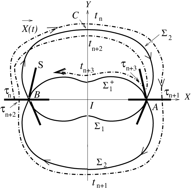
The amplitude of the rate of change of the time interval $d(t_{n+1}-t_{n})/dt_{n}$ can then be calculated from equations (21) and (21):

By writing that this quantity is equal to unity on the border of the stochastic layer (Rom-Kedar [15]) we obtain the energy $H_{s}$ corresponding to this boundary:

The boundary of the stochastic layer around $\Sigma_{2}$ can then be obtained by setting $i=2$ in the above formula. The curve $\psi_{r0}=H_{s}$ has been plotted on the numerical Poincaré sections of Fig. 4 for comparison (thick black line), and we observe that, in spite of the rough approximations of the model, this curve corresponds to the border of the stochastic zone with an acceptable accuracy.

Result (25) can also be used to determine the distance $r_{C}$ between the border of the stochastic layer and point $C$, which can be thought of as the half-thickness of the stochastic layer at $C$. Indeed, by writing that $\psi_{r0}(\vec{X}_{C}+r_{C}\vec{e}_{Y})=H_{s}$, and using a first-order Taylor expansion (assuming that $r_{C}$ is small):

where $\gamma=\partial\psi_{r0}/\partial Y(C)\simeq 1.67$. The thickness of the stochastic layer of $\Sigma_{2}$ at $C$ is therefore: $\Delta_{C}=2r_{C}\simeq 15.8\epsilon^{2}.$ This formula is compared to measurements of the thickness $\Delta_{C}$ obtained from numerical computations (Fig. 6). Three kinds of computations are used here: Poincaré sections, particle clouds computed by using the asymptotic velocity in the rotating frame, and particle clouds computed by using the exact potential velocity (1) in the laboratory frame. Point $C$ has been chosen for these measurements because the thickness is well-defined there. We observe that the order-of-magnitude of $\Delta_{C}$ is well predicted by the theory, especially if $\varepsilon$ is small. For larger $\varepsilon$ discrepancies of about 100% appear, and these errors are known to be due to resonances occurring in the fluid point dynamics (Luo & Han [19], Trueba & Baltanas [17]) and to regular islands embedded in the stochastic layer. In spite of these discrepancies we can conclude that the theoretical prediction obtained from the separatrix map gives an acceptable lower bound to the thickness of the stochastic zone.

The typical size of the stochastic layer can also be estimated in the vicinity of the hyperbolic points $A$ (and $B$) , by writing that $\psi_{r0}(\vec{X}_{A}+r_{A}\vec{e}_{X})=H_{s}$, where $r_{A}$ is the distance from $A$ to the external border of the stochastic zone, towards $\vec{e}_{X}$. To obtain $r_{A}$ we then use a second-order Taylor expansion (assuming that $r_{A}$ is small). Indeed, because $A$ is a stagnation point of the unperturbed flow, the gradient of $\psi_{r0}$ vanished there, and we are left with:

The typical size of the stochastic layer is therefore larger in the vicinity of $A$ (and $B$) than anywhere else, in the limit where $\varepsilon$ is small. This is a rather general result which is a consequence of the fact that $A$ and $B$ are stagnation points [16]. Here also we expect (27) to provide only a lower bound of the actual $r_{A}$, since resonances might occur and make the thickness even bigger.

The asymptotic model presented in the above sections shows that some chaotic mixing must occur in the vicinity of a vortex pair as soon as a wall is present in the surroundings of the two vortices. In order to check the reliability of these calculations, which are valid only if the wall is far from the vortices, we have performed some calculations of fluid points transport by using the exact potential velocity field (1) (set dimensionless by using $\Omega_{0}$ and $d_{0}$), in the laboratory frame.

Fig. 7 shows two particle clouds corresponding to $L_{0}=10d_{0}$ and $5d_{0}$ (that is $\varepsilon=0.1$ and $0.2$, respectively). Because our goal is to visualize fluid point mixing in the stochastic zone, the initial cloud is taken to be a small spot of size $0.1\times 0.1$ centered at $I$ (which is initially located at $(0,0)$). The initial positions of the vortices are $(x_{1},y_{1})=(1+\varepsilon^{2}/2,1/\varepsilon)$ and $(x_{2},y_{2})=(-1-\varepsilon^{2}/2,1/\varepsilon)$. The final time of the three simulations is $t=50\pi$, and the final location of the centre point is very close to the asymptotic value $(x_{I},y_{I})\approx(2\varepsilon\,t,L_{0})$ in both cases. We observe that some particles collect on a structure which is very close to the separatrices $\Sigma_{i}$ described above, as a consequence of the existence of a stochastic zone in the vicinity of these separatrices. The thickness of the stochastic zone is of the order of the theoretical one, as shown in Fig. 6 (filled circles).

As noticed above, $L_{0}$ and $\Gamma$ being the relevant scales of the external flow, we non-dimensionalize the streamfunction (1) by using $L_{0}$ for lengths and $\Gamma/4\pi L_{0}$ for velocities. Also, we consider the reference frame translating at the velocity $\dot{x}_{I}^{0}={\Gamma}/{2\pi L_{0}}$ of a vortex with strength $2\Gamma$, placed at distance $L_{0}$ from the wall. The non-dimensional streamfunction of the flow induced by the four vortices with strengths $\Gamma,\Gamma,-\Gamma,-\Gamma$, in this frame, is:

where $\psi(x,y,t)$ is the streamfunction of the flow observed in the laboratory frame, and stars indicate non-dimensional variables. Still assuming that $\varepsilon=d_{0}/L_{0}\ll 1$, and using Eqs. (12) and (13) for the vortex motion, the streamfunction can be expanded as:

where $\psi_{0*}(x_{*},y_{*})=2\log[(x_{*}^{2}+y_{*}^{2}+1+2y_{*})/(x_{*}^{2}+y_{*}^{2}+1-2y_{*})]-2y_{*}$ is the streamfunction of a simple dipole centered at (0,0) (i.e. single vortex plus its mirror vortex, see Fig. 8(b)), and the $\varepsilon^{2}$ terms manifest the fact that we have a vortex pair with strength $\Gamma+\Gamma$, instead of a single vortex with strength $2\Gamma$, so that the flow is unsteady. The streamfunctions $\psi_{2c}$ and $\psi_{2s}$ are steady, rational functions of $x_{*}$ and $y_{*}$ only.

With the time scale used here, the rotation of the vortex pair is fast, so that the flow (29) is a rapidly perturbed dipolar flow. Fig. 8(a) shows this streamfunction when $\varepsilon=0.3$ (dashed line), together with the exact four-vortex streamfunction already discussed (solid line). The two flows are very close, except in the vicinity of both pairs, as expected. The $O(\varepsilon^{3})$ terms in (29) are identically zero (for symmetry reasons), and this is why the agreement is good even if $\varepsilon$ is not very small here. For $\varepsilon\leq 0.2$ dashed lines and solid lines (not shown here) are indistinguishable, except in the very vicinity of the vortices.

Particle motion can therefore be approximated by a perturbed hamiltonian system, with hamiltonian $\psi_{0*}$. The Melnikov function attached to the cycle $S_{1}S_{2}$ reads (removing the stars):

where $\vec{q}(t)$ runs on the unperturbed cycle, and is chosen such that $\vec{q}(0)$ coincides with point C of Fig. 8(b). This Melnikov function approximates (to order $\varepsilon^{2}$) the "energy" difference $\psi_{0}(\vec{X}(\tau_{2}))-\psi_{0}(\vec{X}(\tau_{1}))$, where $\vec{X}(t)$ is the trajectory of a fluid point advected by the perturbed flow, with a trajectory very close the separatrix $S_{1}S_{2}$. The times $\tau_{1}$ and $\tau_{2}$ correspond to the particle passing near the saddle points $S_{1}$ and $S_{2}$. Because our perturbation is rapid, the amplitude of the Melnikov function will now depend on $\varepsilon$ (Gelfreich [20]). The integrands in the above integrals are unknown analytically, they are however localized around zero and decay exponentially. We have chosen to approximate them with a mixed polynomial/gaussian expression of the form $P(t)/\cosh^{2}(\delta\,t)$, where $P$ is a fitted polynomial and $\delta$ is a fitted constant. The integrals can then be obtained analytically, and we are led to $M_{ext}(t_{0})=A(\varepsilon)\sin({2t_{0}}/{\varepsilon^{2}})$, with:

where $\delta$ and $\gamma$ are purely numerical constants depending on the fitting procedure: $\gamma\approx 18$, $\delta\approx 5$. Note that this formula depends on the form chosen to approximate our integrands. This is therefore a numerical result, rather than a truely analytical one, being understood that other fittings might not significantly affect the numerical values of the amplitude of the Melnikov function. Because $A(\varepsilon)>0$ for all $\varepsilon$, and $M_{ext}(t_{0})$ always has simple zeros when $t_{0}$ varies, portions of fluid will be exchanged between the interior of the cycle $S_{1}S_{2}$, and the fluid outside. However, the amplitude is so small as soon as $\varepsilon\leq 0.2$ (i.e. $A(0.2)<7\,10^{-5}$), that mixing through the cycle $S_{1}S_{2}$ should be hardly visible for such small $\varepsilon$’s. In contrast, when $\varepsilon$ increases above 0.2, $A(\varepsilon)$ quickly reaches values of order unity. By constructing the separatrix map of $S_{1}S_{2}$, one can derive the theoretical thickness $\Delta$ of the stochastic layer surrounding the outer homoclinic cycle. In the vicinity of point C of Fig. 8(b), we are led to $\Delta_{C}\approx 0.5A(\varepsilon)$. This quantity has been plotted in Fig. 6 (dashed line). We indeed observe that the thickness is exponentially small when $\varepsilon\leq 0.2$ ($L_{0}\geq 5d_{0}$), and quickly reaches values of order unity as soon as $\varepsilon$ is larger than about 0.25. [Note that, even though the diagram suggests a sharp increase of $\Delta_{C}$, there is no critical $\varepsilon$ here: the Melnikov function has simple zeros for all $\varepsilon$.] Fig. 6 suggests that the vortex pair might be apparently separated from the outer open flow when $L_{0}\geq 5d_{0}$, since the whole vortex system will be surrounded by an extremely thin stochastic zone. Also, the thickness of this stochastic zone should quickly reach a value of order unity as soon as $L_{0}\leq 3d_{0}$. These two points are checked numerically in the next paragraph.

Computations of particle clouds in the laboratory frame, using the exact four-vortex potential solution (1), have been performed. Particles have been injected at $t=0$ near the vortices (in box A of Fig. 8(b)). Also, to check whether portions of fluid could enter within the cycle $S_{1}S_{2}$, we have injected another set of particles outside the cycle $S_{1}S_{2}$ (in box B of Fig. 8(b)). These simulations confirm the significant difference between the thickness of the inner cycle and the one of the outer cycle, as suggested by the theoretical curves of Fig. 6.

Indeed, Fig. 9(a) shows the two particle clouds at $t=100\pi$, when $L_{0}/d_{0}=5$ ($\varepsilon=0.2$). Units are the same as in the simulations of section III, that is: $d_{0}$ for lengths and $\Omega_{0}$ for times. Particles marked with black dots are those which have been injected in box A (they are also indicated with a (A)), and those marked with empty circles have been injected in box B (they are also indicated with a (B)). Even though these computations have been conducted in the laboratory frame, the homoclinic cycles appearing in the rotating frame (section III) and in the translating frame (section IV.1), naturaly appear here. Particles injected near vortices wander in the vicinity of the inner cycle $\Sigma_{2}\cup\Sigma_{1}$ investigated in section III, whereas those injected ahead of the vortices move in the vicinity of the outer cycle $S_{1}S_{2}$. Some particles penetrate within this cycle, in agreement with the fact that the Melnikov function has simple zeros. When $L_{0}/d_{0}=4$ (Fig. 9(b)) the thickness of the inner stochastic zone around the cycle $\Sigma_{2}$ is larger, whereas the thickness of the outer stochastic zone around the cycle $S_{1}S_{2}$ does not appear to be very different from case (a), in agreement with the theoretical thickness calculated in the previous section (dashed line of Fig. 6). When $L_{0}/d_{0}=3.5$ (Fig. 9(c)) the thickness of the outer stochastic zone is slightly larger than in case (b), but the two clouds are still separated. For $L_{0}/d_{0}=3.2$ ($\varepsilon=0.3125$, Fig. 9(d)) the two particle clouds mix significantly, in agreement with the fact that the amplitude of the Melnikov function is of order unity there. However, the thickness of the outer stochastic zone cannot be measured from these graphs and compared to the theoretical value of $\Delta_{C}$: this is due to the fact that particles injected in box B now mix with those injected in box A. These simulations confirm, however, that the outer stochastic zone remains negligible compared to the inner one as long as $L_{0}/d_{0}$ is larger than about 4, so that the vortex pair might exchange very little fluid with the outer flow in this case.

References

- [1] P. FLOHR and J.C. VASSILICOS. Accelerated scalar dissipation in a vortex. J. Fluid Mech., 348:295–317, 1997.
- [2] K. BAJER. Flux expulsion by a point vortex. European Journal of Mechanics - B/Fluids, 17(4):653–664, 1998.
- [3] H. AREF. Stirring by chaotic advection. J. Fluid Mech., 143:1–21, 1984.
- [4] H. AREF. The development of chaotic advection. Phys. Fluids, 14(4):1315–1325, 2002.
- [5] D. BEIGIE, A. LEONARD, and S. WIGGINS. Invariant manifold templates for chaotic advection. Chaos, Solitons & Fractals, 4(6):749–868, 1994.
- [6] A. WONHAS and VASSILICOS. Mixing in frozen and time-periodic two-dimensional vortical flows. J. Fluid Mech., 442:359–385, 2001.
- [7] A. PENTEK, T. TEL, and Z. TOROCZKAI. Chaotic advection in the velocity field of leapfrogging vortex pairs. J. Phys. A: Math. Gen., 28:2191–2216, 1995.
- [8] V. ROM-KEDAR, A. LEONARD, and S. WIGGINS. An analytical study of transport, mixing and chaos in an unsteady vortical flow. J. Fluid Mech., 214:347–394, 1990.
- [9] D.J. ACHESON. Instability of vortex leapfrogging. Eur. J. Phys., 21:269–273, 2000.
- [10] X. CARTON, G. MAZE, and B. LEGRAS. A two-dimensional vortex merger in an external strain field. Journal of Turbulence, 3:045, 2002.
- [11] G. MAZE, X. CARTON, and G. LAPEYRE. Dynamics of a 2D vortex doublet under external deformation. Regular and Chaotic Dynamics, 9(4):477–497, 2004.
- [12] J. R. ANGILELLA. Dust trapping in vortex pairs. Physica D: Nonlinear Phenomena, 239:1789–1797, 2010.
- [13] B.V. CHIRIKOV. A universal instability of many-dimensional oscillator systems. Physics Reports, 52(5):263–379, 1979.
- [14] J.B. WEISS and E. KNOBLOCH. Mass transport and mixing by modulated travelling waves. Physical Review A, 40(5):2579–2589, 1989.
- [15] V. ROM-KEDAR. Homoclinic tangles - classification and applications. Nonlinearity, 7:441–473, 1994.
- [16] L. KUZNETSOV and G. M. ZASLAVSKY. Regular and chaotic advection in the flow field of a three-vortex system. Phys. Rev. E, 58(6):7330–7349, 1998.
- [17] J.L. TRUEBA and J.P. BALTANAS. On the estimate of the stochastic layer width for a model of tracers dynamics. Chaos, 13(3):866–873, 2003.
- [18] S. BALASURIYA. Optimal perturbation for enhanced chaotic transport. Physica D, 202:155–176, 2005.
- [19] A. C. J. LUO and A.P.S. HAN. The resonance theory for stochastic layers in nonlinear dynamic systems. Chaos, Solitons and Fractals, 12:2493–2508, 2001.
- [20] V. G. GELFREICH. Melnikov method and exponentially small splitting of separatrices. Physica D., 101:227–248, 1997.