Stabilizing the spiral order with spin-orbit coupling in an anisotropic triangular antiferromagnet

Antiferromagnets on the triangular lattice represent a prototype correlated systems where certain novel mangetic phases such as the spin liquid state may emerge due to the quantum fluctuations and geometric frustrations[1]. Some materials candidates of the spin liquid, such as the organic $\kappa-(BEDT-TTF)_{2}Cu_{2}(CN)_{3}$[2] and $EtMe_{3}Sb[Pd(dmit)_{2}]_{2}$[3], are the triangular-lattice antiferromagnets, where the interchain coupling $J^{\prime}$ is close to the intrachain coupling $J$. Another layered quantum magnet, $Cs_{2}CuCl_{4}$[4], has a relatively large spatial anisotropy $\alpha\equiv J^{\prime}/J\sim 0.34$. The inelastic neutron scattering measurements reveal the possible spin liquid phase for temperature above $T_{N}=0.62K$, while for $T<T_{N}$, the spiral order is set up[5]. The emergent spiral order is attributed to the interlayer coupling and the small Dzyaloshinskii-Moriya (DM) interaction[6, 7, 8, 9] which is put by hand in the Heisenberg model. On the other hand, the SOC is ubiquitous in materials whose crystal structures lack the inversion symmetry, and $Cs_{2}CuCl_{4}$ just falls into this category.

Theoretically, though the SOC has been extensively studied for the electronic systems with relatively small Coulomb interaction $U$, it remains challenging to understand the effect of SOC when $U$ is moderate or strong. In this paper, we study the Hubbard model on anisotropic triangular lattice with the finite SOC and the infinite $U$. The spatial anisotropy $\alpha$ in the studied model is an important tuning parameter which interpolates the decoupled chains ($\alpha\rightarrow 0$) and the square lattice ($\alpha\rightarrow\infty$). In the absence of the SOC, a quasi one-dimensional spin liquid phase and a two-dimensional magnetic phase emerge at the half-filling in the two limiting cases, respectively. Thus by increasing $\alpha$, it is natural to expect a critical $\alpha_{c}$, separating the spin liquid and magnetic ordered states. Various numerical calculations for finite clusters [10, 11, 12] obtain $\alpha_{c}\sim 0.7-0.9$, while the linear spin-wave theory[13] predicts a much smaller value $\alpha_{c}=0.27$. Here we shall mainly focus on the magnetic ordered phase and study the influence of the SOC by using the Schwinger-boson mean-field theory.

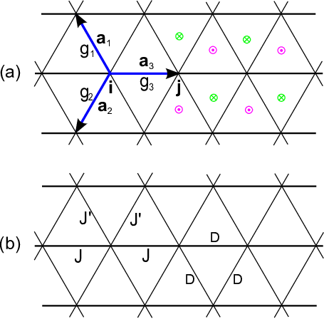
Our starting point Hamiltonian is the Hubbard model on triangular lattice with the SOC, defined by

Where, $t_{\mathbf{i}\mathbf{j}}$ is the hopping energy between the nearest neighboring bond $\langle\mathbf{i}\mathbf{j}\rangle$, $c_{\mathbf{i}\sigma}$ annihilates an electron at $\mathbf{i}$ with the spin index $\sigma=+/-$ for up/down spins, $g_{\mathbf{i}\mathbf{j}}$ represents the strength of the SOC. We shall at first drive an equivalent spin model with finite SOC for large U and at half-filling. This has been recently realized for the same model defined on the kagome lattice[14]. Here the similar approach is illustrated by the two-site problem. Noticed that the bond $\langle\mathbf{i}\mathbf{j}\rangle$ is oriented, the SOC brings an stagger flux through each triangle plaquette as shown in Fig.1(a). Thus the first term can be re-expressed by $-\tilde{t}_{12}\sum_{\sigma}(e^{-i\sigma D_{12}}c_{1\sigma}^{{\dagger}}c_{2\sigma}+h.c.)$, with $\tilde{t}_{12}=\sqrt{t_{12}^{2}+g_{12}^{2}}$ and $D_{12}=\arctan{(g_{12}/t_{12})}$. By performing the site and spin-dependent $U(1)$ transformation: $\tilde{c}_{1\sigma}=e^{i\sigma(D_{12}/2)}c_{1\sigma}$, $\tilde{c}_{2\sigma}=e^{-i\sigma(D_{12}/2)}c_{2\sigma}$, the corresponding Hamiltonian (at the large U limit) is mapped to the spin Hamiltonian $J_{12}\bf{\tilde{S}_{1}}\cdot\bf{\tilde{S}_{2}}$ with $J_{12}=\frac{4\tilde{t}_{12}^{2}}{U}$ and $\mathbf{\tilde{S}_{i}}=\frac{1}{2}\sum_{\sigma\sigma^{\prime}}\tilde{c}^{{\dagger}}_{i\sigma}\vec{\sigma}_{\sigma\sigma^{\prime}}\tilde{c}_{i\sigma^{\prime}}$.

Noticed that the triangular lattice is not a bipartite lattice, there exists no compatible $U(1)$ transformation for every site. For a lattice model, we should transform back to the original fermion operators. Therefore, the spin model for the strong-coupled Hubbard model on the half-filled triangular lattice turns out to be

where $S^{\pm}=S^{x}\pm iS^{y}$. The SU(2) symmetry of the above spin model is broken by the SOC. And its antisymmetric (the DM-term ) and symmetric parts appear with explicit SOC-dependent coupling strengths.

We then study the Hamiltonian (2) using the Schwinger-boson mean-field theory[15]. The spin operators are represented by boson operators $S^{+}=b^{{\dagger}}_{\uparrow}b_{\downarrow}$, $S^{-}=b^{{\dagger}}_{\downarrow}b_{\uparrow}$, $S^{z}=\frac{1}{2}(b^{{\dagger}}_{\uparrow}b_{\uparrow}-b^{{\dagger}}_{\downarrow}b_{\downarrow})$, with the constraint $b^{{\dagger}}_{\uparrow}b_{\uparrow}+b^{{\dagger}}_{\downarrow}b_{\downarrow}=1$. We introduce the mean-fields $\psi_{n\sigma}=-i\sigma\langle b_{\mathbf{i}\sigma}b_{\mathbf{i}+\mathbf{a}_{n}\bar{\sigma}}\rangle$, with $\mathbf{a}_{1}=a_{0}(-\frac{1}{2},\frac{\sqrt{3}}{2})$, $\mathbf{a}_{2}=a_{0}(-\frac{1}{2},-\frac{\sqrt{3}}{2})$, $\mathbf{a}_{3}=-(\mathbf{a}_{1}+\mathbf{a}_{2})=a_{0}(1,0)$, and $a_{0}$ is the lattice constant, as marked in Fig.1(a). The obtained mean-field Hamiltonian is

where the $\lambda$-term is introduced to impose the constraint.

In the momentum space, the Hamiltonian has the form

where $N=N_{1}\times N_{2}$ is the site number of the lattice ( $\mathbf{a}_{1}$ and $\mathbf{a}_{2}$ are chosen as the two primitive translation vectors), $A_{\mathbf{k}}=\frac{i}{2}\sum_{n\sigma}\bar{\sigma}J_{n}(\psi_{n\sigma}+e^{2i\bar{\sigma}D_{n}}\psi_{n\bar{\sigma}})e^{i\sigma\mathbf{k}\cdot\mathbf{a}_{n}}$. We assume that $A_{\mathbf{k}}$ is a real number, because the phase factor of $A_{\mathbf{k}}$ can be gauged away by the U(1) transformation. Due to the time-reversal symmetry, we also have $|\psi_{n\uparrow}|=|\psi_{n\downarrow}|$. Thus we use the ansatz $\psi_{n\sigma}=\psi_{n}e^{i\sigma\vartheta_{n}}$, and obtain $A_{\mathbf{k}}=2\sum_{n}J_{n}\sin{(\mathbf{k}\cdot\mathbf{a}_{n}-D_{n})\cos{(D_{n}+\vartheta_{n})}}\psi_{n}$.

The mean-field Hamiltonian Eq.(4) is diagonalized by the bosonic Bogliulov transformation, $b_{\mathbf{k}\uparrow}=u_{\mathbf{k}}\alpha_{\mathbf{k}\uparrow}+v_{\mathbf{k}}\alpha_{\mathbf{k}\downarrow}^{{\dagger}}$, $b_{-\mathbf{k}\downarrow}=u_{\mathbf{k}}\alpha_{\mathbf{k}\downarrow}+v_{\mathbf{k}}\alpha_{\mathbf{k}\uparrow}^{{\dagger}}$, with $u_{\mathbf{k}}^{2}=\frac{\lambda}{2\omega_{\mathbf{k}}}+\frac{1}{2}$, $v_{\mathbf{k}}^{2}=\frac{\lambda}{2\omega_{\mathbf{k}}}-\frac{1}{2}$, and $u_{\mathbf{k}}v_{\mathbf{k}}=-\frac{A_{\mathbf{k}}}{2\omega_{\mathbf{k}}}$. Then

where the quasiparticle dispersion $\omega_{\mathbf{k}}=\sqrt{\lambda^{2}-A_{\mathbf{k}}^{2}}$. A stable ground state requires $\lambda\geq|A_{\mathbf{k}}|$. The free energy is given by

with $\beta=\frac{1}{k_{B}T}$. The Lagrangian multiplier $\lambda$ is determined by optimizing the free energy, leading to

where $n_{b}(\omega_{\mathbf{k}})=\frac{1}{e^{\beta\omega_{\mathbf{k}}}-1}$ is the Bose distribution function. The mean-fields $\psi_{n}$ and $\vartheta_{n}$ are then calculated self-consistently through following equations,

Keeping in mind that $J_{n}=(t_{n}^{2}+g_{n}^{2})/U$ and $D_{n}=\arctan{(g_{n}/t_{n})}$, we set $J_{1}=J_{2}=J^{\prime}$, $J_{3}=J$, and $D_{1}=D_{2}=D_{3}=D$ as illustrated in Fig.1(b). Thus the spatial anisotropy is measured by $\alpha\equiv J^{\prime}/J$. Three special cases in the parameter space are $(1)$ $\alpha=0$, the decoupled chain’s limit; $(2)$ $\alpha=\infty$, the square lattice limit; and $(3)$ $\alpha=1$, the isotropic point. Notice that with this choice of parameters, the mean-field equations are invariant under the exchange of the bond index $1$ and $2$. Therefore, we have $\psi_{1}=\psi_{2}$ and $\vartheta_{1}=\vartheta_{2}$.

According to the analysis with functional integral method[16], no bosons can condense in the two-dimensional lattices at finite temperature. This is consistent with the Mermin-Wagner theorem[17]. In the case of a gapped energy spectrum, i.e. $\min{\omega(\mathbf{k})}\neq 0$, there is no Bose-Einstein condensation and the ground state is a spin liquid. Otherwise, if the spectrum is gapless, the bosons can condense on the lowest energy state, implying a long-range magnetic order.[18] The relation between magnetic order and Bose-Einstein condensation can be drawn from the spin-spin correlation whose diagonal components are given by

where,

It is important to recall that when $D=0$, i.e., in the absence of the SOC, $A_{-\mathbf{k}}=-A_{\mathbf{k}}$, the SU(2) symmetry is restored. Then there always exists a pair of zero modes of $\omega(\mathbf{k})$ with $\mathbf{k}=\pm\mathbf{k}^{*}$, condensed at zero temperature. However, for non-zero SOC, $D\neq 0$, we find that $A_{-\mathbf{k}}\neq-A_{\mathbf{k}}$ in general and $\omega(\mathbf{k})$ has only a single zero mode $\mathbf{k}^{*}$ in the first Brillouin zone, so the expression for $x-$ or $y-$component of the spin-spin correlation is different from that of the z-component. According to Eq. (10), the spin-spin correlation between the $z$-components vanishes at zero temperature when the distance between two spins is sufficiently large. Moreover, there exits one independent nonvanishing off-diagonal component, $\langle S^{y}_{\mathbf{0}}S^{x}_{\mathbf{i}}\rangle=-\langle S^{x}_{\mathbf{0}}S^{y}_{\mathbf{i}}\rangle=\frac{1}{2}Im(f_{\mathbf{i}}^{2}+g_{\mathbf{i}}^{2})$. All these features are in contrast with the cases studied previously[19, 18, 16].

Now we discuss the numerical results for the infinite system. By converting the sum in the mean-field equations (11) and (12) into integrals and denoting the contribution from the Bose condensate as $b_{0}$, the mean-field equations for numerical performance are

where $B_{0}=\frac{1}{\lambda}A_{\mathbf{k^{*}}}e^{-i\mathbf{k}^{*}\cdot\mathbf{a}_{n}}b_{0}$ if $b_{0}>0$, and $B_{0}=0$ if $b_{0}<0$. To have a gapless spectrum, $\lambda$ is always fixed at the largest value of $|A_{\mathbf{k}}|$. If the solution is associated with a negative $b_{0}$, we can always fulfill the constraint (11) by tuning up $\lambda$ slightly. In this case, the energy spectrum is gapped and the system is in the spin liquid phase. If there is a solution with a positive $b_{0}$, then the system is in the condensation phase. The magnetic order can be obtained from the spin-spin correlation functions. They are $\langle S^{x}_{\mathbf{0}}S^{x}_{\mathbf{i}}\rangle=\langle S^{y}_{\mathbf{0}}S^{y}_{\mathbf{i}}\rangle=b_{0}^{2}\cos{(2\mathbf{k}^{*}\cdot\mathbf{i})}$ and $\langle S^{y}_{\mathbf{0}}S^{x}_{\mathbf{i}}\rangle=-\langle S^{x}_{\mathbf{0}}S^{y}_{\mathbf{i}}\rangle=b_{0}^{2}\sin{(2\mathbf{k}^{*}\cdot\mathbf{i})}$. By denoting $\mathbf{k}^{*}=(k_{1}^{*},k_{2}^{*})$, we have the ordering wave vectors, along the directions of $\mathbf{a}_{1}$, $\mathbf{a}_{2}$ and $\mathbf{a}_{3}$, being $2k_{1}^{*}$, $2k_{2}^{*}$ and $-2(k_{1}^{*}+k_{2}^{*})$, modulo-divided by $2\pi$, respectively.

The numerical solutions for $\mathbf{k}^{*}$ show that $k_{1}^{*}=k_{2}^{*}=k^{*}$. The curves of $k^{*}$ as a function of $\alpha\equiv J^{\prime}/J$ are plotted in Fig.2. When $D$ is very small, the ordering wave vector along the chain tends to $\pi$ near the decoupled-chain limit ($\alpha\ll 1$), indicating an antiferromagnetic order. While when $\alpha\gg 1$, the ordering wave vectors along the directions of $\mathbf{a}_{1}$, $\mathbf{a}_{2}$ tend to $\pi$, $\pi$, respectively, reproducing the checkerboard or Neel ordering for the unfrustrated antiferromagnet in a square lattice. Between the two limits the spiral order develops and the order parameter oscillates with the distance. With the increase of $D$, the curves of $k^{*}$ change dramatically. Especially, when $D=\frac{1}{6}\pi$, $k^{*}=\frac{2}{3}\pi$ is independent of $\alpha$. For generic $D$, the limiting values of $k^{*}$ with small and large $\alpha$ are $\frac{3}{4}\pi-\frac{1}{2}D$ and $\frac{1}{2}\pi+D$ respectively. It is also interesting to note that at the isotropic point ($\alpha=1$), $k^{*}$ always equals to $\frac{2}{3}\pi$ regardless of $D$.

The square-root of the amplitude of the spin-spin correlation function, characterizing the strength of the magnetic order, is exactly the Bose condensation density $b_{0}$. In the case of the antiferromagnetic order, $b_{0}$ is equal to the sublattice magnetization. It is also a function of $D$ with period $\pi/3$ since the SOC can be related to the phase factor in the triangular lattice. As shown in Fig 3, $b_{0}$ is enhanced monotonically when $D$ increases up to $\pi/6$. For each $D$, $b_{0}$ takes a maximum value at $\alpha=1$.

For each fixed $D$ there is a critical value $\alpha_{c}\equiv J^{\prime}_{c}/J$ separating the spin liquid phase from the magnetic ordered phase. For $\alpha<\alpha_{c}$, $b_{0}=0$ and all the spin-spin correlation functions decay exponentially to zero as the distance $\mathbf{i}\rightarrow\infty$. For $\alpha>\alpha_{c}$, the bosons condense on the state with momentum $\mathbf{k}^{*}$. Fig. 4 plots the critical line of the quantum phase transition. As a function of $D$, the critical line oscillates with period $\pi/3$ as expected. In realistic materials, the strength of the SOC is usually small compared to the hopping integral and the large $D$ in the phase diagram is unphysical. However, large value of D is achievable in the optical flux lattice[20]. We find that the nonzero $D$ (within the half-period $\pi/6$) pushes the boundary to the region with a smaller $\alpha$, thus it effectively enhances the magnetic ordering. This feature is compatible with the $D$-dependence of $b_{0}$. When $D=\frac{\pi}{6}$, $\alpha_{c}$ reaches the minimum value $0.095$. This result implies that with relatively large SOC the spiral magnetic order can emerge in the triangular lattice which has a tendency of reducing dimensionality as featured by small $\alpha$.

Finally, we remark that our mean-field treatment emphasizes the magnetic ordering but is not adequate to capture the disordered state which may appear in the region with the moderate spatial anisotropy. Focusing on the spiral ordered phase with small anisotropy, it is possible that the quantum fluctuations could blur the difference between the solutions with two condensation momenta and a single momentum, giving rise to a finite spin-spin correlation between $z$-components. While this issue can be clarified in the future by taking into account the quantum fluctuations above the mean-field solution, it is robust that the SOC induces a nonzero spin correlation between the $x$- and $y$-components, suppresses the spin correlation between the $z$-components and favors the establishment of the spiral order.

In summary, a large-U Hubbard model with the SOC on an spatial anisotropic lattice at half-filling is studied using the Schwinger- boson method. With the participation of the SOC, the condensation momentum of the Schwinger bosons have only a single zero mode which in turn leads to a finite spin-spin correlation between $x$- and $y$-components and a vanishing spin-spin correlation between $z$-components at large distance. The SOC also shifts the phase boundary between the magnetic ordered state and the spin liquid state to the larger anisotropy side, and stabilizes the spiral magnetic order. Our results provide an alternative understanding of the spiral order observed in some materials like $Cs_{2}CuCl_{4}$ where the triangular lattice has a relatively small $\alpha$.

This work was supported in part by the NSFC, the NSF of Zhejiang Province, and the 973 Project of the MOST.

References

- [1] P.W. Anderson, Mater. Res. Bull. 8, 153(1973); P. Fazekas and P. Anderson, Philos. Mag. 30, 432(1974).
- [2] Y. Shimizu, K. Miyagawa, K. Kanoda, M. Maesato, and G. Saito, Phys. Rev. Lett. 91, 107001(2003).
- [3] T. Itou, A. Oyamada, S. Maegawa, M. Tamura, and R. Kato, Phys. Rev. B 77, 104413(2008).
- [4] R. Coldea, D.A. Tennant, K. Habicht, P. Smeibidl, C. Wolters, and Z. Tylczynski, Phys. Rev. Lett. 88, 137203(2002).
- [5] R. Coldea, D. A. Tennant, and Z. Tylczynski, Phys. Rev. B 68, 134424(2003).
- [6] I. Dzyaloshinkii, J. Phys. Chem. Solids 4, 241(1958); T. Moriya, Phys. Rev. 120, 91(1960).
- [7] S. Ghamari, C. Kallin, S.-S. Lee, E.S. Srensen, arXiv:1108.3036(2011).
- [8] D. Dalidovich, R. Sknepnek, A.J. Berlinsky, J. Zhang, and C. Kallin, Phys. Rev. B 73, 184403(2006).
- [9] J.O. Fjrestad, Weihong Zheng, R.R.P. Singh, R.H. McKenzie, and R. Coldea, Phys. Rev. B 75, 174447(2007).
- [10] M.Q. Weng, D.N. Sheng, Z.Y. Weng, and R.J. Bursill, Phys. Rev. B 74, 012407(2006).
- [11] D. Heidarian, S. Sorella, and F. Becca, Phys. Rev. B 80, 012404(2009).
- [12] J. Reuther and R. Thomale, Phys. Rev. B 83, 024402(2011).
- [13] A.E. Trumpe, Phys. Rev. B 60, 2987(1999).
- [14] J.W. Mei, E. Tang, and X.G. Wen , arXiv:1102.2406(2011).
- [15] A. Auerbach, Interacting Electrons and Quantum Magnetism (Springer-Verlag, New York, 1994).
- [16] A. Auerbach and D.P. Arovas, Phys. Rev. Lett. 61, 617(1988).
- [17] N.D. Mermin and H. Wagner, Phys. Rev. Lett. 17, 1133(1966).
- [18] S.Q. Shen and F.C. Zhang, Phys. Rev. B 66, 172407(2002).
- [19] S. Sanker, C. Jayaprakash, H.R. Krishnamurthy, and M. Ma, Phys. Rev. B 40, 5028(1989).
- [20] N.R. Cooper, Phys. Rev. Lett. 106, 175301(2011).