跳到论文正文
W Papers独立论文阅读器 arXiv:1109.2005 论文正文 计算阅读时间 · 0%
引用这篇论文根据当前论文元数据生成,正式投稿前建议核对。


License: arXiv.org perpetual non-exclusive license
arXiv:1109.2005v1 [math.NA] 09 Sep 2011

Convergent Numerical Schemes for the Compressible Hyperelastic Rod Wave Equation

David Cohen Raynaud
Center of Mathematics for Applications
University of Oslo
NO–03160316 Oslo
Norway
Email address: xavierra@cma.uio.no URL: http://folk.uio.no/xavierra/
and Xavier Raynaud Cohen
Mathematisches Institut
Universität Basel
CH–40514051 Basel
Switzerland
Email address: david.cohen@unibas.ch URL: http://www.math.unibas.ch/˜cohen/
Date: August 24, 2026
Abstract.

We propose a fully discretised numerical scheme for the hyperelastic rod wave equation on the line. The convergence of the method is established. Moreover, the scheme can handle the blow-up of the derivative which naturally occurs for this equation. By using a time splitting integrator which preserves the invariants of the problem, we can also show that the scheme preserves the positivity of the energy density.

Key words and phrases: 
Hyperelastic rod wave equation, Camassa–Holm equation, numerical scheme, positivity, invariants
2000 Mathematics Subject Classification
Primary: 65M06, 65M12; Secondary: 35B99, 35Q53

1. Introduction

We consider the compressible hyperelastic rod wave equation

ut−ux​x​t+3​u​ux−γ⁡(2​ux​ux​x+u​ux​x​x)=0.u_{t}-u_{xxt}+3uu_{x}-\gamma(2u_{x}u_{xx}+uu_{xxx})=0. (1)

The equation is obtained by Dai in [6] as a model equation for an infinitely long rod composed of a general compressible hyperelastic material. The author considers a far-field, finite length, finite amplitude approximation for a material where the first order dispersive terms vanish. The function u=u⁡(t,x)u=u(t,x) represents the radial stretch relative to a prestressed state. The parameter γ∈ℝ\gamma\in\mathbb{R} is a constant which depends on the material and the prestress of the rod and physical values lie between -29.4760 and 3.4174. For materials where first order dispersive terms cannot be neglected, the KdV equation

ut+u​ux+ux​x​x=0u_{t}+uu_{x}+u_{xxx}=0

applies and only smooth solitary waves exists. In contrast, the hyperelastic rod equation (1) admits sharp crested solitary waves.

The Cauchy problems of the hyperelastic rod wave equation on the line and on the circle are studied in [5] and [15], respectively. The stability of a class of solitary waves for the rod equation on the line is investigated in [5]. In [12], Lenells provides a classification of all traveling waves. In [5, 15], the authors establish, for a special class of initial data, the global existence in time of strong solutions. However, in the same papers, they also present conditions on the initial data for which the solutions blow up and, in that case, global classical solutions no longer exist. The way the solution blows up is known: In the case γ>0\gamma>0, there is a point x∈ℝx\in\mathbb{R} and a blow-up time TT for which limt→Tux​(t,x)=−∞\lim_{t\to T}u_{x}(t,x)=-\infty for (for γ<0\gamma<0, we have limt→Tux​(t,x)=∞\lim_{t\to T}u_{x}(t,x)=\infty).

To handle the blow-up, weak solutions have to be considered but they are no longer unique. For smooth solutions, the energy ∫ℝ(u2+ux2)​𝑑x\int_{\mathbb{R}}(u^{2}+u_{x}^{2})\,dx is preserved and H1​(ℝ)H^{1}(\mathbb{R}) is a natural space for studying the solutions. After blow-up, there exist two consistent ways to prolong the solutions, which lead to dissipative and conservative solutions. In the first case, the energy which is concentrated at the blow-up point is dissipated while, in the second case, the same energy is restored. The global existence of dissipative solution is established in [3]. In the present article, we consider the conservative solutions, whose global existence is established in [11].

There are only a few works in the literature which are concerned with numerical methods for the hyperelastic rod wave equation. In [13], the authors consider a Galerkin approximation which preserves a discretisation of the energy. In [4], a Hamiltonian-preserving numerical method and a multisymplectic scheme are derived. In both works, no convergence proofs are provided and the schemes cannot handle the natural blow-up of the solution.

In this paper, we propose a fully discretised numerical scheme which can compute the solution on any finite time interval. In particular, it can approach solutions which have locally unbounded derivatives (the condition ux∈L2​(ℝ)u_{x}\in L^{2}(\mathbb{R}) allows for an unbounded derivative in L∞​(ℝ)L^{\infty}(\mathbb{R})). A standard space discretisation of (1) cannot give us global solutions. To obtain these solutions, we follow the framework given in [11]. With a coordinate transformation into Lagrangian coordinates, we first rewrite the problem as a system of ordinary differential equations in a Banach space (Sections 2 and 3). We establish new decay estimates (Section 4) which allow us to consider solutions defined on the whole real line. We discretise the system of equations in space (Section 5) and time (Section 7) and study the convergence of the numerical solution in Section 8. In Section 6, we explain how to define a converging sequence of initial data. This construction can be applied to any initial data in H1​(ℝ)H^{1}(\mathbb{R}). Finally, in Section 9, numerical experiments demonstrate the validity of our theoretical results. Moreover, the time splitting discretisation enables the scheme to preserve invariants and we can use this property to prove that the scheme preserves the positivity of a discretisation of the energy density u2+ux2​d​xu^{2}+u_{x}^{2}\,dx, see Theorem 8.2.

The results of this paper are also valid for the generalised hyperelastic rod wave equation

ut−ux​x​t+12​g​(u)x−γ⁡(2​ux​ux​x+u​ux​x​x)=0,u|t=0=u0.u_{t}-u_{xxt}+\mbox{\footnotesize$\displaystyle\frac{1}{2}$}g(u)_{x}-\gamma(2u_{x}u_{xx}+uu_{xxx})=0,\quad u|_{t=0}=u_{0}. (2)

However, for simplicity only the numerical discretisation of equation (1) will be analysed. Equation (2) was first introduced in [3]; it defines a whole class of equations, depending on the choice of the (locally uniformly Lipschitz) function gg and the value of the parameter γ\gamma, which contains several well-known nonlinear dispersive equations. Taking γ=1\gamma=1 and g⁡(u)=2​κ​u+3​u2g(u)=2\kappa u+3u^{2} (with κ≥0\kappa\geq 0), equation (2) reduces to the Camassa–Holm equation [2]; For g⁡(u)=3​u2g(u)=3u^{2}, equation (2) becomes the hyperelastic rod wave equation (1); For g⁡(u)=2​u+u2g(u)=2u+u^{2} and for γ=0\gamma=0, equation (2) leads to the Benjamin-Bona-Mahony (BBM) equation (or regularised long wave) [1].

2. The Semigroup of Conservative Solutions

The purpose of this section is to recall the main results of [11] about the conservative solutions of the hyperelastic rod wave equation (1). The total energy for the hyperelastic rod wave equation is given by the H1H^{1} norm, which is preserved in time for smooth solutions. An important feature of this equation is that it allows for the concentration of the energy density (u2+ux2)​d​x(u^{2}+u_{x}^{2})\,dx on set of zero measure. To construct a semigroup of conservative solution, it is necessary to keep track of the energy when it concentrates. This justifies the introduction of the set 𝒟\mathcal{D} defined as follows.

Definition 2.1.

The set 𝒟\mathcal{D} is composed of all pairs (u,μ)(u,\mu) such that uu belongs to H1​(ℝ){H^{1}}(\mathbb{R}) and μ\mu is a positive finite Radon measure whose absolute continuous part, μac\mu_{\text{\rm ac}}, satisfies

μac=(u2+ux2)​d​x.\mu_{\text{\rm ac}}=(u^{2}+u_{x}^{2})\,dx.

The measure μ\mu represents the energy density and the set 𝒟\mathcal{D} allows μ\mu to have a singular part. The solutions of (1) are constructed via a change of coordinates, from Eulerian to Lagrangian coordinates. An extra variable which account for the energy is necessary. Let us sketch this construction. We apply the inverse Helmholtz operator (Id−∂x​x)−1(\text{Id}-\partial_{xx})^{-1} to (1) and obtain the system of equations

ut+γ​u​ux+Px\displaystyle u_{t}+\gamma uu_{x}+P_{x} =0\displaystyle=0 (3a)
P−Px​x\displaystyle P-P_{xx} =3−γ2​u2+γ2​ux2.\displaystyle=\mbox{\footnotesize$\displaystyle\frac{3-\gamma}{2}$}u^{2}+\mbox{\footnotesize$\displaystyle\frac{\gamma}{2}$}u_{x}^{2}. (3b)

By using the Green function of the Helmholtz operator, we can write PP in an explicit form, i.e.,

P⁡(t,x)=12​∫ℝe−|x−z|​(3−γ2​u2+γ2​ux2)​(t,z)​𝑑z.P(t,x)=\mbox{\footnotesize$\displaystyle\frac{1}{2}$}\int_{\mathbb{R}}\mathrm{e}^{-|x-z|}\bigl(\mbox{\footnotesize$\displaystyle\frac{3-\gamma}{2}$}u^{2}+\mbox{\footnotesize$\displaystyle\frac{\gamma}{2}$}u_{x}^{2}\bigr)(t,z)\,dz. (4)

We also define

Q(t,x):=Px(t,x)=−12∫ℝsgn(x−z)e−|x−z|(3−γ2u2+γ2ux2)(t,z)dz.Q(t,x):=P_{x}(t,x)=-\mbox{\footnotesize$\displaystyle\frac{1}{2}$}\int_{\mathbb{R}}\sgn(x-z)\mathrm{e}^{-|x-z|}\bigl(\mbox{\footnotesize$\displaystyle\frac{3-\gamma}{2}$}u^{2}+\mbox{\footnotesize$\displaystyle\frac{\gamma}{2}$}u_{x}^{2}\bigr)(t,z)\,dz. (5)

Next, we introduce the characteristics y⁡(t,ξ)y(t,\xi) defined as the solutions of

yt​(t,ξ)=γ​u​(t,y⁡(t,ξ))y_{t}(t,\xi)=\gamma u(t,y(t,\xi))

with y⁡(0,ξ)y(0,\xi) given. The variable y⁡(t,ξ)y(t,\xi) corresponds to the trajectory of a particle in the velocity field γ​u\gamma u. However, the Lagrangian velocity will be defined as

U⁡(t,ξ)=u⁡(t,y⁡(t,ξ)).U(t,\xi)=u(t,y(t,\xi)).

From (3a), we get

Ut​(t,ξ)=ut​(t,y)+yt​ux​(t,y)=(ut+γ​u​ux)​(t,y)=−Px​(t,y)=−Q⁡(t,y).U_{t}(t,\xi)=u_{t}(t,y)+y_{t}u_{x}(t,y)=(u_{t}+\gamma uu_{x})(t,y)=-P_{x}(t,y)=-Q(t,y).

As it can be checked directly from (3), smooth solutions satisfy the following transport equation for the energy density:

(u2+ux2)t+(γ​u​(u2+ux2))x=(u3−2​P​u)x.\bigl(u^{2}+u_{x}^{2}\bigr)_{t}+\bigl(\gamma u(u^{2}+u_{x}^{2})\bigr)_{x}=\bigl(u^{3}-2Pu\bigr)_{x}. (6)

After introducing the cumulative energy H⁡(t,ξ)H(t,\xi) as

H⁡(t,ξ):=∫−∞y⁡(t,ξ)(u2+ux2)​𝑑x,H(t,\xi):=\int_{-\infty}^{y(t,\xi)}(u^{2}+u_{x}^{2})\,dx,

we can rewrite the transport equation (6) as

Ht​(t,ξ)=U3​(t,ξ)−2​P​(t,y)​U​(t,ξ).H_{t}(t,\xi)=U^{3}(t,\xi)-2P(t,y)U(t,\xi).

To obtain a system of differential equations in terms only of the Lagrangian variables X=(y,U,H)X=(y,U,H), we have to express (4) and (5) in terms of these new variables. This can be done (see [11] for the details) and we obtain

P⁡(t,ξ)=12​∫ℝe−sgn⁡(ξ−η)​(y⁡(ξ)−y⁡(η))​(3−2​γ2​U2​yξ+γ2​Hξ)​(η)​𝑑η,P(t,\xi)=\mbox{\footnotesize$\displaystyle\frac{1}{2}$}\int_{\mathbb{R}}\mathrm{e}^{-\sgn(\xi-\eta)(y(\xi)-y(\eta))}\Bigl(\mbox{\footnotesize$\displaystyle\frac{3-2\gamma}{2}$}U^{2}y_{\xi}+\mbox{\footnotesize$\displaystyle\frac{\gamma}{2}$}H_{\xi}\Bigr)(\eta)\,d\eta,
Q(t,ξ)=−12∫ℝsgn(ξ−η)e−sgn⁡(ξ−η)​(y⁡(ξ)−y⁡(η))(3−2​γ2U2yξ+γ2Hξ)(η)dη.Q(t,\xi)=-\mbox{\footnotesize$\displaystyle\frac{1}{2}$}\int_{\mathbb{R}}\sgn(\xi-\eta)\mathrm{e}^{-\sgn(\xi-\eta)(y(\xi)-y(\eta))}\Bigl(\mbox{\footnotesize$\displaystyle\frac{3-2\gamma}{2}$}U^{2}y_{\xi}+\mbox{\footnotesize$\displaystyle\frac{\gamma}{2}$}H_{\xi}\Bigr)(\eta)\,d\eta.

Finally, we obtain the following system of differential equations

yt\displaystyle y_{t} =γ​U\displaystyle=\gamma U (7a)
Ut\displaystyle U_{t} =−Q\displaystyle=-Q (7b)
Ht\displaystyle H_{t} =U3−2​P​U,\displaystyle=U^{3}-2PU, (7c)

which we rewrite in the compact form

Xt=F⁡(X).X_{t}=F(X).

The derivatives of PP and QQ are given by

Pξ​(t,ξ)=Q⁡(t,ξ)​yξP_{\xi}(t,\xi)=Q(t,\xi)y_{\xi}

and

Qξ​(t,ξ)=γ2​Hξ+3−2​γ2​U2​yξ−P​yξ.Q_{\xi}(t,\xi)=\mbox{\footnotesize$\displaystyle\frac{\gamma}{2}$}H_{\xi}+\mbox{\footnotesize$\displaystyle\frac{3-2\gamma}{2}$}U^{2}y_{\xi}-Py_{\xi}. (8)

Thus, after differentiating (7), we obtain

ζξ​t\displaystyle\zeta_{\xi t} =γ​Uξ​(or ​yξ​t=γ​Uξ),\displaystyle=\gamma U_{\xi}\ (\text{or }y_{\xi t}=\gamma U_{\xi}), (9a)
Uξ​t\displaystyle U_{\xi t} =γ2​Hξ+(3−2​γ2​U2−P)​yξ,\displaystyle=\frac{\gamma}{2}H_{\xi}+\left(\frac{3-2\gamma}{2}U^{2}-P\right)y_{\xi}, (9b)
Hξ​t\displaystyle H_{\xi t} =−2​Q​U​yξ+(3​U2−2​P)​Uξ,\displaystyle=-2Q\,Uy_{\xi}+\left(3U^{2}-2P\right)U_{\xi}, (9c)

where we denote y⁡(ξ)=ζ⁡(ξ)+ξy(\xi)=\zeta(\xi)+\xi.

The mapping FF is a mapping from EE to EE, where EE is a Banach space that we now define. We denote by VV the space defined as

V={f∈Cb​(ℝ)|fξ∈L2​(ℝ)},V=\{f\in C_{b}(\mathbb{R})\ |\ f_{\xi}\in{L^{2}}(\mathbb{R})\},

where Cb​(ℝ)=C⁡(ℝ)∩L∞​(ℝ)C_{b}(\mathbb{R})=C(\mathbb{R})\cap{L^{\infty}}(\mathbb{R}). The space VV is a Banach space for the norm ‖f‖V:=‖f‖L∞+‖fξ‖L2\left\|f\right\|_{V}:=\left\|f\right\|_{L^{\infty}}+\left\|f_{\xi}\right\|_{L^{2}}. The Banach space EE is then defined as

E=V×H1×VE=V\times{H^{1}}\times V

with norm ‖f‖E:=‖f‖V+‖f‖H1+‖f‖V\left\|f\right\|_{E}:=\left\|f\right\|_{V}+\left\|f\right\|_{H^{1}}+\left\|f\right\|_{V}. In [11], the existence of short-time solutions of (7) is established by a standard contraction argument in EE. The solutions of (7) are not in general global in time but for initial data (ζ0,U0,H0)(\zeta_{0},U_{0},H_{0}) which belongs to the set ℱ\mathcal{F}, which we now define, they are.

Definition 2.2.

The set ℱ\mathcal{F} consists of all (ζ,U,H)∈E(\zeta,U,H)\in E such that

(ζ,U,H)∈[W1,∞​(ℝ)]3andlimξ→−∞H⁡(ξ)=0\displaystyle(\zeta,U,H)\in\left[{W^{1,\infty}(\mathbb{R})}\right]^{3}\quad\text{and}\quad\lim_{\xi\rightarrow-\infty}H(\xi)=0 (10a)
yξ≥0,Hξ≥0,yξ+Hξ≥c​ almost everywhere, for some constant c>0\displaystyle y_{\xi}\geq 0,H_{\xi}\geq 0,y_{\xi}+H_{\xi}\geq c\text{ almost everywhere, for some constant $c>0$} (10b)
yξHξ=yξ2U2+Uξ2 almost everywhere.\displaystyle y_{\xi}H_{\xi}=y_{\xi}^{2}U^{2}+U_{\xi}^{2}\text{ almost everywhere.} (10c)

The set ℱ\mathcal{F} is preserved by the flow, that is, if X⁡(0)∈ℱX(0)\in\mathcal{F} and X⁡(t)X(t) is the solution to (7) corresponding to this initial value, then X⁡(t)∈ℱX(t)\in\mathcal{F} for all time tt. The properties of the set ℱ\mathcal{F} can then be used to establish apriori estimates on the solutions and show that they exit globally in time, see [11] for more details. We denote by StS_{t} the semigroup of solutions in ℱ\mathcal{F} given by the solutions of (7).

Given an initial data (u,μ)∈𝒟(u,\mu)\in\mathcal{D}, we have to find the corresponding initial data in ℱ\mathcal{F}; we have to define a mapping between Eulerian and Lagrangian variables. To do so, we set

y⁡(ξ)\displaystyle y(\xi) =sup{y|μ⁡((,,,))+y<ξ},\displaystyle=\sup\left\{y\ |\ \mu((-\infty,y))+y<\xi\right\}, (11a)
H⁡(ξ)\displaystyle H(\xi) =ξ−y⁡(ξ),\displaystyle=\xi-y(\xi), (11b)
U⁡(ξ)\displaystyle U(\xi) =u∘y⁡(ξ).\displaystyle=u\circ{y(\xi)}. (11c)

We define X=L⁡(u,μ)X=L(u,\mu) and LL maps Eulerian to Lagrangian variables. When μ=μac\mu=\mu_{\text{\rm ac}} (no energy is concentrated), equation (11a) simplifies and we get

y⁡(ξ)+∫−∞y⁡(ξ)(u2+ux2)​(x)​𝑑x=ξ.y(\xi)+\int_{-\infty}^{y(\xi)}(u^{2}+u_{x}^{2})(x)\,dx=\xi.

Reciprocally, we define the mapping MM from Lagrangian to Eulerian variables: Given X=(y,U,H)∈ℱX=(y,U,H)\in\mathcal{F}, we recover (u,μ)=M⁡(X)∈𝒟(u,\mu)=M(X)\in\mathcal{D} by setting

u⁡(x)=U⁡(ξ)​ for any ​ξ​ such that ​x=y⁡(ξ),\displaystyle u(x)=U(\xi)\text{ for any }\xi\text{ such that }x=y(\xi), (12a)
μ=y#​(Hξ​d​ξ).\displaystyle\mu=y_{\#}(H_{\xi}\,d\xi). (12b)

Here, y#​(Hξ​d​ξ)y_{\#}(H_{\xi}\,d\xi) denotes the push-forward of the measure Hξ​d​ξH_{\xi}\,d\xi by the mapping yy.

In conclusion, the construction of the global conservative solutions is based on the change of variable from Eulerian to Lagrangian. However, this change of variable is not bijective. The discrepancy between the two sets of variables is due to the freedom of relabeling in Lagrangian coordinates. The relabeling functions can be identified as a group, which basically consists of the diffeomorphisms of the line with some additional assumptions (see [11]). Given X=(y,U,H)X=(y,U,H), the element X∘f=(y∘f,U∘f,H∘f)X\circ f=(y\circ f,U\circ f,H\circ f) is called the relabeled version of XX with respect to the relabeling function ff. We can check that

M⁡(X)=M⁡(X∘f),M(X)=M(X\circ f),

that is, several configurations in Lagrangian variables correspond to the same Eulerian configuration. In this article, we will not be too concerned with the aspects of relabeling invariance. They have however to be taken into account to establish the semigroup property of the semigroup of solutions in Eulerian variables. We also use the relabeling invariance in Section 9 to construct initial data in a convenient way for some particular initial conditions. We define the semigroup of solutions TtT_{t} in Eulerian coordinates as

Tt=M∘St∘L.T_{t}=M\circ S_{t}\circ L. (13)

Finally, we recall the following main result from [11].

Theorem 2.3.

The mapping T:𝒟×ℝ+→𝒟T\colon\mathcal{D}\times\mathbb{R}_{+}\to\mathcal{D}, where 𝒟\mathcal{D} is defined by Definition 2.1, defines a continuous semigroup of conservative solutions of the hyperelastic rod wave equation (1), that is, given (u¯,μ¯)∈𝒟(\bar{u},\bar{\mu})\in\mathcal{D}, if we denote by t↦(u⁡(t),μ⁡(t))=Tt​(u¯,μ¯)t\mapsto(u(t),\mu(t))=T_{t}(\bar{u},\bar{\mu}) the corresponding trajectory, then uu is a weak solution of the hyperelastic rod wave equation (3).

The function y⁡(t,ξ)y(t,\xi) gives the trajectory of a particle which evolves in the velocity field given by γ​u​(t,x)\gamma u(t,x). If uu is smooth, then it is Lipschitz in the second variable and the mapping ξ→y⁡(t,ξ)\xi\to y(t,\xi) remains a diffeomorphism. We denote its inverse by x→y−1​(t,x)x\to y^{-1}(t,x). In this case, the density ρ⁡(t,x)\rho(t,x) is given by

ρ⁡(t,x)=1yξ​(t,y−1​(t,x)).\rho(t,x)=\frac{1}{y_{\xi}(t,y^{-1}(t,x))}. (14)

We can also recover the energy density as

OPEN(u2+ux2)​(t,x)=Hξyξ​(t,y−1​(t,x))).(u^{2}+u_{x}^{2})(t,x)=\frac{H_{\xi}}{y_{\xi}}(t,y^{-1}(t,x))). (15)

In the following sections, we design numerical schemes which preserve the positivity of the particle and energy densities as defined in (14) and (15).

3. Equivalent System of ODEs in a Banach space

In this section, we reformulate the hyperelastic rod wave equation (3) as a system of ordinary differential equations in a Banach space as this was done in [11] but where we decouple the functions yy, UU and HH and their derivatives yξy_{\xi}, UξU_{\xi} and HξH_{\xi} that we denote by qq, ww and hh. We set ζ⁡(t,ξ):=y⁡(t,ξ)−ξ\zeta(t,\xi):=y(t,\xi)-\xi and v⁡(ξ,1)=q⁡(t,ξ)−1v(\xi,1)=q(t,\xi)-1. If we assume that

q=yξ,w=Uξ​ and ​h=Hξq=y_{\xi},\quad w=U_{\xi}\,\text{ and }h=H_{\xi} (16)

then (7) and (9) rewrite

ζt=yt\displaystyle\zeta_{t}=y_{t} =γ​U,\displaystyle=\gamma U, (17a)
Ut\displaystyle U_{t} =−Q,\displaystyle=-Q, (17b)
Ht\displaystyle H_{t} =U3−2​P​U,\displaystyle=U^{3}-2PU, (17c)
vt=qt\displaystyle v_{t}=q_{t} =γ​w,\displaystyle=\gamma w, (17d)
wt\displaystyle w_{t} =γ2​h+(3−2​γ2​U2−P)​q,\displaystyle=\mbox{\footnotesize$\displaystyle\frac{\gamma}{2}$}h+\bigl(\mbox{\footnotesize$\displaystyle\frac{3-2\gamma}{2}$}U^{2}-P\bigr)q, (17e)
ht\displaystyle h_{t} =−2​Q​U​q+(3​U2−2​P)​w,\displaystyle=-2QUq+\bigl(3U^{2}-2P\bigr)w, (17f)

where PP and QQ are given by

P=12​∫ℝe−sgn⁡(ξ−η)​(y⁡(ξ)−y⁡(η))​(3−2​γ2​U2​q+γ2​h)​(η)​𝑑ηP=\mbox{\footnotesize$\displaystyle\frac{1}{2}$}\int_{\mathbb{R}}\mathrm{e}^{-\sgn(\xi-\eta)(y(\xi)-y(\eta))}\Bigl(\mbox{\footnotesize$\displaystyle\frac{3-2\gamma}{2}$}U^{2}q+\mbox{\footnotesize$\displaystyle\frac{\gamma}{2}$}h\Bigr)(\eta)\,d\eta (18)

and

Q=−12∫ℝsgn(ξ−η)e−sgn⁡(ξ−η)​(y⁡(ξ)−y⁡(η))(3−2​γ2U2q+γ2h)(η)dη.Q=-\mbox{\footnotesize$\displaystyle\frac{1}{2}$}\int_{\mathbb{R}}\sgn(\xi-\eta)\mathrm{e}^{-\sgn(\xi-\eta)(y(\xi)-y(\eta))}\Bigl(\mbox{\footnotesize$\displaystyle\frac{3-2\gamma}{2}$}U^{2}q+\mbox{\footnotesize$\displaystyle\frac{\gamma}{2}$}h\Bigr)(\eta)\,d\eta. (19)

Note that equation (17) is semilinear in the variables (q,w,h)(q,w,h). Since the terms PP and QQ have similar structure, in the remaining of the paper most of the proofs will be established just for one of them. Now, we do not require (16) to hold any longer and, setting Y:=(ζ,U,H,v,w,h)Y:=(\zeta,U,H,v,w,h), we obtain the system of differential equations

Yt​(t)=G⁡(Y⁡(t)),Y_{t}(t)=G(Y(t)),

where GG is defined by (17). In the remaining, we will sometimes abuse the notation and write Y=(y,U,H,q,w,h)Y=(y,U,H,q,w,h) instead of Y=(ζ,U,H,v,w,h)Y=(\zeta,U,H,v,w,h). Then, we implicitly assume the relations y⁡(ξ)=ζ⁡(ξ)+ξy(\xi)=\zeta(\xi)+\xi and q=v+1q=v+1. The variables yy and qq are the physical ones but do not have the proper decay/boundedness properties at infinity and this is why ζ\zeta and vv have to be introduced. The system (17) is defined in the Banach space FF, where FF is given by

F:=L∞​(ℝ)×(L∞​(ℝ)∩L2​(ℝ))×L∞​(ℝ)×L2​(ℝ)×L2​(ℝ)×L2​(ℝ).F:=L^{\infty}(\mathbb{R})\times\bigl(L^{\infty}(\mathbb{R})\cap L^{2}(\mathbb{R})\bigr)\times L^{\infty}(\mathbb{R})\times L^{2}(\mathbb{R})\times L^{2}(\mathbb{R})\times L^{2}(\mathbb{R}).

For any Y=(ζ,U,H,v,w,h)∈FY=(\zeta,U,H,v,w,h)\in F we use the following norm on FF:

‖Y‖F=‖ζ‖L∞+‖U‖L2+‖U‖L∞+‖H‖L∞+‖v‖L2+‖w‖L2+‖h‖L2.\left\|Y\right\|_{F}=\left\|\zeta\right\|_{L^{\infty}}+\left\|U\right\|_{L^{2}}+\left\|U\right\|_{L^{\infty}}+\left\|H\right\|_{L^{\infty}}+\left\|v\right\|_{L^{2}}+\left\|w\right\|_{L^{2}}+\left\|h\right\|_{L^{2}}.

The following proposition holds.

Proposition 3.1.

The mappings P:F→H1​(ℝ)P:F\to{H^{1}}(\mathbb{R}) and Q:F→H1​(ℝ)Q:F\to{H^{1}}(\mathbb{R}) belongs to C1​(F,H1​(ℝ))C^{1}(F,H^{1}(\mathbb{R})) and G:F→FG:F\to F belongs to C1​(F,F)C^{1}(F,F). Moreover, given M>0M>0, let

BM={X∈F|‖X‖F≤M}.B_{M}=\{X\in F\ |\ \left\|X\right\|_{F}\leq M\}.

There exists a constant C⁡(M)C(M) which only depends on MM such that

‖P⁡(Y)‖H1+‖Q⁡(Y)‖H1+‖∂P∂Y​(Y)‖L⁡(F,H1)+‖∂Q∂Y​(Y)‖L⁡(F,H1)≤C⁡(M)\left\|P(Y)\right\|_{H^{1}}+\left\|Q(Y)\right\|_{H^{1}}+\left\|\frac{\partial{P}}{\partial{Y}}(Y)\right\|_{L(F,H^{1})}+\left\|\frac{\partial{Q}}{\partial{Y}}(Y)\right\|_{L(F,H^{1})}\leq C(M) (20)

and

‖G⁡(Y)‖F+‖∂G∂Y​(Y)‖L⁡(F,F)≤C⁡(M)\left\|G(Y)\right\|_{F}+\left\|\frac{\partial{G}}{\partial{Y}}(Y)\right\|_{L(F,F)}\leq C(M) (21)

for all Y∈BMY\in B_{M}.

Here, abusing slightly the notations, we denote by the same letter PP the function P⁡(t,ξ)P(t,\xi) and the mapping Y↦PY\mapsto P. The same holds for QQ. The norms L​(F,H1​(ℝ))L(F,H^{1}(\mathbb{R})) and L⁡(F,F)L(F,F) are the operator norms.

Proof.

First we prove that the mappings Y↦PY\mapsto P and Y↦QY\mapsto Q as given by (18) and (19) belong to C1​(F,L∞​(ℝ)∩L2​(ℝ))C^{1}(F,L^{\infty}(\mathbb{R})\cap L^{2}(\mathbb{R})). We rewrite QQ as

Q​(X)​(ξ)\displaystyle Q(X)(\xi) =−e−ζ⁡(ξ)2∫ℝχ{η<ξ}(η)e−(ξ−η)eζ⁡(η)\displaystyle=-\mbox{\footnotesize$\displaystyle\frac{\mathrm{e}^{-\zeta(\xi)}}{2}$}\int_{\mathbb{R}}\chi_{\{\eta<\xi\}}(\eta)\mathrm{e}^{-(\xi-\eta)}\mathrm{e}^{\zeta(\eta)}
×(3−2​γ2​U2​q+γ2​h)​(η)​(η)​d​η\displaystyle\qquad\qquad\times\Bigl(\mbox{\footnotesize$\displaystyle\frac{3-2\gamma}{2}$}U^{2}q+\mbox{\footnotesize$\displaystyle\frac{\gamma}{2}$}h\Bigr)(\eta)(\eta)\,d\eta
+eζ⁡(ξ)2∫ℝχ{η>ξ}(η)e(ξ−η)e−ζ⁡(η)\displaystyle\quad+\mbox{\footnotesize$\displaystyle\frac{\mathrm{e}^{\zeta(\xi)}}{2}$}\int_{\mathbb{R}}\chi_{\{\eta>\xi\}}(\eta)\mathrm{e}^{(\xi-\eta)}\mathrm{e}^{-\zeta(\eta)}
×(3−2​γ2​U2​q+γ2​h)​(η)​d​η,\displaystyle\qquad\qquad\times\Bigl(\mbox{\footnotesize$\displaystyle\frac{3-2\gamma}{2}$}U^{2}q+\mbox{\footnotesize$\displaystyle\frac{\gamma}{2}$}h\Bigr)(\eta)\,d\eta, (22)

where χB\chi_{B} denotes the indicator function of a given set BB. We decompose QQ into the sum Q1+Q2Q_{1}+Q_{2}, where Q1Q_{1} and Q2Q_{2} are the operators corresponding to the two terms in the sum on the right-hand side of (22). Let h(ξ)=χ{ξ>0}(ξ)e−ξh(\xi)=\chi_{\{\xi>0\}}(\xi)\mathrm{e}^{-\xi} and AA be the map defined by A:v↦h⋆vA\colon v\mapsto h\star v. Then, Q1Q_{1} can be rewritten as

Q1=−e−ζ⁡(ξ)2A∘R(Y)(ξ),Q_{1}=-\mbox{\footnotesize$\displaystyle\frac{\mathrm{e}^{-\zeta(\xi)}}{2}$}A\circ R(Y)(\xi), (23)

where RR is the operator from FF to L2​(ℝ)L^{2}(\mathbb{R}) given by

R⁡(Y)​(ξ)=eζ⁡(ξ)​(3−2​γ2​U2​(1+v)+γ2​h)​(ξ).R(Y)(\xi)=\mathrm{e}^{\zeta(\xi)}\Bigl(\mbox{\footnotesize$\displaystyle\frac{3-2\gamma}{2}$}U^{2}(1+v)+\mbox{\footnotesize$\displaystyle\frac{\gamma}{2}$}h\Bigr)(\xi).

The mapping AA is a continuous linear mapping from L2​(ℝ)L^{2}(\mathbb{R}) into L2​(ℝ)∩L∞​(ℝ)L^{2}(\mathbb{R})\cap L^{\infty}(\mathbb{R}) as, from Young inequalities, we have

‖h⋆v‖L2≤‖h‖L1​‖v‖L2​ and ​‖h⋆v‖L∞≤‖h‖L2​‖v‖L2.\left\|h\star v\right\|_{L^{2}}\leq\left\|h\right\|_{L^{1}}\left\|v\right\|_{L^{2}}\text{ and }\left\|h\star v\right\|_{L^{\infty}}\leq\left\|h\right\|_{L^{2}}\left\|v\right\|_{L^{2}}. (24)

For any Y∈BMY\in B_{M}, we have

‖Q1‖L2∩L∞≤C⁡(M)​‖A∘R‖L2∩L∞≤C⁡(M)​‖R‖L2≤C⁡(M)\displaystyle\left\|Q_{1}\right\|_{L^{2}\cap L^{\infty}}\leq C(M)\left\|A\circ R\right\|_{L^{2}\cap L^{\infty}}\leq C(M)\left\|R\right\|_{L^{2}}\leq C(M)

for some constant C⁡(M)C(M) which depends only on MM. From now on, we denote generically by C⁡(M)C(M) such constant even if its value may change from line to line. The same result holds for QQ and PP. Since RR is composed of sums and products of C1C^{1} maps, the fact that R:F→L2R\colon F\rightarrow L^{2} is C1C^{1} follows directly from the following short lemma whose proof is essentially the same as the proof of the product rule for derivatives in ℝ\mathbb{R}.

Lemma 3.2.

Let 1≤p≤∞1\leq p\leq\infty. If K1∈C1​(F,L∞​(ℝ))K_{1}\in C^{1}(F,{L^{\infty}}(\mathbb{R})) and K2∈C1​(F,Lp​(ℝ))K_{2}\in C^{1}(F,L^{p}(\mathbb{R})), then the product K1​K2K_{1}K_{2} belongs to C1​(F,Lp​(ℝ))C^{1}(F,L^{p}(\mathbb{R})) and

∂(K1​K2)∂Y​(Y)​[Y¯]=K1​(Y)​∂K2∂Y​(Y)​[Y¯]+K2​(Y)​∂K1∂Y​(Y)​[Y¯].\frac{\partial{(K_{1}K_{2})}}{\partial{Y}}(Y)[\bar{Y}]=K_{1}(Y)\frac{\partial{K_{2}}}{\partial{Y}}(Y)[\bar{Y}]+K_{2}(Y)\frac{\partial{K_{1}}}{\partial{Y}}(Y)[\bar{Y}].

With this lemma in hands, we thus obtain that

∂R∂Y​(Y)​[Y¯]=eζ​(3−2​γ2​(ζ¯​U2​(1+v)+2​U​U¯​(1+v)+U2​v¯)+ζ¯​γ2​h+γ2​h¯)\frac{\partial{R}}{\partial{Y}}(Y)[\bar{Y}]=\mathrm{e}^{\zeta}\left(\frac{3-2\gamma}{2}\left(\bar{\zeta}U^{2}(1+v)+2U\bar{U}(1+v)+U^{2}\bar{v}\right)+\frac{\bar{\zeta}\gamma}{2}h+\frac{\gamma}{2}\bar{h}\right)

and

‖∂R∂Y​(Y)‖L⁡(F,L2)≤C⁡(M).\left\|\frac{\partial{R}}{\partial{Y}}(Y)\right\|_{L(F,L^{2})}\leq C(M).

Then, Q1Q_{1} is in C1​(F,L2​(ℝ)∩L∞​(ℝ))C^{1}(F,L^{2}(\mathbb{R})\cap L^{\infty}(\mathbb{R})),

∂Q1∂Y​(Y)​[Y¯]=e−ζ2​(ζ¯​A​(R⁡(Y))−A⁡(∂R∂Y​(Y)​[Y¯]))\frac{\partial{Q_{1}}}{\partial{Y}}(Y)[\bar{Y}]=\frac{\mathrm{e}^{-\zeta}}{2}(\bar{\zeta}A(R(Y))-A(\frac{\partial{R}}{\partial{Y}}(Y)[\bar{Y}]))

and

‖∂Q1∂Y​(Y)‖L⁡(F,L2∩L∞)≤C⁡(M).\left\|\frac{\partial{Q_{1}}}{\partial{Y}}(Y)\right\|_{L(F,L^{2}\cap L^{\infty})}\leq C(M).

We obtain the same result for Q2Q_{2}, QQ and PP. We differentiate QQ and get

Qξ=γ2​h+3−2​γ2​U2​q−P​q,Q_{\xi}=\mbox{\footnotesize$\displaystyle\frac{\gamma}{2}$}h+\mbox{\footnotesize$\displaystyle\frac{3-2\gamma}{2}$}U^{2}q-Pq, (25)

see (8). Hence, the mapping Y↦QξY\mapsto Q_{\xi} is differentiable,

∂Qξ∂Y​(Y)​[Y¯]=γ2​h¯+3−2​γ2​(2​U​U¯+U2​q¯)−∂P∂Y​(Y)​[Y¯]​q−P​q¯,\frac{\partial{Q_{\xi}}}{\partial{Y}}(Y)[\bar{Y}]=\frac{\gamma}{2}\bar{h}+\frac{3-2\gamma}{2}(2U\bar{U}+U^{2}\bar{q})-\frac{\partial{P}}{\partial{Y}}(Y)[\bar{Y}]q-P\bar{q},

and

‖∂Qξ∂Y​(Y)‖L⁡(F,L2)≤C⁡(M).\left\|\frac{\partial{Q_{\xi}}}{\partial{Y}}(Y)\right\|_{L(F,L^{2})}\leq C(M).

It follows that QQ belongs to C1​(F,H1​(ℝ))C^{1}(F,H^{1}(\mathbb{R})) and ‖∂Q∂Y‖L⁡(F,H1)≤C⁡(M)\left\|\frac{\partial{Q}}{\partial{Y}}\right\|_{L(F,H^{1})}\leq C(M). The same result holds for PP and (20) is proved. By using Lemma 3.2, we get that G∈C1​(F,F)G\in C^{1}(F,F) and this proves (21). ∎

By using Proposition 3.1 and the standard contraction argument, we prove the existence of short-time solutions to (17):

Theorem 3.3.

For any initial values Y0=(ζ0,U0,H0,v0,w0,h0)∈FY_{0}=(\zeta_{0},U_{0},H_{0},v_{0},w_{0},h_{0})\in F, there exists a time TT, only depending on the norm of the initial values, such that the system of differential equations (17) admits a unique solution in C1​([0,T],F)C^{1}([0,T],F). Moreover, for any two solutions Y1Y_{1} and Y2Y_{2} such that supt∈[0,T]‖Y1​(t)‖F≤M\sup_{t\in[0,T]}\left\|Y_{1}(t)\right\|_{F}\leq M and supt∈[0,T]‖Y2​(t)‖F≤M\sup_{t\in[0,T]}\left\|Y_{2}(t)\right\|_{F}\leq M, then

supt∈[0,T]‖Y1​(t)−Y2​(t)‖F≤C⁡(M)​‖Y1​(0)−Y2​(0)‖F,\sup_{t\in[0,T]}\left\|Y_{1}(t)-Y_{2}(t)\right\|_{F}\leq C(M)\left\|Y_{1}(0)-Y_{2}(0)\right\|_{F}, (26)

where the constant C⁡(M)C(M) depends only on MM.

Proof.

The stability result (26) is a direct application of Proposition 3.1 and Gronwall’s Lemma. ∎

The system of differential equations (17) in the Banach space FF has an interesting geometric property: it possesses an invariant. In fact, the following quantity

I⁡(Y):=U2​q2+w2−q​hI(Y):=U^{2}q^{2}+w^{2}-qh

is conserved along the exact solution of the problem as we show now. For any Y⁡(t)Y(t) solution of (17), we have

dd​t​I​(Y⁡(t))\displaystyle\mbox{\footnotesize$\displaystyle\frac{d}{dt}$}I(Y(t)) =2​U​Ut​q2+2​U2​q​qt+2​w​wt−qt​h−q​ht=−2​U​Q​q2+2​U2​q​γ​w\displaystyle=2UU_{t}q^{2}+2U^{2}qq_{t}+2ww_{t}-q_{t}h-qh_{t}=-2UQq^{2}+2U^{2}q\gamma w (27)
+2​w​(γ2​h+(3−2​γ2​U2−P)​q)−γ​w​h−q⁡(−2​Q​U​q+(3​U2−2​P))=0.\displaystyle+2w\Bigl(\mbox{\footnotesize$\displaystyle\frac{\gamma}{2}$}h+\bigl(\mbox{\footnotesize$\displaystyle\frac{3-2\gamma}{2}$}U^{2}-P\bigr)q\Bigr)-\gamma wh-q\bigl(-2QUq+(3U^{2}-2P)\bigr)=0.

Additionally, we have

Lemma 3.4.

The following properties are preserved (independently one of each other) by the governing equations (17)

  1. (i)

    qq, ww, hh belongs to L∞​(ℝ)L^{\infty}(\mathbb{R}).

  2. (ii)

    q​h=U2​q2+w2qh=U^{2}q^{2}+w^{2} (or I⁡(Y)=0I(Y)=0).

  3. (iii)

    q​h=U2​q2+w2qh=U^{2}q^{2}+w^{2} (or I⁡(Y)=0I(Y)=0) and q≥0,h≥0,q+h≥cq\geq 0,\ h\geq 0,\ q+h\geq c almost everywhere for some constant c>0c>0.

  4. (iv)

    The functions y,Uy,U and HH are differentiable and yξ=qy_{\xi}=q, Uξ=wU_{\xi}=w and Hξ=hH_{\xi}=h.

Proof.

We consider the short time solution given by Theorem 3.3 on the time interval [0,T][0,T]. Given an initial data Y0Y_{0} which satisfies (i), then we use Gronwall’s Lemma and the semi-linearity of (17d)-(17f) with respect to qq, ww, hh and obtain that

‖q⁡(t)‖L∞+‖w⁡(t)‖L∞+‖h⁡(t)‖L∞≤C⁡(‖q0‖L∞+‖w0‖L∞+‖h0‖L∞)\left\|q(t)\right\|_{L^{\infty}}+\left\|w(t)\right\|_{L^{\infty}}+\left\|h(t)\right\|_{L^{\infty}}\leq C(\left\|q_{0}\right\|_{L^{\infty}}+\left\|w_{0}\right\|_{L^{\infty}}+\left\|h_{0}\right\|_{L^{\infty}})

for a constant CC which only depends on ‖Y0‖F\left\|Y_{0}\right\|_{F}. We have already seen that I⁡(Y⁡(t))I(Y(t)) is preserved, so that the condition (ii) is satisfied. We consider a fixed ξ\xi. Let us denote T¯=sup{t∈[0,T]|(q+h)​(t¯,ξ)>0​ for all ​t¯∈[0,t]}\bar{T}=\sup\{t\in[0,T]\ |\ (q+h)(\bar{t},\xi)>0\text{ for all }\bar{t}\in[0,t]\}. Since

q​h=q2​U2+w2qh=q^{2}U^{2}+w^{2} (28)

for all time t∈[0,T]t\in[0,T], the product q​hqh is positive and therefore q≥0q\geq 0 and h≥0h\geq 0 for t∈[0,T¯]t\in[0,\bar{T}]. From the governing equations (17), we get

dd​t​(1q+h)≤C​|w|+q(q+h)2\displaystyle\mbox{\footnotesize$\displaystyle\frac{d}{dt}$}\big(\mbox{\footnotesize$\displaystyle\frac{1}{q+h}$}\big)\leq C\mbox{\footnotesize$\displaystyle\frac{\left|w\right|+q}{(q+h)^{2}}$}

for some constant CC which depends only on the norm of the initial data. Since qq and hh are positive, it follows from (28) that |w|≤12​(q+h)\left|w\right|\leq\mbox{\footnotesize$\displaystyle\frac{1}{2}$}(q+h) and therefore dd​t​(1q+h)≤Cq+h\mbox{\footnotesize$\displaystyle\frac{d}{dt}$}\big(\mbox{\footnotesize$\displaystyle\frac{1}{q+h}$}\big)\leq\mbox{\footnotesize$\displaystyle\frac{C}{q+h}$}. Gronwall’s inequality yields 1q+h​(t)≤1q0+h0​eC​T¯\mbox{\footnotesize$\displaystyle\frac{1}{q+h}$}(t)\leq\mbox{\footnotesize$\displaystyle\frac{1}{q_{0}+h_{0}}$}\mathrm{e}^{C\bar{T}}. Hence, we have T¯=T\bar{T}=T and

e−C​T​(q0+h0)≤(q+h)​(t).\mathrm{e}^{-CT}(q_{0}+h_{0})\leq(q+h)(t).

In particular it implies that T¯=T\bar{T}=T and there exists a constant c>0c>0 such that q+h≥cq+h\geq c for almost every ξ\xi and t∈[0,T]t\in[0,T]. Thus we have proved that Y⁡(t)Y(t) satisfies the condition (iii). The last property follows from [11], where it is proved that there exists a unique solution to the system

ζt\displaystyle\zeta_{t} =γ​U,\displaystyle=\gamma U, (29)
Ut\displaystyle U_{t} =−Q,\displaystyle=-Q,
Ht\displaystyle H_{t} =U3−2​P​U\displaystyle=U^{3}-2PU

in the Banach space V×H1​(ℝ)×VV\times H^{1}(\mathbb{R})\times V, where V={f∈L∞​(ℝ)|fξ∈L2​(ℝ)}V=\{f\in L^{\infty}(\mathbb{R})\ |\ f_{\xi}\in L^{2}(\mathbb{R})\}. By differentiation of (29), we obtain that (y,U,H,yξ,Uξ,Hξ)​(t)(y,U,H,y_{\xi},U_{\xi},H_{\xi})(t) satisfies (17). Therefore by uniqueness of the solutions, for an initial data Y0Y_{0} which satisfies (iii), we obtain that the property (iv) is satisfied. ∎

Having a closer look at Lemma 3.4, we now define the following set.

Definition 3.5.

The set 𝒢\mathcal{G} consists of the elements (y,U,H,q,w,h)∈F(y,U,H,q,w,h)\in F which satisfy the conditions (i), (iii) and (iv).

As a consequence of Lemma 3.4, the set 𝒢\mathcal{G} is preserved by the system. For any initial data in 𝒢\mathcal{G}, the solution of (17) coincide with the solutions that are obtained in [11]. In particular, we prove in the same way as in [11] that

Theorem 3.6.

For initial data in 𝒢\mathcal{G}, the solutions to (17) are global in time.

We denote by StS_{t} the semigroup of solutions to (17) in 𝒢\mathcal{G}. Thus, we slightly abuse the notations, as StS_{t} was already introduced in the previous section, see (13), but, as we explained, the two semigroups are essentially the same. Note that global existence can only be established for initial data in 𝒢\mathcal{G} and do not hold in general for initial data in FF.

4. Decay at infinity

The terms PP and QQ, as given by (18) and (19) which appear in the governing equations (17) are global in the sense that they are not compactly supported even if YY is. Consequently the set of compactly supported functions is not preserved by the system. However, we identify in this section decay properties which are preserved by the system. We denote by FeF^{e}, the subspace of FF of functions with exponential decay defined as

Fe={Y∈F|q,w,h∈L∞(ℝ),e|ξ|U,e|ξ|w∈L2(ℝ),e|ξ|h∈L1(ℝ)}.F^{e}=\{Y\in F\ |\ q,w,h\in L^{\infty}(\mathbb{R}),\quad\mathrm{e}^{\left|\xi\right|}U,\,\mathrm{e}^{\left|\xi\right|}w\in L^{2}(\mathbb{R}),\,\mathrm{e}^{\left|\xi\right|}h\,\in L^{1}(\mathbb{R})\}.

We define the following norm on FeF^{e}

‖Y‖Fe=‖Y‖F+‖q‖L∞+‖w‖L∞+‖h‖L∞+‖e|ξ|2​U‖L2+‖e|ξ|2​w‖L2+‖e|ξ|​h‖L1.\left\|Y\right\|_{F^{e}}=\left\|Y\right\|_{F}+\left\|q\right\|_{L^{\infty}}+\left\|w\right\|_{L^{\infty}}+\left\|h\right\|_{L^{\infty}}\\ +\|\mathrm{e}^{\frac{\left|\xi\right|}{2}}U\|_{L^{2}}+\|\mathrm{e}^{\frac{\left|\xi\right|}{2}}w\|_{L^{2}}+\left\|\mathrm{e}^{\left|\xi\right|}h\right\|_{L^{1}}.

Given α>1\alpha>1, we denote by FαF^{\alpha}, the subspace of FF of functions with polynomial decay defined as

Fα={Y∈F|q,w,h∈L∞(ℝ),(1+|ξ|)α2U,(1+|ξ|)α2w∈L2(ℝ),(1+|ξ|)αh∈L1(ℝ)}.F^{\alpha}=\{Y\in F\ |\ q,w,h\in L^{\infty}(\mathbb{R}),\quad(1+\left|\xi\right|)^{\frac{\alpha}{2}}U,\,(1+\left|\xi\right|)^{\frac{\alpha}{2}}w\in L^{2}(\mathbb{R}),\\ (1+\left|\xi\right|)^{\alpha}h\,\in L^{1}(\mathbb{R})\}.

We define the following norm on FαF^{\alpha}

‖Y‖Fα=‖Y‖F+‖q‖L∞+‖w‖L∞+‖h‖L∞+‖(1+|ξ|)α2​U‖L2+‖(1+|ξ|)α2​w‖L2+‖(1+|ξ|)α​h‖L1.\left\|Y\right\|_{F^{\alpha}}=\left\|Y\right\|_{F}+\left\|q\right\|_{L^{\infty}}+\left\|w\right\|_{L^{\infty}}+\left\|h\right\|_{L^{\infty}}\\ +\|(1+\left|\xi\right|)^{\frac{\alpha}{2}}U\|_{L^{2}}+\|(1+\left|\xi\right|)^{\frac{\alpha}{2}}w\|_{L^{2}}+\|(1+\left|\xi\right|)^{\alpha}h\|_{L^{1}}.
Theorem 4.1.

The spaces FeF^{e} and FαF^{\alpha} are preserved by the flow of (17). Considering the short-time solutions given by Theorem 3.3, we have that

  1. (i)

    If Y0∈FeY_{0}\in F^{e}, then supt∈[0,T]‖Y⁡(t,⋅)‖Fe≤C\sup_{t\in[0,T]}\left\|Y(t,\cdot)\right\|_{F^{e}}\leq C,

  2. (ii)

    If Y0∈FαY_{0}\in F^{\alpha}, then supt∈[0,T]‖Y⁡(t,⋅)‖Fα≤C\sup_{t\in[0,T]}\left\|Y(t,\cdot)\right\|_{F^{\alpha}}\leq C,

for a constant CC which only depends on TT and ‖Y0‖Fe\left\|Y_{0}\right\|_{F^{e}} (case (i)) or TT and ‖Y0‖Fα\left\|Y_{0}\right\|_{F^{\alpha}} (case (ii)).

Proof.

Let us prove the case (i). First, we establish L1L^{1} bounds on the solutions. By applying the Cauchy–Schwartz inequality, we get

∫ℝ|U0​(ξ)|​𝑑ξ=∫ℝe−|ξ2|​e|ξ2|​|U0​(ξ)|​𝑑ξ≤2​‖e|ξ|​U02​(ξ)‖L112,\int_{\mathbb{R}}\left|U_{0}(\xi)\right|\,d\xi=\int_{\mathbb{R}}\mathrm{e}^{-\left|\mbox{\footnotesize$\displaystyle\frac{\xi}{2}$}\right|}\mathrm{e}^{\left|\mbox{\footnotesize$\displaystyle\frac{\xi}{2}$}\right|}\left|U_{0}(\xi)\right|\,d\xi\leq\sqrt{2}\left\|\mathrm{e}^{\left|\xi\right|}U_{0}^{2}(\xi)\right\|_{L^{1}}^{\mbox{\footnotesize$\displaystyle\frac{1}{2}$}},

which implies that U0∈L1​(ℝ)U_{0}\in L^{1}(\mathbb{R}) and ‖U0‖L1≤C\left\|U_{0}\right\|_{L^{1}}\leq C for some constant CC which depends only on ‖e|ξ|​U02​(ξ)‖L1\left\|\mathrm{e}^{\left|\xi\right|}U_{0}^{2}(\xi)\right\|_{L^{1}}. Similarly we get that w0∈L1​(ℝ)w_{0}\in L^{1}(\mathbb{R}) and ‖w0‖L1≤C\left\|w_{0}\right\|_{L^{1}}\leq C for some constant CC which depends only on ‖e|ξ|​w02​(ξ)‖L1\left\|\mathrm{e}^{\left|\xi\right|}w_{0}^{2}(\xi)\right\|_{L^{1}}. We denote generically by CC such a constant, which depends only on TT and ‖Y0‖Fe\left\|Y_{0}\right\|_{F^{e}}. From Theorem 3.3 and Lemma 3.4, we get that

‖q⁡(t,⋅)‖L∞+‖w⁡(t,⋅)‖L∞+‖h⁡(t,⋅)‖L∞≤C.\left\|q(t,\cdot)\right\|_{L^{\infty}}+\left\|w(t,\cdot)\right\|_{L^{\infty}}+\left\|h(t,\cdot)\right\|_{L^{\infty}}\leq C.

By following the same argument as in the proof of Proposition 3.1, from (23) to (24), but, instead, using the Young inequality ‖κ⋆r‖L1≤‖κ‖L1​‖r‖L1\left\|\kappa\star r\right\|_{L^{1}}\leq\left\|\kappa\right\|_{L^{1}}\left\|r\right\|_{L^{1}}, we obtain that

‖Q⁡(t,⋅)‖L1≤C⁡(‖h⁡(t,⋅)‖L1+1)\left\|Q(t,\cdot)\right\|_{L^{1}}\leq C(\left\|h(t,\cdot)\right\|_{L^{1}}+1) (30)

for a constant CC which depends only on ‖Y⁡(t)‖Fe\left\|Y(t)\right\|_{F^{e}} and, therefore, only on ‖Y0‖Fe\left\|Y_{0}\right\|_{F^{e}} and TT. The same estimate holds for PP, that is,

‖P⁡(t,⋅)‖L1≤C⁡(‖h⁡(t,⋅)‖L1+1).\left\|P(t,\cdot)\right\|_{L^{1}}\leq C(\left\|h(t,\cdot)\right\|_{L^{1}}+1). (31)

Let us denote

J⁡(t):=‖U⁡(t,⋅)‖L1+‖w⁡(t,⋅)‖L1+‖h⁡(t,⋅)‖L1.J(t):=\left\|U(t,\cdot)\right\|_{L^{1}}+\left\|w(t,\cdot)\right\|_{L^{1}}+\left\|h(t,\cdot)\right\|_{L^{1}}.

From the governing equations (17), after using (30) and (31), we get

J⁡(t)≤J⁡(0)+C+C​∫0tJ⁡(τ)​𝑑τ.J(t)\leq J(0)+C+C\int_{0}^{t}J(\tau)\,d\tau.

Hence, by applying Gronwall’s Lemma, we get that, for t∈[0,T]t\in[0,T],

J⁡(t)=‖U⁡(t,⋅)‖L1+‖w⁡(t,⋅)‖L1+‖h⁡(t,⋅)‖L1≤CJ(t)=\left\|U(t,\cdot)\right\|_{L^{1}}+\left\|w(t,\cdot)\right\|_{L^{1}}+\left\|h(t,\cdot)\right\|_{L^{1}}\leq C (32)

for another constant CC. Let L⁡(t)L(t) denotes

L⁡(t)=‖e|ξ|​U2​(t,⋅)‖L1+‖e|ξ|​w2​(t,⋅)‖L1+‖e|ξ|​h​(t,⋅)‖L1.L(t)=\left\|\mathrm{e}^{\left|\xi\right|}U^{2}(t,\cdot)\right\|_{L^{1}}+\left\|\mathrm{e}^{\left|\xi\right|}w^{2}(t,\cdot)\right\|_{L^{1}}+\left\|\mathrm{e}^{\left|\xi\right|}h(t,\cdot)\right\|_{L^{1}}. (33)

From the definition of QQ, we get that

Q⁡(t,ξ)≤C​∫ℝe−|ξ−η|​(U2+h)​(t,η)​𝑑ηQ(t,\xi)\leq C\int_{\mathbb{R}}\mathrm{e}^{-\left|\xi-\eta\right|}(U^{2}+h)(t,\eta)\,d\eta (34)

so that

e|ξ|​Q​(t,ξ)\displaystyle\mathrm{e}^{\left|\xi\right|}Q(t,\xi) ≤C​∫ℝe|ξ|​e−|ξ−η|​e−|η|​e|η|​(U2+h)​(t,η)​𝑑η\displaystyle\leq C\int_{\mathbb{R}}\mathrm{e}^{\left|\xi\right|}\mathrm{e}^{-\left|\xi-\eta\right|}\mathrm{e}^{-\left|\eta\right|}\mathrm{e}^{\left|\eta\right|}(U^{2}+h)(t,\eta)\,d\eta
≤C​L​(t)\displaystyle\leq CL(t)

because |ξ|−|η|≤|ξ−η|\left|\xi\right|-\left|\eta\right|\leq\left|\xi-\eta\right| and therefore

‖e|ξ|​Q​(t,⋅)‖L∞≤C​L​(t).\left\|\mathrm{e}^{\left|\xi\right|}Q(t,\cdot)\right\|_{L^{\infty}}\leq CL(t). (35)

Similarly, we get that

‖e|ξ|​P​(t,⋅)‖L∞≤C​L​(t).\left\|\mathrm{e}^{\left|\xi\right|}P(t,\cdot)\right\|_{L^{\infty}}\leq CL(t). (36)

From the governing equations (17), we get that

‖e|ξ|​U2​(t,ξ)‖L1\displaystyle\left\|\mathrm{e}^{\left|\xi\right|}U^{2}(t,\xi)\right\|_{L^{1}} ≤‖e|ξ|​U02‖L1+∫0t‖2​e|ξ|​Q​U​(τ,⋅)‖L1​𝑑τ\displaystyle\leq\left\|\mathrm{e}^{\left|\xi\right|}U_{0}^{2}\right\|_{L^{1}}+\int_{0}^{t}\left\|2\mathrm{e}^{\left|\xi\right|}QU(\tau,\cdot)\right\|_{L^{1}}\,d\tau
≤‖e|ξ|​U02‖L1+2​∫0t‖e|ξ|​Q​(τ,⋅)‖L∞​‖U⁡(τ,⋅)‖L1​𝑑τ\displaystyle\leq\left\|\mathrm{e}^{\left|\xi\right|}U_{0}^{2}\right\|_{L^{1}}+2\int_{0}^{t}\left\|\mathrm{e}^{\left|\xi\right|}Q(\tau,\cdot)\right\|_{L^{\infty}}\left\|U(\tau,\cdot)\right\|_{L^{1}}\,d\tau
≤‖e|ξ|​U02‖L1+C​∫0tI⁡(τ)​𝑑τ,\displaystyle\leq\left\|\mathrm{e}^{\left|\xi\right|}U_{0}^{2}\right\|_{L^{1}}+C\int_{0}^{t}I(\tau)\,d\tau, (37)

by using the L1L^{1} apriori estimates (32) and (35). From (17), we also obtain that

‖e|ξ|​h​(t,ξ)‖L1\displaystyle\left\|\mathrm{e}^{\left|\xi\right|}h(t,\xi)\right\|_{L^{1}} ≤‖e|ξ|​h0‖L1+∫0t(2​‖e|ξ|​Q​(τ,⋅)‖L∞​‖U⁡(τ,⋅)‖L1)​𝑑τ+\displaystyle\leq\left\|\mathrm{e}^{\left|\xi\right|}h_{0}\right\|_{L^{1}}+\int_{0}^{t}(2\left\|\mathrm{e}^{\left|\xi\right|}Q(\tau,\cdot)\right\|_{L^{\infty}}\left\|U(\tau,\cdot)\right\|_{L^{1}})\,d\tau+
∫0t(C​‖e|ξ|​U2​(τ,⋅)‖L1+‖e|ξ|​P​(τ,⋅)‖L∞​‖w⁡(τ,⋅)‖L1)​𝑑τ\displaystyle\quad\int_{0}^{t}(C\left\|\mathrm{e}^{\left|\xi\right|}U^{2}(\tau,\cdot)\right\|_{L^{1}}+\left\|\mathrm{e}^{\left|\xi\right|}P(\tau,\cdot)\right\|_{L^{\infty}}\left\|w(\tau,\cdot)\right\|_{L^{1}})\,d\tau

which, after using the L1L^{1} estimates (32), (35) and (36), yields

‖e|ξ|​h​(t,ξ)‖L1≤‖e|ξ|​h0‖L1+C+C​∫0tI⁡(τ)​𝑑τ.\left\|\mathrm{e}^{\left|\xi\right|}h(t,\xi)\right\|_{L^{1}}\leq\left\|\mathrm{e}^{\left|\xi\right|}h_{0}\right\|_{L^{1}}+C+C\int_{0}^{t}I(\tau)\,d\tau. (38)

Similarly we get that

‖e|ξ|​w2​(t,ξ)‖L1\displaystyle\left\|\mathrm{e}^{\left|\xi\right|}w^{2}(t,\xi)\right\|_{L^{1}} ≤‖e|ξ|​w02‖L1+∫0tγ2​‖e|ξ|​h​(τ,ξ)‖L1​𝑑τ\displaystyle\leq\left\|\mathrm{e}^{\left|\xi\right|}w_{0}^{2}\right\|_{L^{1}}+\int_{0}^{t}\mbox{\footnotesize$\displaystyle\frac{\gamma}{2}$}\left\|\mathrm{e}^{\left|\xi\right|}h(\tau,\xi)\right\|_{L^{1}}\,d\tau
+∫0t(C‖e|ξ|U2(τ,⋅)‖L1+C‖e|ξ|P(τ,⋅)‖L∞‖w(τ,⋅)‖L1)dτ.\displaystyle\quad+\int_{0}^{t}(C\left\|\mathrm{e}^{\left|\xi\right|}U^{2}(\tau,\cdot)\right\|_{L^{1}}+C\left\|\mathrm{e}^{\left|\xi\right|}P(\tau,\cdot)\right\|_{L^{\infty}}\left\|w(\tau,\cdot)\right\|_{L^{1}})\,d\tau.
≤‖e|ξ|​w02‖L1+C+C​∫0tI⁡(τ)​𝑑τ.\displaystyle\leq\left\|\mathrm{e}^{\left|\xi\right|}w_{0}^{2}\right\|_{L^{1}}+C+C\int_{0}^{t}I(\tau)\,d\tau. (39)

After summing (4), (38) and (39), we get L⁡(t)≤L⁡(0)+C+C​∫0tL⁡(τ)​𝑑τL(t)\leq L(0)+C+C\int_{0}^{t}L(\tau)\,d\tau and the result follows by applying Gronwall’s inequality. We now turn to case (ii). We introduce the quantity

K⁡(t)=‖(1+|ξ|)α​U2​(t,⋅)‖L1+‖(1+|ξ|)α​w2​(t,⋅)‖L1+‖(1+|ξ|)α​h​(t,⋅)‖L1.K(t)=\|(1+\left|\xi\right|)^{\alpha}U^{2}(t,\cdot)\|_{L^{1}}+\|(1+\left|\xi\right|)^{\alpha}w^{2}(t,\cdot)\|_{L^{1}}+\|(1+\left|\xi\right|)^{\alpha}h(t,\cdot)\|_{L^{1}}.

From (34), we get

(1+|ξ|)α​Q≤C​∫ℝ(1+|ξ|)α​e−|ξ−η|​(1+|η|)−α​(1+|η|)α​(U2​q+h)​𝑑η.(1+\left|\xi\right|)^{\alpha}Q\leq C\int_{\mathbb{R}}(1+\left|\xi\right|)^{\alpha}\mathrm{e}^{-\left|\xi-\eta\right|}(1+\left|\eta\right|)^{-\alpha}(1+\left|\eta\right|)^{\alpha}(U^{2}q+h)\,d\eta. (40)

Since |ξ|≤|ξ−η|+|η|≤(1+|ξ−η|)​(1+|η|)\left|\xi\right|\leq\left|\xi-\eta\right|+\left|\eta\right|\leq(1+\left|\xi-\eta\right|)(1+\left|\eta\right|), we have (1+|ξ|)≤2​(1+|ξ−η|)​(1+|η|)(1+\left|\xi\right|)\leq 2(1+\left|\xi-\eta\right|)(1+\left|\eta\right|) and

(1+|ξ|)α≤2α​(1+|ξ−η|)α​(1+|η|)α.(1+\left|\xi\right|)^{\alpha}\leq 2^{\alpha}(1+\left|\xi-\eta\right|)^{\alpha}(1+\left|\eta\right|)^{\alpha}. (41)

Then, it follows from (40) that

(1+|ξ|)α​Q\displaystyle(1+\left|\xi\right|)^{\alpha}Q ≤C​∫ℝe−|ξ−η|​(1+|ξ−η|)α​(1+|η|)α​(U2​q+h)​𝑑η\displaystyle\leq C\int_{\mathbb{R}}\mathrm{e}^{-\left|\xi-\eta\right|}(1+\left|\xi-\eta\right|)^{\alpha}(1+\left|\eta\right|)^{\alpha}(U^{2}q+h)\,d\eta
≤C​‖e−z​(1+|z|)α‖L∞​K​(t)≤C​K​(t)\displaystyle\leq C\left\|\mathrm{e}^{-z}(1+\left|z\right|)^{\alpha}\right\|_{L^{\infty}}K(t)\leq CK(t) (42)

so that ‖(1+|ξ|)α​Q‖L∞≤C​K​(t)\left\|(1+\left|\xi\right|)^{\alpha}Q\right\|_{L^{\infty}}\leq CK(t). We have to estimate ‖(1+|ξ|)α​Q‖L1\left\|(1+\left|\xi\right|)^{\alpha}Q\right\|_{L^{1}}. We have

‖(1+|ξ|)α​Q‖L1\displaystyle\left\|(1+\left|\xi\right|)^{\alpha}Q\right\|_{L^{1}} ≤∫ℝ2(1+|ξ|)α​e−|ξ−η|​(1+|η|)−α​(1+|η|)α​(U2​q+h)​𝑑η​𝑑ξ\displaystyle\leq\int_{\mathbb{R}^{2}}(1+\left|\xi\right|)^{\alpha}\mathrm{e}^{-\left|\xi-\eta\right|}(1+\left|\eta\right|)^{-\alpha}(1+\left|\eta\right|)^{\alpha}(U^{2}q+h)\,d\eta d\xi
=∫ℝ2(1+|η+z|)α​e−|z|​(1+|η|)−α​(1+|η|)α​(U2​q+h)​𝑑η​𝑑z\displaystyle=\int_{\mathbb{R}^{2}}(1+\left|\eta+z\right|)^{\alpha}\mathrm{e}^{-\left|z\right|}(1+\left|\eta\right|)^{-\alpha}(1+\left|\eta\right|)^{\alpha}(U^{2}q+h)\,d\eta dz
≤2α∫ℝ2(1+|z|)αe−|z|(1+|η|)α(U2q+h)dηdz(by (41))\displaystyle\leq 2^{\alpha}\int_{\mathbb{R}^{2}}(1+\left|z\right|)^{\alpha}\mathrm{e}^{-\left|z\right|}(1+\left|\eta\right|)^{\alpha}(U^{2}q+h)\,d\eta dz\quad\text{(by \eqref{eq:ineqal})}
≤C​∫ℝ(1+|z|)α​e−|z|​𝑑z​∫ℝ(1+|η|)α​(U2+h)​𝑑η\displaystyle\leq C\int_{\mathbb{R}}(1+\left|z\right|)^{\alpha}\mathrm{e}^{-\left|z\right|}\,dz\int_{\mathbb{R}}(1+\left|\eta\right|)^{\alpha}(U^{2}+h)\,d\eta
≤C​K​(t).\displaystyle\leq CK(t). (43)

Hence,

‖(1+|ξ|)α​Q‖L1∩L∞≤C​K​(t)\left\|(1+\left|\xi\right|)^{\alpha}Q\right\|_{L^{1}\cap L^{\infty}}\leq CK(t) (44)

and the same bound holds for PP. From the governing equations, we obtain

‖(1+|ξ|)α​U2​(t,ξ)‖L1\displaystyle\left\|(1+\left|\xi\right|)^{\alpha}U^{2}(t,\xi)\right\|_{L^{1}} ≤‖(1+|ξ|)α​U02‖L1+∫0t‖2​(1+|ξ|)α​Q​U​(τ,⋅)‖L1​𝑑τ\displaystyle\leq\left\|(1+\left|\xi\right|)^{\alpha}U_{0}^{2}\right\|_{L^{1}}+\int_{0}^{t}\left\|2(1+\left|\xi\right|)^{\alpha}QU(\tau,\cdot)\right\|_{L^{1}}\,d\tau
≤‖(1+|ξ|)α​U02‖L1+2​∫0t‖(1+|ξ|)α​Q2​(τ,⋅)‖L1​𝑑τ\displaystyle\leq\left\|(1+\left|\xi\right|)^{\alpha}U_{0}^{2}\right\|_{L^{1}}+2\int_{0}^{t}\left\|(1+\left|\xi\right|)^{\alpha}Q^{2}(\tau,\cdot)\right\|_{L^{1}}\,d\tau
+2∫0t‖(1+|ξ|)αU2(τ,⋅)‖L1dτ\displaystyle\quad+2\int_{0}^{t}\left\|(1+\left|\xi\right|)^{\alpha}U^{2}(\tau,\cdot)\right\|_{L^{1}}\,d\tau
≤‖(1+|ξ|)α​U02‖L1+C​∫0tK⁡(τ)​𝑑τ,\displaystyle\leq\left\|(1+\left|\xi\right|)^{\alpha}U_{0}^{2}\right\|_{L^{1}}+C\int_{0}^{t}K(\tau)\,d\tau,

by (44), as ‖Q‖L∞≤C\left\|Q\right\|_{L^{\infty}}\leq C, see (20). In a similar way, one proves that

‖(1+|ξ|)α​w2​(t,ξ)‖L1≤‖(1+|ξ|)α​w02‖L1+C​∫0tK⁡(τ)​𝑑τ\left\|(1+\left|\xi\right|)^{\alpha}w^{2}(t,\xi)\right\|_{L^{1}}\leq\left\|(1+\left|\xi\right|)^{\alpha}w_{0}^{2}\right\|_{L^{1}}+C\int_{0}^{t}K(\tau)\,d\tau

and

‖(1+|ξ|)α​h​(t,ξ)‖L1≤‖(1+|ξ|)α​h0‖L1+C​∫0tK⁡(τ)​𝑑τ\left\|(1+\left|\xi\right|)^{\alpha}h(t,\xi)\right\|_{L^{1}}\leq\left\|(1+\left|\xi\right|)^{\alpha}h_{0}\right\|_{L^{1}}+C\int_{0}^{t}K(\tau)\,d\tau

so that

K⁡(t)≤K⁡(0)+C​∫0tK⁡(τ)​𝑑τK(t)\leq K(0)+C\int_{0}^{t}K(\tau)\,d\tau

and the result follows from Gronwall’s Lemma. ∎

For later use, we note that, in this proof, we have established that

‖e|ξ|​Q‖L∞+‖e|ξ|​P‖L∞≤C⁡(‖Y‖Fe)\left\|\mathrm{e}^{\left|\xi\right|}Q\right\|_{L^{\infty}}+\left\|\mathrm{e}^{\left|\xi\right|}P\right\|_{L^{\infty}}\leq C(\left\|Y\right\|_{F^{e}}) (45)

and

‖(1+|ξ|)α​Q‖L∞∩L1+‖(1+|ξ|)α​P‖L∞∩L1≤C⁡(‖Y‖Fα)\left\|(1+\left|\xi\right|)^{\alpha}Q\right\|_{L^{\infty}\cap L^{1}}+\left\|(1+\left|\xi\right|)^{\alpha}P\right\|_{L^{\infty}\cap L^{1}}\leq C(\left\|Y\right\|_{F^{\alpha}}) (46)

for some given increasing function CC, see (35), (36) and (44).

5. Semi-Discretisation in space

The first step towards a discretisation of (17) is to consider step-functions. We consider an equally-spaced grid on the real line defined by the points

ξi=i​Δ​ξ,\xi_{i}=i\Delta\xi,

where Δ​ξ\Delta\xi is the grid step and i=0,±1,±2,…i=0,\pm 1,\pm 2,\ldots. We introduce the space

FΔ​ξ={Y∈F:each component of Y consists of piecewise constant functions in each intervals [ξi,ξi+1)}.F_{\Delta\xi}=\{Y\in F\,:\>\text{each component of }Y\text{ consists of }\\ \text{piecewise constant functions in each intervals $[\xi_{i},\xi_{i+1})$}\}.

The system (17) does not preserve the set FΔ​ξF_{\Delta\xi} of piecewise constant function. Thus, we define

PΔ​ξ​(Y)​(ξ)=∑i=−∞∞P⁡(Y)​(ξi)​χ[ξi,ξi+1)​(ξ),P_{\Delta\xi}(Y)(\xi)=\sum_{i=-\infty}^{\infty}P(Y)(\xi_{i})\chi_{[\xi_{i},\xi_{i+1})}(\xi), (47)
QΔ​ξ​(Y)​(ξ)=∑i=−∞∞Q⁡(Y)​(ξi)​χ[ξi,ξi+1)​(ξ)Q_{\Delta\xi}(Y)(\xi)=\sum_{i=-\infty}^{\infty}Q(Y)(\xi_{i})\chi_{[\xi_{i},\xi_{i+1})}(\xi) (48)

and consider a second system of differential equations

ζt\displaystyle\zeta_{t} =γ​U\displaystyle=\gamma U (49)
Ut\displaystyle U_{t} =−QΔ​ξ\displaystyle=-Q_{\Delta\xi}
Ht\displaystyle H_{t} =U3−2​PΔ​ξ​U\displaystyle=U^{3}-2P_{\Delta\xi}U
qt\displaystyle q_{t} =γ​w\displaystyle=\gamma w
wt\displaystyle w_{t} =γ2​h+(3−2​γ2​U2−PΔ​ξ)​q\displaystyle=\mbox{\footnotesize$\displaystyle\frac{\gamma}{2}$}h+\bigl(\mbox{\footnotesize$\displaystyle\frac{3-2\gamma}{2}$}U^{2}-P_{\Delta\xi}\bigr)q
ht\displaystyle h_{t} =−2​QΔ​ξ​U​q+(3​U2−2​PΔ​ξ)​w,\displaystyle=-2Q_{\Delta\xi}Uq+\bigl(3U^{2}-2P_{\Delta\xi}\bigr)w,

or, shortly,

Yt​(t)=GΔ​ξ​(Y⁡(t)).Y_{t}(t)=G_{\Delta\xi}(Y(t)).

Like in the preceding section, we show that this system of differential equations possesses a short-time solution, an invariant and that it solution converges to the solution of (17) as Δ​ξ→0\Delta\xi\to 0. In the next theorem we prove, by a contraction argument, the short-time existence of solutions to (49).

Theorem 5.1.

For any initial value Y0=(y0,U0,H0,q0,w0,h0)∈FY_{0}=(y_{0},U_{0},H_{0},q_{0},w_{0},h_{0})\in F, there exists a time TT, only depending on ‖Y0‖F\left\|Y_{0}\right\|_{F}, such that the system of differential equations (49) admits a unique solution in C1​([0,T],F)C^{1}([0,T],F).

This theorem is a consequence of point (i) in the following lemma.

Lemma 5.2.

The following statements hold

  1. (i)

    The mapping GΔ​ξ:F→FG_{\Delta\xi}:F\to F belongs to C1​(F,F)C^{1}(F,F) and

    ‖GΔ​ξ​(Y)‖F+‖∂GΔ​ξ∂Y​(Y)‖L⁡(F,F)≤C⁡(M),\left\|G_{\Delta\xi}(Y)\right\|_{F}+\left\|\frac{\partial{G_{\Delta\xi}}}{\partial{Y}}(Y)\right\|_{L(F,F)}\leq C(M), (50)

    for any Y∈BMY\in B_{M}.

  2. (ii)

    For any Y∈FY\in F, we have

    ‖G⁡(Y)−GΔ​ξ​(Y)‖F≤C​Δ​ξ\left\|G(Y)-G_{\Delta\xi}(Y)\right\|_{F}\leq C\sqrt{\Delta\xi} (51)

    for some constant CC which only depends on ‖Y‖F\left\|Y\right\|_{F}.

Proof.

For any function f∈H1​(ℝ)f\in H^{1}(\mathbb{R}), let 𝐏⁡(f)\mathbf{P}(f) be the function defined as 𝐏⁡(f)​(ξ)=∑i=−∞∞f⁡(ξi)​χ[ξi,ξi+1)​(ξ)\displaystyle\mathbf{P}(f)(\xi)=\sum_{i=-\infty}^{\infty}f(\xi_{i})\chi_{[\xi_{i},\xi_{i+1})}(\xi). Thus, we can rewrite QΔ​ξ​(Y)Q_{\Delta\xi}(Y) and PΔ​ξ​(Y)P_{\Delta\xi}(Y) as

QΔ​ξ​(Y)=𝐏⁡[Q⁡(Y)]​ and ​PΔ​ξ​(Y)=𝐏⁡[P⁡(Y)].Q_{\Delta\xi}(Y)=\mathbf{P}[Q(Y)]\text{ and }P_{\Delta\xi}(Y)=\mathbf{P}[P(Y)].

Let us prove that 𝐏\mathbf{P} is a continuous mapping from H1​(ℝ)H^{1}(\mathbb{R}) to L∞​(ℝ)∩L2​(ℝ)L^{\infty}(\mathbb{R})\cap L^{2}(\mathbb{R}). By using the Sobolev embedding theorem of H1​(ℝ)H^{1}(\mathbb{R}) into L∞​(ℝ)L^{\infty}(\mathbb{R}), we get

‖𝐏⁡(f)‖L∞≤‖f‖L∞≤C​‖f‖H1\left\|\mathbf{P}(f)\right\|_{L^{\infty}}\leq\left\|f\right\|_{L^{\infty}}\leq C\left\|f\right\|_{H^{1}}

for some constant CC, so that 𝐏\mathbf{P} is continuous from H1​(ℝ)H^{1}(\mathbb{R}) into L∞​(ℝ)L^{\infty}(\mathbb{R}). The L2L^{2} norm of 𝐏⁡(f)\mathbf{P}(f) is given by

‖𝐏⁡(f)‖L22=∑i=−∞∞Δ​ξ​f​(ξi)2.\left\|\mathbf{P}(f)\right\|_{L^{2}}^{2}=\sum_{i=-\infty}^{\infty}\Delta\xi f(\xi_{i})^{2}.

We have, for all ξ∈[ξi,ξi+1)\xi\in[\xi_{i},\xi_{i+1}), that

f​(ξi)2\displaystyle f(\xi_{i})^{2} =f​(ξ)2−2​∫ξiξf⁡(η)​fξ​(η)​𝑑η\displaystyle=f(\xi)^{2}-2\int_{\xi_{i}}^{\xi}f(\eta)f_{\xi}(\eta)\,d\eta
≤f​(ξ)2+∫ξiξi+1f2​(η)​𝑑η+∫ξiξi+1fξ2​(η)​𝑑η\displaystyle\leq f(\xi)^{2}+\int_{\xi_{i}}^{\xi_{i+1}}f^{2}(\eta)\,d\eta+\int_{\xi_{i}}^{\xi_{i+1}}f_{\xi}^{2}(\eta)\,d\eta

which, after integration over [ξi,ξi+1)[\xi_{i},\xi_{i+1}), yields

Δ​ξ​f​(ξi)2≤∫ξiξi+1f​(η)2​𝑑η+Δ​ξ​(∫ξiξi+1f2​(η)​𝑑η+∫ξiξi+1fξ2​(η)​𝑑η).\Delta\xi f(\xi_{i})^{2}\leq\int_{\xi_{i}}^{\xi_{i+1}}f(\eta)^{2}\,d\eta+\Delta\xi\bigl(\int_{\xi_{i}}^{\xi_{i+1}}f^{2}(\eta)\,d\eta+\int_{\xi_{i}}^{\xi_{i+1}}f_{\xi}^{2}(\eta)\,d\eta\bigr).

Hence,

‖𝐏⁡(f)‖L22≤(1+Δ​ξ)​‖f‖L22+Δ​ξ​‖fξ‖L22\left\|\mathbf{P}(f)\right\|_{L^{2}}^{2}\leq(1+\Delta\xi)\left\|f\right\|_{L^{2}}^{2}+\Delta\xi\left\|f_{\xi}\right\|_{L^{2}}^{2}

and the mapping 𝐏\mathbf{P} is continuous from H1​(ℝ)H^{1}(\mathbb{R}) to L2​(ℝ)L^{2}(\mathbb{R}). Since QΔ​ξQ_{\Delta\xi} and PΔ​ξP_{\Delta\xi} are compositions of a continuous linear map 𝐏\mathbf{P} and a C1C^{1} map, they are also C1C^{1} and

∂PΔ​ξ∂Y​(Y¯)=𝐏⁡(∂P∂Y​(Y)​[Y¯])\frac{\partial{P_{\Delta\xi}}}{\partial{Y}}(\bar{Y})=\mathbf{P}(\frac{\partial{P}}{\partial{Y}}(Y)[\bar{Y}])

for all Y¯∈F\bar{Y}\in F. The same holds for QQ so that (50) follows from Lemma 3.2. Let us prove point (ii). First we note that (51) follows directly from the definitions of GG, GΔ​ξG_{\Delta\xi} and the estimate

‖Q⁡(Y)−QΔ​ξ​(Y)‖L2∩L∞+‖P⁡(Y)−PΔ​ξ​(Y)‖L2∩L∞≤C​Δ​ξ.\left\|Q(Y)-Q_{\Delta\xi}(Y)\right\|_{L^{2}\cap L^{\infty}}+\left\|P(Y)-P_{\Delta\xi}(Y)\right\|_{L^{2}\cap L^{\infty}}\leq C\sqrt{\Delta\xi}. (52)

Let us prove (52). We estimate ‖Id−𝐏‖L⁡(H1,L∞∩L2)\left\|\text{Id}-\mathbf{P}\right\|_{L(H^{1},L^{\infty}\cap L^{2})}, where the norm here is the operator norm from H1​(ℝ)H^{1}(\mathbb{R}) to L∞​(ℝ)∩L2​(ℝ)L^{\infty}(\mathbb{R})\cap L^{2}(\mathbb{R}). Let us consider f∈H1​(ℝ)f\in H^{1}(\mathbb{R}), we have

‖f−𝐏⁡(f)‖L∞≤supi‖f⁡(ξ)−f⁡(ξi)‖L∞​([ξi,ξi+1]).\left\|f-\mathbf{P}(f)\right\|_{L^{\infty}}\leq\sup_{i}\left\|f(\xi)-f(\xi_{i})\right\|_{L^{\infty}([\xi_{i},\xi_{i+1}])}.

For any ξ∈[ξi,ξi+1)\xi\in[\xi_{i},\xi_{i+1}), we have |f⁡(ξ)−f⁡(ξi)|≤Δ​ξ​‖fξ‖L2\left|f(\xi)-f(\xi_{i})\right|\leq\sqrt{\Delta\xi}\left\|f_{\xi}\right\|_{L^{2}}, by the Cauchy–Schwartz inequality. Hence,

‖f−𝐏⁡(f)‖L∞≤Δ​ξ​‖fξ‖L2≤Δ​ξ​‖f‖H1.\left\|f-\mathbf{P}(f)\right\|_{L^{\infty}}\leq\sqrt{\Delta\xi}\left\|f_{\xi}\right\|_{L^{2}}\leq\sqrt{\Delta\xi}\left\|f\right\|_{H^{1}}.

We have

∫ξiξi+1|f⁡(ξ)−𝐏⁡(f)​(ξ)|2​𝑑ξ\displaystyle\int_{\xi_{i}}^{\xi_{i+1}}\left|f(\xi)-\mathbf{P}(f)(\xi)\right|^{2}\,d\xi =∫ξiξi+1|∫ξiξfξ​(η)​𝑑η|2​𝑑ξ\displaystyle=\int_{\xi_{i}}^{\xi_{i+1}}\left|\int_{\xi_{i}}^{\xi}f_{\xi}(\eta)\,d\eta\right|^{2}\,d\xi
≤∫ξiξi+1((ξ−ξi)​∫ξiξfξ2​(η)​𝑑η)​𝑑ξ\displaystyle\leq\int_{\xi_{i}}^{\xi_{i+1}}((\xi-\xi_{i})\int_{\xi_{i}}^{\xi}f_{\xi}^{2}(\eta)\,d\eta)\,d\xi
≤∫ξiξi+1fξ2​(η)​𝑑η​∫ξiξi+1(ξ−ξi)​𝑑ξ\displaystyle\leq\int_{\xi_{i}}^{\xi_{i+1}}f_{\xi}^{2}(\eta)\,d\eta\int_{\xi_{i}}^{\xi_{i+1}}(\xi-\xi_{i})\,d\xi
=(Δ​ξ)22​∫ξiξi+1fξ2​(η)​𝑑η.\displaystyle=\mbox{\footnotesize$\displaystyle\frac{(\Delta\xi)^{2}}{2}$}\int_{\xi_{i}}^{\xi_{i+1}}f_{\xi}^{2}(\eta)\,d\eta.

Hence,

‖f−𝐏⁡(f)‖L2≤Δ​ξ2​‖f‖H1\left\|f-\mathbf{P}(f)\right\|_{L^{2}}\leq\mbox{\footnotesize$\displaystyle\frac{\Delta\xi}{\sqrt{2}}$}\left\|f\right\|_{H^{1}} (53)

and we have proved that ‖Id−𝐏‖L2∩L∞≤C​Δ​ξ\left\|\text{Id}-\mathbf{P}\right\|_{L^{2}\cap L^{\infty}}\leq C\sqrt{\Delta\xi} for some constant CC. Then, we have

‖Q⁡(Y)−QΔ​ξ​(Y)‖L2∩L∞≤C​Δ​ξ​‖Q⁡(Y)‖H1≤C′​Δ​ξ\displaystyle\left\|Q(Y)-Q_{\Delta\xi}(Y)\right\|_{L^{2}\cap L^{\infty}}\leq C\sqrt{\Delta\xi}\left\|Q(Y)\right\|_{H^{1}}\leq C^{\prime}\sqrt{\Delta\xi}

for another constant C′C^{\prime} which depends only on ‖Y‖F\left\|Y\right\|_{F}. One proves in the same way the same estimate for PP and thus we obtain (52). ∎

Concerning our new system of equations (49), it is not difficult to show in the same way as in (27) that

IΔ​ξ​(Y):=U2​q2+w2−q​hI_{\Delta\xi}(Y):=U^{2}q^{2}+w^{2}-qh

is also a conserved quantity along the exact solution of our problem. The system (49) is introduced because it allows for a space discretisation of the original system (17). Indeed, the set of piecewise constant functions is preserved:

Lemma 5.3.

The set FΔ​ξF_{\Delta\xi} is preserved, that is, if Y0∈FΔ​ξY_{0}\in F_{\Delta\xi} and Y⁡(t)Y(t) is the solution of (49) with initial data Y0Y_{0}, then Y⁡(t)∈FΔ​ξY(t)\in F_{\Delta\xi} for all t∈[0,T]t\in[0,T].

The proof of this lemma is straightforward. We can now compare solutions of (49) and of the original system (17).

Theorem 5.4.

Given M>0M>0 and Y0,Y0,Δ​ξ∈FY_{0},Y_{0,\Delta\xi}\in F. Let Y⁡(t)Y(t) be the short-time solution of (17) with initial data Y0Y_{0} and YΔ​ξ​(t)Y_{\Delta\xi}(t) be the short-time solution of (49) with initial data Y0,Δ​ξY_{0,\Delta\xi} in the interval [0,T][0,T]. If we have

‖Y⁡(t)‖F≤M​ and ​‖YΔ​ξ​(t)‖F≤M for all ​t∈[0,T],\left\|Y(t)\right\|_{F}\leq M\text{ and }\left\|Y_{\Delta\xi}(t)\right\|_{F}\leq M\quad\text{ for all }t\in[0,T],

then we also have

‖Y⁡(t)−YΔ​ξ​(t)‖F≤(‖Y0−Y0,Δ​ξ‖+C​T​Δ​ξ)​eC​Tfor all ​t∈[0,T]\left\|Y(t)-Y_{\Delta\xi}(t)\right\|_{F}\leq\bigl(\left\|Y_{0}-Y_{0,\Delta\xi}\right\|+CT\sqrt{\Delta\xi}\bigr)\mathrm{e}^{CT}\quad\text{for all }t\in[0,T] (54)

with some constant CC which depends only on MM.

Proof.

The proof of this theorem is a consequence of Lemma 5.2 and of Gronwall’s Lemma. We have

Y​(t)−YΔ​ξ​(t)\displaystyle Y(t)-Y_{\Delta\xi}(t) =Y0−Y0,Δ​ξ+∫0t(G⁡(Y⁡(τ))−GΔ​ξ​(YΔ​ξ​(τ)))​𝑑τ\displaystyle=Y_{0}-Y_{0,\Delta\xi}+\int_{0}^{t}\bigl(G(Y(\tau))-G_{\Delta\xi}(Y_{\Delta\xi}(\tau))\bigr)\,d\tau
=Y0−Y0,Δ​ξ+∫0t(G⁡(Y⁡(τ))−G⁡(YΔ​ξ​(τ))+G⁡(YΔ​ξ​(τ))−GΔ​ξ​(YΔ​ξ​(τ)))​𝑑τ\displaystyle=Y_{0}-Y_{0,\Delta\xi}+\int_{0}^{t}\bigl(G(Y(\tau))-G(Y_{\Delta\xi}(\tau))+G(Y_{\Delta\xi}(\tau))-G_{\Delta\xi}(Y_{\Delta\xi}(\tau))\bigr)\,d\tau

which yields, after using Proposition 3.1 and Lemma 5.2,

‖Y⁡(t)−YΔ​ξ​(t)‖F≤‖Y0−Y0,Δ​ξ‖F+C​∫0t‖Y⁡(τ)−YΔ​ξ​(τ)‖F​𝑑τ+C​T​Δ​ξ,\left\|Y(t)-Y_{\Delta\xi}(t)\right\|_{F}\leq\left\|Y_{0}-Y_{0,\Delta\xi}\right\|_{F}+C\int_{0}^{t}\left\|Y(\tau)-Y_{\Delta\xi}(\tau)\right\|_{F}\,d\tau+CT\sqrt{\Delta\xi},

for some constant CC which depends only on MM. Then, (54) follows from Gronwall’s Lemma. ∎

Lemma 3.4 and Theorem 4.1 show that there exist properties of the initial data that are preserved by the system (17). The same results - with the exception of property (iv) in Lemma 3.4 - hold for the system (49). This is the content of the following theorem.

Theorem 5.5.

We consider an initial data Y0∈FY_{0}\in F and the corresponding short time solution Y⁡(t)Y(t) of (49) given by Theorem 5.1.

  1. (i)

    If q0q_{0}, w0w_{0}, h0h_{0} belongs to L∞​(ℝ)L^{\infty}(\mathbb{R}) then

    supt∈[0,T](‖q⁡(t,⋅)‖L∞+‖w⁡(t,⋅)‖L∞+‖h⁡(t,⋅)‖L∞)≤C\sup_{t\in[0,T]}(\left\|q(t,\cdot)\right\|_{L^{\infty}}+\left\|w(t,\cdot)\right\|_{L^{\infty}}+\left\|h(t,\cdot)\right\|_{L^{\infty}})\leq C

    for some constant CC which depends only on TT and ‖Y0‖Fe\left\|Y_{0}\right\|_{F^{e}}.

  2. (ii)

    If we have q​h=U2​q2+w2qh=U^{2}q^{2}+w^{2} for t=0t=0 (or I⁡(Y0)=0I(Y_{0})=0) then this holds for all t∈[0,T]t\in[0,T].

  3. (iii)

    If we have q​h=U2​q2+w2qh=U^{2}q^{2}+w^{2} (or I⁡(Y)=0I(Y)=0) and q≥0,h≥0,q+h≥cq\geq 0,\ h\geq 0,\ q+h\geq c almost everywhere for some constant c>0c>0, then the same relations holds for all t∈[0,T]t\in[0,T].

  4. (iv)

    If Y0∈FeY_{0}\in F^{e}, then

    supt∈[0,T]‖Y⁡(t,⋅)‖Fe≤C,\sup_{t\in[0,T]}\left\|Y(t,\cdot)\right\|_{F^{e}}\leq C, (55)

    if Y0∈FαY_{0}\in F^{\alpha}, then

    supt∈[0,T]‖Y⁡(t,⋅)‖Fα≤C,\sup_{t\in[0,T]}\left\|Y(t,\cdot)\right\|_{F^{\alpha}}\leq C, (56)

    where the constant CC depends only on TT and ‖Y0‖Fe\left\|Y_{0}\right\|_{F^{e}}, and TT and ‖Y0‖Fα\left\|Y_{0}\right\|_{F^{\alpha}}, respectively.

Proof.

The system (49) is obtained from (17) by simply replacing PP and QQ by PΔ​ξP_{\Delta\xi} and QΔ​ξQ_{\Delta\xi} as defined in (47) and (48). Therefore, the proofs of points (i), (ii) and (iii) in Lemma 3.4, which do not require any special properties of PP and QQ, apply directly to (49). After introspection of the proof of Theorem 4.1, we can see that in order to prove (55), we need to prove that the estimates (30), (31), (35), (36), which hold for PP and QQ, also hold for PΔ​ξP_{\Delta\xi} and QΔ​ξQ_{\Delta\xi}, namely,

‖QΔ​ξ​(t,⋅)‖L1≤C⁡(‖h⁡(t,⋅)‖L1+1),‖PΔ​ξ​(t,⋅)‖L1≤C⁡(‖h⁡(t,⋅)‖L1+1)\left\|Q_{\Delta\xi}(t,\cdot)\right\|_{L^{1}}\leq C(\left\|h(t,\cdot)\right\|_{L^{1}}+1),\quad\left\|P_{\Delta\xi}(t,\cdot)\right\|_{L^{1}}\leq C(\left\|h(t,\cdot)\right\|_{L^{1}}+1) (57)

and

‖e|ξ|​QΔ​ξ​(t,⋅)‖L∞≤C​L​(t),‖e|ξ|​PΔ​ξ​(t,⋅)‖L∞≤C​L​(t),\left\|\mathrm{e}^{\left|\xi\right|}Q_{\Delta\xi}(t,\cdot)\right\|_{L^{\infty}}\leq CL(t),\quad\left\|\mathrm{e}^{\left|\xi\right|}P_{\Delta\xi}(t,\cdot)\right\|_{L^{\infty}}\leq CL(t), (58)

where L⁡(t)L(t) is defined in (33) and CC is a constant which depends only on TT and ‖Y0‖Fe\left\|Y_{0}\right\|_{F^{e}}. We denote generically by CC such constant. In the same way that we obtained (53), we now get that, for any f∈W1,1​(ℝ)f\in W^{1,1}(\mathbb{R}),

∫ξiξi+1|f⁡(ξ)−𝐏⁡(f)​(ξ)|​𝑑ξ\displaystyle\int_{\xi_{i}}^{\xi_{i+1}}\left|f(\xi)-\mathbf{P}(f)(\xi)\right|\,d\xi =∫ξiξi+1|∫ξiξfξ​(η)​𝑑η|​𝑑ξ\displaystyle=\int_{\xi_{i}}^{\xi_{i+1}}\left|\int_{\xi_{i}}^{\xi}f_{\xi}(\eta)\,d\eta\right|\,d\xi
≤Δ​ξ​∫ξiξi+1|fξ​(η)|​𝑑η\displaystyle\leq\Delta\xi\int_{\xi_{i}}^{\xi_{i+1}}\left|f_{\xi}(\eta)\right|\,d\eta

and therefore

‖f−𝐏⁡(f)‖L1≤Δ​ξ​‖fξ‖L1.\left\|f-\mathbf{P}(f)\right\|_{L^{1}}\leq\Delta\xi\left\|f_{\xi}\right\|_{L^{1}}. (59)

We obtain, after using successively (59), (30), (25) and (31), that

‖QΔ​ξ‖L1\displaystyle\left\|Q_{\Delta\xi}\right\|_{L^{1}} ≤‖QΔ​ξ−Q‖L1+‖Q‖L1\displaystyle\leq\left\|Q_{\Delta\xi}-Q\right\|_{L^{1}}+\left\|Q\right\|_{L^{1}}
≤Δ​ξ​‖Qξ‖L1+C⁡(‖h‖L1+1)\displaystyle\leq\Delta\xi\left\|Q_{\xi}\right\|_{L^{1}}+C(\left\|h\right\|_{L^{1}}+1)
=Δ​ξ​‖γ2​h+3−2​γ2​U2​q−P​q‖L1+C⁡(‖h‖L1+1)\displaystyle=\Delta\xi\left\|\mbox{\footnotesize$\displaystyle\frac{\gamma}{2}$}h+\mbox{\footnotesize$\displaystyle\frac{3-2\gamma}{2}$}U^{2}q-Pq\right\|_{L^{1}}+C(\left\|h\right\|_{L^{1}}+1)
≤C​‖P‖L1+C⁡(‖h‖L1+1)\displaystyle\leq C\left\|P\right\|_{L^{1}}+C(\left\|h\right\|_{L^{1}}+1)
≤C⁡(‖h‖L1+1).\displaystyle\leq C(\left\|h\right\|_{L^{1}}+1).

We handle in the same way ‖PΔ​ξ‖L1\left\|P_{\Delta\xi}\right\|_{L^{1}} and this concludes the proof of (57). For any ξ∈ℝ\xi\in\mathbb{R}, we have ξ∈[ξi,ξi+1)\xi\in[\xi_{i},\xi_{i+1}) for some ii. Then,

e|ξ|​QΔ​ξ​(t,ξ)=e|ξ|−|ξi|​e|ξi|​Q​(t,ξi)≤eΔ​ξ​‖eξ​Q​(t,ξ)‖L∞≤C​L​(t)\mathrm{e}^{\left|\xi\right|}Q_{\Delta\xi}(t,\xi)=\mathrm{e}^{\left|\xi\right|-\left|\xi_{i}\right|}\mathrm{e}^{\left|\xi_{i}\right|}Q(t,\xi_{i})\leq\mathrm{e}^{\Delta\xi}\left\|\mathrm{e}^{\xi}Q(t,\xi)\right\|_{L^{\infty}}\leq CL(t)

by (35) and, therefore, ‖e|ξ|​QΔ​ξ​(t,⋅)‖L∞≤C​L​(t)\left\|\mathrm{e}^{\left|\xi\right|}Q_{\Delta\xi}(t,\cdot)\right\|_{L^{\infty}}\leq CL(t). Similarly, we obtain the corresponding result for PΔ​ξP_{\Delta\xi} so that (58) is proved. Again, after introspection of the proof of Theorem 4.1, we can check that, in order to prove (56), we need to prove that

‖(1+|ξ|)α​QΔ​ξ​(t,⋅)‖L∞∩L1+‖(1+|ξ|)α​PΔ​ξ​(t,⋅)‖L∞∩L1≤C​K​(t).\left\|(1+\left|\xi\right|)^{\alpha}Q_{\Delta\xi}(t,\cdot)\right\|_{L^{\infty}\cap L^{1}}+\left\|(1+\left|\xi\right|)^{\alpha}P_{\Delta\xi}(t,\cdot)\right\|_{L^{\infty}\cap L^{1}}\leq CK(t). (60)

We have

‖(1+|ξ|)α​QΔ​ξ​(t,⋅)‖L∞≤‖(1+|ξ|)α​Q​(t,⋅)‖L∞≤C​K​(t)\left\|(1+\left|\xi\right|)^{\alpha}Q_{\Delta\xi}(t,\cdot)\right\|_{L^{\infty}}\leq\left\|(1+\left|\xi\right|)^{\alpha}Q(t,\cdot)\right\|_{L^{\infty}}\leq CK(t)

by (42). Since eξ−η≤eΔ​ξ​eξi−η\mathrm{e}^{\xi-\eta}\leq\mathrm{e}^{\Delta\xi}\mathrm{e}^{\xi_{i}-\eta} for any (ξ,η)∈[ξi,ξi+1]2(\xi,\eta)\in[\xi_{i},\xi_{i+1}]^{2}, we get

‖(1+|ξ|)α​QΔ​ξ​(t,⋅)‖L1\displaystyle\left\|(1+\left|\xi\right|)^{\alpha}Q_{\Delta\xi}(t,\cdot)\right\|_{L^{1}} ≤∑i=−∞∞∫ξiξi+1∫ℝ(1+|ξ|)α​e−|ξi−η|​(U2​q+h)​𝑑η​𝑑ξ\displaystyle\leq\sum_{i=-\infty}^{\infty}\int_{\xi_{i}}^{\xi_{i+1}}\int_{\mathbb{R}}(1+\left|\xi\right|)^{\alpha}\mathrm{e}^{-\left|\xi_{i}-\eta\right|}(U^{2}q+h)\,d\eta d\xi
≤eΔ​ξ​∑i=−∞∞∫ξiξi+1∫ℝ(1+|ξ|)α​e−|ξ−η|​(U2​q+h)​𝑑η​𝑑ξ\displaystyle\leq\mathrm{e}^{\Delta\xi}\sum_{i=-\infty}^{\infty}\int_{\xi_{i}}^{\xi_{i+1}}\int_{\mathbb{R}}(1+\left|\xi\right|)^{\alpha}\mathrm{e}^{-\left|\xi-\eta\right|}(U^{2}q+h)\,d\eta d\xi
=eΔ​ξ​∫ℝ∫ℝ(1+|ξ|)α​e−|ξ−η|​(U2​q+h)​𝑑η​𝑑ξ≤C​K​(t),\displaystyle=\mathrm{e}^{\Delta\xi}\int_{\mathbb{R}}\int_{\mathbb{R}}(1+\left|\xi\right|)^{\alpha}\mathrm{e}^{-\left|\xi-\eta\right|}(U^{2}q+h)\,d\eta d\xi\leq CK(t),

by (43). The corresponding results for PP are established in the same way and this concludes the poof of (60). ∎

In order to complete the discretisation in space, we have to consider a finite subspace of FΔ​ξF_{\Delta\xi}. Given any integer NN, we denote R=N​Δ​ξR=N\Delta\xi and we introduce the subset FRF_{R} of FF defined as

FR={Y\displaystyle F_{R}=\{Y ∈F:\displaystyle\in F\ :
U⁡(ξ)=q⁡(ξ)=w⁡(ξ)=h⁡(ξ)=0,\displaystyle U(\xi)=q(\xi)=w(\xi)=h(\xi)=0, for all ξ∈(−∞,−R)∪[R,∞),\displaystyle\text{ for all }\xi\in(-\infty,-R)\cup[R,\infty),
ζ⁡(ξ)=ζ∞,H⁡(ξ)=H∞,\displaystyle\zeta(\xi)=\zeta_{\infty},\,H(\xi)=H_{\infty}, for all ​ξ∈[R,∞),\displaystyle\text{ for all }\xi\in[R,\infty),
ζ⁡(ξ)=ζ−∞,H⁡(ξ)=0\displaystyle\zeta(\xi)=\zeta_{{-\infty}},\,H(\xi)=0 for all ξ∈(−∞,−R),\displaystyle\text{ for all }\xi\in(-\infty,-R),
where ζ±∞ and H∞ are constants}.\displaystyle\text{where $\zeta_{\pm\infty}$ and $H_{\infty}$ are constants}\}.

The set FRF_{R} basically corresponds to functions with compact support (UU, qq, ww and hh vanish outside a compact set). We do not require that the functions ζ\zeta and HH have compact support (ζ\zeta and HH belongs to L∞L^{\infty} with no extra decay condition) but we impose that they are constant outside the compact interval [−R,R][-R,R]. We denote F{Δ​ξ,R}=FR∩FΔ​ξF_{\{\Delta\xi,R\}}=F_{R}\cap F_{\Delta\xi}. The set F{Δ​ξ,R}F_{\{\Delta\xi,R\}} is not preserved by the flow of (49) because, as mentioned earlier, PP and QQ do not preserve compactly supported functions. That is why we introduce the cut-off versions of PP and QQ given by

P{Δ​ξ,R}​(Y)​(ξ)=∑i=−NN−1P⁡(Y)​(ξi)​χ[ξi,ξi+1)​(ξ),P_{\{\Delta\xi,R\}}(Y)(\xi)=\sum_{i=-N}^{N-1}P(Y)(\xi_{i})\chi_{[\xi_{i},\xi_{i+1})}(\xi),
Q{Δ​ξ,R}​(Y)​(ξ)=∑i=−NN−1Q⁡(Y)​(ξi)​χ[ξi,ξi+1)​(ξ)Q_{\{\Delta\xi,R\}}(Y)(\xi)=\sum_{i=-N}^{N-1}Q(Y)(\xi_{i})\chi_{[\xi_{i},\xi_{i+1})}(\xi)

and define a third system of differential equations

ζt\displaystyle\zeta_{t} =γ​U,\displaystyle=\gamma U, (61)
Ut\displaystyle U_{t} =−Q{Δ​ξ,R},\displaystyle=-Q_{\{\Delta\xi,R\}},
Ht\displaystyle H_{t} =U3−2​P{Δ​ξ,R}​U,\displaystyle=U^{3}-2P_{\{\Delta\xi,R\}}U,
qt\displaystyle q_{t} =γ​w,\displaystyle=\gamma w,
wt\displaystyle w_{t} =γ2​h+(3−2​γ2​U2−P{Δ​ξ,R})​q,\displaystyle=\mbox{\footnotesize$\displaystyle\frac{\gamma}{2}$}h+\bigl(\mbox{\footnotesize$\displaystyle\frac{3-2\gamma}{2}$}U^{2}-P_{\{\Delta\xi,R\}}\bigr)q,
ht\displaystyle h_{t} =−2​Q{Δ​ξ,R}​U​q+(3​U2−2​P{Δ​ξ,R})​w,\displaystyle=-2Q_{\{\Delta\xi,R\}}Uq+\bigl(3U^{2}-2P_{\{\Delta\xi,R\}}\bigr)w,

or, shortly,

Yt=G{Δ​ξ,R}​(Y).Y_{t}=G_{\{\Delta\xi,R\}}(Y).

It is clear from the definition that the system (61) preserves F{Δ​ξ,R}F_{\{\Delta\xi,R\}} and therefore, since F{Δ​ξ,R}F_{\{\Delta\xi,R\}} is of finite dimension, the system (61) is a space discretisation of (17) which allows for numerical computations. To emphasize that we are now working in finite dimension, we denote

Yi​(t)=Y{Δ​ξ,R}​(t,ξi),Y_{i}(t)=Y_{\{\Delta\xi,R\}}(t,\xi_{i}),

ζi=ζ{Δ​ξ,R}​(t,ξi)\zeta_{i}=\zeta_{\{\Delta\xi,R\}}(t,\xi_{i}), Ui=U{Δ​ξ,R}​(t,ξi)U_{i}=U_{\{\Delta\xi,R\}}(t,\xi_{i}) and so on for Hi,qi,wi,hi,PiH_{i},q_{i},w_{i},h_{i},P_{i} and QiQ_{i} for i={−N,…,N−1}i=\{-N,\ldots,N-1\}. We have

Y{Δ​ξ,R}​(t,ξ)=∑i=−NN−1Yi​(t)​χ[ξi,ξi+1)​(ξ).Y_{\{\Delta\xi,R\}}(t,\xi)=\sum_{i=-N}^{N-1}Y_{i}(t)\chi_{[\xi_{i},\xi_{i+1})}(\xi).

Again, we can show that

I{Δ​ξ,R}i​(Y):=Ui2​qi2+wi2−qi​hiI^{i}_{\{\Delta\xi,R\}}(Y):=U_{i}^{2}q_{i}^{2}+w_{i}^{2}-q_{i}h_{i} (62)

are conserved quantities along the exact solution of problem (61). Finally, note that F{Δ​ξ,R}F_{\{\Delta\xi,R\}} is contained in FeF^{e} and FαF^{\alpha}. Concerning the exact solution of (61), we have the following theorem.

Theorem 5.6.

For an initial values Y0=(y0,U0,H0,q0,w0,h0)∈FY_{0}=(y_{0},U_{0},H_{0},q_{0},w_{0},h_{0})\in F, there exists a time TT, only depending on the norm of the initial values, such that the system of differential equations (61) admits a unique solution in C1​([0,T],F)C^{1}([0,T],F).

This theorem is a consequence of point (i) in the following lemma.

Lemma 5.7.

The following statements holds

  1. (i)

    The mapping G{Δ​ξ,R}:F→FG_{\{\Delta\xi,R\}}:F\to F belongs to C1​(F,F)C^{1}(F,F) and

    ‖G{Δ​ξ,R}​(Y)‖F+‖∂G{Δ​ξ,R}∂Y​(Y)‖L⁡(F,F)≤C⁡(M),\left\|G_{\{\Delta\xi,R\}}(Y)\right\|_{F}+\left\|\frac{\partial{G_{\{\Delta\xi,R\}}}}{\partial{Y}}(Y)\right\|_{L(F,F)}\leq C(M), (63)

    for any Y∈BMY\in B_{M}.

  2. (ii)

    For any Y∈FeY\in F^{e}, we have

    ‖G{Δ​ξ,R}​(Y)−GΔ​ξ​(Y)‖F≤C​e−R,\left\|G_{\{\Delta\xi,R\}}(Y)-G_{\Delta\xi}(Y)\right\|_{F}\leq C\mathrm{e}^{-R}, (64)

    for some constant CC which only depends on ‖Y‖Fe\left\|Y\right\|_{F^{e}}.

  3. (iii)

    For any Y∈FαY\in F^{\alpha}, we have

    ‖G{Δ​ξ,R}​(Y)−GΔ​ξ​(Y)‖F≤C⁡(Δ​ξ+1Rα/2),\left\|G_{\{\Delta\xi,R\}}(Y)-G_{\Delta\xi}(Y)\right\|_{F}\leq C(\sqrt{\Delta\xi}+\frac{1}{R^{\alpha/2}}), (65)

    for some constant CC which only depends on ‖Y‖Fα\left\|Y\right\|_{F^{\alpha}}.

Note that for Y⁡(t)Y(t) solution of (61), we have

supt∈[0,T]‖Y⁡(t,⋅)‖Fe≤C​ and ​supt∈[0,T]‖Y⁡(t,⋅)‖Fα≤C,\sup_{t\in[0,T]}\left\|Y(t,\cdot)\right\|_{F^{e}}\leq C\text{ and }\sup_{t\in[0,T]}\left\|Y(t,\cdot)\right\|_{F^{\alpha}}\leq C,

where CC depends on ‖Y0‖Fe\left\|Y_{0}\right\|_{F^{e}} and ‖Y0‖Fα\left\|Y_{0}\right\|_{F^{\alpha}}, respectively. This follows from (55), (56), (64) and (65).

Proof of Lemma 5.7.

For any function f∈L∞​(ℝ)∩L2​(ℝ)f\in L^{\infty}(\mathbb{R})\cap L^{2}(\mathbb{R}), let 𝐏R​(f)\mathbf{P}_{R}(f) be the function defined as 𝐏R(f)(ξ)=f(ξ)χ[−R,R)\mathbf{P}_{R}(f)(\xi)=f(\xi)\chi_{[-R,R)}. Thus, we can rewrite Q{Δ​ξ,R}​(Y)Q_{\{\Delta\xi,R\}}(Y) and P{Δ​ξ,R}​(Y)P_{\{\Delta\xi,R\}}(Y) as

Q{Δ​ξ,R}​(Y)=𝐏R​[QΔ​ξ​(Y)]​ and ​P{Δ​ξ,R}​(Y)=𝐏R​[PΔ​ξ​(Y)].Q_{\{\Delta\xi,R\}}(Y)=\mathbf{P}_{R}[Q_{\Delta\xi}(Y)]\text{ and }P_{\{\Delta\xi,R\}}(Y)=\mathbf{P}_{R}[P_{\Delta\xi}(Y)].

The operator 𝐏R\mathbf{P}_{R} is a projection from L∞​(ℝ)∩L2​(ℝ)L^{\infty}(\mathbb{R})\cap L^{2}(\mathbb{R}) into itself and therefore its norm is smaller than one. Hence, (63) follows from (50). Let us prove (ii). We consider Y∈FeY\in F^{e}. We have to prove

‖Q{Δ​ξ,R}​(Y)−QΔ​ξ​(Y)‖L2∩L∞+‖P{Δ​ξ,R}​(Y)−PΔ​ξ​(Y)‖L2∩L∞≤C​e−R.\left\|Q_{\{\Delta\xi,R\}}(Y)-Q_{\Delta\xi}(Y)\right\|_{L^{2}\cap L^{\infty}}+\left\|P_{\{\Delta\xi,R\}}(Y)-P_{\Delta\xi}(Y)\right\|_{L^{2}\cap L^{\infty}}\leq C\mathrm{e}^{-R}. (66)

By (45), we have ‖e|ξ|​Q‖L∞+‖e|ξ|​P‖L∞≤C\left\|\mathrm{e}^{\left|\xi\right|}Q\right\|_{L^{\infty}}+\left\|\mathrm{e}^{\left|\xi\right|}P\right\|_{L^{\infty}}\leq C. Hence,

‖Q{Δ​ξ,R}−QΔ​ξ‖L∞=sup|ξi|≥R|Q⁡(ξi)|≤C​sup|ξi|≥Re−|ξi|=C​e−R.\left\|Q_{\{\Delta\xi,R\}}-Q_{\Delta\xi}\right\|_{L^{\infty}}=\sup_{\left|\xi_{i}\right|\geq R}\left|Q(\xi_{i})\right|\leq C\sup_{\left|\xi_{i}\right|\geq R}\mathrm{e}^{-\left|\xi_{i}\right|}=C\mathrm{e}^{-R}.

We have

‖Q{Δ​ξ,R}−QΔ​ξ‖L22=Δ​ξ​∑|ξi|≥RQ​(ξi)2≤C​Δ​ξ​∑|i​Δ​ξ|≥Re−2​|i​Δ​ξ|≤C​2​Δ​ξ1−e−2​Δ​ξ​e−2​R\left\|Q_{\{\Delta\xi,R\}}-Q_{\Delta\xi}\right\|_{L^{2}}^{2}=\Delta\xi\sum_{\left|\xi_{i}\right|\geq R}Q(\xi_{i})^{2}\leq C\Delta\xi\sum_{\left|i\Delta\xi\right|\geq R}\mathrm{e}^{-2\left|i\Delta\xi\right|}\leq C\mbox{\footnotesize$\displaystyle\frac{2\Delta\xi}{1-\mathrm{e}^{-2\Delta\xi}}$}\mathrm{e}^{-2R}

and therefore ‖Q{Δ​ξ,R}−QΔ​ξ‖L2≤C​e−R\left\|Q_{\{\Delta\xi,R\}}-Q_{\Delta\xi}\right\|_{L^{2}}\leq C\mathrm{e}^{-R}. We prove in the same way the corresponding result for PP and it concludes the proof of (66). The estimate (64) follows from (66). Let us prove (iii). We consider Y∈FαY\in F^{\alpha}. We have to prove that

‖Q{Δ​ξ,R}​(Y)−QΔ​ξ​(Y)‖L2∩L∞+‖P{Δ​ξ,R}​(Y)−PΔ​ξ​(Y)‖L2∩L∞≤C⁡(Δ​ξ+1Rα/2).\left\|Q_{\{\Delta\xi,R\}}(Y)-Q_{\Delta\xi}(Y)\right\|_{L^{2}\cap L^{\infty}}\\ +\left\|P_{\{\Delta\xi,R\}}(Y)-P_{\Delta\xi}(Y)\right\|_{L^{2}\cap L^{\infty}}\leq C(\sqrt{\Delta\xi}+\frac{1}{R^{\alpha/2}}). (67)

By (46), we have ‖(1+|ξ|)α​Q‖L∞+‖(1+|ξ|)α​P‖L∞≤C\left\|(1+\left|\xi\right|)^{\alpha}Q\right\|_{L^{\infty}}+\left\|(1+\left|\xi\right|)^{\alpha}P\right\|_{L^{\infty}}\leq C. Hence,

‖Q{Δ​ξ,R}−QΔ​ξ‖L∞=sup|ξi|≥R|Q⁡(ξi)|≤C​sup|ξi|≥R(1+|ξi|)−α=C​(1+R)−α.\left\|Q_{\{\Delta\xi,R\}}-Q_{\Delta\xi}\right\|_{L^{\infty}}=\sup_{\left|\xi_{i}\right|\geq R}\left|Q(\xi_{i})\right|\leq C\sup_{\left|\xi_{i}\right|\geq R}(1+\left|\xi_{i}\right|)^{-\alpha}=C(1+R)^{-\alpha}. (68)

We have

‖Q{Δ​ξ,R}−QΔ​ξ‖L2​(ℝ)\displaystyle\left\|Q_{\{\Delta\xi,R\}}-Q_{\Delta\xi}\right\|_{L^{2}(\mathbb{R})} =‖QΔ​ξ‖L2​(ℝ∖[−R,R])\displaystyle=\left\|Q_{\Delta\xi}\right\|_{L^{2}(\mathbb{R}\setminus[-R,R])}
≤‖QΔ​ξ−Q‖L2​(ℝ∖[−R,R])+‖Q‖L2​(ℝ∖[−R,R])\displaystyle\leq\left\|Q_{\Delta\xi}-Q\right\|_{L^{2}(\mathbb{R}\setminus[-R,R])}+\left\|Q\right\|_{L^{2}(\mathbb{R}\setminus[-R,R])}
≤C⁡(Δ​ξ+‖Q‖L2​(ℝ∖[−R,R])),\displaystyle\leq C(\sqrt{\Delta\xi}+\left\|Q\right\|_{L^{2}(\mathbb{R}\setminus[-R,R])}), (69)

from (52). Since

‖Q‖L2​(ℝ∖[−R,R])2\displaystyle\left\|Q\right\|_{L^{2}(\mathbb{R}\setminus[-R,R])}^{2} ≤(1+|R|)−α​∫ℝ∖[−R,R](1+|ξ|)α​Q2​𝑑ξ\displaystyle\leq(1+\left|R\right|)^{-\alpha}\int_{\mathbb{R}\setminus[-R,R]}(1+\left|\xi\right|)^{\alpha}Q^{2}\,d\xi
≤C(1+R)−α, by (46),\displaystyle\leq C(1+R)^{-\alpha},\quad\text{ by \eqref{eq:estdecPQ2}},

the estimate (67) follows from (68) and (69). ∎

Again, the system (61) preserves properties of the initial data:

Theorem 5.8.

We consider an initial data Y0∈FY_{0}\in F and the corresponding short time solution Y⁡(t)Y(t) of (61) given by Theorem 5.6. Then, Y⁡(t)Y(t) satisfy points (i)-(iv) as given in Theorem 5.5.

Finally, for any initial data in Y0∈FeY_{0}\in F^{e}, resp. Y0∈FαY_{0}\in F^{\alpha}, we obtain the following error estimate for bounded solutions.

Theorem 5.9.

Given Y0Y_{0} and Y0,Δ​ξ,RY_{0,\Delta\xi,R} in FeF^{e}, let Y⁡(t)Y(t) and Y{Δ​ξ,R}​(t)Y_{\{\Delta\xi,R\}}(t) be the short-time solutions of (17) and (61), respectively, with initial data Y0Y_{0} and Y0,Δ​ξ,RY_{0,\Delta\xi,R}, respectively. If we have

‖Y⁡(t)‖Fe≤M​ and ​‖Y{Δ​ξ,R}​(t)‖F≤M for all ​t∈[0,T],\left\|Y(t)\right\|_{F^{e}}\leq M\text{ and }\left\|Y_{\{\Delta\xi,R\}}(t)\right\|_{F}\leq M\quad\text{ for all }t\in[0,T],

then we have

supt∈[0,T]‖Y⁡(t,⋅)−Y{Δ​ξ,R}​(t,⋅)‖F≤C⁡(‖Y0−Y0,Δ​ξ,R‖F+Δ​ξ+e−R),\sup_{t\in[0,T]}\left\|Y(t,\cdot)-Y_{\{\Delta\xi,R\}}(t,\cdot)\right\|_{F}\leq C\big(\left\|Y_{0}-Y_{0,\Delta\xi,R}\right\|_{F}+\sqrt{\Delta\xi}+\mathrm{e}^{-R}\big), (70)

where the constant CC depends only on MM. For Y0Y_{0} and Y0,Δ​ξ,RY_{0,\Delta\xi,R} in FαF^{\alpha}, we have that if

‖Y⁡(t)‖Fα≤M​ and ​‖Y{Δ​ξ,R}​(t)‖F≤M for all ​t∈[0,T],\left\|Y(t)\right\|_{F^{\alpha}}\leq M\text{ and }\left\|Y_{\{\Delta\xi,R\}}(t)\right\|_{F}\leq M\quad\text{ for all }t\in[0,T],

then

supt∈[0,T]‖Y⁡(t,⋅)−Y{Δ​ξ,R}​(t,⋅)‖F≤C⁡(‖Y0−Y0,Δ​ξ,R‖F+Δ​ξ+1Rα/2).\sup_{t\in[0,T]}\left\|Y(t,\cdot)-Y_{\{\Delta\xi,R\}}(t,\cdot)\right\|_{F}\leq C\big(\left\|Y_{0}-Y_{0,\Delta\xi,R}\right\|_{F}+\sqrt{\Delta\xi}+\frac{1}{R^{\alpha/2}}\big). (71)
Proof.

We have

‖Y⁡(t,⋅)−Y{Δ​ξ,R}​(t,⋅)‖F≤‖Y0−Y0,Δ​ξ,R‖F+∫0t‖G⁡(Y⁡(τ,⋅))−G{Δ​ξ,R}​(Y{Δ​ξ,R}​(τ,⋅))‖F​dτ.\left\|Y(t,\cdot)-Y_{\{\Delta\xi,R\}}(t,\cdot)\right\|_{F}\leq\left\|Y_{0}-Y_{0,\Delta\xi,R}\right\|_{F}+\\ \int_{0}^{t}\left\|G(Y(\tau,\cdot))-G_{\{\Delta\xi,R\}}(Y_{\{\Delta\xi,R\}}(\tau,\cdot))\right\|_{F}\,d\tau. (72)

By Proposition 3.1 and Lemmas  5.2 and 5.7, we get

∥G(Y(τ,⋅))−G{Δ​ξ,R}(Y{Δ​ξ,R}\displaystyle\|G(Y(\tau,\cdot))-G_{\{\Delta\xi,R\}}(Y_{\{\Delta\xi,R\}} (τ,⋅))∥F\displaystyle(\tau,\cdot))\|_{F}
≤‖G⁡(Y⁡(τ,⋅))−GΔ​ξ​(Y⁡(τ,⋅))‖F\displaystyle\leq\left\|G(Y(\tau,\cdot))-G_{\Delta\xi}(Y(\tau,\cdot))\right\|_{F}
+‖GΔ​ξ​(Y⁡(τ,⋅))−G{Δ​ξ,R}​(Y⁡(τ,⋅))‖F\displaystyle\quad+\left\|G_{\Delta\xi}(Y(\tau,\cdot))-G_{\{\Delta\xi,R\}}(Y(\tau,\cdot))\right\|_{F}
+‖G{Δ​ξ,R}​(Y⁡(τ,⋅))−G{Δ​ξ,R}​(Y{Δ​ξ,R}​(τ,⋅))‖F\displaystyle\quad+\left\|G_{\{\Delta\xi,R\}}(Y(\tau,\cdot))-G_{\{\Delta\xi,R\}}(Y_{\{\Delta\xi,R\}}(\tau,\cdot))\right\|_{F}
≤C⁡((Δ​ξ)12+e−R+‖Y⁡(τ,⋅)−Y{Δ​ξ,R}​(τ,⋅)‖F)\displaystyle\leq C\big((\Delta\xi)^{\mbox{\footnotesize$\displaystyle\frac{1}{2}$}}+\mathrm{e}^{-R}+\left\|Y(\tau,\cdot)-Y_{\{\Delta\xi,R\}}(\tau,\cdot)\right\|_{F}\big)

for a constant CC which depends only on MM. Hence, (70) follows from (72) after applying Gronwall’s Lemma. The proof of (71) is similar. ∎

6. Approximation of the initial data and Convergence of the Semi-Discrete solutions

6.1. Approximation of the initial data

The construction of the initial data Y0,Δξ,RY_{0,\Delta_{\xi},R} is done in two steps. First, we change variable from Eulerian to Lagrangian, that is, we compute Y0∈𝒢Y_{0}\in\mathcal{G} such that X=(y0,U0,H0)∈ℱX=(y_{0},U_{0},H_{0})\in\mathcal{F} satisfies

U0=u0∘y0.U_{0}=u_{0}\circ y_{0}. (73)

In the new set of variables, we can solve (17) or, rather, its discretisation (61). Note that, given u0∈H1​(ℝ)u_{0}\in H^{1}(\mathbb{R}), there exists several Y0∈𝒢Y_{0}\in\mathcal{G} such that (73) holds. This is a consequence of relabeling invariance and this fact will be used in the numerical examples of Section 9. Here, we present a framework valid for general initial data in H1​(ℝ)H^{1}(\mathbb{R}). In Section 2, we define the mapping LL from 𝒟\mathcal{D} to ℱ\mathcal{F}. For u0∈H1​(ℝ)u_{0}\in H^{1}(\mathbb{R}) and μ0\mu_{0} absolutely continuous, it simplifies and reads

y0​(ξ)+∫−∞y0​(ξ)(u02+u0,x2)​𝑑x=ξ,y_{0}(\xi)+\int_{-\infty}^{y_{0}(\xi)}(u_{0}^{2}+u_{0,x}^{2})\,dx=\xi, (74a)
U0=u0∘y and H0=Id−y0.U_{0}=u_{0}\circ y\quad\text{ and }\quad H_{0}=\text{Id}{}-y_{0}. (74b)
Then, we set
q0=y0,ξ,w=U0,ξ,h=H0,ξ.q_{0}=y_{0,\xi},\quad w=U_{0,\xi},\quad h=H_{0,\xi}. (74c)

As earlier, we denote v0=1−q0v_{0}=1-q_{0} and ζ0=Id−y0\zeta_{0}=\text{Id}-y_{0}. We have

h0q0=q02U02+w02,q0+h0=1,q0>0,h0≥0 for almost every ξ∈ℝ.h_{0}q_{0}=q_{0}^{2}U_{0}^{2}+w_{0}^{2},\quad q_{0}+h_{0}=1,\quad q_{0}>0,\quad h_{0}\geq 0\quad\text{ for almost every $\xi\in\mathbb{R}$.} (75)

The element Y0=(y0,U0,H0,q0,w0,h0)Y_{0}=(y_{0},U_{0},H_{0},q_{0},w_{0},h_{0}) belongs to 𝒢\mathcal{G}. The second step consists of computing an approximation of Y0Y_{0} in F{Δ​ξ,R}F_{\{\Delta\xi,R\}}. In the following theorem, we show how the change of variable given by (74) deal with the decay conditions. For simplicity, we drop the subscript zero in the notation. Let us introduce the Banach spaces H1,eH^{1,e} and H1,αH^{1,\alpha} as the subspaces of H1H^{1} with respective norms

‖u‖H1,e2=‖e|ξ2|​u‖L22+‖e|ξ2|​ux‖L22\left\|u\right\|_{H^{1,e}}^{2}=\left\|\mathrm{e}^{\left|\frac{\xi}{2}\right|}u\right\|_{L^{2}}^{2}+\left\|\mathrm{e}^{\left|\frac{\xi}{2}\right|}u_{x}\right\|_{L^{2}}^{2}

and

‖u‖H1,α2=‖(1+|ξ|)α2​u‖L22+‖(1+|ξ|)α2​ux‖L22.\left\|u\right\|_{H^{1,\alpha}}^{2}=\left\|(1+\left|\xi\right|)^{\frac{\alpha}{2}}u\right\|_{L^{2}}^{2}+\left\|(1+\left|\xi\right|)^{\frac{\alpha}{2}}u_{x}\right\|_{L^{2}}^{2}.
Theorem 6.1.

Given uu and YY as given by (74), we have

  1. (i)

    u∈H1,eu\in H^{1,e} if and only if Y∈FeY\in F^{e},

  2. (ii)

    u∈H1,αu\in H^{1,\alpha} if and only if Y∈FαY\in F^{\alpha}.

Proof.

Let us assume that u∈H1,eu\in H^{1,e}. By definition, we have h=(u2+ux2)∘y​yξh=(u^{2}+u_{x}^{2})\circ yy_{\xi}. Hence,

∫ℝe|ξ|​h​(ξ)​𝑑ξ\displaystyle\int_{\mathbb{R}}\mathrm{e}^{\left|\xi\right|}h(\xi)\,d\xi =∫ℝe|ξ|​(u2+ux2)∘y⁡(ξ)​yξ​(ξ)​𝑑ξ\displaystyle=\int_{\mathbb{R}}\mathrm{e}^{\left|\xi\right|}(u^{2}+u_{x}^{2})\circ y(\xi)y_{\xi}(\xi)\,d\xi
=∫ℝe|y−1​(x)|​(u2+ux2)​(x)​𝑑x\displaystyle=\int_{\mathbb{R}}\mathrm{e}^{\left|y^{-1}(x)\right|}(u^{2}+u_{x}^{2})(x)\,dx
=∫ℝe|y−1​(x)−x|​e|x|​(u2+ux2)​(x)​𝑑x\displaystyle=\int_{\mathbb{R}}\mathrm{e}^{\left|y^{-1}(x)-x\right|}\mathrm{e}^{\left|x\right|}(u^{2}+u_{x}^{2})(x)\,dx
≤e‖y⁡(ξ)−ξ‖L∞​∫ℝe|x|​(u2+ux2)​(x)​𝑑x<∞.\displaystyle\leq\mathrm{e}^{\left\|y(\xi)-\xi\right\|_{L^{\infty}}}\int_{\mathbb{R}}\mathrm{e}^{\left|x\right|}(u^{2}+u_{x}^{2})(x)\,dx<\infty.

Using (75), we get

∫ℝe|ξ|​w2​(ξ)​𝑑ξ≤‖q‖L∞​∫ℝe|ξ|​h​(ξ)​𝑑ξ<∞.\int_{\mathbb{R}}\mathrm{e}^{\left|\xi\right|}w^{2}(\xi)\,d\xi\leq\left\|q\right\|_{L^{\infty}}\int_{\mathbb{R}}\mathrm{e}^{\left|\xi\right|}h(\xi)\,d\xi<\infty.

In order to prove that ∫ℝe|ξ|​U2​𝑑ξ\int_{\mathbb{R}}\mathrm{e}^{\left|\xi\right|}U^{2}\,d\xi is finite, we decompose the integral as follows:

∫ℝe|ξ|​U2​𝑑ξ=∫{ξ∈ℝ|q<12}e|ξ|​U2​𝑑ξ+∫{ξ∈ℝ|q>12}e|ξ|​U2​𝑑ξ.\int_{\mathbb{R}}\mathrm{e}^{\left|\xi\right|}U^{2}\,d\xi=\int_{\{\xi\in\mathbb{R}|q<\frac{1}{2}\}}\mathrm{e}^{\left|\xi\right|}U^{2}\,d\xi+\int_{\{\xi\in\mathbb{R}|q>\frac{1}{2}\}}\mathrm{e}^{\left|\xi\right|}U^{2}\,d\xi.

We have

∫{ξ∈ℝ|q<12}e|ξ|​U2​𝑑ξ\displaystyle\int_{\{\xi\in\mathbb{R}|q<\frac{1}{2}\}}\mathrm{e}^{\left|\xi\right|}U^{2}\,d\xi ≤‖U‖L∞2​∫{ξ∈ℝ|q<12}e|ξ|​𝑑ξ\displaystyle\leq\left\|U\right\|_{L^{\infty}}^{2}\int_{\{\xi\in\mathbb{R}|q<\frac{1}{2}\}}\mathrm{e}^{\left|\xi\right|}\,d\xi
≤‖U‖L∞2​∫{ξ∈ℝ|h>12}e|ξ|​𝑑ξ, as q+h=1,\displaystyle\leq\left\|U\right\|_{L^{\infty}}^{2}\int_{\{\xi\in\mathbb{R}|h>\frac{1}{2}\}}\mathrm{e}^{\left|\xi\right|}\,d\xi,\quad\text{ as $q+h=1$},
≤2​‖U‖L∞2​∫{ξ∈ℝ|h>12}h​e|ξ|​𝑑ξ≤C​∫ℝe|ξ|​h​𝑑ξ<∞\displaystyle\leq 2\left\|U\right\|_{L^{\infty}}^{2}\int_{\{\xi\in\mathbb{R}|h>\frac{1}{2}\}}h\mathrm{e}^{\left|\xi\right|}\,d\xi\leq C\int_{\mathbb{R}}\mathrm{e}^{\left|\xi\right|}h\,d\xi<\infty

and

∫{ξ∈ℝ|q>12}e|ξ|​U2​𝑑ξ\displaystyle\int_{\{\xi\in\mathbb{R}|q>\frac{1}{2}\}}\mathrm{e}^{\left|\xi\right|}U^{2}\,d\xi ≤2​∫{ξ∈ℝ|q>12}e|ξ|​U2q​𝑑ξ\displaystyle\leq 2\int_{\{\xi\in\mathbb{R}|q>\frac{1}{2}\}}\mathrm{e}^{\left|\xi\right|}\frac{U^{2}}{q}\,d\xi
≤2∫{ξ∈ℝ|q>12}e|ξ|qhdξ, as U2≤q​h by (75),\displaystyle\leq 2\int_{\{\xi\in\mathbb{R}|q>\frac{1}{2}\}}\mathrm{e}^{\left|\xi\right|}qh\,d\xi,\quad\text{ as $U^{2}\leq qh$ by \eqref{eq:stposq}},
<∞.\displaystyle<\infty.

Hence, ∫ℝe|ξ|​U2​𝑑ξ<∞\int_{\mathbb{R}}\mathrm{e}^{\left|\xi\right|}U^{2}\,d\xi<\infty. Let us now assume that Y∈FeY\in F^{e}. Then,

∫ℝe|x|​(u2+ux2)​(x)​𝑑x\displaystyle\int_{\mathbb{R}}\mathrm{e}^{\left|x\right|}(u^{2}+u_{x}^{2})(x)\,dx =∫ℝe|y⁡(ξ)|​(u2+ux2)​(y⁡(ξ))​yξ​(ξ)​𝑑ξ\displaystyle=\int_{\mathbb{R}}\mathrm{e}^{\left|y(\xi)\right|}(u^{2}+u_{x}^{2})(y(\xi))y_{\xi}(\xi)\,d\xi
=∫ℝe|y⁡(ξ)|​h​(ξ)​𝑑ξ\displaystyle=\int_{\mathbb{R}}\mathrm{e}^{\left|y(\xi)\right|}h(\xi)\,d\xi
≤∫ℝe|y⁡(ξ)−ξ|​e|ξ|​h​(ξ)​𝑑ξ\displaystyle\leq\int_{\mathbb{R}}\mathrm{e}^{\left|y(\xi)-\xi\right|}\mathrm{e}^{\left|\xi\right|}h(\xi)\,d\xi
≤e(‖y⁡(ξ)−ξ‖L∞)​∫ℝe|ξ|​h​(ξ)​𝑑ξ<∞\displaystyle\leq\mathrm{e}^{(\left\|y(\xi)-\xi\right\|_{L^{\infty}})}\int_{\mathbb{R}}\mathrm{e}^{\left|\xi\right|}h(\xi)\,d\xi<\infty

and u0∈H1,eu_{0}\in H^{1,e}. The case (ii) is proved in the same way. ∎

As a consequence of this theorem and Theorem 4.1, we obtain

Theorem 6.2.

The spaces H1,eH^{1,e} and H1,αH^{1,\alpha} are preserved by the hyperelastic rod equation: If u0∈H1,eu_{0}\in H^{1,e}, then u⁡(t,⋅)∈H1,eu(t,\cdot)\in H^{1,e} for all positive time and, similarly, if u0∈H1,αu_{0}\in H^{1,\alpha}, then u⁡(t,⋅)∈H1,αu(t,\cdot)\in H^{1,\alpha} for all positive time.

To the best of our knowledge, these decay results are new, even for the Camassa-Holm equation (case γ=1\gamma=1). They have to be compared with [10] where it is established that the only solution which has compact support for all positive time is the zero solution, i.e., the compactness of the support (which is a kind of decay condition) is not preserved by the equation.

Let us now construct the approximating sequence for the initial data. From (75), we get that

0≤q≤1,0≤h≤10\leq q\leq 1,\quad 0\leq h\leq 1

and

Uξ=w≤h​q≤12​(h+q)=12.U_{\xi}=w\leq\sqrt{hq}\leq\frac{1}{2}(h+q)=\frac{1}{2}. (76)

Given an integer nn, we consider Δ​ξ\Delta\xi and RR such that 1n=1R+Δ​ξ=1R+RN\frac{1}{n}=\frac{1}{R}+\Delta\xi=\frac{1}{R}+\frac{R}{N} so that n→∞n\to\infty if and only if Δ​ξ→0\Delta\xi\to 0 and R→∞R\to\infty. We introduce the mapping 𝐈Δ​ξ:L2→L2\mathbf{I}_{\Delta\xi}:L^{2}\to L^{2} which approximates L2L^{2} functions by piecewise constant functions, that is, given f∈L2f\in L^{2}, let

f¯i=1Δ​ξ​∫ξiξi+1f⁡(ξ)​𝑑ξ\bar{f}_{i}=\frac{1}{\Delta\xi}\int_{\xi_{i}}^{\xi_{i+1}}f(\xi)\,d\xi

and set

𝐈Δ​ξ​(f)​(ξ)=∑i=−∞∞f¯i⋅χ[ξi,ξi+1)​(ξ).\mathbf{I}_{\Delta\xi}(f)(\xi)=\sum_{i=-\infty}^{\infty}\bar{f}_{i}\cdot\chi_{[\xi_{i},\xi_{i+1})}(\xi).

We define Yn=(yn,Un,Hn,qn,wn,hn)Y_{n}=(y_{n},U_{n},H_{n},q_{n},w_{n},h_{n}) as follows. Let

vn​(ξ)=𝐏R​𝐈Δ​ξ​(v),wn​(ξ)=𝐏R​𝐈Δ​ξ​(w),hn​(ξ)=𝐏R​𝐈Δ​ξ​(h).v_{n}(\xi)=\mathbf{P}_{R}\mathbf{I}_{\Delta\xi}(v),\quad w_{n}(\xi)=\mathbf{P}_{R}\mathbf{I}_{\Delta\xi}(w),\quad h_{n}(\xi)=\mathbf{P}_{R}\mathbf{I}_{\Delta\xi}(h).

As usual, we denote q=1+vq=1+v and qn=1+vnq_{n}=1+v_{n}. Let us define the weighted integrals

Ui,n=∫ξiξi+1q2​U​𝑑ξ∫ξiξi+1q2​𝑑ξ.U_{i,n}=\frac{\int_{\xi_{i}}^{\xi_{i+1}}q^{2}U\,d\xi}{\int_{\xi_{i}}^{\xi_{i+1}}q^{2}\,d\xi}.

We set

Un(ξ)=∑i=−NN−1Ui,n⋅χ[ξi,ξi+1)(ξ), for i=−N,…,N−1.U_{n}(\xi)=\sum_{i=-N}^{N-1}U_{i,n}\cdot\chi_{[\xi_{i},\xi_{i+1})}(\xi),\quad\text{ for }i=-N,\ldots,N-1.

We define

Hn​(ξ)=𝐏⁡(∫−∞ξhn​𝑑η) if ξ∈[−R,R]H_{n}(\xi)=\mathbf{P}\left(\int_{-\infty}^{\xi}h_{n}\,d\eta\right)\quad\text{ if }\quad\xi\in[-R,R]

and Hn​(ξ)=∫−∞−Rhn​𝑑ηH_{n}(\xi)=\int_{-\infty}^{-R}h_{n}\,d\eta if ξ∈(−∞,−R)\xi\in(-\infty,-R), Hn​(ξ)=∫R∞hn​𝑑ηH_{n}(\xi)=\int_{R}^{\infty}h_{n}\,d\eta if ξ∈(R,∞)\xi\in(R,\infty). For yny_{n}, we set

yn​(ξ)=ξ−Hn​(ξ) if ξ∈[−R,R]y_{n}(\xi)=\xi-H_{n}(\xi)\quad\text{ if }\quad\xi\in[-R,R]

and yn​(ξ)=ξ−Hn​(−R)y_{n}(\xi)=\xi-H_{n}(-R) if ξ∈(−∞,−R)\xi\in(-\infty,-R), yn​(ξ)=ξ−Hn​(R)y_{n}(\xi)=\xi-H_{n}(R) if ξ∈(R,∞)\xi\in(R,\infty). The definition of 𝐏\mathbf{P} is given in the proof of Lemma 5.2. The following theorem states that YnY_{n} approximates YY in F{Δ​ξ,R}F_{\{\Delta\xi,R\}} and satisfies additional properties which will be useful in Theorem 8.2, where we prove that the positivity of the energy is preserved by the numerical scheme.

Theorem 6.3.

Given Y∈𝒢Y\in\mathcal{G}, there exist a sequence Yn∈F{Δ​ξ,R}Y_{n}\in F_{\{\Delta\xi,R\}} such that

limn→∞‖Yn−Y‖F=0,\lim_{n\to\infty}\left\|Y_{n}-Y\right\|_{F}=0, (77a)
and
qnhn≥Un2qn2+wn2,qn+hn=1, for all n≥0 and for all ξ.q_{n}h_{n}\geq U_{n}^{2}q_{n}^{2}+w_{n}^{2},\quad q_{n}+h_{n}=1,\text{ for all $n\geq 0$ and for all $\xi$}. (77b)
Moreover, we have
‖Yn‖Fe≤C​‖Y‖Fe​ and ​‖Yn‖Fα≤C​‖Y‖Fα\left\|Y_{n}\right\|_{F^{e}}\leq C\left\|Y\right\|_{F^{e}}\text{ and }\left\|Y_{n}\right\|_{F^{\alpha}}\leq C\left\|Y\right\|_{F^{\alpha}} (77c)

for Y∈FeY\in F^{e}, resp. Y∈FαY\in F^{\alpha}, and where the constant CC which does not depend on YY and nn.

Proof.

Let us first prove (77b). Since q+h=1q+h=1 (see (75)), we obtain qn+hn=1q_{n}+h_{n}=1 from the definitions of vnv_{n} (recall that qn=1+vnq_{n}=1+v_{n}) and hnh_{n}. We consider a fix given interval I=[ξi,ξi+1]I=[\xi_{i},\xi_{i+1}] and, for convenience, denote by an integral without boundary the weighted integral ∫f⁡(ξ)​𝑑ξ=1Δ​ξ​∫ξiξi+1f⁡(ξ)​𝑑ξ\int f(\xi)\,d\xi=\frac{1}{\Delta\xi}\int_{\xi_{i}}^{\xi_{i+1}}f(\xi)\,d\xi so that, for ξ∈I\xi\in I, qn=∫q​𝑑ξq_{n}=\int q\,d\xi, wn=∫w​𝑑ξw_{n}=\int w\,d\xi and hn=∫h​𝑑ξh_{n}=\int h\,d\xi. Using Jensen’s inequality, we get that

qn2+Un2​qn2+wn2\displaystyle q_{n}^{2}+U_{n}^{2}q_{n}^{2}+w_{n}^{2} =(∫q​𝑑ξ)2+Un2​(∫q​𝑑ξ)2+(∫w​𝑑ξ)2\displaystyle=\bigl(\int q\,d\xi\bigr)^{2}+U_{n}^{2}\bigl(\int q\,d\xi\bigr)^{2}+\bigl(\int w\,d\xi\bigr)^{2}
≤∫q2​𝑑ξ+Un2​∫q2​𝑑ξ+∫w2​𝑑ξ\displaystyle\leq\int q^{2}\,d\xi+U_{n}^{2}\int q^{2}\,d\xi+\int w^{2}\,d\xi
=∫q2​𝑑ξ+Un2​∫q2​𝑑ξ+∫(q⁡(1−q)−q2​U2)​𝑑ξ\displaystyle=\int q^{2}\,d\xi+U_{n}^{2}\int q^{2}\,d\xi+\int\bigl(q(1-q)-q^{2}U^{2}\bigr)\,d\xi
=qn+Un2​∫q2​𝑑ξ−∫(q2​U2)​𝑑ξ.\displaystyle=q_{n}+U_{n}^{2}\int q^{2}\,d\xi-\int(q^{2}U^{2})\,d\xi. (78)

Using the Cauchy-Schwarz inequality and the definition of UnU_{n}, we obtain

Un2​∫q2​𝑑ξ=(∫q2​U)2​𝑑ξ∫q2​𝑑ξ≤∫q2​𝑑ξ​∫q2​U2​𝑑ξ∫q2​𝑑ξ=∫q2​U2​𝑑ξ.U_{n}^{2}\int q^{2}\,d\xi=\frac{(\int q^{2}U)^{2}\,d\xi}{\int q^{2}\,d\xi}\leq\frac{\int q^{2}\,d\xi\int q^{2}U^{2}\,d\xi}{\int q^{2}\,d\xi}=\int q^{2}U^{2}\,d\xi.

Hence, (78) yields

qn2+Un2​qn2+wn2≤qnq_{n}^{2}+U_{n}^{2}q_{n}^{2}+w_{n}^{2}\leq q_{n}

which, as qn+hn=1q_{n}+h_{n}=1, is equivalent to qn​hn≥Un2​qn2+wn2q_{n}h_{n}\geq U_{n}^{2}q_{n}^{2}+w_{n}^{2}. Let us now prove (77a). A direct computation shows that

‖𝐏R​𝐈Δ​ξ​(f)‖L2≤‖f‖L2,\left\|\mathbf{P}_{R}\mathbf{I}_{\Delta\xi}(f)\right\|_{L^{2}}\leq\left\|f\right\|_{L^{2}}, (79)

for any f∈L2​(ℝ)f\in L^{2}(\mathbb{R}) and any nn. Since limn→∞‖𝐏R​𝐈Δ​ξ​(f)−f‖L2=0\lim_{n\to\infty}\left\|\mathbf{P}_{R}\mathbf{I}_{\Delta\xi}(f)-f\right\|_{L^{2}}=0 for any smooth function ff with compact support, we obtain, by density and (79), that the same result holds for any f∈L2​(ℝ)f\in L^{2}(\mathbb{R}). Hence,

limn→∞‖qn−q‖L2=0,limn→∞‖wn−w‖L2=0 and limn→∞‖hn−h‖L2=0.\lim_{n\to\infty}\left\|q_{n}-q\right\|_{L^{2}}=0,\quad\lim_{n\to\infty}\left\|w_{n}-w\right\|_{L^{2}}=0\quad\text{ and }\quad\lim_{n\to\infty}\left\|h_{n}-h\right\|_{L^{2}}=0.

On the interval I=[ξi,ξi+1]I=[\xi_{i},\xi_{i+1}], we have

|Un​(ξ)−U⁡(ξ)|=|∫q2​(η)​(U⁡(η)−U⁡(ξ))​𝑑η∫q2​𝑑η|≤Δ​ξ2\left|U_{n}(\xi)-U(\xi)\right|=\left|\frac{\int q^{2}(\eta)(U(\eta)-U(\xi))\,d\eta}{\int q^{2}\,d\eta}\right|\leq\frac{\Delta\xi}{2}

as |Uξ|≤12\left|U_{\xi}\right|\leq\frac{1}{2}, see (76). Hence, ‖Un−U‖L∞​(−R,R)≤Δ​ξ2\left\|U_{n}-U\right\|_{L^{\infty}(-R,R)}\leq\frac{\Delta\xi}{2} and

‖Un−U‖L∞\displaystyle\left\|U_{n}-U\right\|_{L^{\infty}} ≤‖Un−U‖L∞​(−R,R)+‖U‖L∞​((−∞,−R)∪(R,∞))\displaystyle\leq\left\|U_{n}-U\right\|_{L^{\infty}(-R,R)}+\left\|U\right\|_{L^{\infty}((-\infty,-R)\cup(R,\infty))}
≤Δ​ξ2+‖U‖L∞​((−∞,−R)∪(R,∞)).\displaystyle\leq\frac{\Delta\xi}{2}+\left\|U\right\|_{L^{\infty}((-\infty,-R)\cup(R,\infty))}. (80)

Since U∈H1​(ℝ)U\in H^{1}(\mathbb{R}), limξ→±∞Un=0\lim_{\xi\to\pm\infty}U_{n}=0 and (80) yields limn→∞‖Un−U‖L∞=0\lim_{n\to\infty}\left\|U_{n}-U\right\|_{L^{\infty}}=0. We have

‖Un−𝐏R​(U)‖L22\displaystyle\left\|U_{n}-\mathbf{P}_{R}(U)\right\|_{L^{2}}^{2} =∑i=−NN−1∫ξiξi+1(∫ξiξi+1q2​U​𝑑η∫ξiξi+1q2​𝑑η−U⁡(ξ))2​𝑑ξ\displaystyle=\sum_{i=-N}^{N-1}\int_{\xi_{i}}^{\xi_{i+1}}\left(\frac{\int_{\xi_{i}}^{\xi_{i+1}}q^{2}U\,d\eta}{\int_{\xi_{i}}^{\xi_{i+1}}q^{2}\,d\eta}-U(\xi)\right)^{2}\,d\xi
≤∑i=−NN−11∫ξiξi+1q2​𝑑η​∫ξiξi+1∫ξiξi+1q2​(η)​(U⁡(ξ)−U⁡(η))2​𝑑ξ​𝑑η,\displaystyle\leq\sum_{i=-N}^{N-1}\frac{1}{\int_{\xi_{i}}^{\xi_{i+1}}q^{2}\,d\eta}\int_{\xi_{i}}^{\xi_{i+1}}\int_{\xi_{i}}^{\xi_{i+1}}q^{2}(\eta)(U(\xi)-U(\eta))^{2}\,d\xi d\eta, (81)

after applying Cauchy-Schwarz. For ξ,η∈I\xi,\eta\in I, we have

(U⁡(ξ)−U⁡(η))2=(∫ηξUξ​(η¯)​𝑑η¯)2≤Δ​ξ​∫ηξUξ​(η¯)2​𝑑η¯≤Δ​ξ​∫ξiξi+1Uξ2​𝑑η¯.\displaystyle\bigl(U(\xi)-U(\eta)\bigr)^{2}=\bigl(\int_{\eta}^{\xi}U_{\xi}(\bar{\eta})\,d\bar{\eta}\bigr)^{2}\leq\Delta\xi\int_{\eta}^{\xi}U_{\xi}(\bar{\eta})^{2}\,d\bar{\eta}\leq\Delta\xi\int_{\xi_{i}}^{\xi_{i+1}}U_{\xi}^{2}\,d\bar{\eta}.

Hence, (81) yields

‖Un−𝐏R​(U)‖L22≤∑i=−NN−1(Δ​ξ)2∫ξiξi+1q2​𝑑η​∫ξiξi+1q2​𝑑η​∫ξiξi+1Uξ2​𝑑η¯≤(Δ​ξ)2​‖Uξ‖L22.\left\|U_{n}-\mathbf{P}_{R}(U)\right\|_{L^{2}}^{2}\leq\sum_{i=-N}^{N-1}\frac{(\Delta\xi)^{2}}{\int_{\xi_{i}}^{\xi_{i+1}}q^{2}\,d\eta}\int_{\xi_{i}}^{\xi_{i+1}}q^{2}\,d\eta\int_{\xi_{i}}^{\xi_{i+1}}U_{\xi}^{2}\,d\bar{\eta}\leq(\Delta\xi)^{2}\left\|U_{\xi}\right\|_{L^{2}}^{2}.

It follows that

‖Un−U‖L2\displaystyle\left\|U_{n}-U\right\|_{L^{2}} ≤‖Un−𝐏R​(U)‖L2+‖U−𝐏R​(U)‖L2\displaystyle\leq\left\|U_{n}-\mathbf{P}_{R}(U)\right\|_{L^{2}}+\left\|U-\mathbf{P}_{R}(U)\right\|_{L^{2}}
≤Δ​ξ​‖Uξ‖L2+‖U‖L2​((−∞,−R)∪(R,∞))\displaystyle\leq\Delta\xi\left\|U_{\xi}\right\|_{L^{2}}+\left\|U\right\|_{L^{2}((-\infty,-R)\cup(R,\infty))}

and therefore limn→∞‖Un−U‖L2=0\lim_{n\to\infty}\left\|U_{n}-U\right\|_{L^{2}}=0. The function hh belongs to L1​(ℝ)L^{1}(\mathbb{R}) because h=h2+U2​q2+w2h=h^{2}+U^{2}q^{2}+w^{2}, by (75). A direct computation shows that

‖𝐏R​𝐈Δ​ξ​(f)‖L1≤‖f‖L1,\left\|\mathbf{P}_{R}\mathbf{I}_{\Delta\xi}(f)\right\|_{L^{1}}\leq\left\|f\right\|_{L^{1}}, (82)

for any f∈L1​(ℝ)f\in L^{1}(\mathbb{R}) and any nn. Since limn→∞‖𝐏R​𝐈Δ​ξ​(f)−f‖L1=0\lim_{n\to\infty}\left\|\mathbf{P}_{R}\mathbf{I}_{\Delta\xi}(f)-f\right\|_{L^{1}}=0 for any smooth function ff with compact support, we obtain, by density and (82), that the same result holds for any f∈L1​(ℝ)f\in L^{1}(\mathbb{R}). Hence, limn→∞‖hn−h‖L1=0\lim_{n\to\infty}\left\|h_{n}-h\right\|_{L^{1}}=0 and therefore

limn→∞‖Hn−H‖L∞=0.\lim_{n\to\infty}\left\|H_{n}-H\right\|_{L^{\infty}}=0.

Since yn=ξ−Hny_{n}=\xi-H_{n} and y=ξ−Hy=\xi-H, we get also that limn→∞‖yn−y‖L∞=0\lim_{n\to\infty}\left\|y_{n}-y\right\|_{L^{\infty}}=0. Let us look at the bounds on the decay of YY. We assume Y∈FeY\in F^{e}. We have

∫ℝe|ξ|​|hn|​𝑑ξ\displaystyle\int_{\mathbb{R}}\mathrm{e}^{\left|\xi\right|}\left|h_{n}\right|\,d\xi =1Δ​ξ​∑i=−NN+1∫ξiξi+1∫ξiξi+1e|ξ|​|h⁡(η)|​𝑑η​𝑑ξ\displaystyle=\frac{1}{\Delta\xi}\sum_{i=-N}^{N+1}\int_{\xi_{i}}^{\xi_{i+1}}\int_{\xi_{i}}^{\xi_{i+1}}\mathrm{e}^{\left|\xi\right|}\left|h(\eta)\right|\,d\eta d\xi
=1Δ​ξ​∑i=−NN+1∫ξiξi+1∫ξiξi+1e|ξ|​e−|η|​e|η|​|h⁡(η)|​𝑑η​𝑑ξ\displaystyle=\frac{1}{\Delta\xi}\sum_{i=-N}^{N+1}\int_{\xi_{i}}^{\xi_{i+1}}\int_{\xi_{i}}^{\xi_{i+1}}\mathrm{e}^{\left|\xi\right|}\mathrm{e}^{-\left|\eta\right|}\mathrm{e}^{\left|\eta\right|}\left|h(\eta)\right|\,d\eta d\xi
≤1Δ​ξ​∑i=−NN+1∫ξiξi+1∫ξiξi+1e|ξ−η|​e|η|​|h⁡(η)|​𝑑η​𝑑ξ\displaystyle\leq\frac{1}{\Delta\xi}\sum_{i=-N}^{N+1}\int_{\xi_{i}}^{\xi_{i+1}}\int_{\xi_{i}}^{\xi_{i+1}}\mathrm{e}^{\left|\xi-\eta\right|}\mathrm{e}^{\left|\eta\right|}\left|h(\eta)\right|\,d\eta d\xi
≤eΔ​ξ​∑i=−NN+1∫ξiξi+1e|η|​|h⁡(η)|​𝑑η≤3​‖Y‖Fe,\displaystyle\leq\mathrm{e}^{\Delta\xi}\sum_{i=-N}^{N+1}\int_{\xi_{i}}^{\xi_{i+1}}\mathrm{e}^{\left|\eta\right|}\left|h(\eta)\right|\,d\eta\leq 3\left\|Y\right\|_{F^{e}},

after assuming, without loss of generality, that Δ​ξ≤1\Delta\xi\leq 1. Similarly one proves that ∫ℝe|ξ|​w2​𝑑ξ≤C​‖Y‖Fe\int_{\mathbb{R}}\mathrm{e}^{\left|\xi\right|}w^{2}\,d\xi\leq C\left\|Y\right\|_{F^{e}}. It remains to estimate ∫ℝUn2​e|ξ|​𝑑ξ\int_{\mathbb{R}}U_{n}^{2}\mathrm{e}^{\left|\xi\right|}\,d\xi. For any η,ξ∈[ξi,ξi+1]\eta,\xi\in[\xi_{i},\xi_{i+1}], we have

U2​(η)\displaystyle U^{2}(\eta) =U2​(ξ)+2​∫ξηU​Uξ​(ξ¯)​𝑑ξ¯\displaystyle=U^{2}(\xi)+2\int_{\xi}^{\eta}UU_{\xi}(\bar{\xi})\,d\bar{\xi}
≤U2​(ξ)+∫ξiξi+1(U2+(Uξ)2)​(ξ¯)​𝑑ξ¯=U2​(ξ)+∫ξiξi+1(U2+w2)​(ξ¯)​𝑑ξ¯.\displaystyle\leq U^{2}(\xi)+\int_{\xi_{i}}^{\xi_{i+1}}(U^{2}+(U_{\xi})^{2})(\bar{\xi})\,d\bar{\xi}=U^{2}(\xi)+\int_{\xi_{i}}^{\xi_{i+1}}(U^{2}+w^{2})(\bar{\xi})\,d\bar{\xi}.

Hence,

Ui,n2\displaystyle U_{i,n}^{2} =(∫ξiξi+1q2​(η)​U​(η)​𝑑η∫ξiξi+1q2​(η)​𝑑η)2\displaystyle=\left(\frac{\int_{\xi_{i}}^{\xi_{i+1}}q^{2}(\eta)U(\eta)\,d\eta}{\int_{\xi_{i}}^{\xi_{i+1}}q^{2}(\eta)\,d\eta}\right)^{2}
≤∫ξiξi+1q2​(η)​U2​(η)​𝑑η∫ξiξi+1q2​(η)​𝑑η (by Cauchy-Schwarz)\displaystyle\leq\frac{\int_{\xi_{i}}^{\xi_{i+1}}q^{2}(\eta)U^{2}(\eta)\,d\eta}{\int_{\xi_{i}}^{\xi_{i+1}}q^{2}(\eta)\,d\eta}\quad\text{ (by Cauchy-Schwarz)}
≤U2​(ξ)+∫ξiξi+1(U2+w2)​(ξ¯)​𝑑ξ¯\displaystyle\leq U^{2}(\xi)+\int_{\xi_{i}}^{\xi_{i+1}}(U^{2}+w^{2})(\bar{\xi})\,d\bar{\xi}

for any ξ∈[ξi,ξi+1]\xi\in[\xi_{i},\xi_{i+1}]. Then,

∫ℝe|ξ|​Un2​𝑑ξ\displaystyle\int_{\mathbb{R}}\mathrm{e}^{\left|\xi\right|}U_{n}^{2}\,d\xi =∑i=−NN−1∫ξiξi+1e|ξ|​Ui,n2​𝑑ξ\displaystyle=\sum_{i=-N}^{N-1}\int_{\xi_{i}}^{\xi_{i+1}}\mathrm{e}^{\left|\xi\right|}U_{i,n}^{2}\,d\xi
≤∑i=−NN−1∫ξiξi+1(e|ξ|​(U2​(ξ)+∫ξiξi+1(U2+w2)​(ξ¯)​𝑑ξ¯))​𝑑ξ\displaystyle\leq\sum_{i=-N}^{N-1}\int_{\xi_{i}}^{\xi_{i+1}}\big(\mathrm{e}^{\left|\xi\right|}\big(U^{2}(\xi)+\int_{\xi_{i}}^{\xi_{i+1}}(U^{2}+w^{2})(\bar{\xi})\,d\bar{\xi}\big)\big)\,d\xi
≤∫ℝe|ξ|​U2​(ξ)​𝑑ξ+∑i=−NN−1∫ξiξi+1∫ξiξi+1(U2+w2)​(ξ¯)​e|ξ|​𝑑ξ​𝑑ξ¯\displaystyle\leq\int_{\mathbb{R}}\mathrm{e}^{\left|\xi\right|}U^{2}(\xi)\,d\xi+\sum_{i=-N}^{N-1}\int_{\xi_{i}}^{\xi_{i+1}}\int_{\xi_{i}}^{\xi_{i+1}}(U^{2}+w^{2})(\bar{\xi})\mathrm{e}^{\left|\xi\right|}\,d\xi d\bar{\xi}
≤‖Y‖Fe+∑i=−NN−1eΔ​ξ​∫ξiξi+1∫ξiξi+1(U2+w2)​(ξ¯)​e|ξ¯|​𝑑ξ​𝑑ξ¯\displaystyle\leq\left\|Y\right\|_{F^{e}}+\sum_{i=-N}^{N-1}\mathrm{e}^{\Delta\xi}\int_{\xi_{i}}^{\xi_{i+1}}\int_{\xi_{i}}^{\xi_{i+1}}(U^{2}+w^{2})(\bar{\xi})\mathrm{e}^{\left|\bar{\xi}\right|}\,d\xi d\bar{\xi}
≤(1+2​Δ​ξ​eΔ​ξ)​‖Y‖Fe≤7​‖Y‖Fe.\displaystyle\leq(1+2\Delta\xi\mathrm{e}^{\Delta\xi})\left\|Y\right\|_{F^{e}}\leq 7\left\|Y\right\|_{F^{e}}.

Thus we have proved that ‖Yn‖Fe≤C​‖Y‖Fα\left\|Y_{n}\right\|_{F^{e}}\leq C\left\|Y\right\|_{F^{\alpha}} for a constant CC which does not depend on YY and nn. One proves in the same way that ‖Yn‖Fα≤C​‖Y‖Fα\left\|Y_{n}\right\|_{F^{\alpha}}\leq C\left\|Y\right\|_{F^{\alpha}}. ∎

6.2. Convergence of the Semi-Discrete solutions

Let Y⁡(t)Y(t) and Y{Δ​ξ,R}​(t)Y_{\{\Delta\xi,R\}}(t) be respectively the solution of (17) with initial data Y0Y_{0} and the solution of (61) with initial data Y0,Δ​ξ,RY_{0,\Delta\xi,R}. We assume Y0∈FeY_{0}\in F^{e}. Given T>0T>0, we consider the fixed time interval [0,T][0,T]. Since Y0∈𝒢Y_{0}\in\mathcal{G}, the solution Y⁡(t)Y(t) exists globally and

supt∈[0,T]‖Y⁡(t,⋅)‖Fe≤M\sup_{t\in[0,T]}\left\|Y(t,\cdot)\right\|_{F^{e}}\leq M

for a constant MM which depends only on TT and ‖Y0‖Fe\left\|Y_{0}\right\|_{F^{e}}, see Theorems 3.6 and 4.1. The solution Y{Δ​ξ,R}Y_{\{\Delta\xi,R\}} does not necessarily exist globally in time. However, we claim that there exists n>0n>0 such that for any Δ​ξ\Delta\xi and RR such that Δ​ξ+1R≤1n\Delta\xi+\frac{1}{R}\leq\frac{1}{n}, we have

supt∈[0,T]‖Y{Δ​ξ,R}​(t,⋅)‖<2​M.\sup_{t\in[0,T]}\left\|Y_{\{\Delta\xi,R\}}(t,\cdot)\right\|<2M. (83)

It implies in particular that the solution Y{Δ​ξ,R}Y_{\{\Delta\xi,R\}} is defined on [0,T][0,T]. Let us assume the opposite. Then, there exists a sequence Δ​ξk\Delta\xi_{k}, RkR_{k} and tk<Tt_{k}<T such that limk→∞Δ​ξk=0\lim_{k\to\infty}\Delta\xi_{k}=0, limk→∞Rk=∞\lim_{k\to\infty}R_{k}=\infty,

supt∈[0,tk]‖Y{Δ​ξ,R}​(t,⋅)‖=2​M.\sup_{t\in[0,t_{k}]}\left\|Y_{\{\Delta\xi,R\}}(t,\cdot)\right\|=2M.

From (70), we get

supt∈[0,tk]‖Y⁡(t,⋅)−Y{Δ​ξk,Rk}​(t,⋅)‖F≤C⁡(M)​(‖Y0−Y0,Δ​ξk,Rk‖F+Δ​ξ+e−Rk).\sup_{t\in[0,t_{k}]}\left\|Y(t,\cdot)-Y_{\{\Delta\xi_{k},R_{k}\}}(t,\cdot)\right\|_{F}\leq C(M)\big(\left\|Y_{0}-Y_{0,\Delta\xi_{k},R_{k}}\right\|_{F}+\sqrt{\Delta\xi}+\mathrm{e}^{-R_{k}}\big). (84)

The constant C⁡(M)C(M) depends on MM but not on Δ​ξk\Delta\xi_{k} and RkR_{k}. Thus, we have

2​M=supt∈[0,tk]‖Y{Δ​ξk,Rk}​(t,⋅)‖\displaystyle 2M=\sup_{t\in[0,t_{k}]}\left\|Y_{\{\Delta\xi_{k},R_{k}\}}(t,\cdot)\right\| ≤‖Y⁡(tk,⋅)‖+‖Y⁡(tk,⋅)−Y{Δ​ξk,Rk}​(tk,⋅)‖\displaystyle\leq\left\|Y(t_{k},\cdot)\right\|+\left\|Y(t_{k},\cdot)-Y_{\{\Delta\xi_{k},R_{k}\}}(t_{k},\cdot)\right\|
≤M+C⁡(‖Y0−Y0,Δ​ξ,R‖F+Δ​ξk+e−Rk)\displaystyle\leq M+C\big(\left\|Y_{0}-Y_{0,\Delta\xi,R}\right\|_{F}+\sqrt{\Delta\xi_{k}}+\mathrm{e}^{-R_{k}}\big)

which leads to a contradiction as the right-hand side in the last inequality above tends to MM when kk tends to infinity. Once (83) is established, Theorem 6.4 follows from (70). The same estimates can be obtained for Y0∈FαY_{0}\in F^{\alpha}. Without loss of generality, we assume that the approximating sequence satisfies ‖Y0−Y0,Δ​ξ,R‖F≤C⁡(M)2​M\left\|Y_{0}-Y_{0,\Delta\xi,R}\right\|_{F}\leq\frac{C(M)}{2M} where C⁡(M)C(M) is given in (84), so that Y{Δ​ξ,R}Y_{\{\Delta\xi,R\}} exists on [0,T][0,T]. Then, we have the following theorem.

Theorem 6.4.

Given Y0∈FeY_{0}\in F^{e}, for any T>0T>0, there exists a constant n>0n>0 such that, for all Δ​ξ\Delta\xi and RR such that Δ​ξ+1R≤1n\Delta\xi+\frac{1}{R}\leq\frac{1}{n}, we have

supt∈[0,T]‖Y⁡(t,⋅)−Y{Δ​ξ,R}​(t,⋅)‖F≤C⁡(‖Y0−Y0,Δ​ξ,R‖F+Δ​ξ+e−R).\sup_{t\in[0,T]}\left\|Y(t,\cdot)-Y_{\{\Delta\xi,R\}}(t,\cdot)\right\|_{F}\leq C\big(\left\|Y_{0}-Y_{0,\Delta\xi,R}\right\|_{F}+\sqrt{\Delta\xi}+\mathrm{e}^{-R}\big).

The constant CC depends only on ‖Y0‖Fe\left\|Y_{0}\right\|_{F^{e}} and TT. Correspondingly, given Y0∈FαY_{0}\in F^{\alpha}, we have

supt∈[0,T]‖Y⁡(t,⋅)−Y{Δ​ξ,R}​(t,⋅)‖F≤C⁡(‖Y0−Y0,Δ​ξ,R‖F+Δ​ξ+1Rα/2)\sup_{t\in[0,T]}\left\|Y(t,\cdot)-Y_{\{\Delta\xi,R\}}(t,\cdot)\right\|_{F}\leq C\big(\left\|Y_{0}-Y_{0,\Delta\xi,R}\right\|_{F}+\sqrt{\Delta\xi}+\frac{1}{R^{\alpha/2}}\big)

and CC depends only on ‖Y0‖Fα\left\|Y_{0}\right\|_{F^{\alpha}} and TT.

7. Discretisation in time

In this section, we deal with the numerical integration in time of the system of differential equations (61) which corresponds to the semi-discretisation in space of system (17). The flow of this system of differential equations has some geometric properties and it is of interest to derive numerical schemes that preserve these properties. Such integrators are called geometric numerical schemes, see for example the monograph [9]. Thus we will look for numerical schemes preserving the invariants (62) of our system of differential equations. Moreover, this last property will enable us to show that the numerical schemes preserve the positivity of the energy density. These invariants are quartic functions of YY and we are not aware of schemes preserving quartic polynomials, this is why we first split the system of equations (61) into two pieces. Each sub-system will then have quadratic invariants and we can use a numerical scheme preserving these invariants. The following sub-systems read

ζi,t\displaystyle\zeta_{i,t} =0\displaystyle=0
Ui,t\displaystyle U_{i,t} =0\displaystyle=0
Hi,t\displaystyle H_{i,t} =0\displaystyle=0
qi,t\displaystyle q_{i,t} =γwii=−N,…,N−1\displaystyle=\gamma w_{i}\hskip 113.81102pti=-N,\ldots,N-1 (85)
wi,t\displaystyle w_{i,t} =γ2​hi+(3−2​γ2​Ui2−Pi)​qi\displaystyle=\mbox{\footnotesize$\displaystyle\frac{\gamma}{2}$}h_{i}+\bigl(\mbox{\footnotesize$\displaystyle\frac{3-2\gamma}{2}$}U_{i}^{2}-P_{i}\bigr)q_{i}
hi,t\displaystyle h_{i,t} =(3​Ui2−2​Pi)​wi,\displaystyle=\bigl(3U_{i}^{2}-2P_{i}\bigr)w_{i},

or shortly

Y¯t=G¯1​(Y¯),\bar{Y}_{t}=\bar{G}_{1}(\bar{Y}),

where Y¯​(t)=(Y{Δ​ξ,R}​(t,ξi))i=−NN−1\bar{Y}(t)=\bigl(Y_{\{\Delta\xi,R\}}(t,\xi_{i})\bigr)_{i=-N}^{N-1} and similarly for G¯1\bar{G}_{1}. We also define the system of differential equations

ζi,t\displaystyle\zeta_{i,t} =γ​Ui\displaystyle=\gamma U_{i}
Ui,t\displaystyle U_{i,t} =−Qi\displaystyle=-Q_{i}
Hi,t\displaystyle H_{i,t} =Ui3−2​Pi​Ui\displaystyle=U_{i}^{3}-2P_{i}U_{i}
qi,t\displaystyle q_{i,t} =0i=−N,…,N−1\displaystyle=0\hskip 113.81102pti=-N,\ldots,N-1 (86)
wi,t\displaystyle w_{i,t} =0\displaystyle=0
hi,t\displaystyle h_{i,t} =−2​Qi​Ui​qi,\displaystyle=-2Q_{i}U_{i}q_{i},

or shortly

Y¯t=G¯2​(Y¯).\bar{Y}_{t}=\bar{G}_{2}(\bar{Y}).

The space F{Δ​ξ,R}F_{\{\Delta\xi,R\}} is finite dimensional. We denote F¯=ℝ2​N×6\bar{F}=\mathbb{R}^{2N\times 6}. The mapping from F¯\bar{F} to F{Δ​ξ,R}F_{\{\Delta\xi,R\}}

{Y¯i=(ζ¯i,U¯i,H¯i,q¯i,w¯i,h¯i)}i=−NN−1↦Y=(ζ,U,H,q,w,h)\left\{\bar{Y}_{i}=(\bar{\zeta}_{i},\bar{U}_{i},\bar{H}_{i},\bar{q}_{i},\bar{w}_{i},\bar{h}_{i})\right\}_{i=-N}^{N-1}\mapsto Y=(\zeta,U,H,q,w,h)

is a bijection, where we define

ζ(ξ)=∑i=−NN−1(ζ¯iχ[ξi,ξi+1)(ξ))+ζ¯−Nχ(−∞,−R](ξ)+ζ¯Nχ[R,∞](ξ)\zeta(\xi)=\sum_{i=-N}^{N-1}\left(\bar{\zeta}_{i}\chi_{[\xi_{i},\xi_{i+1})}(\xi)\right)+\bar{\zeta}_{-N}\chi_{(-\infty,-R]}(\xi)+\bar{\zeta}_{N}\chi_{[R,\infty]}(\xi)

and similar definitions for the other components of YY. This mapping is in addition an isometry if we consider the norm

‖Y¯‖F¯=‖ζ¯‖l∞​(ℝ2​N)+‖U¯‖l2​(ℝ2​N)+‖U¯‖l∞​(ℝ2​N)+‖H¯‖l∞​(ℝ2​N)+‖v¯‖l2​(ℝ2​N)+‖w¯‖l2​(ℝ2​N)+‖h¯‖l2​(ℝ2​N),\left\|\bar{Y}\right\|_{\bar{F}}=\left\|\bar{\zeta}\right\|_{l^{\infty}(\mathbb{R}^{2N})}+\left\|\bar{U}\right\|_{l^{2}(\mathbb{R}^{2N})}+\left\|\bar{U}\right\|_{l^{\infty}(\mathbb{R}^{2N})}+\left\|\bar{H}\right\|_{l^{\infty}(\mathbb{R}^{2N})}\\ +\left\|\bar{v}\right\|_{l^{2}(\mathbb{R}^{2N})}+\left\|\bar{w}\right\|_{l^{2}(\mathbb{R}^{2N})}+\left\|\bar{h}\right\|_{l^{2}(\mathbb{R}^{2N})}, (87)

where

‖z¯‖l2​(ℝ2​N)=(Δ​ξ​∑i=−NN−1z¯i2)12\left\|\bar{z}\right\|_{l^{2}(\mathbb{R}^{2N})}=(\Delta\xi\sum_{i=-N}^{N-1}\bar{z}_{i}^{2})^{\frac{1}{2}}

for any z¯∈ℝ2​N\bar{z}\in\mathbb{R}^{2N}. In the remaining, we will always consider the norm given by (87) for F¯\bar{F} so that the bounds found in the previous sections directly apply. In particular, we have the following lemma, which is a consequence of Proposition 3.1 and the same arguments that lead to Lemmas 5.2 and 5.7.

Lemma 7.1.

The mappings G¯1:F¯→F¯\bar{G}_{1}:\bar{F}\to\bar{F} and G¯2:F¯→F¯\bar{G}_{2}:\bar{F}\to\bar{F} belong to C1​(F¯,F¯)C^{1}(\bar{F},\bar{F}) and

‖G¯1​(Y¯)‖F¯+‖∂G¯1∂Y¯​(Y¯)‖L⁡(F¯,F¯)≤C⁡(M),\left\|\bar{G}_{1}(\bar{Y})\right\|_{\bar{F}}+\left\|\frac{\partial{\bar{G}_{1}}}{\partial{\bar{Y}}}(\bar{Y})\right\|_{L(\bar{F},\bar{F})}\leq C(M),

and

‖G¯2​(Y¯)‖F¯+‖∂G¯2∂Y¯​(Y¯)‖L⁡(F¯,F¯)≤C⁡(M),\left\|\bar{G}_{2}(\bar{Y})\right\|_{\bar{F}}+\left\|\frac{\partial{\bar{G}_{2}}}{\partial{\bar{Y}}}(\bar{Y})\right\|_{L(\bar{F},\bar{F})}\leq C(M),

for any Y¯∈B¯M\bar{Y}\in\bar{B}_{M}, where

B¯M={Y¯∈F¯|‖Y¯‖F¯≤M}.\bar{B}_{M}=\{\bar{Y}\in\bar{F}\ |\ \left\|\bar{Y}\right\|_{\bar{F}}\leq M\}.

As this was done in the last sections, one can show that both systems posses I¯i​(Y)=Ui2​qi2+wi2−qi​hi\bar{I}_{i}(Y)=U_{i}^{2}q_{i}^{2}+w_{i}^{2}-q_{i}h_{i}, see (62), as first integrals. That is I¯i′​(Y)​G¯k​(Y)=0\bar{I}_{i}^{\prime}(Y)\bar{G}_{k}(Y)=0 for all YY, for k=1,2k=1,2 and for i=−N,…,N−1i=-N,\ldots,N-1. In particular, this implies that every solutions of (85) or (86) satisfy I¯i​(Y¯​(t))=I¯i​(Y¯​(0))\bar{I}_{i}(\bar{Y}(t))=\bar{I}_{i}(\bar{Y}(0)) for i=−N,…,N−1i=-N,\ldots,N-1 and t≥0t\geq 0. Having a closer look at the differential equations (85) and (86), one sees that the invariants are now quadratic functions (U¯\bar{U} is constant for (85) and q¯\bar{q} is constant for (86)) and we therefore use a numerical scheme that preserves quadratic invariants.

Proposition 7.2.

Let us apply a Runge-Kutta scheme with coefficients satisfying

bi​ai​j+bj​aj​i=bi​bjfor alli,j=1,…,sb_{i}a_{ij}+b_{j}a_{ji}=b_{i}b_{j}\quad\>\>\>\text{for all}\>\>\>\quad i,j=1,\ldots,s (88)

to the system (85), then it conserves exactly the invariants I¯i​(Y)=Ui2​qi2+wi2−qi​hi\bar{I}_{i}(Y)=U_{i}^{2}q_{i}^{2}+w_{i}^{2}-q_{i}h_{i} for i=−N,…,N−1i=-N,\ldots,N-1. The same holds if we apply the scheme to (86).

Proof.

The proof of this proposition is a simple adaptation of the proof of Theorem 2.2 from [9, Chapter IV]. Let us start with system (85). Dropping the indexes and the bars for ease of notations, we first write the invariant I⁡(Y)I(Y) as

I⁡(Y)=YT​D​(Y)​Y+d​(Y)T​YI(Y)=Y^{T}D(Y)Y+d(Y)^{T}Y

with Y=(ζ,U,H,q,w,h)Y=(\zeta,U,H,q,w,h), D⁡(Y)=(000000000000000000000U20−1/2000010000−1/200)D(Y)=\begin{pmatrix}0&0&0&0&0&0\\ 0&0&0&0&0&0\\ 0&0&0&0&0&0\\ 0&0&0&U^{2}&0&-1/2\\ 0&0&0&0&1&0\\ 0&0&0&-1/2&0&0\end{pmatrix} and d⁡(Y)=0Td(Y)=0^{T}. For the Runge-Kutta method, we write Y1=Y0+h​∑j=1sbj​KjY_{1}=Y_{0}+h\sum_{j=1}^{s}b_{j}K_{j} with Ki=G1​(Y0+h​∑j=1sai​j​Kj)K_{i}=G_{1}(Y_{0}+h\sum_{j=1}^{s}a_{ij}K_{j}). From the definition of the method, of the matrix D⁡(Y)D(Y) and of the vector d⁡(Y)d(Y), it follows that

I⁡(Y1)\displaystyle I(Y_{1}) =Y1T​D​(Y1)​Y1+d​(Y1)T​Y1=(Y0+h​∑i=1sbi​Ki)T​D​(Y0)​(Y0+h​∑j=1sbj​Kj)\displaystyle=Y_{1}^{T}D(Y_{1})Y_{1}+d(Y_{1})^{T}Y_{1}=(Y_{0}+h\sum_{i=1}^{s}b_{i}K_{i})^{T}D(Y_{0})(Y_{0}+h\sum_{j=1}^{s}b_{j}K_{j})
=Y0T​D​(Y0)​Y0+h​∑i=1sbi​KiT​D​(Y0)​Y0+h​∑j=1sbj​Y0T​D​(Y0)​Kj\displaystyle=Y_{0}^{T}D(Y_{0})Y_{0}+h\sum_{i=1}^{s}b_{i}K_{i}^{T}D(Y_{0})Y_{0}+h\sum_{j=1}^{s}b_{j}Y_{0}^{T}D(Y_{0})K_{j}
+h2∑i,j=1sbibjKiTD(Y0)Kj.\displaystyle+h^{2}\sum_{i,j=1}^{s}b_{i}b_{j}K_{i}^{T}D(Y_{0})K_{j}.

Writing Ki=G1​(Y~i)K_{i}=G_{1}(\tilde{Y}_{i}) with Y~i=Y0+h​∑j=1sai​j​Kj\tilde{Y}_{i}=Y_{0}+h\sum_{j=1}^{s}a_{ij}K_{j}, we obtain that

I⁡(Y1)\displaystyle I(Y_{1}) =Y0T​D​(Y0)​Y0+2​h​∑i=1sbi​Y~iT​D​(Y0)​G1​(Y~i)\displaystyle=Y_{0}^{T}D(Y_{0})Y_{0}+2h\sum_{i=1}^{s}b_{i}\tilde{Y}_{i}^{T}D(Y_{0})G_{1}(\tilde{Y}_{i})
+h2∑i,j=1s(bibj−biai​j−bjaj​i)KiTD(Y0)Kj.\displaystyle+h^{2}\sum_{i,j=1}^{s}(b_{i}b_{j}-b_{i}a_{ij}-b_{j}a_{ji})K_{i}^{T}D(Y_{0})K_{j}.

The last term in the above equation vanishes due to condition (88). By definition of the problem and of the matrix D⁡(Y)D(Y), we have D⁡(Y0)=D⁡(Y~i)D(Y_{0})=D(\tilde{Y}_{i}) because UU is preserved and since I⁡(Y)I(Y) is a first integral for (85), we get Y~iT​D​(Y~i)​G1​(Y~i)=0\tilde{Y}_{i}^{T}D(\tilde{Y}_{i})G_{1}(\tilde{Y}_{i})=0. It thus follows

I⁡(Y1)=Y0T​D​(Y0)​Y0+0=I⁡(Y0)I(Y_{1})=Y_{0}^{T}D(Y_{0})Y_{0}+0=I(Y_{0})

and the Runge-Kutta scheme applied to (85) conserves the invariant I⁡(Y)I(Y).

The proof for system (86) is similar, take D⁡(Y)=(0000000q20000000000000000000010000000)D(Y)=\begin{pmatrix}0&0&0&0&0&0\\ 0&q^{2}&0&0&0&0\\ 0&0&0&0&0&0\\ 0&0&0&0&0&0\\ 0&0&0&0&1&0\\ 0&0&0&0&0&0\end{pmatrix} and d⁡(Y)=(0,0,0,0,0,−q)Td(Y)=(0,0,0,0,0,-q)^{T}. ∎

Let us consider the following differential equation yt​(t)=f⁡(y⁡(t))y_{t}(t)=f(y(t)). The implicit midpoint rule

y1=y0+Δ​t​f​(y1+y02)y_{1}=y_{0}+\Delta tf(\mbox{\footnotesize$\displaystyle\frac{y_{1}+y_{0}}{2}$})

satisfies the condition (88) and thus preserves quadratic invariants. The implicit midpoint rule will be the building block for the construction of the schemes we will use for the numerical experiments in Section 9. For other schemes preserving quadratic invariants, we refer to [9] for example.

As a direct consequence of Proposition 7.2, we have the following result.

Theorem 7.3.

Let us apply a Runge-Kutta scheme ΦΔ​t1\Phi^{1}_{\Delta t}, resp. ΦΔ​t2\Phi^{2}_{\Delta t}, with coefficients satisfying (88) to the system (85), resp. (86), with time step size Δ​t\Delta t. Then the Lie-Trotter splitting

ΦΔ​t:=ΦΔ​t2∘ΦΔ​t1\Phi_{\Delta t}:=\Phi^{2}_{\Delta t}\circ\Phi^{1}_{\Delta t}

has order of convergence one and preserves all the invariants I¯i\bar{I}_{i} for i=−N,…,N−1i=-N,\ldots,N-1. The Strang splitting

ΦΔ​t:=ΦΔ​t/21∘ΦΔ​t2∘ΦΔ​t/21\Phi_{\Delta t}:=\Phi^{1}_{\Delta t/2}\circ\Phi^{2}_{\Delta t}\circ\Phi^{1}_{\Delta t/2}

is symmetric, has thus order of convergence two and preserves all the invariants I¯i\bar{I}_{i} for i=−N,…,N−1i=-N,\ldots,N-1.

If we take for ΦΔ​ti\Phi^{i}_{\Delta t}, i=1,2i=1,2, the implicit midpoint rule, we obtain a first order splitting scheme for (61) that preserve exactly the invariants (a second order scheme is obtained using the Strang splitting). This will be the schemes that we will consider in the numerical experiments of Section 9.

8. Full discretisation

Our concern is now to combine the results from the last two sections and to show that our numerical schemes converge to the exact solution of the system of equations (17). We integrate Y¯​(t)\bar{Y}(t) on the time interval [0,T][0,T] and obtain Y¯j\bar{Y}_{j} for the time steps j​Δ​tj\Delta t, j=0,…,NTj=0,\ldots,N_{T} where Δ​t=TNT\Delta t=\frac{T}{N_{T}}. We have the following convergence result.

Theorem 8.1.

Given initial values Y0Y_{0} in FeF^{e} and Y¯0∈FR\bar{Y}_{0}\in F_{R}, for the Lie-Trotter splitting we have

maxj∈{0,…,NT}⁡‖Sj​Δ​t​(Y0)−Φj​Δ​t​(Y¯0)‖F≤C⁡(‖Y0−Y¯0‖F+Δ​ξ+e−R+Δ​t),\max_{j\in\{0,\ldots,N_{T}\}}\left\|S_{j\Delta t}(Y_{0})-\Phi_{j\Delta t}(\bar{Y}_{0})\right\|_{F}\leq C\bigl(\left\|Y_{0}-\bar{Y}_{0}\right\|_{F}+\sqrt{\Delta\xi}+\mathrm{e}^{-R}+\Delta t\bigr), (89)

where we recall that StS_{t} stands for the semigroup of solutions to (17) and, where the constant CC depends only on ‖Y0‖Fe\left\|Y_{0}\right\|_{F^{e}}, ‖Y¯0‖Fe\left\|\bar{Y}_{0}\right\|_{F^{e}} and TT. Correspondingly, given initial values Y0Y_{0} in FαF^{\alpha} and Y¯0∈FR\bar{Y}_{0}\in F_{R}, we have

maxj∈{0,…,NT}⁡‖Sj​Δ​t​(Y0)−Φj​Δ​t​(Y¯0)‖F≤C⁡(‖Y0−Y¯0‖F+Δ​ξ+1Rα/2+Δ​t),\max_{j\in\{0,\ldots,N_{T}\}}\left\|S_{j\Delta t}(Y_{0})-\Phi_{j\Delta t}(\bar{Y}_{0})\right\|_{F}\leq C\bigl(\left\|Y_{0}-\bar{Y}_{0}\right\|_{F}+\sqrt{\Delta\xi}+\frac{1}{R^{\alpha/2}}+\Delta t\bigr), (90)

where the constant CC depends only on ‖Y0‖Fα\left\|Y_{0}\right\|_{F^{\alpha}}, ‖Y¯0‖Fα\left\|\bar{Y}_{0}\right\|_{F^{\alpha}} and TT. The same results hold for the Strang splitting with second order accuracy in time, that is, when we replace Δ​t\Delta t with Δ​t2\Delta t^{2} in (89).

Let us denote Y⁡(t)=St​(Y0)Y(t)=S_{t}(Y_{0}) and

Φt​(Y¯0)=((j+1)​Δ​t−t)​Φj​Δ​t​(Y¯0)+(t−j​Δ​t)​Φ(j+1)​Δ​t​(Y¯0)Δ​t\Phi_{t}(\bar{Y}_{0})=\frac{((j+1)\Delta t-t)\Phi_{j\Delta t}(\bar{Y}_{0})+(t-j\Delta t)\Phi_{(j+1)\Delta t}(\bar{Y}_{0})}{\Delta t}

for t∈[j​Δ​t,(j+1)​Δ​t]t\in[j\Delta t,(j+1)\Delta t]. We can rewrite (89) as

maxt∈[0,T]⁡‖St​(Y0)−Φt​(Y¯0)‖F≤C⁡(‖Y0−Y¯0‖F+Δ​ξ+e−R+Δ​t).\max_{t\in[0,T]}\left\|S_{t}(Y_{0})-\Phi_{t}(\bar{Y}_{0})\right\|_{F}\leq C\bigl(\left\|Y_{0}-\bar{Y}_{0}\right\|_{F}+\sqrt{\Delta\xi}+\mathrm{e}^{-R}+\Delta t\bigr).
Proof of Theorem 8.1.

To estimate the total error

‖Sj​Δ​t​(Y0)−Φj​Δ​t​(Y¯0)‖F\left\|S_{j\Delta t}(Y_{0})-\Phi_{j\Delta t}(\bar{Y}_{0})\right\|_{F}

we split it in time and in space. Let us start with the error in time. The proof follows basically the steps of the standard proof of the convergence of numerical scheme for ordinary differential equations. The crucial point is that we guarantee here that the convergence rate in time is independent of the discretisation step in space. Let us first prove the following claim: Given M>0M>0, for any Y¯∈B¯M\bar{Y}\in\bar{B}_{M} and Z¯∈B¯M\bar{Z}\in\bar{B}_{M}, we have

ΦΔ​t​(Y¯)−φΔ​t​(Z¯)=Y¯−Z¯+Δ​t​(G¯1​(Y¯)−G¯1​(Z¯)+G¯2​(Y¯)−G¯2​(Z¯))+𝒪⁡(Δ​t2),\Phi_{\Delta t}(\bar{Y})-\varphi_{\Delta t}(\bar{Z})=\bar{Y}-\bar{Z}\\ +\Delta t\left(\bar{G}_{1}(\bar{Y})-\bar{G}_{1}(\bar{Z})+\bar{G}_{2}(\bar{Y})-\bar{G}_{2}(\bar{Z})\right)+\mathcal{O}(\Delta t^{2}), (91)

where φΔ​t​(Z¯)\varphi_{\Delta t}(\bar{Z}) stands for the exact flow of (61) at time Δ​t\Delta t with starting values Z¯\bar{Z}. Here, and in the following, the 𝒪\mathcal{O}-notation stands for an element in F¯\bar{F} satisfying

‖𝒪⁡(ε)‖F¯≤C⁡(M)​ε\left\|\mathcal{O}(\varepsilon)\right\|_{\bar{F}}\leq C(M)\varepsilon

for all ε>0\varepsilon>0, where the constant C⁡(M)C(M) depends on MM but is independent on RR and on the space grid size Δ​ξ\Delta\xi. We first show that the midpoint rule

ΦΔ​tj​(Y¯)=Y¯+Δ​t​G¯j​(ΦΔ​tj​(Y¯)+Y¯2),\Phi^{j}_{\Delta t}(\bar{Y})=\bar{Y}+\Delta t\bar{G}_{j}\left(\frac{\Phi^{j}_{\Delta t}(\bar{Y})+\bar{Y}}{2}\right),

applied to equation (85), resp. (86), is at least first order accurate. To do this, let us introduce the mapping K:F¯×F¯→F¯K:\bar{F}\times\bar{F}\to\bar{F} given by

K⁡(Z¯,Y¯)=Z¯−Y¯−Δ​t​G¯1​(Z¯+Y¯2).K(\bar{Z},\bar{Y})=\bar{Z}-\bar{Y}-\Delta t\bar{G}_{1}\bigl(\frac{\bar{Z}+\bar{Y}}{2}\bigr).

We have K⁡(ΦΔ​t1​(Y¯),Y¯)=0K(\Phi^{1}_{\Delta t}(\bar{Y}),\bar{Y})=0. Since

∂K∂Z¯​(Y¯)=Id−Δ​t2​∂G¯1∂Y¯​(Z¯+Y¯2)\frac{\partial{K}}{\partial{\bar{Z}}}(\bar{Y})=\text{Id}-\frac{\Delta t}{2}\frac{\partial{\bar{G}_{1}}}{\partial{\bar{Y}}}\bigl(\frac{\bar{Z}+\bar{Y}}{2}\bigr)

and ‖∂G¯1∂Y¯​(Y¯)‖F¯≤C⁡(M)\left\|\frac{\partial{\bar{G}_{1}}}{\partial{\bar{Y}}}(\bar{Y})\right\|_{\bar{F}}\leq C(M) (by Lemma 7.1), there exist C⁡(M)C(M) such that, for Δ​t≤1C⁡(M)\Delta t\leq\frac{1}{C(M)}, we have that ∂K∂Z¯​(Y¯)\frac{\partial{K}}{\partial{\bar{Z}}}(\bar{Y}) is invertible. By the implicit function Theorem, we get that ΦΔ​t1​(Y¯)\Phi^{1}_{\Delta t}(\bar{Y}) is well-defined. Moreover, also following from the implicit function Theorem, we get that

‖ΦΔ​t1​(Y¯)‖F¯≤C⁡(M).\left\|\Phi^{1}_{\Delta t}(\bar{Y})\right\|_{\bar{F}}\leq C(M).

Then,

ΦΔ​t1​(Y¯)\displaystyle\Phi^{1}_{\Delta t}(\bar{Y}) =Y¯+Δ​t​G¯1​(Y¯+Δ​t2​G¯1​(ΦΔ​t1​(Y¯)+Y¯2))\displaystyle=\bar{Y}+\Delta t\bar{G}_{1}\left(\bar{Y}+\frac{\Delta t}{2}\bar{G}_{1}\left(\frac{\Phi^{1}_{\Delta t}(\bar{Y})+\bar{Y}}{2}\right)\right)
=Y¯+Δ​t​G¯1​(Y¯)+𝒪⁡(Δ​t2)\displaystyle=\bar{Y}+\Delta t\bar{G}_{1}(\bar{Y})+\mathcal{O}(\Delta t^{2})

by Lemma 7.1. Using Lemma 7.1 again, we obtain for the exact flow of (85) that

φΔ​t1​(Z¯)=Z¯+Δ​t​G¯1​(Z¯)+𝒪⁡(Δ​t2).\varphi^{1}_{\Delta t}(\bar{Z})=\bar{Z}+\Delta t\bar{G}_{1}(\bar{Z})+\mathcal{O}(\Delta t^{2}).

Following the same arguments, we obtain that

ΦΔ​t2​(ΦΔ​t1​(Y¯))=ΦΔ​t1​(Y¯)+Δ​t​G¯2​(ΦΔ​t1​(Y¯))+𝒪⁡(Δ​t2)\Phi^{2}_{\Delta t}(\Phi^{1}_{\Delta t}(\bar{Y}))=\Phi^{1}_{\Delta t}(\bar{Y})+\Delta t\bar{G}_{2}(\Phi^{1}_{\Delta t}(\bar{Y}))+\mathcal{O}(\Delta t^{2})

and for the composition of the exact flows

φΔ​t2​(φΔ​t1​(Z¯))=φΔ​t1​(Z¯)+Δ​t​G¯2​(φΔ​t1​(Z¯))+𝒪⁡(Δ​t2).\varphi^{2}_{\Delta t}(\varphi^{1}_{\Delta t}(\bar{Z}))=\varphi^{1}_{\Delta t}(\bar{Z})+\Delta t\bar{G}_{2}(\varphi^{1}_{\Delta t}(\bar{Z}))+\mathcal{O}(\Delta t^{2}).

Hence,

ΦΔ​t2​(CLOSE\displaystyle\Phi^{2}_{\Delta t}( OPENΦΔ​t1​(Y¯))−φΔ​t2​(φΔ​t1​(Z¯))\displaystyle\Phi^{1}_{\Delta t}(\bar{Y}))-\varphi^{2}_{\Delta t}(\varphi^{1}_{\Delta t}(\bar{Z}))
=ΦΔ​t1​(Y¯)+Δ​t​G¯2​(ΦΔ​t1​(Y¯))−φΔ​t1​(Z¯)−Δ​t​G¯2​(φΔ​t1​(Z¯))+𝒪⁡(Δ​t2)\displaystyle=\Phi_{\Delta t}^{1}(\bar{Y})+\Delta t\bar{G}_{2}(\Phi_{\Delta t}^{1}(\bar{Y}))-\varphi_{\Delta t}^{1}(\bar{Z})-\Delta t\bar{G}_{2}(\varphi_{\Delta t}^{1}(\bar{Z}))+\mathcal{O}(\Delta t^{2})
=Y¯−Z¯+Δ​t​(G¯1​(Y¯)−G¯1​(Z¯))\displaystyle=\bar{Y}-\bar{Z}+\Delta t(\bar{G}_{1}(\bar{Y})-\bar{G}_{1}(\bar{Z}))
+Δ​t​(G¯2​(Y¯+Δ​t​G¯1​(Y¯)+𝒪⁡(Δ​t2))−G¯2​(Z¯+Δ​t​G¯1​(Z¯)+𝒪⁡(Δ​t2)))\displaystyle\quad+\Delta t\left(\bar{G}_{2}(\bar{Y}+\Delta t\bar{G}_{1}(\bar{Y})+\mathcal{O}(\Delta t^{2}))-\bar{G}_{2}(\bar{Z}+\Delta t\bar{G}_{1}(\bar{Z})+\mathcal{O}(\Delta t^{2}))\right)
+𝒪⁡(Δ​t2)\displaystyle\quad+\mathcal{O}(\Delta t^{2})
=Y¯−Z¯+Δ​t​(G¯1​(Y¯)−G¯1​(Z¯)+G¯2​(Y¯)−G¯2​(Z¯))+𝒪⁡(Δ​t2).\displaystyle=\bar{Y}-\bar{Z}+\Delta t\bigl(\bar{G}_{1}(\bar{Y})-\bar{G}_{1}(\bar{Z})+\bar{G}_{2}(\bar{Y})-\bar{G}_{2}(\bar{Z})\bigr)+\mathcal{O}(\Delta t^{2}). (92)

We consider now the splitting error. We have

φΔ​t​(Z¯)−Z¯=Δ​t​G¯​(Z¯)+𝒪⁡(Δ​t2)\varphi_{\Delta t}(\bar{Z})-\bar{Z}={\Delta t}\bar{G}(\bar{Z})+\mathcal{O}(\Delta t^{2})

and

φΔ​t1​(Z¯)−Z¯=Δ​t​G¯1​(Z¯)+𝒪⁡(Δ​t2)\varphi^{1}_{\Delta t}(\bar{Z})-\bar{Z}=\Delta t\bar{G}_{1}(\bar{Z})+\mathcal{O}(\Delta t^{2})

and thus

φΔ​t2​(φΔ​t1​(Z¯))=φΔ​t1​(Z¯)+Δ​t​G¯2​(φΔ​t1​(Z¯))+𝒪⁡(Δ​t2).\displaystyle\varphi^{2}_{\Delta t}(\varphi^{1}_{\Delta t}(\bar{Z}))=\varphi^{1}_{\Delta t}(\bar{Z})+\Delta t\bar{G}_{2}(\varphi^{1}_{\Delta t}(\bar{Z}))+\mathcal{O}(\Delta t^{2}).

Hence,

φΔ​t2​(φΔ​t1​(Z¯))−φΔ​t​(Z¯)\displaystyle\varphi^{2}_{\Delta t}(\varphi^{1}_{\Delta t}(\bar{Z}))-\varphi_{\Delta t}(\bar{Z}) =Δ​t​G¯​(Z¯)−Δ​t​G¯1​(Z¯)\displaystyle=\Delta t\bar{G}(\bar{Z})-\Delta t\bar{G}_{1}(\bar{Z})
−Δ​t​G¯2​(Z¯+Δ​t​G¯1​(Z¯)+𝒪⁡(Δ​t2))+𝒪⁡(Δ​t2)\displaystyle\quad-\Delta t\bar{G}_{2}(\bar{Z}+\Delta t\bar{G}_{1}(\bar{Z})+\mathcal{O}(\Delta t^{2}))+\mathcal{O}(\Delta t^{2})
=Δ​t​(G¯​(Z¯)−G¯1​(Z¯)−G¯2​(Z¯))+𝒪⁡(Δ​t2)\displaystyle=\Delta t(\bar{G}(\bar{Z})-\bar{G}_{1}(\bar{Z})-\bar{G}_{2}(\bar{Z}))+\mathcal{O}(\Delta t^{2})
=𝒪⁡(Δ​t2),\displaystyle=\mathcal{O}(\Delta t^{2}), (93)

as G¯=G¯1+G¯2\bar{G}=\bar{G}_{1}+\bar{G}_{2}. Combining (93) and (92), we obtain (91) and the claim is proved. Let us now set

M=supt∈[0,T]‖φt​(Y¯0)‖F.M=\sup_{t\in[0,T]}\left\|\varphi_{t}(\bar{Y}_{0})\right\|_{F}.

For a given Δ​t\Delta t, we define

jΔ​t=max⁡{j∈{0,…,NT−1}|‖Φj¯​Δ​t​(Y¯0)‖F¯≤2​M​ for all ​j¯≤j}.j_{\Delta t}=\max\{j\in\{0,\ldots,N_{T}-1\}\ |\ \left\|\Phi_{\bar{j}\Delta t}(\bar{Y}_{0})\right\|_{\bar{F}}\leq 2M\text{ for all }\bar{j}\leq j\}. (94)

For j≤jΔ​tj\leq j_{\Delta t}, we get from (91) that

‖Φ(j+1)​Δ​t​(Y¯0)−φ(j+1)​Δ​t​(Y¯0)‖F≤(1+C⁡(M)​Δ​t)​‖Φ(j)​Δ​t​(Y¯0)−φ(j)​Δ​t​(Y¯0)‖F+𝒪⁡(Δ​t2).\left\|\Phi_{(j+1)\Delta t}(\bar{Y}_{0})-\varphi_{(j+1)\Delta t}(\bar{Y}_{0})\right\|_{F}\leq(1+C(M)\Delta t)\left\|\Phi_{(j)\Delta t}(\bar{Y}_{0})-\varphi_{(j)\Delta t}(\bar{Y}_{0})\right\|_{F}+\mathcal{O}(\Delta t^{2}).

By induction, it follows that

‖Φ(j+1)​Δ​t​(Y¯0)−φ(j+1)​Δ​t​(Y¯0)‖F\displaystyle\left\|\Phi_{(j+1)\Delta t}(\bar{Y}_{0})-\varphi_{(j+1)\Delta t}(\bar{Y}_{0})\right\|_{F} ≤‖𝒪⁡(Δ​t2)‖​∑k=0j(1+C⁡(M)​Δ​t)k\displaystyle\leq\left\|\mathcal{O}(\Delta t^{2})\right\|\sum_{k=0}^{j}(1+C(M)\Delta t)^{k}
≤‖𝒪⁡(Δ​t2)‖​1C⁡(M)​Δ​t\displaystyle\leq\left\|\mathcal{O}(\Delta t^{2})\right\|\frac{1}{C(M)\Delta t}

and therefore

Φ(j+1)​Δ​t​(Y¯0)=φ(j+1)​Δ​t​(Y¯0)+𝒪⁡(Δ​t).\Phi_{(j+1)\Delta t}(\bar{Y}_{0})=\varphi_{(j+1)\Delta t}(\bar{Y}_{0})+\mathcal{O}(\Delta t). (95)

We claim that there exists a constant C⁡(M)C(M) such that for all Δ​t≤1C⁡(M)\Delta t\leq\frac{1}{C(M)}, we have jΔ​t=NT−1j_{\Delta t}=N_{T}-1 and therefore (95) holds for all j≤NT−1j\leq N_{T}-1. Let us assume the opposite. Then, there exists Δ​tk\Delta t_{k} such that limk→∞Δ​tk=0\lim_{k\to\infty}\Delta t_{k}=0 and jΔ​tk<NT−1j_{\Delta t_{k}}<N_{T}-1. By definition (94), we have ‖Φ(jΔ​tk+1)​Δ​tk​(Y¯0)‖F¯>2​M\left\|\Phi_{(j_{\Delta t_{k}}+1)\Delta t_{k}}(\bar{Y}_{0})\right\|_{\bar{F}}>2M. Then, (95) implies

2​M\displaystyle 2M ≤‖Φ(jΔ​tk+1)​Δ​tk​(Y¯0)−φ(jΔ​tk+1)​Δ​tk​(Y¯0)‖F+‖φ(jΔ​tk+1)​Δ​tk​(Y¯0)‖F\displaystyle\leq\left\|\Phi_{(j_{\Delta t_{k}}+1)\Delta t_{k}}(\bar{Y}_{0})-\varphi_{(j_{\Delta t_{k}}+1)\Delta t_{k}}(\bar{Y}_{0})\right\|_{F}+\left\|\varphi_{(j_{\Delta t_{k}}+1)\Delta t_{k}}(\bar{Y}_{0})\right\|_{F}
≤𝒪⁡(Δ​tk)+M\displaystyle\leq\mathcal{O}(\Delta t_{k})+M

which leads to a contradiction when kk tends to ∞\infty. Finally, for the total error in space and time, we have:

‖Sj​Δ​t​(Y0)−Φj​Δ​t​(Y¯0)‖F≤‖Sj​Δ​t​(Y0)−φj​Δ​t​(Y¯0)‖F+‖φj​Δ​t​(Y¯0)−Φj​Δ​t​(Y¯0)‖F,\left\|S_{j\Delta t}(Y_{0})-\Phi_{j\Delta t}(\bar{Y}_{0})\right\|_{F}\leq\left\|S_{j\Delta t}(Y_{0})-\varphi_{j\Delta t}(\bar{Y}_{0})\right\|_{F}+\left\|\varphi_{j\Delta t}(\bar{Y}_{0})-\Phi_{j\Delta t}(\bar{Y}_{0})\right\|_{F},

where all the functions are evaluated at time j​Δ​tj\Delta t for j≤NTj\leq N_{T}. The first term can be estimate using Theorem 6.4 and we thus obtain

maxj∈{0,…,NT}⁡‖Sj​Δ​t​(Y0)−φj​Δ​t​(Y¯0)‖F≤C⁡(‖Y0−Y¯0‖F+Δ​ξ+e−R).\max_{j\in\{0,\ldots,N_{T}\}}\left\|S_{j\Delta t}(Y_{0})-\varphi_{j\Delta t}(\bar{Y}_{0})\right\|_{F}\leq C\bigl(\left\|Y_{0}-\bar{Y}_{0}\right\|_{F}+\sqrt{\Delta\xi}+\mathrm{e}^{-R}\bigr).

For the second one we use (95) and this concludes the proof of the theorem for the Lie-Trotter splitting. If we had taken the Strang splitting instead, we would have obtained an error in time of order two since this scheme is symmetric. The proof for initial data in FαF^{\alpha} is the same. ∎

Our next task will be to show that our schemes preserve the positivity of the particle density and of the energy density as does the exact solution of (17) with initial data given by Theorem 6.3. In order to prove this result, we introduce F∞F^{\infty} defined as

F∞={Y=(y,U,H,q,w,h)∈F|‖q‖L∞+‖w‖L∞+‖h‖L∞<∞}F^{\infty}=\{Y=(y,U,H,q,w,h)\in F\ |\ \left\|q\right\|_{L^{\infty}}+\left\|w\right\|_{L^{\infty}}+\left\|h\right\|_{L^{\infty}}<\infty\}

with the norm

‖Y‖F∞=‖Y‖F+‖q‖L∞+‖w‖L∞+‖h‖L∞.\left\|Y\right\|_{F^{\infty}}=\left\|Y\right\|_{F}+\left\|q\right\|_{L^{\infty}}+\left\|w\right\|_{L^{\infty}}+\left\|h\right\|_{L^{\infty}}.

We know that the space F∞F^{\infty} is preserved by the governing equations (17), see Lemma 3.4. Using the semilinear structure of (17d)-(17f) with respect to qq, ww, hh, one can show in the same way that (21) was shown, that, for a given M>0M>0,

‖G⁡(Y)‖F∞+‖∂G∂Y​(Y)‖L⁡(F∞,F∞)≤C⁡(M)\left\|G(Y)\right\|_{F^{\infty}}+\left\|\frac{\partial{G}}{\partial{Y}}(Y)\right\|_{L(F^{\infty},F^{\infty})}\leq C(M) (96)

for any Y∈BM∞={Y∈F∞|‖Y‖F∞≤M}Y\in B_{M}^{\infty}=\{Y\in F^{\infty}\ |\ \left\|Y\right\|_{F^{\infty}}\leq M\}. The same result holds for the mappings GΔ​ξG_{\Delta\xi}, GΔ​ξ,RG_{\Delta\xi,R}, G¯1\bar{G}_{1} and G¯2\bar{G}_{2}. In particular we can prove, as in Theorem 8.1 for the proof of (91), that

ΦΔ​t​(Y¯)−φΔ​t​(Z¯)=Y¯−Z¯+Δ​t​(G¯1​(Y¯)−G¯1​(Z¯)+G¯2​(Y¯)−G¯2​(Z¯))+𝒪⁡(Δ​t2),\Phi_{\Delta t}(\bar{Y})-\varphi_{\Delta t}(\bar{Z})=\bar{Y}-\bar{Z}\\ +\Delta t\left(\bar{G}_{1}(\bar{Y})-\bar{G}_{1}(\bar{Z})+\bar{G}_{2}(\bar{Y})-\bar{G}_{2}(\bar{Z})\right)+\mathcal{O}(\Delta t^{2}),

where the definition of 𝒪⁡(⋅)\mathcal{O}(\cdot) is replaced by

‖𝒪⁡(ε)‖F¯∞≤C⁡(M)​ε.\left\|\mathcal{O}(\varepsilon)\right\|_{\bar{F}^{\infty}}\leq C(M)\varepsilon.

Here, F¯∞=F¯=ℝ2​N×6\bar{F}^{\infty}=\bar{F}=\mathbb{R}^{2N\times 6} but equipped with the norm derived from ‖⋅‖F∞\left\|\cdot\right\|_{F^{\infty}}, see (87).

Theorem 8.2.

We consider an initial data which satisfy

qi0​hi0≥(Ui0​qi0)2+(wi0)2,qi0≥0,hi0≥0​ and ​qi0+hi0≥cq_{i}^{0}h_{i}^{0}\geq(U_{i}^{0}q_{i}^{0})^{2}+(w_{i}^{0})^{2},\quad q_{i}^{0}\geq 0,\quad h_{i}^{0}\geq 0\text{ and }q_{i}^{0}+h_{i}^{0}\geq c

for all i=−N,…,N−1i=-N,\ldots,N-1, for some constant c>0c>0. Then, given T>0T>0, there exists n>0n>0, which depends only on cc, ‖Y¯0‖F∞\left\|\bar{Y}^{0}\right\|_{F^{\infty}} and TT, such that if, Δ​ξ+1R+Δ​t<1n\Delta\xi+\frac{1}{R}+\Delta t<\frac{1}{n},the positivity of the particle density 1/q1/q and of the energy density hh are preserved by our numerical discretisation, that is,

qij≥0 and hij≥0,q_{i}^{j}\geq 0\quad\text{ and }\quad h_{i}^{j}\geq 0,

for i=−N,…,N−1i=-N,\ldots,N-1 and j=1,…,NTj=1,\ldots,N_{T}.

Proof.

The main idea of the proof is to control the growth of 1/(qik+hik)1/(q^{k}_{i}+h^{k}_{i}). To do so we adapt the proof of Lemma 3.4 to this discrete situation. Let M=2​supt∈[0,T]‖φt​(Y¯0)‖F∞\displaystyle M=2\sup_{t\in[0,T]}\left\|\varphi_{t}(\bar{Y}_{0})\right\|_{F^{\infty}}. As in the proof of Theorem 8.1, we can prove that for Δ​t\Delta t small enough (the bound depending only on MM), we have

‖Φk​Δ​t​(Y¯0)‖F∞≤2​M\left\|\Phi_{k\Delta t}(\bar{Y}_{0})\right\|_{F^{\infty}}\leq 2M

for all k=0,…,NTk=0,\ldots,N_{T}. For k<NTk<N_{T}, we have, by definition of our scheme, that

1qik+1+hik+1−1qik+hik\displaystyle\frac{1}{q_{i}^{k+1}+h_{i}^{k+1}}-\frac{1}{q_{i}^{k}+h_{i}^{k}} =−qik+1−qik+hik+1−hik(qik+1+hik+1)​(qik+hik)\displaystyle=-\frac{q_{i}^{k+1}-q_{i}^{k}+h_{i}^{k+1}-h_{i}^{k}}{(q_{i}^{k+1}+h_{i}^{k+1})(q_{i}^{k}+h_{i}^{k})}
=−Δ​t​(γ​wik−2​Q​(Yk)​Uik​qik+(3​(Uik)2−2​P​(Yk))​wik)+𝒪⁡(Δ​t2)(qik+1+hik+1)​(qik+hik).\displaystyle=-\frac{\Delta t\bigl(\gamma w_{i}^{k}-2Q(Y^{k})U_{i}^{k}q_{i}^{k}+(3(U_{i}^{k})^{2}-2P(Y^{k}))w_{i}^{k}\bigr)+\mathcal{O}(\Delta t^{2})}{(q_{i}^{k+1}+h_{i}^{k+1})(q_{i}^{k}+h_{i}^{k})}.

Hence, using the bounds (96), we get

|1qik+1+hik+1−1qik+hik|≤Δ​t​C​(M)|qik+1+hik+1|​(|wik|+|qik|+Δ​t|qik+hik|).\left|\frac{1}{q_{i}^{k+1}+h_{i}^{k+1}}-\frac{1}{q_{i}^{k}+h_{i}^{k}}\right|\leq\frac{\Delta tC(M)}{\left|q_{i}^{k+1}+h_{i}^{k+1}\right|}\left(\frac{\left|w_{i}^{k}\right|+\left|q_{i}^{k}\right|+\Delta t}{\left|q_{i}^{k}+h_{i}^{k}\right|}\right). (97)

Let us prove by induction that, for Δ​t\Delta t small enough (depending only MM),

1qik+hik≤1c​e2​C​(M)​T+1,qik≥0​ and ​hik≥0\frac{1}{q_{i}^{k}+h_{i}^{k}}\leq\frac{1}{c}\mathrm{e}^{2C(M)T}+1,\quad q_{i}^{k}\geq 0\text{ and }h_{i}^{k}\geq 0 (98)

for i=−N,…,N−1i=-N,\ldots,N-1, all k=0,…,NTk=0,\ldots,N_{T} and where C⁡(M)C(M) is the constant given in (97). By definition of our initial data, these assumptions hold for k=0k=0. We assume now that (98) holds for k=0,…,jk=0,\ldots,j and we want to prove that it also holds for j+1j+1. We set M¯=1c​e2​C​(M)​T+1\bar{M}=\frac{1}{c}\mathrm{e}^{2C(M)T}+1. Since the numerical schemes preserve the invariant qik​hik=(Uik​qik)2+(wik)2q_{i}^{k}h_{i}^{k}=(U_{i}^{k}q_{i}^{k})^{2}+(w_{i}^{k})^{2}, we obtain in particular that

qik​hik≥(Uik​qik)2+(wik)2q_{i}^{k}h_{i}^{k}\geq(U_{i}^{k}q_{i}^{k})^{2}+(w_{i}^{k})^{2} (99)

for all k=0,…,NTk=0,\ldots,N_{T}. From this, it follows that |wik|≤12​(qik+hik)\left|w_{i}^{k}\right|\leq\frac{1}{\sqrt{2}}(q_{i}^{k}+h_{i}^{k}) as qik≥0q_{i}^{k}\geq 0 and hik≥0h_{i}^{k}\geq 0. For k≤jk\leq j, we get from (97) and our induction hypothesis that

|1qik+1+hik+1−1qik+hik|≤Δ​t​C​(M)|qik+1+hik+1|​(1+12+M¯​Δ​t).\left|\frac{1}{q_{i}^{k+1}+h_{i}^{k+1}}-\frac{1}{q_{i}^{k}+h_{i}^{k}}\right|\leq\frac{\Delta tC(M)}{\left|q_{i}^{k+1}+h_{i}^{k+1}\right|}\left(1+\frac{1}{\sqrt{2}}+\bar{M}\Delta t\right). (100)

From the above equation, we get

|1qik+1+hik+1|≤11−2​C​(M)​Δ​t−M¯​C​(M)​Δ​t2​|1qik+hik|\left|\frac{1}{q_{i}^{k+1}+h_{i}^{k+1}}\right|\leq\frac{1}{1-2C(M)\Delta t-\bar{M}C(M)\Delta t^{2}}\left|\frac{1}{q_{i}^{k}+h_{i}^{k}}\right|

and therefore

|1qij+1+hij+1|\displaystyle\left|\frac{1}{q_{i}^{j+1}+h_{i}^{j+1}}\right| ≤1(1−2​C​(M)​Δ​t−M¯​C​(M)​Δ​t2)j​|1qi0+hi0|\displaystyle\leq\frac{1}{(1-2C(M)\Delta t-\bar{M}C(M)\Delta t^{2})^{j}}\left|\frac{1}{q_{i}^{0}+h_{i}^{0}}\right|
≤1c​(1−2​C​(M)​Δ​t−M¯​C​(M)​Δ​t2)TΔ​t.\displaystyle\leq\frac{1}{c(1-2C(M)\Delta t-\bar{M}C(M)\Delta t^{2})^{\frac{T}{\Delta t}}}.

We have

limΔ​t→01c​(1−2​C​(M)​Δ​t−M¯​C​(M)​Δ​t2)TΔ​t=1c​e2​C​(M)​T<M¯.\lim_{\Delta t\to 0}\frac{1}{c(1-2C(M)\Delta t-\bar{M}C(M)\Delta t^{2})^{\frac{T}{\Delta t}}}=\frac{1}{c}\mathrm{e}^{2C(M)T}<\bar{M}.

Therefore, by taking Δ​t\Delta t small enough, depending only on the value of MM and not on the number of induction steps jj, we get

|1qij+1+hij+1|≤M¯.\left|\frac{1}{q_{i}^{j+1}+h_{i}^{j+1}}\right|\leq\bar{M}.

Using the above inequality and (100), we obtain

−1qij+1+hij+1+1qij+hij≤M¯​Δ​t​C​(M)​(1+12+M¯​Δ​t)-\frac{1}{q_{i}^{j+1}+h_{i}^{j+1}}+\frac{1}{q_{i}^{j}+h_{i}^{j}}\leq\bar{M}\Delta tC(M)\left(1+\frac{1}{\sqrt{2}}+\bar{M}\Delta t\right)

so that 1qij+1+hij+1≥0\frac{1}{q_{i}^{j+1}+h_{i}^{j+1}}\geq 0 for a sufficiently small Δ​t\Delta t. By (99), we have that qij+1​hij+1≥0q_{i}^{j+1}h_{i}^{j+1}\geq 0 and therefore

qij+1≥0​ and ​hij+1≥0,q_{i}^{j+1}\geq 0\text{ and }h_{i}^{j+1}\geq 0,

which concludes our proof by induction. ∎

Now we go back to the original set of coordinates. Given an initial data u0∈H1,e​(ℝ)u_{0}\in H^{1,e}(\mathbb{R}) or H1,α​(ℝ)H^{1,\alpha}(\mathbb{R}), we construct the initial data Y0Y_{0} as given by (74). Then the function u⁡(t,x)u(t,x) defined as

u⁡(t,x)=U⁡(t,ξ) for y⁡(t,ξ)=xu(t,x)=U(t,\xi)\quad\text{ for }\quad y(t,\xi)=x (101)

is well-defined, is a weak solution to (3) which corresponds to the global conservative solution. The definition (101) of u⁡(t,x)u(t,x) means that for any given time tt the set of points

(y⁡(t,ξ),U⁡(t,ξ))∈ℝ2​ for ​ξ∈ℝ(y(t,\xi),U(t,\xi))\in\mathbb{R}^{2}\text{ for }\xi\in\mathbb{R}

is the graph of u⁡(t,x)u(t,x). Let 1n=Δ​ξ+1R+Δ​t\frac{1}{n}=\Delta\xi+\frac{1}{R}+\Delta t so that nn tends to infinity if and only if Δ​ξ\Delta\xi, Δ​t\Delta t tend to zero and RR tends to infinity. We consider an approximating sequence Y0,nY_{0,n} which satisfies the conditions (77a) and (77c) of the sequence of initial values which is constructed in Section 6. Let Yn​(t)=Φ⁡(Y0,n)Y_{n}(t)=\Phi(Y_{0,n}). From Theorem 8.1, we obtain the following convergence theorem.

Theorem 8.3.

The full discretised scheme provide us with points which converge to the graph of the exact conservative solution u⁡(t,x)u(t,x). Indeed, if u0∈H1,e​(ℝ)u_{0}\in H^{1,e}(\mathbb{R}), we have

maxi=−N,…,N−1j=0,…,NT⁡|(yn​(tj,ξi),Un​(tj,ξi))−(y⁡(tj,ξi),U⁡(tj,ξi))|≤C⁡(‖Y0−Y¯0‖F+Δ​ξ+e−R+Δ​t),\max_{\begin{subarray}{c}i=-N,\ldots,N-1\\ j=0,\ldots,N_{T}\end{subarray}}\left|(y_{n}(t_{j},\xi_{i}),U_{n}(t_{j},\xi_{i}))-(y(t_{j},\xi_{i}),U(t_{j},\xi_{i}))\right|\\ \leq C\bigl(\left\|Y_{0}-\bar{Y}_{0}\right\|_{F}+\sqrt{\Delta\xi}+\mathrm{e}^{-R}+\Delta t\bigr),

where the constant CC depends only on ‖u0‖H1,e\left\|u_{0}\right\|_{H^{1,e}} and, if u0∈H1,α​(ℝ)u_{0}\in H^{1,\alpha}(\mathbb{R}),

maxi=−N,…,N−1j=0,…,NT⁡|(yn​(tj,ξi),Un​(tj,ξi))−(y⁡(tj,ξi),U⁡(tj,ξi))|≤C⁡(‖Y0−Y¯0‖F+Δ​ξ+1Rα/2+Δ​t),\max_{\begin{subarray}{c}i=-N,\ldots,N-1\\ j=0,\ldots,N_{T}\end{subarray}}\left|(y_{n}(t_{j},\xi_{i}),U_{n}(t_{j},\xi_{i}))-(y(t_{j},\xi_{i}),U(t_{j},\xi_{i}))\right|\\ \leq C\bigl(\left\|Y_{0}-\bar{Y}_{0}\right\|_{F}+\sqrt{\Delta\xi}+\frac{1}{R^{\alpha/2}}+\Delta t\bigr), (102)

where the constant CC depends only on ‖u0‖H1,α\left\|u_{0}\right\|_{H^{1,\alpha}}.

Since

|y⁡(t,ξi+1)−y⁡(t,ξi)|=|∫ξiξi+1q⁡(t,ξ)​𝑑ξ|≤C​Δ​ξ,\displaystyle\left|y(t,\xi_{i+1})-y(t,\xi_{i})\right|=\left|\int_{\xi_{i}}^{\xi_{i+1}}q(t,\xi)\,d\xi\right|\leq C\Delta\xi,

where CC depends only on ‖Y0‖F∞\left\|Y_{0}\right\|_{F^{\infty}}, we have an apriori upper bound on the density of points of the graph of uu we can approximate by our scheme.

In the case where u0u_{0} does not belong to H1,α​(ℝ)H^{1,\alpha}(\mathbb{R}), we can approximate u0u_{0} by functions u0,k∈H1,α​(ℝ)u_{0,k}\in H^{1,\alpha}(\mathbb{R}), which converge to u0u_{0} in H1​(ℝ)H^{1}(\mathbb{R}). From [11], we know that the change of variable (74) produces sequences Y0,kY_{0,k} and Y0Y_{0} such that limk→0‖Y0,k−Y0‖F=0\lim_{k\to 0}\left\|Y_{0,k}-Y_{0}\right\|_{F}=0. In this way, by using the results done for functions in FαF^{\alpha}, we can approximate the exact solution Y⁡(t)Y(t) and prove convergence. However, since ‖Y0,k‖Fα\left\|Y_{0,k}\right\|_{F^{\alpha}} is not uniformly bounded with respect to kk, we lose the control on the error rate (the term 1Rα/2\frac{1}{R^{\alpha/2}}) which is given by (102).

9. Numerical experiments

In this section, we present some numerical experiments for the hyperelastic rod wave equation (1). In order to demonstrate the efficiency of our schemes, we will numerically compute three types of traveling waves with decay, see Figure 1.

Refer to caption
Refer to caption
Refer to caption
Figure 1. Traveling waves with decay with speed c=1c=1: smooth (γ=0.2\gamma=0.2), peakon (γ=1\gamma=1), cuspon (γ=5\gamma=5).

The derivation of the cusped (γ>1\gamma>1), resp. smooth (γ<1\gamma<1), solutions follows the lines of [12]. We refer for example to [14] for a thorough discussion on the peakon case (i.e. γ=1\gamma=1).

9.1. Smooth traveling waves with decay (γ<1\gamma<1)

According to the classification presented in [12], for a fixed γ≠0\gamma\neq 0, traveling waves u⁡(x−c​t)u(x-ct) are parametrised by three parameters, MM, mm and the speed cc. Moreover, they are solutions of the following differential equation

ux2=F⁡(u)=(M−u)​(u−m)​(u−z)c−γ​u.u_{x}^{2}=F(u)=\mbox{\footnotesize$\displaystyle\frac{(M-u)(u-m)(u-z)}{c-\gamma u}$}. (103)

For positive values of γ\gamma, a smooth traveling wave with decay with m=infx∈ℝu⁡(x)m=\inf_{x\in\mathbb{R}}u(x) and M=maxx∈ℝ⁡u⁡(x)M=\max_{x\in\mathbb{R}}u(x) is obtained if z=m<M<c/γz=m<M<c/\gamma, where z:=c−M−mz:=c-M-m. For our purpose, we have to set m=0m=0 so that the solution decays at infinity. This gives us the conditions c=Mc=M and γ<1\gamma<1. We thereby obtain the initial values for our system of differential equations (61) by solving (103) numerically. To do this, some care has to be taken as u↦F⁡(u)u\mapsto\sqrt{F(u)} is not Lipschitz. We instead solve ux​x=F′​(u)/2u_{xx}=F^{\prime}(u)/2. Once this is appropriately done we get the initial values U0=uU_{0}=u, w0=uxw_{0}=u_{x}. We then set y0=ξy_{0}=\xi, q0=1q_{0}=1, h0=U02+w02h_{0}=U_{0}^{2}+w_{0}^{2} and H0=∫−∞y0h0H_{0}=\int_{-\infty}^{y_{0}}h_{0}. These initial values do not correspond to the ones defined by (74) but they are equivalent via relabeling and one can check that (y0,U0,H0,q0,w0,h0)∈𝒢(y_{0},U_{0},H_{0},q_{0},w_{0},h_{0})\in\mathcal{G}. Figure 2 displays the exact solution together with the numerical solutions given by the ODE45 solver from Matlab, the explicit Euler scheme, the Lie-Trotter and the Strang splitting schemes at time T=7T=7. We plot the points

(y⁡(t,ξi),U⁡(t,ξi)), for ​i=−N,…,N−1,(y(t,\xi_{i}),U(t,\xi_{i})),\quad\text{ for }i=-N,\ldots,N-1,

which approximate the graph of the exact solution u⁡(t,x)u(t,x) for t=Tt=T. The initial value is a smooth traveling wave with parameters γ=0.2,m=0,M=c=1\gamma=0.2,m=0,M=c=1, see Figure 1. We took relatively large discretisation parameters Δ​ξ=0.25\Delta\xi=0.25 and Δ​t=0.1\Delta t=0.1. We observe that the explicit Euler scheme gives a less accurate solution than the other schemes. We also observe that, even for these large discretisation parameters, the splitting schemes have the same high as the exact solution, thus following it at the same speed. We do not observe any dissipation. Since both splitting schemes give relative similar results, in what follows, we will only display the results given by the Strang splitting scheme. We finally note that all schemes preserve the positivity of the particle density but only the splitting schemes conserve exactly the invariants from Section 7 (these results are not displayed).

Refer to caption
Refer to caption
Figure 2. Exact and numerical solutions of a smooth traveling wave with decay. Solid line=exact, dashdotted line=ODE45, Stars=Explicit Euler, Square=Lie-Trotter, Diamond=Strang.

We finally want to mention that for negative values of γ\gamma, smooth traveling waves with decay also exist. They are obtained if c/γ<m=M<zc/\gamma<m=M<z.

9.2. Peakon (γ=1\gamma=1)

The Camassa–Holm equation, i.e. equation (1) with γ=1\gamma=1, possesses solutions with a particular shape: the peakons. A single peakon is a traveling wave which is given by

u⁡(t,x)=c​e−|x−c​t|.u(t,x)=c\,\mathrm{e}^{-\left|x-ct\right|}.

We note, that at the peak, the derivative of this particular solution is discontinuous. The initial values are then

y0​(ξ)=ξ,U0​(ξ)=u⁡(0,ξ),w0​(ξ)=ux​(0,ξ),\displaystyle y_{0}(\xi)=\xi,\quad U_{0}(\xi)=u(0,\xi),\quad w_{0}(\xi)=u_{x}(0,\xi),
q0=1,h0=U02+w02,H0=∫−∞ξh0​(η)​𝑑η\displaystyle q_{0}=1,\quad h_{0}=U_{0}^{2}+w_{0}^{2},\quad H_{0}=\int_{-\infty}^{\xi}h_{0}(\eta)\,d\eta

In Figure 3, we display the numerical solutions given by the explicit Euler scheme and the Strang splitting for a single peakon traveling from left to right with speed c=1c=1, see Figure 1. For readability reason, we do not display the solution given by the ODE45 solver, but we note that this numerical solution is very similar to the one given by the splitting scheme. Due to the discontinuity of the derivative, we have to take smaller (in space) discretisation parameters: Δ​ξ=0.05\Delta\xi=0.05 and Δ​t=0.2\Delta t=0.2. We note more grid-points before the peak and very few just after it, but the speed of the wave is still relatively close to the exact one.

Refer to caption
Figure 3. Exact and numerical solutions at time T=5T=5. Solid line=exact, Stars=Explicit Euler, Diamond=Strang.

As in the preceding case, only the splitting schemes preserve exactly the invariants of our problem.

9.3. Cusped traveling waves with decay (γ>1\gamma>1)

Let us now turn our attention to cusped traveling waves. For γ>0\gamma>0, according to the classification given in [12], cusped solutions with c/γ=maxx∈ℝ⁡u⁡(x)c/\gamma=\max_{x\in\mathbb{R}}u(x) and m=infx∈ℝu⁡(x)m=\inf_{x\in\mathbb{R}}u(x) are obtained if z=m=0<c/γ<Mz=m=0<c/\gamma<M. This gives us the condition c=Mc=M and thus γ>1\gamma>1. The cuspon u⁡(x)u(x) satisfies (103), which yields for the indicated values of the parameters

ux=−F⁡(u)=−(M−uc−γ​u)12​uu_{x}=-\sqrt{F(u)}=-\left(\frac{M-u}{c-\gamma u}\right)^{\frac{1}{2}}u (104)

for x≥0x\geq 0 and with the boundary value at zero given by u⁡(0)=cγu(0)=\frac{c}{\gamma}. For such boundary value, the differential equation (104) is not well-posed and the slope at the top of the cuspon (that is x=0x=0) is indeed equal to infinity. However, we can find a triplet X=(y,U,H)X=(y,U,H) in ℱ\mathcal{F} which corresponds to this curve, that is, such that (u,u2+ux2​d​x)=M⁡(X)(u,u^{2}+u_{x}^{2}\,dx)=M(X), see (12) for the definition of the map MM. Due to the freedom or relabeling, the representation of the curve (x,u⁡(x))(x,u(x)) is not unique: For any diffeomorphism (φ⁡(ξ),u⁡(φ⁡(ξ)))(\varphi(\xi),u(\varphi(\xi))), we obtain an other parameterization of the same curve. Here, we look for a smooth φ⁡(ξ)\varphi(\xi) (and we set y⁡(ξ)=φ⁡(ξ)y(\xi)=\varphi(\xi)) such that U=u⁡(φ⁡(ξ))=u⁡(y⁡(ξ))U=u(\varphi(\xi))=u(y(\xi)) is smooth, even if uu is not. We introduce the function

g(u)=−∫cγud​zF⁡(z).g(u)=-\int_{\frac{c}{\gamma}}^{u}\frac{dz}{\sqrt{F(z)}}.

Since d​xd​u=−1F⁡(u)\frac{dx}{du}=-\frac{1}{\sqrt{F(u)}}, by (104), if we choose

U⁡(ξ)=cγ−ξ,y⁡(ξ)=g⁡(U⁡(ξ))U(\xi)=\frac{c}{\gamma}-\xi,\quad y(\xi)=g(U(\xi))

then we get, at least for ξ∈[0,cγ]\xi\in[0,\frac{c}{\gamma}], a triplet for which U⁡(ξ)=u⁡(y⁡(ξ))U(\xi)=u(y(\xi)). We set the energy density by using (10c) and get

Hξ=U2​yξ+Uξ2yξ.H_{\xi}=U^{2}y_{\xi}+\frac{U_{\xi}^{2}}{y_{\xi}}.

However, in this case,

yξ=g′​(U)​Uξ=(c−γ​UM−U)12​1Uy_{\xi}=g^{\prime}(U)U_{\xi}=\left(\frac{c-\gamma U}{M-U}\right)^{\frac{1}{2}}\frac{1}{U}

so that Hξ​(0)=∞H_{\xi}(0)=\infty and it is incompatible with the requirement that all the derivatives in Lagrangian coordinates are bounded in L∞​(ℝ)L^{\infty}(\mathbb{R}), see (10a). Thus, we take

U⁡(ξ)=cγ−ξ2,y⁡(ξ)=g⁡(U⁡(ξ)),Hξ=U2​yξ+Uξ2yξ.U(\xi)=\frac{c}{\gamma}-\xi^{2},\quad y(\xi)=g(U(\xi)),\quad H_{\xi}=U^{2}y_{\xi}+\frac{U_{\xi}^{2}}{y_{\xi}}.

In this case, we have

yξ​(ξ)=g′​(U)​Uξ=2U⁡(ξ)​(c−γ​U​(ξ)M−U⁡(ξ))12​ξ=2​γU⁡(ξ)​(M−U⁡(ξ))12​ξ2y_{\xi}(\xi)=g^{\prime}(U)U_{\xi}=\frac{2}{U(\xi)}\left(\frac{c-\gamma U(\xi)}{M-U(\xi)}\right)^{\frac{1}{2}}\xi=\frac{2\sqrt{\gamma}}{U(\xi)(M-U(\xi))^{\frac{1}{2}}}\xi^{2}

and

Hξ​(0)=2​cγ2​(M​γ−c)12H_{\xi}(0)=\frac{2c}{\gamma^{2}}(M\gamma-c)^{\frac{1}{2}}

is finite. The problem we face now is that the functions are given only on the interval [0,cγ)[0,\frac{c}{\gamma}) and limξ→cγy⁡(ξ)=∞\lim_{\xi\to\frac{c}{\gamma}}y(\xi)=\infty. We know that the tail of the cuspon behaves as u⁡(x)≈cγ​e−Mc​xu(x)\approx\frac{c}{\gamma}\mathrm{e}^{-\sqrt{\frac{M}{c}}x} as xx tends to ∞\infty, see [12]. Since we require that y⁡(ξ)−ξy(\xi)-\xi remains bounded, we would like to have U⁡(ξ)≈cγ​e−Mc​ξU(\xi)\approx\frac{c}{\gamma}\mathrm{e}^{-\sqrt{\frac{M}{c}}\xi} for large ξ\xi. Therefore we introduce the following partitions functions χ1\chi_{1} and χ2\chi_{2} defined as

χ1​(ξ)={1 if ​ξ<a−1b−a​(ξ−b) for ​ξ∈[a,b]0 if ​x>b\chi_{1}(\xi)=\begin{cases}1&\text{ if }\xi<a\\ -\frac{1}{b-a}(\xi-b)&\text{ for }\xi\in[a,b]\\ 0&\text{ if }x>b\end{cases}

and χ2​(ξ)=1−χ1\chi_{2}(\xi)=1-\chi_{1}, where a<ba<b are two parameters. We finally set

U⁡(ξ)=χ1​(ξ)​(cγ−ξ2)+χ2​(ξ)​cγ​e−Mc​ξU(\xi)=\chi_{1}(\xi)(\frac{c}{\gamma}-\xi^{2})+\chi_{2}(\xi)\frac{c}{\gamma}\mathrm{e}^{-\sqrt{\frac{M}{c}}\xi}

and

y⁡(ξ)=g⁡(U⁡(ξ)),Hξ=U2​yξ+Uξ2yξ.y(\xi)=g(U(\xi)),\quad H_{\xi}=U^{2}y_{\xi}+\frac{U_{\xi}^{2}}{y_{\xi}}.

By a proper choice of the parameters aa and bb, we can guarantee that yξ​(ξ)≥0y_{\xi}(\xi)\geq 0 for all ξ≥0\xi\geq 0. We extend X⁡(ξ)=(y⁡(ξ),U⁡(ξ),H⁡(ξ))X(\xi)=(y(\xi),U(\xi),H(\xi)) on the whole axis by parity and we obtain an element in ℱ\mathcal{F} such that (12) is satisfied. Figure 4 displays y⁡(ξ)y(\xi) and U⁡(ξ)U(\xi).

Refer to caption
Refer to caption
Figure 4. The function y⁡(ξ)y(\xi) (left picture) and the function U⁡(ξ)U(\xi). Note that these functions are smooth while u0​(x)u_{0}(x) is not Lipschitz, see Figure 1.

Figure 5 displays the exact solution together with the numerical solutions given by the explicit Euler scheme and the Strang splitting scheme at time T=6T=6. As before, we note that the numerical solution given by the ODE45 solver is very similar to the one given by our splitting scheme. The initial value is a cusped traveling wave with parameters γ=5,m=0,M=c=1\gamma=5,m=0,M=c=1, see Figure 1. For the discretisation parameters, we take Δ​ξ=0.1\Delta\xi=0.1 and Δ​t=0.1\Delta t=0.1. We see that, even for initial data with infinite derivative ux​(0)=±∞u_{x}(0)=\pm\infty, the spatial discretisation converges. For the time discretisation, as expected, explicit Euler is less accurate than the other schemes. We also remark that only the splitting schemes preserve the positivity of the particle density and conserve the invariants.

Refer to caption
Figure 5. Exact and numerical solutions of a cusped traveling wave with decay. Solid line=exact, Stars=Explicit Euler, Diamond=Strang.

We finally note that, for negative values of γ\gamma, an anticusped traveling wave with c/γ=minx∈ℝ⁡u⁡(x)c/\gamma=\min_{x\in\mathbb{R}}u(x) and m=supx∈ℝu⁡(x)m=\sup_{x\in\mathbb{R}}u(x) is obtained if c/γ<m=M<zc/\gamma<m=M<z.

9.4. Peakon-antipeakon collisions

In Figure 6 we display a collision between a peakon and an antipeakon for γ=1\gamma=1. For this problem, the initial value is given by

u⁡(0,x)=e−|x|−e−|x−1|.u(0,x)=\mathrm{e}^{-\left|x\right|}-\mathrm{e}^{-\left|x-1\right|}.

The numerical solutions are computed with grid parameters Δ​ξ=0.1\Delta\xi=0.1 and Δ​t=0.1\Delta t=0.1 until time T=8T=8. Once again we notice that the spatial discretisation converges.

Refer to caption
Figure 6. Peakon-antipeakon collision for γ=1\gamma=1. Stars=Explicit Euler, Diamond=Strang.

Let us now see what happens for a peakon-antipeakon collision with γ≠1\gamma\neq 1. In Figure 7 we present a similar experiment as the above one, but where we use γ=5\gamma=5 and T=2T=2. Here, we plot the graph given by the points

(y⁡(t,ξi),hq​(t,ξi)), for ​i=−N,…,N−1(y(t,\xi_{i}),\frac{h}{q}(t,\xi_{i})),\quad\text{ for }i=-N,\ldots,N-1

for t=Tt=T. From the right part of Figure 7 we see that only the splitting schemes preserve the positivity of the energy density. As always, only the splitting schemes conserve exactly the invariants.

Refer to caption
Refer to caption
Figure 7. Peakon-antipeakon collision for γ=5\gamma=5 at time T=2T=2 (left) and energy density (right) at the first time, where the numerical solution given by ODE45 is not positive (q=−1.7394​e−05q=-1.7394e-05). Dashdotted line=ODE45, Stars=Explicit Euler, Diamond=Strang.

9.5. Collision of smooth traveling waves

We want now to study the behaviour of the numerical schemes when dealing with a collision of smooth traveling waves, as this in an important feature of our numerical scheme to be able to handle such configuration. To do so, we consider the following initial value

u(0,x)=−xe−x2/2.u(0,x)=-x\mathrm{e}^{-x^{2}/2}.

Figure 8 displays the exact solution (i.e. the numerical solution with very small discretisation parameters) for γ=0.8\gamma=0.8. It is remarkable to see that even for such solution, our scheme performs very well.
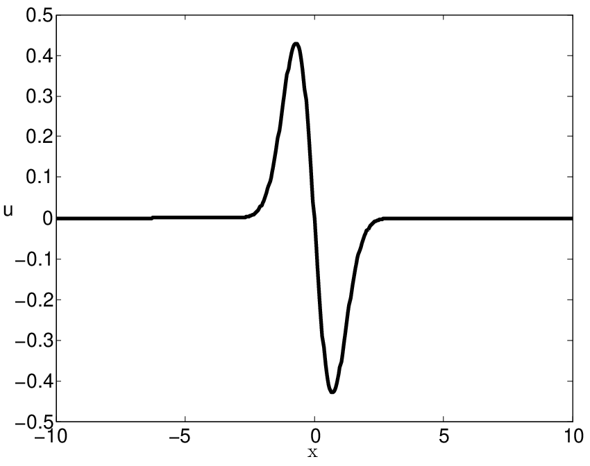
Refer to caption
Refer to caption
Figure 8. Collision of smooth traveling waves: Initial data (left) and exact solution at time T=11T=11.

In order to get a better understanding of this problem, we look at the evolution of the waves with time. Figure 9 shows this evolution together with a zoom close to the collision time.

Refer to caption
Refer to caption
Figure 9. Collision of smooth traveling waves: Evolution in time (left) and zoom of the evolution close to the collision.

We now present the results given by the numerical schemes with grid parameters Δ​ξ=0.25\Delta\xi=0.25 and Δ​t=0.1\Delta t=0.1 in Figure 10.

Refer to caption
Figure 10. Collision of smooth traveling waves: numerical solutions at time T=11T=11. Dashdotted line=ODE45, Stars=Explicit Euler, Diamond=Strang.

We have also checked that only the splitting schemes preserve the positivity of the particle density and conserve the invariants of our problem. Finally, in Figure 11 we display, with the same parameter values as above, the evolution in time of the energy density along the numerical solution given by the Strang splitting scheme. We can observe the concentration of the energy and then its separation in two parts, following the waves.

Refer to caption
Refer to caption
Figure 11. Evolution of the energy density (left picture) along the numerical solution given by the Strang splitting and close up look at the blow up time (right).

With all these numerical observations, we can conclude that the proposed spatial discretisation is robust and qualitatively correct. The time integrators are relatively comparable but only the splitting schemes have the additional properties of maintaining the positivity of the energy density and conserve exactly the invariants of our partial differential equation.

References

  • [1] T. B. Benjamin, J. L. Bona, and J. J. Mahony. Model equations for long waves in nonlinear dispersive systems. Philos. Trans. Roy. Soc. London Ser. A, 272(1220):47–78, 1972.
  • [2] R. Camassa and D. D. Holm. An integrable shallow water equation with peaked solitons. Phys. Rev. Lett., 71(11):1661–1664, 1993.
  • [3] G. M. Coclite, H. Holden, and K. H. Karlsen. Global weak solutions to a generalized hyperelastic-rod wave equation. SIAM J. Math. Anal., 37(4):1044–1069 (electronic), 2005.
  • [4] D. Cohen and X. Raynaud. Geometric finite difference schemes for the generalized hyperelastic-rod wave equation. J Comput Appl Math, 235(8):1925–1940, 2011.
  • [5] A. Constantin and W. A. Strauss. Stability of a class of solitary waves in compressible elastic rods. Phys. Lett. A, 270(3-4):140–148, 2000.
  • [6] H.-H. Dai. Exact travelling-wave solutions of an integrable equation arising in hyperelastic rods. Wave Motion, 28(4):367–381, 1998.
  • [7] H.-H. Dai. Exact travelling-wave solutions of an integrable equation arising in hyperelastic rods. Wave Motion, 28(4):367–381, 1998.
  • [8] H.-H. Dai and Y. Huo. Solitary shock waves and other travelling waves in a general compressible hyperelastic rod. R. Soc. Lond. Proc. Ser. A Math. Phys. Eng. Sci., 456(1994):331–363, 2000.
  • [9] E. Hairer, C. Lubich, and G. Wanner. Geometric Numerical Integration. Structure-Preserving Algorithms for Ordinary Differential Equations. Springer Series in Computational Mathematics 31. Springer, Berlin, 2002.
  • [10] David Henry. Compactly supported solutions of the Camassa–Holm equation. J. Nonlinear Math. Phys., 12(3):342–347, 2005.
  • [11] H. Holden and X. Raynaud. Global conservative solutions of the generalized hyperelastic-rod wave equation. J. Differential Equations, 233(2):448–484, 2007.
  • [12] J. Lenells. Traveling waves in compressible elastic rods. Discrete Contin. Dyn. Syst. Ser. B, 6(1):151–167 (electronic), 2006.
  • [13] T. Matsuo and H. Yamaguchi. An energy-conserving galerkin scheme for a class of nonlinear dispersive equations. J. Comput. Phys., 228(12):4346–4358, 2009.
  • [14] X. Raynaud. On a shallow water wave equation. Ph.D Thesis, 2006.
  • [15] Z. Yin. On the Cauchy problem for a nonlinearly dispersive wave equation. J. Nonlinear Math. Phys., 10(1):10–15, 2003.