∎
The Infrared Behaviour of the Pure Yang-Mills Green Functions
Abstract
We review the infrared properties of the pure Yang-Mills correlators and discuss recent results concerning the two classes of low-momentum solutions for them reported in literature, i.e. decoupling and scaling solutions. We will mainly focus on the Landau gauge and pay special attention to the results inferred from the analysis of the Dyson-Schwinger equations of the theory and from “quenched” lattice QCD. The results obtained from properly interplaying both approaches are strongly emphasized.
Keywords:
Yang-Mills QCD infrared Green functions DSEs Lattice QCD Slavnov-Taylor Ids.1 Introduction
The whole set of correlation functions fully describes a Quantum Field Theory, as it is related to the S-matrix elements. In QCD or pure Yang-Mills theories Green functions are most often gauge dependent quantities which have no direct relationship with physical observables, the latter being necessarily gauge invariant. However, their indirect physical relevance is well known. In particular, long distance (or small momentum) Green functions will hopefully shed some light on the deepest mysteries of QCD such as confinement, spontaneous chiral symmetry breaking, etc.
Indeed, more than thirty five years after the discovery of QCD and notwithstanding its numerous successes, notwithstanding either the fact that everybody is convinced that QCD implies confinement, a real proof of it from first principles has not yet been achieved. This is doubtless one of the major scientific challenges of this century. In fact, in the case of QCD, one is not even provided with a precise mathematical formulation of confinement. In the case of the pure Yang-Mills theory, such a mathematical formulation at least exists: it is the area-law for Wilson loops which unluckily does not hold for QCD due to the string breaking by the sea quarks. Furthermore, the Polyakov loop (the product of link variables along a curve in time direction closed by periodic boundary conditions), probing the screening properties of a static colour triplet test charge, appears to be the order parameter for the deconfinement phase transition. Here we will restrict ourselves to the pure Yang-Mills theory. We will not enumerate all the tracks which have been followed to understand confinement by means of the peculiarities of QCD in the infrared domain, there are many of them (see, for instance, the classical Wilson’s [1] or Cornwall’s [2] works, or the very recent introduction to the confinement problem in ref. [3] and references therein). In this review we will only mention the Kugo-Ojima and the Gribov-Zwanziger approaches. The latter aimed in principle to deal with the problem of Gribov copies, but it is also thought to be connected with confinement scenarios. Both approaches are related to the behaviour of the Green functions of the gluons and ghosts in the deep infrared.
It is now well established that the vacuum of a quantum field theory is never trivial, and especially not in the case of a non-Abelian gauge theory. It is believed that the low modes of the vacuum, the condensates, are the keys to understand its non-perturbative properties. The vacuum is a gauge invariant state. But the configurations of the fields in the vacuum have different features in different gauges. This allows for different, complementary and rewarding views into its properties. We will address this issue (sec. 3.8).
We will concentrate our efforts on a review of the gluon and ghost Green functions properties at small momentum in a pure Yang-Mills theory. We will invoke results from the analysis of Dyson-Schwinger equations (DSE), Slavnov-Taylor identities (ST) and from lattice QCD, paying special attention to the interplay of all these techniques and particularly to the study of Yang-Mills solutions when lattice results happen to be applied as DSE inputs.
We work hereafter mainly in the Landau gauge, but some of the results we will present are actually valid in any covariant gauge. We will also discuss some results in Coulomb gauge and focus especially on the similarities of the general properties of the solutions in both Landau and Coulomb gauges.
Our notations will be the following :
| (1) | |||||
| (2) | |||||
| (3) | |||||
| (4) | |||||
respectively for the ghost propagator, the gluon propagator, the three-gluons vertex and the ghost-gluon vertex11 1 We stick to the decomposition given in ref. [4] except for the arguments of the scalar functions, for which we keep the same order as in itself . All momenta are taken as entering. In eq. (4) is the momentum of the outgoing ghost, the momentum of the incoming one and the momentum of the gluon. corresponds to the gluon-transverse (longitudinal) form factor that will be extensively invoked in the following. is the bare coupling that should be properly renormalized 22 2 By , where () is the gluon (ghost) propagator renormalization constant and is the proper ghost-gluon vertex renormalization constant. and, in the limit of vanishing incoming ghost momentum (), one has
| (5) |
which gives the running coupling in the Taylor renormalization scheme, where and , defined by Eqs.(1,2), are the dressing functions of the ghost and gluon propagators respectively. Up to logarithms, we parametrise the propagators in the infrared by setting at leading order
| (6) |
where are some dimensional parameters. Finally we shall set
As we mentioned, our goal will be to describe the current state-of-the-art concerning the low-momentum properties of the Green functions in gluo-dynamics, mainly by focussing on the results obtained with two main approaches: DSEs and Lattice QCD. The paper is organized as follows: a first section (sec. 2) will be devoted to provide the reader with a first insight on the problem of the Yang-Mills Green functions low-momentum behaviour through reviewing the main analytical properties recently derived in the literature for the solutions; we will review then, as exhaustively as possible, the numerical lattice QCD results on the subject in sec. 3; the results obtained from the numerical resolution of DSEs, with different truncation approaches, will be discussed and put in connection with lattice results in sec. 4; and we finally conclude in sec. 5. However, we will start now by “saying” a few words to introduce those two main approaches and their results, but also about other approaches as the ones based on redefining the QCD lagrangian to properly correct the Gribov ambiguity.
1.1 Lattice results
The lattice technique in gauge field theories was initiated by Wilson in 1974. It has now been used for the field of Yang Mills Green’s functions for nearly 25 years. Let us begin by recalling what it consists in. The general idea is to rewrite the lagrangian on a discretised space-time (the lattice) instead of the ordinary continuous one. Accordingly all derivatives (including the covariant derivatives) are replaced by finite differences. If in addition one limits oneself to a finite volume, the path integral is now over a finite (but huge) number of field variables and can be estimated as a sum over a stochastically determined set of configurations. The advantages are well known :
-
The only ingredient is the original lagrangian, excluding any additional hypothesis. So, in some sense, the results obtained in this way can be considered as exact from the theoretical point of view.
-
The technique is essentially non-perturbative.
-
The lattice spacing acts as an ultraviolet cutoff : no divergence occurs. The continuum limit can be recovered by letting go to zero, at the price of an appropriate renormalisation.
There are some drawbacks to the method, however.
-
It is very demanding in computing power.
-
The results are given in numerical form and, as such, they suffer from uncertainties. The first one is of statistical nature and stems from the finite number of configurations which are used in the evaluation ; it can in principle be reduced at will by increasing this number. The other sources are more intrisically related to the technique, they give rise to systematic errors. We mention them briefly below although they will be discussed in greater detail in dedicated sections in the following (see section 3.5).
First of all the actual calculations are necessarily performed at finite values of the lattice spacing. Naïvely, at tree level, the discretisation procedure generates effects of order in the fermionic lagrangian and of order in the Yang-Mills one. The gap between those conditions and the continuum limit can be partly reduced by using an improved lagrangian (see for instance refs. [5] for the fermionic case and [6; 7; 8] in the pure gauge one). The remaining part has to be treated numerically.
Second, going to the lattice implies, as we have already said, that one works in a finite volume. This induces, in turn, a spacing in -space. Since we are interested in the infrared limit of the Green’s functions we shall have to take special care of potential discontinuities in the neighbourhood of .
Third, the space on which we are working is actually a torus since the field configurations are usually chosen to be periodic. One can therefore wonder what kind of relationship the functions obtained in this way entertain with the “real world” ones.
As a final remark, we note that the Gribov copies problem, which is absolutely general, can be specifically dealt with on the lattice. The gauge fixing procedure consists in gauge-transforming the field configuration into one of its gauge equivalents which satisfy the given gauge condition. Generally the different possible choices do not contribute equally to the path integral. It is therefore an important issue to know how large this effect is and how one can minimize it. Within the numerical precision, this can be explicitely done on the lattice, as will be discussed in section 3.6.
The number of papers dealing with lattice simulations for Green functions in the IR is rather large, and their results are given according to quite a variety of presentations, which makes the task of comparing them not so easy. We shall try to give an account of those works in sec. 3. Note that the most recent studies have been performed in the unquenched theory ([9; 10; 11; 12]), so that they fall out of the scope of this review and will not be discussed.
1.2 The DSE picture
In principle, the field equations for the Green functions of a quantum field theory can be derived from the integral representation of the theory; these are the Dyson-Schwinger equations (DSEs) of this theory which are considered to describe its non-perturbative dynamics [13; 14]. Under the only assumption of the existence of a well-defined measure in a functional integral representation of the generating functional for the Green functions of a theory, QCD for instance, the corresponding DSEs can be derived (see for instance [15]) as an infinite tower of coupled integral equations. Of course, in practice, these equations need to be truncated to be studied. Typically, one can make appeal to additional sources of information, for instance Slavnov-Taylor identities, to express higher -point functions in terms of elementary two-point ones or to generate some general ansätze for vertices. Thus, a closed coupled system of DSEs is to be obtained and can be numerically solved, subject to the validity of the truncation rules which are applied. This DSE approach has been extensively applied to investigate the low-momentum behaviour of the QCD Green functions; in particular, for the Yang-Mills gluon and ghost propagators. We will dedicate secs. 2 and 4 to describe some of the main results contributing to the current DSE picture for this low-momentum behaviour of Yang-Mills Green functions. Let us however briefly introduce those results and how they emerged in the last few years.
After the first pioneering works of Mandelstam [16; 17] and the further ones of Brown and Pennington [18], only a few years ago, a new paradigm emerged when it was widely accepted (see for instance [15]) that a vanishing gluon propagator and a diverging ghost dressing function at zero-momentum in Landau gauge made up the unique solution of the truncated tower of DSEs. In contrast, alternative DSE solutions were also predicted to give a massive gluon propagator [19; 20]. Lattice QCD (LQCD) estimates for those propagators appeared to be also in contradiction with a gluon propagator that vanishes at zero-momentum or with a ghost dressing function that diverges [21; 22; 23; 24; 25]. We addressed this issue in two recent papers [26; 27] and tried to clarify the contradiction. After assuming in the vanishing momentum limit a ghost dressing function behaving as and a gluon propagator as (or, by following a notation commonly used, a gluon dressing function as ), we proved that the ghost propagator DSE (GPDSE) admits two types of solutions:
-
If , the low-momentum behaviour of both gluon and ghost propagators are related by the condition implying that goes to a non-vanishing constant when . This solution is now called “scaling”.
-
If , the low-momentum leading term of the gluon propagator is not constrained any longer by the leading but instead by the next-to-leading one of the ghost propagator, and LQCD solutions indicating that when [23; 24] can be pretty well accommodated within this case. This solutions is named as “decoupling”.
In particular, the numerical study in ref. [26] of the GPDSE using a LQCD gluon input finds that two classes of solutions emerge, depending on the value of the strong coupling constant at the renormalization point, which is a free parameter in this exercise. Indeed, it seems to be by now well established that the two classes of solutions, decoupling and scaling may emerge from the tower of DSE [19; 20; 28]. Such a nomenclature, despite being widely accepted, can be misleading. The perturbative running for the coupling constant renormalized in Taylor-scheme is given by Eq. (5) and one can thus extend this definition, although not univocally, to the IR domain. However, a scale invariance ( a decoupling) of the IR dynamics for the theory cannot be inferred from the low-momentum behaviour of such a coupling in the scaling (decoupling) solution. In particular, as will be seen in next Eq. (70) of subsection 2.2 (see also Eqs. (2.30-2.32) in ref. [29]), an effective charge can be properly defined for phenomenological purposes such that it reaches a constant at zero-momentum in the “decoupling” case, which means the absence of decoupling. Leaving aside nomenclature, the two classes of solutions are definitely different and the Taylor-scheme coupling, although maybe not appropriate for phenomenological purposes in the IR domain, is a well defined and very convenient quantity to discriminate them.
How both types of IR solutions for Landau gauge DSE emerge and how the transition between them occurs, in relation with the size of the coupling (taken as an integration boundary condition at the renormalization momentum), was initially discussed in ref. [26] through the analysis of a ghost propagator DSE combined with a gluon propagator taken from lattice computations. It should be remembered that one needs to know the QCD mass scale to predict the QCD coupling at any momentum. This mass scale should be of course supplied to get a particular solution from DSE and can be univocally related to the boundary condition needed, after applying a truncation scheme, to solve the equation. The existence of a critical value for the coupling at any renormalization momentum was suggested by that partial analysis. No solution was proven to exist for any coupling bigger than the critical one and the unique scaling solution33 3 The authors of [30] proved there, once the scaling behaviour is assumed, the uniqueness for Yang-Mills infrared solutions seemed to emerge when the coupling took this critical value. Later, the authors of ref. [28] confirmed, by the analysis of the tower of DSE truncated within two different schemes and also in the framework of the functional renormalization group, that the boundary condition for the DSE integration determined whether a decoupling or the scaling solution occurs. A similar analysis has been recently done in the Coulomb gauge [31] leading to the same pattern as in ref. [26], although the authors interpret the boundary condition in terms of the gauge-fixing ambiguity (see also [32; 33]). Furthermore, an analytic study based on the pinch technique (PT) in ref. [34] shows that, within some approximations, there is a lower limit for the gluon mass, below which the PT coupling is singular in the IR, that can be also interpreted as an upper limit to the coupling at some renormalization point. Very recently also, a next-to-leading low-momentum asymptotic formula for the decoupling ghost dressing function solutions was obtained by studying the ghost propagator DSE under the assumption, for the truncation, of a constant ghost-gluon vertex and of a simple model for a massive gluon propagator [35]. In this asymptotic formula, the ghost-propagator low-momentum behaviour appears to be regulated by the zero-momentum effective charge in Taylor scheme [29] and by the Landau-gauge gluon mass scale.
That DSEs, being an intricated tower of coupled functional differential equations, admit multiple solutions belonging to different types is not very surprising. The curent lattice results appear to be clearly compatible with only one type of solutions and, after the appropriate physical calibration of the simulations has been performed (and all the lattice artefact have been put properly under control), must help to select the “physical” solutions for the QCD Green functions among the multiple DSE ones. Furthermore, as will be discussed in the next subsection, an effective action incorporating the so-called Gribov horizon can be properly built to deal with the Gribov problem, and the lattice-like solutions can also appear as those minimizing this effective action (the emergence of non-vanishing dimension-two condensates, that we will also discuss in section 3.8, plays a crucial role in obtaining the lattice-like solutions).
1.3 The Gribov and the Gribov-Zwanziger approaches
The computation of gauge dependent quantities like the correlation functions we are interested in suffers from the Gribov ambiguity: imposing a constraint like the Landau gauge condition is not enough to pick unambiguously a unique representative from each gauge orbit [36]. Gribov then proposed to reinforce the gauge condition by restricting the space of gauge fields to representatives minimizing the functional
| (7) |
where is the gauge transformed field. This is appealing from two points of view : first the Gribov problem is reduced as gauge copies which are maxima or saddle points of are pushed out of the game and second this restricted space, named the Gribov region, is rather easy to characterize mathematically. Actually the second derivatives of the functional defines an operator, the so-called Fadeev-Popov operator, which has to be positive in the Gribov region. For the Landau gauge this operator reads :
| (8) |
where is the covariant derivative. But in general along a gauge orbit the minimum for the functional is not unique. The ambiguity in the gauge fixing is not fully eliminated this way. It is then natural to try to restrict further the space of gauge fields to configurations which are not only a minimum but an absolute minimum of . This region, named the fundamental modular region, in which on each gauge orbit F possesses a unique absolute minimum (cf reference [37]), would be theoretically convenient to eliminate the Gribov problem but unfortunately no practical explicit characterization has been found so far.
Gribov proposed a heuristic method to perform the restriction to the Gribov region. He computed the inverse of the Faddeev-Popov operator in perturbation theory at one loop and found an expression with a structure like :
| (9) |
The explicit form for can be found in the original paper by Gribov but is not necessary for the general discussion here. The Gribov region is a space where the eigenvalues of the Fadeev-Popov operator are positive. Forbidding the crossing of the boundary of this region is equivalent to forbid the appearance of a zero eigenvalue. This is the origin of a condition proposed by Gribov to restrict the space of gauge fields to the Gribov region :
| (10) |
With this restriction as a constraint, Gribov computed the ghost and the gluon propagators (at one loop) and found :
| (11) | |||||
| (12) |
Namely, when goes to 0, a vanishing gluon propagator and an enhanced ghost propagator are exhibited. is called the Gribov mass.
One step further has been accomplished by Zwanziger [38] to relax the approximation used in the determination of the constraint and to extend it to all orders. He found a condition to restrict the space of gauge fields [38]
| (13) |
where , the horizon function , is a non local functional of the gauge fields. This approach has been subsequently refined and developed by Zwanziger himself ([39]) and other authors ([40; 41; 42; 43]). Zwanziger showed that this condition can be exponentiated to be transformed into a contribution to the action :
| (14) |
to be added to the usual contributions coming from the gauge action and the gauge fixing terms. is defined by a relation, the horizon condition, required to implement the exponentiation :
| (15) |
This action has many interesting properties : auxiliary fields can be introduced to transform in a local form [44] ; the theory has been proven to be renormalizable [44] ; the gluon and ghost propagators have been computed and results similar to the Gribov ones are found: a vanishing gluon propagator and an enhanced ghost propagator. These results were in accordance with the common prejudice inferred at that time from the Dyson-Schwinger equations.
As it became clearer and clearer that the lattice results for the propagators were not in accordance with these predicted behaviors, a refined version of the GZ approach was necessary to have an answer for this discrepancy. The key point is the explicit introduction of the dimension two condensates [41; 43]. This has the very nice feature that the renormalizability is not spoiled. With this refinement the gluon and ghost propagators are in qualitative agreement with the lattice results and the prediction from the “decoupling” solution of the Dyson-Schwinger equations. In particular, the gluon propagator in the so-called “refined” Gribov-Zwanziger (RGZ) formalism is shown to behave as
| (16) |
where is the Gribov-Zwanziger parameter determined by the horizon condition, Eq. (15), while and are two mass parameters related to the two above mentioned condensates . In particular, is related to the dimension-two gluon condensate, , that will be discussed in detail below (cf. section 3.8) and plays a crucial role for the RGZ gluon propagator to account for lattice results [45]. Furthermore, the authors of ref. [46] studied the effective action in RGZ and provided firm evidences that the dimension-two condensates should be non-vanishing (and hence the mass parameters and ) and a strong indication that, in addition to the non-zero gluon propagator at vanishing momentum, the ghost propagator is not enhanced, in consistence with lattice data and with the previously discussed DSE picture for decoupling solutions.
1.4 Other approaches
Many other approaches have been applied to investigate the low-momentum properties of the Yang-Mills Green functions. We will end this introduction by indicating some of them and addressing the interested reader to some original works. Apart from DSEs or Lattice QCD, one of the most followed approaches is that of functional renormalization group equations (FRGs) [47; 48; 49; 50; 51]. Indeed, FRGs and DSEs appear to be rather interconnected and, for instance, it has been shown that the integrated flow equations define a set of DSEs within a particular renormalization scheme [51]. First, it was reported that FRGs analysis of the Landau-gauge low-momentum behaviour for the Yang-Mills Green functions leads to the uniqueness of a scaling-type solution [50; 30], but it has been recently proven, also within FRGs, that both scaling and decoupling solutions exist [52]. On the other hand, other approaches like the infrared mapping of and Yang-Mills theories in ref. [53; 54; 55] or the massive extension of the Fadeev-Popov action in ref. [56; 57] appear to support a massive gluon propagator and a free ghost, i.e. a decoupling-type solution. In particular, a very accurate description of lattice data for Yang-Mills gluon and ghost correlators in Landau gauge is obtained by means of a one-loop computation with this last massive extension of the Fadeev-Popov action in four dimensions, while the main features for lattice results in d=2,3 can be also accounted for. Furthermore, the low-momentum behaviour for the one-loop results with this massive action matched pretty well with the one expected for a decoupling solution within DSEs approach. One can find in the literature still other methods, such as the application of stochastic quantization [58; 59], that have been applied to the subject.
1.5 The low-momentum correlators and the confinement problem
Let us end this introduction with one comment about the Kugo-Ojima [60] confinement criterion which might be in order here. In the Kugo-Ojima colour confinement picture, the physical spectrum of the theory is free of coloured asymptotic states as a consequence of the so-called “quartet mechanism”. A sufficient condition for it to take place is that a certain correlation function, usually denoted by and called “Kugo function”, should satisfy . Furthermore, in Landau gauge, the Kugo function is linked to the ghost dressing function such that (This relation was first noted by T. Kugo [61] and very recentely, K-I. Kondo triggered an interesting discussion about this relation, in connection with the Gribov horizon condition and its implications on the Landau-gauge Yang-Mills infrared solutions [40; 62]). Therefore, the sufficient condition for the realization of Kugo-Ojima confinement scenario requires a divergent ghost dressing function. Then, for the two classes of solutions above discussed, only the scaling may satisfy this sufficient condition. A different mechanism should thus explain the confinement for decoupling solutions, as for instance the one provided by the center vortices scenario [2; 63; 64].
However, as stated in the brief review about “Strong Coupling Continuum QCD” recentely appeared in the proceedings of the 9th conference on “Quark Confinement and the Hadron Spectrum” [65], the physics of hadrons and the confinement do not depend very much on how gluon and ghost propagates over distances of atomic scales but mainly on those of the size of a nucleus, where the difference between scaling and decoupling solutions is not important. Thus, it is very reasonable to think that the real QCD confinement mechanism might not be of a great help to discriminate among the two types of low-momentum solutions.
2 A first insight with analytical tools
2.1 The low momentum solutions from the ghost propagator DSE
2.1.1 The ghost propagator DSE
We will examine the Dyson-Schwinger equation for the ghost propagator (GPDSE) which can be written diagrammatically as
i.e., denoting by (resp. ) the full ghost (resp. gluon) propagator,
| (17) | |||||
where stands for the bare ghost-gluon vertex (above defined in Eq. (4)),
| (18) | |||||
while and are respectively the outgoing and incoming ghost momenta and is the bare coupling constant. Let us now consider eq. (17) at small momenta . After applying the decomposition for the ghost-gluon vertex in eq. (18), omitting colour indices and dividing both sides by , it reads
| (19) |
It should be noticed that, because of the transversality condition, defined in eq. (18) does not contribute for the GPDSE in the Landau gauge.
2.1.2 Renormalization of the Dyson-Schwinger equation
The integral equation eq. (19) is written in terms of bare Green functions. It is actually meaningless unless one specifies some appropriate UV-cutoff,44 4 We have written for simplicity the UV cutoff as a hard cut-off. It is preferable to use a gauge invariant regularization procedure in view of the advantage of exploiting Ward-Slavnov-Taylor identities (see sec. 2.3). In practice we will derive our results from the subtracted GPDSE which incorporates gauge invariant UV regularisation. , and performs the replacements … . It can be cast into a renormalized form by dealing properly with UV divergences, i.e.
| (20) |
where is the renormalization momentum and and the renormalization constants for the coupling constant, the gluon and the ghost respectively. is related to the ghost-gluon vertex renormalization constant (defined by ) through . Then Taylor’s non-renormalization theorem, which states that in Landau gauge (see app. A) and to any perturbative order, can be invoked to conclude that is finite. We recall that the renormalization point is arbitrary, except for the special value which cannot be chosen without a loss of generality (see, in this respect, the discussion in ref. [66]). Thus,
| (21) |
where
One should notice that the UV cut-off, , is still required as an upper integration bound in eq. () since the integral is UV-divergent, behaving as . In fact, the cut-off dependence this induces in cancels 55 5 One can easily check that approaches some finite limit as since the ghost and gluon propagator anomalous dimensions and the beta function verify the relation [67]. against the one of in the r.h.s. of eq. (21), in accordance with the fact that the l.h.s. does not depend on .
Now, we will apply a MOM renormalization prescription. This means that all the Green functions take their tree-level value at the renormalization point and thus:
| (23) |
In the following, will be approximated by a constant66 6 This approximation is very usually used to solve GPDSE. Some lattice data are available for the ghost-gluon vertex, although they are by far less numerous than the ones regarding the propagators (see section 3.2).The present data do indicate that the zero gluon momentum is approximatively constant with respect to [23]. Of course, more data for different kinematical configurations should be welcome to check that approximation. with respect to both momenta and, provided that at tree-level, our MOM prescription implies that and is a constant in terms of .
2.1.3 A subtracted Dyson-Schwinger equation
The renormalized GPDSE, eq. (21), should be carefully analysed. We aim to study the infrared behaviour of its solutions and therefore focus our analysis on the momentum region, , where the IR behaviour of the dressing functions (presumably in powers of the momentum) is supposed to hold. One cannot forget, though, that the UV cut-off dependences in both sides of eq. (21) match only in virtue of the previously mentioned relation between the ghost and gluon propagator anomalous dimension and the beta function.
However, in order not to have to deal with the UV cut-off, we prefer to approach the study of the GPDSE in the following manner: we consider eq. (21) for two different scales, and (with some fixed number and an extra parameter that we shall ultimately let go to 0) and subtract them
| (24) |
Then the integral in the r.h.s. is UV-safe, thanks to the subtraction, and the limit can be explicitely taken,
| (25) | |||||
This equation is evidently a necessary consequence of the original one (21). That, conversely, it is actually sufficient was shown in [26]. For an accurate analysis of eq. (24) it is convenient, in addition, to split the integration domain of eq. (25) into two pieces by introducing some new scale (, typically of the order of , is a momentum scale below which the deep IR power behaviour is a good approximation),
| (26) |
where represents the integral in eq. (25) over and over . Only the dependence on is written explicitly because we shall let it go to zero with , and kept fixed. The relevance of the scale stems from the drastic difference between the IR and UV behaviours of the integrand. In particular, for , the following infrared power laws,
| (27) |
will be applied for both dressing functions in .
Now, a straightforward power-counting argument shows that is infrared convergent if :
| (28) |
We shall suppose in the following that these conditions are verified. Let us first consider . Its dependence on , which is explicit in the factor inside the square bracket of eq. (25), should clearly be even in : any odd power of would imply an odd power of whose angular integral is zero. Since the integrand is identically zero at and the integral is ultraviolet convergent, it is proportional to (unless some accidental cancellation forces it to behave as an even higher power of ). On the other hand, after performing the change of variable , the IR contribution of the integral in eq. (25)’s r.h.s can be rewritten as:
| (29) | |||||
that, as it shall be seen in the next subsection, asymptotically behaves as
Thus, in all the cases, the leading behaviour of , as vanishes, is given by in eq. (2.1.3). The subtracted renormalised GPDSE reads for as:
| (34) |
for small . We have assumed that is constant when varying all the momenta but (2.1.3,34) remain true if one only assumes that behaves “regularly” for (i.e. is free of singularities or, at least, of any singularity worse than logarithmic).
2.1.4 The integral for the ghost self-energy
The present section is devoted to the quantitative analysis of the integral , defined in Eq. (29), which gives the contribution of the ghost loop to the renormalised GPDSE Eq. (34). If it is possible to perform analytically the integral and to find a compact expression for it. In this case, one can write
| (35) |
where and were defined in Eq. (27) and
| (36) |
provided that is not singular, so that the subtraction inside the bracket and the integral operator in Eq. (35) commute with each other. Then, following [68], we define
| (37) | |||||
and obtain
| (38) |
where
| (39) | |||||
Thus, if ,
| (40) |
We will now compute the leading asymptotic behavior of as when . In that case, after performing in Eq. (29) the following expansion,
| (41) | |||||
and neglecting the term odd in one finds for the leading contribution
| (42) | |||||
We do not specify the lower bound of the integral over in Eq. (42) because it necessarily contributes as a subleading term, once the ghost-loop integral is required to be IR safe. Then, as was indicated in anticipation in Eq. (2.1.3), diverges logarithmically as goes to zero if . In fact, since Eq. (40) is a reliable result for any however close it may be to 1, such a divergence appears as a pole of a function of in Eq. (38).
Finally, if , the leading contribution for as vanishes can be computed after performing back the change of integration variable, , in Eq. (29). The first even term in Eq. (41) dominates again the expansion after integration, but now it does not diverge. Then, if we procceed as we did in Eq. (42), we obtain
| (43) |
for small and . It should be noticed that in Eq. (43) depends on the additional scale introduced in Eq. (26) to separate IR and UV integration domains. In fact, if one takes , diverges. This means that, when , the behaviour of the IR power laws hampers their use for all momenta in the integral. The finiteness of the ghost-loop integral of the subtracted GPDSE can only be recovered after taking into account the UV logarithmic behaviour for large-momenta dressing functions 77 7 The multiplicatively renormalisable (MR) truncation scheme corresponds to letting . Therefore, the scale being of the order of , power laws with cannot be accepted as solutions of the GPDSE (see, for instance, [68]). The same argument holds also for , because the ghost-loop integral in Eq. (42) diverges as for any fixed as well as for for any fixed . . Furthermore, , behaving too as , should also be added in the r.h.s. of Eq. (34) in order to write the renormalised GPDSE. Thus, the dependence on but not the factor in front of it can be inferred from the GPDSE with only the information of the asymptotics for small-momentum dressing functions.
2.1.5 The two classes of solutions
The starting point for the following infrared analysis will be the Eq. (34) for small , where we will try to make the dependences on and of the two sides match each other.
The case (scaling solution):
We will first study the case . Then, the l.h.s. of Eq. (34) can be expanded for small as
| (44) |
and one obtains from Eq. (34):
| (45) |
where the dependences on and of the numerator and the denominator should cancel against each other. Using for the form given after Eq. (2.1.3), we find three possible situations:
An immediate consequence of this last condition is the freezing of the running coupling constant at small momentum. If the renormalization point, , is arbitrarily chosen to be very small in order that the dressing functions observe the power laws at , one obtains and . Eq. (46) then reads
| (47) |
and should be satisfied for any small value of . Consequently, it should remain exact as and provides the small-momentum limit of the running coupling (which is independent of the infrared constants for ghost and gluon dressing functions).
In particular, if , one has and thus
| (48) |
The case (decoupling solution):
The case is particular in that the leading contributions to the two occurrences of in the l.h.s of eq. (34) cancel against each other. We have then to go one step further, taking into account the subleading terms. Defining by means of we rewrite the l.h.s of eq. (24) as and use the known IR behaviour of from eq.2.1.3)) in the r.h.s. of eq. (34) to get
Furthermore, not only the subleading functional behaviour of the dressing function can be constrained but also the coefficient in Eq. (2.1.5). In fact, if we plug this equation into the l.h.s. of eq. (34) and expand we obtain :
Let us consider now in more detail the three possible cases.
-
At last, if , eqs. (43) and (2.1.5) imply: . i.e., a ghost dressing function which behaves quadratically for small momenta, In this case, however, as already said the ghost loop cannot be evaluated using the IR power laws over the whole integration range and it is therefore not possible to solve the GPDSE consistently, nor even to determine the small-momentum behaviour of the dressing functions, without matching appropriately those power laws to the UV perturbative formulas. Thus, we are not able to derive a constraint for the next-to-leading coefficient, .
In summary, the GPDSE admits IR solutions with and any , provided that
where and is given in Eq. (56). The gluon dressing function is supposed to behave as indicated in Eq. (27). In particular for , the gluon propagator takes a finite (and non-zero) value at zero momentum, , after applying MOM renormalisation prescription at .
2.2 The low-momentum solutions and the gluon mass
As will be seen in the next section, the current lattice data strongly supports a decoupling solution which does not obey and in which . Furthermore, lattice data can also be very well accommodated within DS coupled equations in the PT-BFM scheme [19; 20] and within the so-called refined Gribov-Zwanziger approach [42], leading in both cases to decoupling solutions for gluon and ghost propagators. Then, as Eq. (2.1.5) reads for, this implies a ghost dressing function proportional to while the gluon propagator takes a constant at vanishing momentum () or, in other words, is “massive”.
Indeed, it is well known that the Schwinger mechanism of mass generation [69] can be incorporated ino the gluon propagator DSE through the fully-dressed non-perturbative three-gluon vertex and gives rise to the generation of a dynamical gluon mass such that [19; 70],
| (62) |
In particular, it has been shown that a power-law running mass,
| (63) |
appears as a solution for the coupled ghost and gluon propagator DSE in the PT-BFM truncation scheme [71] and, also, as a consequence of the dimension-4 gluon condensate in the OPE expansion of the gluon self-energy in the Pinching Technique framework [72].
Having this in mind, the authors of ref. [35] applied the following simple model 88 8 This is a renormalized massive gluon propagator, as given by Eq. (62), where the gluon running mass appears to be approximated by . This is, for instance, a very good low-momentum approximation for the running mass given by Eq. (63) with GeV and GeV (see fig. 11 of ref. [29]).:
| (64) |
for a massive gluon propagator, in order to compute the -correction for the low-momentum ghost dressing function and then prove that this low-momentum behaviour is controlled by that gluon mass and by the zero-momentum value of the effective charge defined from the Taylor-scheme ghost-gluon vertex in ref. [29].
The work of ref. [35] can be easily overviewed if we re-write Eq. (24) as follows
| (65) | |||||
for the two momenta and , which will be taken to be small (as compared with and , the cut-off separating IR and UV modes in the ghost-self-energy integral), and where the ghost-gluon transverse form factor, , has been explicitly replaced by 1 and the dependence on the renormalization momentum, , omitted by simplicity. Then, if one inserts the form Eq. (64) of the gluon propagator into the integrand and focuses on the low-momentum behaviour of the ghost dressing function for the decoupling case (, the ghost dressing function will be replaced by the constant leading term, from Eq. (27), and one will obtain:
| (66) | |||||
The integral given by Eq. (66) can be first analytically obtained and then expanded up to the first order in to give:
| (67) | |||||
from where one needs only to keep
| (68) |
because the terms in are neglected, while the constant terms and the ones logarithmically divergent () happen to be cancelled when applying the subtraction for two different momenta in the r.h.s. of Eq. (65).
Thus, if one replaces by the result of Eq. (68) in the r.h.s. of Eq. (65), the subleading term for the ghost dressing function should be:
| (69) |
where:
| (70) | |||||
Here is the perturbative strong coupling defined in the Taylor scheme [73], while is the non-perturbative Taylor effective charge defined as an extension of the Taylor ghost-gluon coupling in ref. [29], similarly to the way the ‘‘pinching technique’’ 99 9 The “pinching technique” [70] implies a resummation of the diagrams for the perturbative gluon propagator expansion leading to a redefinition of the propagator such that it observes a QED-like Ward identity, thus providing us with a way to construct an IR effective charge as happens in QED. (PT) effective charge was from the gluon propagator in ref. [74].
2.3 Some constraints from Slavnov-Taylor identities
In the previous section, we have analysed the infrared behaviour of the GPDSE solutions and found that the ghost dressing function can either diverge at vanishing momentum ( with ) or take a finite value ( with any ). As appendix B shows, the GPDSE themselves can be derived from the general Ward-Slavnov-Taylor equation [75]. The Ward-Slavnov-Taylor identities (WSTI) can be derived formally from the gauge invariance of the path integral, eq. (137) of appendix B, as shown in [76]. This is the case in lattice simulations. If the path integral is limited to a domain of the configuration space such as in the Gribov-Zwanziger approach, used in [42], the STI may not be satisfied. We assume a gauge invariant path integral and will now invoke the WSTI for general covariant gauges relating the 3-gluon, , and ghost-gluon vertices,
| (71) |
to shed some light on that matter [77; 78]. Using for the ghost-gluon vertex the general decomposition1010 10 We work, of course, on the energy-momentum shell, so that the relation holds [79]
| (72) | |||||
and multiplying by both sides of Eq. (71), one obtains:
| (73) |
where
| (74) |
Since the vertex function, , in the l.h.s. of Eq. (73) is antisymmetric under and , one can conclude that[4; 77]:
| (75) |
This last result is a compatibility condition required for the WSTI to be satisfied that does not involve the 3-gluon vertex and implies a strong correlation between the infrared behaviours of the ghost-gluon vertex and the ghost propagator. Now, under the only additional hypothesis that those scalars of the ghost-gluon vertex decomposition in Eq. (72) which contribute to the scalar function defined in Eq. (74) are regular1111 11 Note also that, for our purposes, it will actually be enough to restrict, but not forbid, the possible presence of singularities in the scalar coefficient functions provided that they could be compensated by kinematical zeroes stemming from the tensors. when one of their arguments goes to zero while the others are kept non-vanishing, one can consider the small limit in Eq. (75) and obtain:
| (76) |
This has to be true for any value of , which implies that goes to some finite and non-zero value when goes to zero, since neither nor are presumably zero for all values of . Rephrased in terms of infrared exponents, the latter argument implies that .
To reach the above conclusions we did not appeal to the properties of the 3-gluon vertex, apart from the symmetry under the exchange of gluon legs. If one assumes in addition that the longitudinal part of the 3-gluon vertex also behaves regularly when anyone of its arguments goes to , the others being kept non-vanishing, a divergent gluon propagator at vanishing momentum will be obtained from Eq. (73) [24; 80; 77]:
| (77) | |||||
implying that
| (78) |
Of course, as far as it involves a vertex with longitudinal gluons which have not been very extensively studied, this last conclusion is not as clean as the previous one about the ghost dressing (according to authors of ref. [81] a soft kinematical singularity appears for the landau-gauge 3-gluon vertex, however it does not concern our proof relying on the regularity of the longitudinal-longitudinal-transverse 3-gluon vertex).
In ref. [77], we showed that only a very mild divergence, for example of logarithmic type, could be compatible
(although very unlikely) with current LQCD results for the gluon propagator. The IR analysis of the previous section can be straightforwardly extended to this case by generalizing
| (79) |
the effect of which is to modify Eq. (2.1.5) with
where only the power of the logarithm is then modified.
Sticking now to the case where is zero (for the reasons explained above) and is 1 (as suggested by the lattice results) we are left with
| (84) |
according to whether there are logarithmic corrections to the gluon propagator () or not (). Here, is some scale which is out of the scope of the IR analysis we performed in the previous section and, if , is the gluon propagator at zero momentum.
3 Low-momentum Green functions lattice results
As was recalled in the previous section, the mechanisms usually invoked to explain the confinement imply specific behaviours in the infrared for the Green’s functions of the theory :
-
A sufficient condition for the Kugo-Ojima criterion1212 12 The Kugo-Ojima scheme also implies that there be no massless pole in the transverse gluon propagator (cf [61]), a condition which is weaker than the vanishing advocated in the Gribov-Zwanziger scenario. to be satisfied would be the divergence of the ghost dressing function, as (see ref. [60; 61])
-
The Gribov-Zwanziger scenario implies the vanishing of the gluon propagator. i.e. as (ref [82])
In addition, the dressing functions should obey Dyson-Schwinger equations, from which it was inferred that the ghost and gluon infrared exponents (cf. equation (6) above) should satisfy the relation (referred to in the following as Rel) Accordingly Zwanziger [59] and Lerche and von Smekal [66] predicted a value
Since those results rely on theoretical conjectures and since using the Dyson-Schwinger equations demands an unescapable and not fully controlled truncation of their infinite tower, the technique of lattice simulations has become an alternative and totally independent means to get reliable model-independent information on the Green’s functions. The first attempts to measure propagators took place at the end of the eighties for the gluon [83; 84; 85] and in the second half of the nineties for the ghost [86; 87; 88]. Since then, thanks to the huge increase in the performance level of the computers, it has become possible to reach larger volumes while keeping a small enough lattice spacing. This circumstance is essential to get an ever more detailed insight in the infrared behaviour of the propagators and vertices.
The simulations have been performed using a variety of setups :
-
dimensionality of the space, ranging from 2 to 4. The relation (Rel) is actually the restriction to the case of a more general -dependent one.
-
choice of the gauge action : either standard Wilson or improved versions, quenched or unquenched.
-
lattice geometry (isotropic or not), spacing, lattice size.
We present in this section an overview of the results of these simulations, with emphasis on the case of an gauge group and of the pure Yang-Mills theory (quenched QCD). The case of the gauge group has been considered very thoroughly by Cucchieri and Mendes (see for instance [89] and the references therein). A comparison of the dressing functions for and has been performed in ref. [25] and shows that the dressing functions are remarkably close for both the gluon and the ghost, in accordance with the theoretical expectations.
3.1 Ghost and gluon propagator results in Landau gauge
We summarize in table 1 the results concerning the IR properties of the propagators which have been reported in the literature. They are usually, but not always, given in terms of values of the exponents and . The reader should keep in mind that in many of the latter cases, the authors have attempted to describe both the gluon and the ghost propagator with only one parameter, automatically taking into account the relation (Rel), but simultaneously introducing some kind of bias in the fit, all the more as, as we shall see, this relation is not satisfied by the data. Actually such a one-parameter fit revealed impossible in several cases [90].
| Ref | year | Lat. Size | gluon | ghost | |
| [91; 92] | 2001 | 5.7 | |||
| -id- | -id | 4.38(+) | |||
| -id- | -id | 3.92(+) | finite | ||
| -id- | -id | 3.75(+) | non zero | n.m. | |
| -id- | -id | 3.92(+) | |||
| -id- | -id | 4.1(+) | |||
| -id- | -id | 6.0 | |||
| [93] | 2005 | 5.8 | |||
| -id- | -id | 6.0 | decreases | ||
| -id- | -id | 6.2 | with | ||
| [24; 94] | 2005 | 5.75 | |||
| [95; 96] | 2006 | 6.0 | n.m. | ||
| [97] | 2006 | 5.8 | finite | ||
| -id- | -id | 6.0 | non-zero. | or | |
| -id- | -id | 6.2 | D(0) | log-like | |
| [22] | 2007 | 5.7 | -id- | not power-like | |
| [98] | 2007 | 6.0 | |||
| -id- | -id | -id | not power-like | ||
| -id- | -id | 6.2 | |||
| [99] | 2008 | 6.0 | not | ||
| -id- | -id | -id | conclusive | n.m. | |
| [100; 101] | 2009 | 6.0 | not | n.m. | |
| -id- | -id | 5.7 | conclusive | ||
| [102; 103; 104] | 2009 | 6.0 | |||
| -id- | 2009 | 5.8 | non zero | n.m. | |
| -id | 2009 | 6.0 | D(0) | ||
| [105] | 2009 | 5.7 |
While the first measurements on the lattice resulted in a value of compatible with 2, i.e. with a gluon dressing function behaving as at small ’s [85], the table shows that there is nowadays a general agreement (see also ref. [89]) in favour of a solution incorporating :
- 1.
a gluon dressing function going to 0 like , leading to a propagator remaining finite and non-zero (“massive gluon”)
- 2.
a ghost dressing function going to a non-zero constant, i.e a ghost propagator behaving as (“free ghost”)
Recent numerical data (regarding the quenched case ) on very large lattices are to be found in [105]. They are visualised in figure 1 below, in which the left panel is borrowed from [105]. Similar simulations are now underway for the unquenched cas. The preliminary results appear to be qualitatively compatible with the general picture we have described. We defer the discussion of the different artefacts which can affect the results to a special subsection but, meanwhile we can only make ours the statement of ref. [89] : “ The current paradigm is that of a massive gluon and a free ghost”.
 |
 |
3.1.1 Lattices vs Dyson-Schwinger equations
The fact that the most recent results of lattice simulations, and , were actually compatible with the Dyson-Schwinger equations was first demonstrated in reference [26] by a numerical analysis of the GPDSE where the gluon propagator lattice data were plugged into the kernel and the transverse form factor was supposed to be constant for all momenta. We will come back to this result in sec. 4, where the agreement of lattice data and the numerical DSE results for the decoupling case will be manifest from fig. 7.

Furthermore, as we discussed in the previous section, in the subsection 2.2, the authors of ref. [35] provided us with a low-momentum analytic expression for the ghost dressing function, Eq. (69), derived from the asymptotic analysis of the GPDSE. This result was also succesfully confronted to the lattice data for the ghost propagator dressing, in particular with those obtained from very large lattice 1313 13 These lattice data were also obtained with the SA gauge-fixing algorithm so as to deal as well as possible with the Gribov ambiguity but, for instance in determining the gluon mass by fitting Eq. (69) to the ghost dressing data, some systematic uncertainty should be admitted to come from the gauge-fixing procedure. simulations in ref. [22]; this comparison was performed in [35]. from which we borrow Fig. 2 where the ghost propagator lattice data are shown to behave pretty well as Eq. (69) asks for with a gluon mass, GeV, in the right ballpark (roughly from 400 MeV to 700 MeV) defined by phenomenological tests [106] or direct lattice measurements from the gluon propagator [91; 92; 102; 107].
3.2 The ghost-gluon vertex
Among the numerous possibilities to define the QCD renormalised coupling constant a particularly attractive one, for use in lattice simulations, is based on the ghost-ghost-gluon 3-point function together with a specific -type renormalisation scheme in which the incoming ghost has zero momentum. We have intoduced in eq. (18) the 2 form-factors and of the vertex; in terms of those factors the generic definition of would be
| (85) |
In the specific kinematical situation we have just mentioned, Taylor’s non renormalisation theorem states that from which follows that
| (86) |
The remarkable feature of Eq. (86) is that it involves only and so that no measure of the ghost-gluon vertex is needed for the determination of the coupling constant.
It is thus particularly suitable for use on the lattice, since measuring it does not demand any delicate 3-point function computation ; therefore it has been extensively advocated and studied (see for instance reference [108]). Were the relation (Rel) fulfilled, this quantity should go to a finite non-zero limit in the infrared. What is observed on the lattice is quite different from this expectation : the data invariably show a fast decrease to 0, as displayed in figure 3 (see also Fig. 8 in the next section 4).The mechanism which leads to the apparition of those 2 types of solutions has been analytically discussed at length in the second section. Here we just want to stress the fact that the lattice simulations undoubtedly favor the “decoupling” case. Of course this argument does not say anything on and separately but it shows, at least, that one should use 2 independent exponents to describe the infrared behaviour of the propagators.
To our knowledge, the direct measurement of the ghost-gluon vertex that has been performed with the gauge group appears to be very noisy and helps to conclude nothing beyond the fact that the transverse form factor, , in Eq. (85) is pretty close to 1, as refs. [90; 109] clearly showed for the case of a ghost-gluon vertex with vanishing incoming gluon momentum. There exist also simulations in the case [110; 111], which constitute a very clear direct check of Taylor’s theorem. On the other hand, it is not clear whether the data presented in this reference for favour the scaling or the decoupling solution.
 |
3.3 The 3-gluon vertex
It is of course also possible to define the strong coupling constant directly from the three gluon vertex. Let us recall shortly this definition of [112; 113]. We consider the three-gluon Green function at the symmetric point, .
The tree-diagram three-gluon vertex is given by with defined by
| (87) |
The three-gluon Green function may be expanded on a basis of tensors. We are interested in the scalar function which multiplies . It is obtained by the following contraction
| (88) |
The Euclidean two point Green function in momentum space writes in the Landau Gauge:
| (89) |
where are the color indices ranging from 1 to 8.
This method has been used in the infrared regime in ref. [114]. It leads to a coupling constant which can be nicely fitted by a law compatible with an interpretation in terms of an instanton gas, as is shown in figure 4.
 |
3.4 Reflexion positivity violation
Although the link between the confinement property and the infrared behaviour of the propagators is not fully understood, it is generally admitted that the spectral functions of the latter should not be positive definite, since, in the coloured sector, no physical positive norm state can contribute. That this is actually the case has been verified by several groups [97; 115; 103; 104; 102]. To perform this check one considers the quantity :
The 0-momentum gluon propagator can be obtained from by integrating it over . Therefore must change sign in order that vanish, but this necessary condition is of course not sufficient. Note that is similar to what one considers in hadronic physics simulations to “measure” the masses (typically the pion mass). It had already been noticed by Bernard et al. ([85]) that the effective mass increases with , in contradiction with what happens in the “physical” situation where only the lightest state survives as time increases. Sternbeck an his collaborators [97; 115] have shown by direct inspection that becomes negative for large enough .1414 14 They have furthermore checked that this remains true in the unquenched case. As for the japanese group ([102; 103; 104]), performing a fit to the lattice data and computing the spectral density of the fitting function they show that this density is almost everywhere negative. Cucchieri and Mendes [116] consider the gluon propagator in -space as a function of the 4-dimensional distance and also observe that it becomes negative as the distance increases. Thus the four methods reach the same conclusion, namely that the gluon propagator as measured in lattice simulations does violate the reflexion positivity.
3.5 The artefacts
3.5.1 Finite spacing effects and rotational invariance violation
On the lattice, in dimension 4, the usual symmetry which prevails in continuum euclidean field theory is broken down to the hypercubic invariance. As a consequence the number of independent scalar invariants is increased to 4 : . Evidently, dimensional arguments show that the higher invariants should actually appear as so that they are also higher order corrections in terms of lattice spacing. This manifests itself through the “fanning” or “fishbone” effect : when displaying a scalar function versus one observes a series of characteristic fringes due to the dependence on the higher invariants. It makes the signal noisy at large momenta and one has to cure this effect in order to identify the “physical” value. The simplest way to realize this goal consists in keeping only the momenta which minimize as compared with ; in practice this amounts to keeping only those momenta the components of which differ at most by a few units from the diagonal case (cf [92]). A more efficient technics has been devised later on [117; 118; 119]. The idea is to perform an expansion of the scalar functions into a series ot the invariants :
| (92) |
The first term of the series is the desired continuum scalar function, up to rotationally invariant finite lattice spacing effects. The latter are expected not to be important in the deep infrared domain since in this region . At moderate momenta the situation regarding those discretisation effects depends on the quantity under scrutiny ; for a given physical momentum a comparison between data at and shows a perceptible but moderate increase of the gluon dressing function while the ghost dressing function seems unsensitive to the effect [93].
3.5.2 Finite volume effects
The size of the lattice is, for several reasons a very important parameter.
First of all it determines how deep in the infrared it is possible to go. The 0-momentum value of the gluon propagator and of its dressing function can be obtained directly on the lattice. Of course the zero-momentum value cannot be used directly to fit , since including it in the data would force it to be equal to 1. But it is useful in making it possible to compare the data to possible analytic forms, or to look for possible discontinuities, provided sufficiently small momenta are available. The situation is different for the ghost: in this case the zero momentum is not accessible. Then the determination of the ghost infrared exponent relies crucially on the possibility of getting as close as possible to zero.
Second, the DSE equations on a torus in the continuum have been studied in reference [120]. The authors compare numerical solutions for various volumes to the infinite volume one and show that a minimum volume of is necessary in order to observe the onset of the infrared behaviour of the Green’s function and that only much larger ones could allow a reliable estimate of the infrared exponents.
A third reason why volume effects might be important has to do with gauge fixing and the problem of Gribov copies. It is believed that, as the volume increases, the integration measure over field configurations should concentrate on the boundary of the Gribov region. This entails that the ghost propagator must increase with the volume, because the smallest eigenvalue of the Faddeev-Popov operator is located on the boundary and goes to 0 in the infinite volume limit.
A number of strategies have been elaborated in order to determine whether or not the measured lattice quantities approach the physical values. The most direct one consists evidently in measuring on a set of lattices of increasing volumes, to study their volume dependence and, if possible, to determine their infinite volume limit, either first determining for each finite volume the infrared exponent, then extrapolate to get or extrapolating the raw data for the propagators and then determine directly . Others use a set of V-dependent bounds to constrain the IR behaviour of the propagators [121]. Finally, in ref. [98], the authors have developed a method which minimizes the volume effects while checking the power-like dependence.
The situation is not completely settled yet, but :
- 1.
- 2.
While some authors [105; 92] present results according to which the small momentum gluon propagator is only slightly dependent on the volume and conclude to a finite infinite-volume limit, according to others (see for instance [101]) the present data are compatible with both a finite and a vanishing popagator.
- 3.
Altogether the curves for show a remarkable consistency between the small momentum plateau and the direct 0-momentum measurement. As volumes are increased, less and less room is left for a possible bending down. Then, taking also into account the very neat results of the study of Cucchieri and Mendes on very large lattices we are led to decide in favour of the decoupling solution, although more work is still needed to be absolutely sure that neither nor a finite are finite volume artefacts.
3.5.3 Lattice anisotropy effects
A means to reach small values of the momentum without having to deal with prohibitively large lattices consists in using anisotropic lattices with a very large number of nodes in one of the directions (usually the temporal one). The question whether this asymmetry might induce artefacts has been raised in the case by Cucchieri and Mendes ([122]) who concluded that, although the IR behaviours of the Green’s functions looked qualitatively similar, they were quantitatively dependent on the geometry ; later on it has been extended to and considered in detail by Oliveira and Silva ([123]), who compare, in the anisotropic case, the purely temporal momenta to spatial ones, as well as the isotropic and anisotropic situations for various types of cuts. Neither of these comparisons show any effect in the infrared region. However the same authors, but using a different approach (Cucchieri-Mendes bounds) conclude in [99] that the data from symmetric and asymmetric lattices are incompatible, acknowledging at the same time that there is no theoretical explanation for the phenomenon. The situation still demands clarification.
3.5.4 Influence of the action
To conclude this section we mention that the possibility that the choice of the action might introduce artefacts has been considered by Bonnet et al.[92]. They compare the results obtained for the gluon propagator from the standard Wilson action with the outcome of the Lüscher-Weisz -improved action in nearly similar conditions of lattice spacing and volume. The raw data in the second case exhibit considerably reduced finite spacing artefacts, as was to be expected. Once the data have been treated for those artefacts (see above in subsection 3.5.1) the agreement is excellent. This study has been extended in [124] to the unquenched case. Again, the gluon propagators obtained under the 2 hypotheses present the same qualitative infrared features.
3.6 The Gribov problem
As was discussed in sec. 1.3, Gribov [36] first realised that in a non-Abelian gauge theory there remains a gauge ambiguity even if imposing, in the case of Landau gauge, the constraint . This is also true on a lattice [125] where it is referred to as the “lattice Gribov ambituity”. On the lattice Landau gauge is fixed by minimising the functional
| (93) |
This verifies since is the derivative of the functional in Eq. (93) as a function of the infinitesimal gauge transformations. Picking a minimum implies that we choose a gauge such that the Faddeev-Popov operator is positive (which is Gribov’s prescription) since the Faddeev-Popov operator is the second derivative of the functional in Eq. (93) as a function of the infinitesimal gauge transformations. But even this restriction, which eliminates local maxima and saddle points, is not sufficient because there are many local minima. It was suggested to choose the absolute minimum on the gauge orbit [37], however this is numerically out of reach. A reachable method was used [23; 87] consisting in taking a number of random copies, selecting the “best copy” which provides the minimum of the functional in this sample and compare it to the “first copy” appearing in the random sample. This allows to estimate the effect of decreasing the functional and the amount of scattering of the considered quantity. It has been applied to the gluon and ghost propagators. The general conclusion is that there is no dependence on the Gribov copy except for the smallest momenta (infrared). In that region the gluon propagator depends moderately on the copy, while the ghost does depend significantly : the ghost propagator is smaller for the best copy that for the first copy.
Moreover, a further SU(2) investigation [105] based on the application of the so-called “simulated annealing algorithm” (SA) gauge-fixing algorithm leads to the same conclusion: lattice results for ghost and gluon propagator behave as expected for a decoupling solution. This SA is a “stochastic optimization method” allowing quasi-equilibrium tunneling through functional barriers, with a statistical weight which is where is a “temperature” that should be taken to decrease [126]. Then, in principle, with the appropriate T decrease and number of cooling steps, the SA requires the gauge fixing functional to take the extrema as arbitrarily close to the global extremum as wished; in other words, SA permits to select the “best copy” by fixing the Landau gauge in the “fundamental modular region”. Although it has been recently guessed that finding the Gribov copies as close as possible to the global extremum may maximally enhance the infrared asymptotics of the ghost dressing function, as it would correspond with the scaling solution [127], the comparison of SA results with the ones obtained by applying the standard gauge-fixing method based on the “over-relaxation” algorithm seems not to support such a conjecture [128; 129]. In particular, the authors of ref. [129] found the Gribov copy effect not to have any impact for momenta above a given depending on the physical lattice size ( decreases when lattice size, , increases) and concluded that the SU(2) gluon propagator was compatible with a decoupling solution. These authors compared the gluon propagator results at any fixed momentum obtained by fixing the Landau gauge by the random choice of a first Gribov copy (fc) with the ones obtained by the choice of the best copy (bc) as the extrema of the gauge fixing functional. They concluded that the discrepancy clearly tends to disappear as the lattice volume in physical units increases (see the figs. 2, 3 and 4 of [129]). Thus, although some gauge-fixing ambiguity for the very low-momentum gluon propagator data is reported, it is claimed either to disappear in the large-volume limit or to be avoided in practice by applying the SA algorithm to fix the Landau gauge and the best Gribov copy.
On the other hand, the continuum limit of one Gribov copy is impossible to perform, but some statistical quantities related to these copies can be studied. This has been performed on the non-Abelian gauge theory [130]. It was found that the probability to find a second copy strongly depends on the size of the lattice in physical units. There is a fast transition between high probability and small probability at a lattice length of about where is the asymptotic string tension and is estimated in QCD to be GeV. This implies a critical length above which Gribov copies become frequent of fm. It is not surprising that in the small volume limit, close to the perturbative regime, Gribov copies tend to disappear. They are typically a non-perturbative phenomenon. That their existence depends on the physical volume supports the idea that they are related with low modes. And in fact it was shown in [23] that the major difference between the best copy and the first copy lies in the low modes of the Faddeev-Popov operator which increase in number for a decreasing minimum of the gauge functional.
3.7 Coulomb gauge results
The propagators have also been measured on the lattice in the Coulomb gauge. The reason why it is specially interesting to consider this gauge is that relations between the behaviour of the propagators and the confining properties are particularly transparent. Let us first describe the continuum formalism, which was established by Christ and Lee [131] . The Yang-Mills theory can be written in terms of the Hamiltonian :
| (94) | |||||
In this formula is the transverse part of the chromoelectric field (conjugate to ), the kernel can be expressed as the convolution of the Faddeev-Popov operator with itself and the colour density can itself be written in terms of and (in the quenched case which we are considering). It was further suggested by Gribov [36] that one should add to this Hamiltonian an extra term proportional to in order to restrict the field configurations to what is nowadays known as the Gribov region. Doing so results in an equal-time transverse propagator . At the same time, the time component of the propagator assumes the form
| (95) |
with the vacuum expectation value of the kernel above. is different from the static quark potential, but, as has been shown by Zwanziger [132], it constitutes an upper bound for the latter. Thus a divergence of at large is a necessary condition for the static quark potential to be confining.
The Coulomb and Landau gauges can actually be considered as special cases of the so-called gauge specified by the condition .
Some authors [133; 134; 135; 136] have studied this general gauge and shown how the propagators pass continuously from the Landau to the Coulomb schemes.
Since, however, those studies are still preliminary this section will be mainly dedicated to the case (Coulomb gauge).
The relationship between the Landau and Coulomb gauge propagators has been studied in a more empirical way by Burgio et al [137]. Defining a Coulomb gauge scalar function as the -integrated and renormalized scalar coefficient of the spatial tensor and comparing it to the Landau gauge function they propose that the relation assumes the form
the UV asymptotic form of the rescaling function is known perturbatively. The important point, in what concerns the infrared region, is that goes to a constant as goes to zero. This implies that a linearly vanishing Coulomb propagator, such as proposed by Gribov (see above), corresponds to an infrared finite and non-vanishing Landau gauge gluon propagator.
Let us finally recall that the Coulomb gauge is not complete : even after the Coulomb condition has been imposed, it remains possible to perform a space-independent but time-dependent gauge transformation. Therefore a further step in gauge fixing is necessary; this residual gauge symmetry is a continuous one ; taking care of it does not mean that one does not have any longer to consider the discrete Gribov problem. It has been shown ([138]) that this second step in gauge fixing is important in order to reduce scaling violations for the transverse propagator although it does not affect the ghost and temporal ones.
3.7.1 Lattice results
In table 2 we present the results of the several groups that have actually attempted to check numerically the expectations we have presented in the beginning of this section in a form similar to what we have done for the Landau gauge. The small behaviour is parametrised as , meaning, in particular, that, for the transverse propagator, Gribov’s suggestion corresponds to . Because of the very small number of simulations performed with and since the general arguments about the IR behaviour appear to be independent of the gauge group we have included in this case the data obtained for . ref. [139] measures directly the Coulomb potential rather than the temporal propagator. Their result, an IR behaviour slightly more singular than may also have been seen in [138] but has not been reproduced in subsequent work on . Greensite and his collaborators also measure the potentials (both coulombic and static interquark) in -space. Their results agree with a linear long-distance behaviour and with the dominance of the Coulomb potential over the static one.
| Ref | N | year | Lat. Size | D⟂ | D44 | ghost | |
| [140] | 2 | 2000 | 2.2 | .49-.51 | n.m. | ||
| [63] | 2 | 2003 | 2.2, 2.3, 2.4,2.5 | n.m. | -2. | n.m. | |
| [139] | 2 | 2004 | 2.2-2.8 | 0. | -2.05 | -.245 | |
| [141] | 2 | 2007 | 2.15-2.6 | .12 | n.m. | n.m. | |
| [138; 142; 143; 144] | 2 | 2008 | 2.15-2.6 | () | .5 | -2. | -1.22 |
| [145; 146] | 3 | 2008 | 5.9 | n.m. | -2 | n.m. | |
| Osaka [147] | 3 | 2009 | 5.8-6.2 | n.m. | -1.351 | -1.22. | |
| Berlin [147] | 3 | 2009 | 5.8-6.2 | n.m. | -1.13 | -1.22. | |
| [148; 149; 150] | 2 | 2009 | 2.2, 2.3, 2.4 | n.m. | -2. | n.m. | |
| [151; 152; 153] | 3 | 2009, | 5.8-6.2 | .15 | -1.61 | n.m. | |
| 3 | 2011 | 5.8-6.2 | Anisotropic | .08 | -1.92 | n.m. |
A few words about the artefacts are also in order here.
The scaling violations in the propagator, which are very important as has been noticed for long and can be seen for example in figures 2 and 3 of ref. [153], resist the usual cutoffing techniques devised to reduce the discretization effects. Their origin has been traced back to the definition of the instantaneous propagators, which induces a spurious dependence over . A solution to overcome this difficulty consists in the use of anisotropic lattices in which the temporal spacing is much smaller than the spatial one. This is compensated for by a larger number of points in the time direction. The efficiency of his procedure has been checked in [153].
To summarize, the situation is not completely settled yet. However, in contrast with the situation regarding the Landau gauge, all Coulomb gauge simulations seem to be in qualitative agreement with Gribov’s and Zwanziger’s statements :
-
the transverse gluon propagator vanishes in the infrared.
-
the equal-time temporal propagator diverges with .
Still, the precise infrared exponents are not exactly known yet. For a linear divergence with ( in Fourier space) appears to be compatible with all data. Although there is a debate about the value of the coefficient, it is admitted that it is larger than the known string tension. This is in agreement with the statement that is an upper bound for the static quark-antiquark potential. The crucial role of the lowest Faddev-Popov eigenvalues in building this confining potential is explicited very clearly in ref. [152]. For the transverse propagator, there is a problem with data giving an IR exponent smaller than . According to the argument of ref. [137] this would correspond to a diverging Landau gauge gluon propagator, which is excluded. On the opposite no Coulomb gauge simulation results in a transverse gluon infrared exponent greater than , which, according to the same reasoning, means that all of them are in contradiction with any Landau gauge result predicting a vanishing gluon propagator. All these points still need to be clarified.
On the other hand, as shall be discussed in sec. 4.1.3, the authors of ref. [31] have very recently demonstrated that Gribov’s formula for the equal-time spatial gluon propagator and the corresponding ghost dressing might be seen to admit both scaling and decoupling behaviour for the resulting GPDSE in Coulomb gauge. Thus, as shown in ref. [154], the picture for both Coulomb and Landau gauge DSE solutions would be pretty the same, although the current lattice data, for the available momentum range, appear to be compatible with both classes of solutions.
3.8 The dimension-two gluon condensate from the lattice
As seen in sections 3.1 and 3.2 and refs. [155; 156; 157; 158; 73], the ghost and gluon propagators as well as the resulting strong coupling constant Eq. (86), do not run as perturbation theory requires in the energy range 2.5 - 7. GeV. This is surprising since it is widely believed that the perturbative regime is good above 2 GeV or at least 3 GeV.
Having to deal with a non-perturbative correction to perturbative QCD we resort to the Operator Product Expansion (OPE) approach [159]. In Landau gauge (which is the only one we shall consider in this section) there is only one dimension-two operator which has the vacuum quantum numbers: . The fact that it is a dimension-two operator implies that it behaves as up to logarithms. This explains why the non-perturbative effects are stronger when computed in Landau gauge (and more generally in any fixed gauge) than on gauge invariant quantities since the dominant gauge invariant gluonic operator is which has dimension-four and thus is up to logs.
3.8.1 Several comments about OPE using
The use of OPE with in Landau gauge has been criticised. We would like to present our justification before going further.
-
is not a gauge invariant quantity although, in Landau gauge, it is invariant for infinitesimal gauge transformations as well as BRST transformations. As was already pointed by the authors of ref. [160], it is legitimate to apply OPE with a gauge dependent quantity in a gauge theory.
Indeed, to our knowledge, all the arguments used to prove OPE for a Lagrangian field theory can be applied to the theory defined by adding the gauge-fixing term to the gauge invariant QCD Lagrangian, including then the non-physical ghost fields to restore unitarity, i.e. to QCD in a fixed gauge.
-
is ultraviolet divergent like the cut-off squared. As stressed in [159], when speaking of a condensate we think of the infrared modes of . How can we discriminate in a theoretically sound manner the infrared modes from the ultraviolet ones ? A cut off in the loop momenta would be much too crude. The best is precisely to use the OPE expansion: given a quantity we perform the following expansion
(96) A well defined renormalisation procedure and renormalisation scale is mandatory to be allowed to compare computed from one quantity and an other one . Two different quantities will have different Wilson coefficients: and , but the same . Indeed is a property of the vacuum. It is not a lattice artefacts, it is defined in the continuum limit, at vanishing lattice spacing. It depends on the gauge, and on the vacuum properties: the number and masses of the dynamical quarks.
-
The method just advocated consists in separating in a quantity the perturbative contribution from the dominant non-perturbative one. However it is known that the perturbative series, i.e. the contribution of the identity operator in the OPE, is only asymptotically convergent. This means that higher order terms sum up in what is called “renormalons” which precisely behave like up to logs and are apparently non distinguishable form the effect of . It is not even clear that the distinction has a well defined theoretical meaning. This difficulty applies as well to gauge invariant operators and thus to all the activity around what is called “QCD sum rules”. This has been discussed in [161]. To make it short, the authors concentrate on the issue: can we use a condensate estimated from one quantity, say for the expansion of another quantity, say . They show that in ( being a relevant prefactor) the renormalon ambiguity cancels. In other words, the properly defined difference between the two expansions contains a convergent perturbative series. If we stop at order in the perturbative expansion, and assume that the sum of the expansion from to is bounded by the term of order , we get the following criterium of validity. We can indeed use the condensate estimated from in the expansion of if the non-perturbative contribution () is significantly larger than the last (highest order) perturbative contribution. This, of course depends on the energy. When the energy is very large, the last perturbative contribution dominates any term and one can be satisfied with the perturbative series. In intermediate energies the -term dominates over the last perturbative one provided one has gone far enough in the perturbative expansion. At even lower energies all higher dimension operators contribute and OPE is no more applicable.
3.8.2 Computing the Wilson coefficient
A momentum dependent quantity with vacuum quantum numbers can be inverse power expanded as in Eq. (96). can be the strong coupling constant, the quark field renormalisation constant, other renormalisation constants, etc [162]. The coefficients are often called Wilson coefficients. All Wilson coefficients are of the type
| (97) |
where
From Eq. (96) and Eq. (97) we see that there is always the same factor , (throughout this section we choose the scheme and the renormalisation scale GeV). We will therefore give the fitted values of the condensate as .
In practice one can show that the best and most general fitting formula is:
| (101) |
At leading logarithm for the non-perturbative correction [156],
| (102) |
where
Notice that is small. Therefore the corrective factor in Eq. (102) is almost scale invariant. It is noticeable that the exponent is the same for all quantities 1515 15 For the coupling constant computed from the three gluon coupling with one vanishing momentum, the formula Eq. (102) does not apply [157].. In Eq. (102) the only term which depends on the measured quantity is , which is given in table 3 for different quantities.
| gluon prop | ghost prop | |||
|---|---|---|---|---|
| 3/32 | 3/32 | 9/32 | 9/32 |
Beyond the leading logarithm, the Wilson coefficient have been computed at three loops by Chetyrkin and Maier [163] for the propagators, and hence also for .
3.8.3 Numerical results
Once a quantity has been computed on the lattice we need to treat the lattice artefatcs of order . There are two types of such artefacts, the ones which originate in the hypercubic geometry of the lattice, related to the group, and the ones which have the continuum geometry, .
The first type of artefacts are corrected via a non-perturbative method [117; 119; 164] which fits from the data themselves for different orbits of the discrete group, the dependence of the considered quantity on the invariants of the discrete group which are not invariants of . An extrapolation to the value zero of the latter invariants produces a result free of the hypercubic artefacts. Let us call the latter .
Having got rid of hypercubic artefacts we still have to take into account the invariant ones. The dominant one, at order is . We just add such a term to the fitting equation Eq. (101):
| (106) |
The function is known from perturbation theory up to a multiplicative factor . The ratio is also known, but has to be fitted. Altogether, taking into account the coefficient , we have three quantities to be fitted from the function which provides one data for each in our fitting interval. This is sufficient to perform a fit but there is a source of instability due to the fact that decreases with , leading to a possible partial cancellation of the contribution of the artefact and the condensate. However the lattice spacing dependence of the term and the condensate up to logs are very different, which allows to check the quality of the fit.
We will now consider several and provide the estimated values of the condensate. This is shown in Tab. 4. For the particular case of , which we paid special interest to in this work, we also borrow from ref. [73] the plots shown in Fig. 5, where the very good agreement between the prediction from Eqs. (101,102) and the lattice data for the Taylor running coupling is manifest.
| fitted | ||||||||||||||||||||||||
|
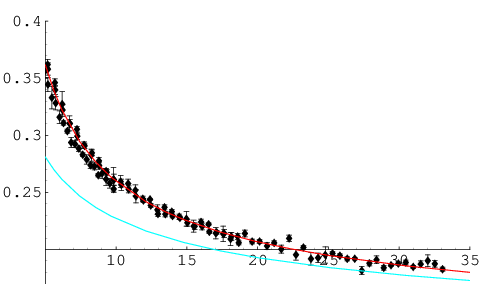 |
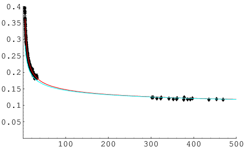 |
4 DSE numerical solutions
4.1 Solving the ghost propagator DSE
Let us analyze first in this section the general picture for the low-momentum Landau-gauge DSE solutions by applying the approach proposed for the first time in ref. [26]:to combine lattice gluon propagator results with a ghost propagator DSE truncated by a well supported hypothesis for the ghost-gluon vertex. The same procedure has been very recently followed for the analysis of the Coulomb-gauge DSE solutions in ref. [31] leading, as we shall discuss below, to a very analogous picture. It should be noted too that the authors of ref. [166] also successfully applied the same strategy of combining lattice data and DSE, in particular by invoking the lattice data for the truncation of the gap equation and studying the chiral symmetry breaking.
4.1.1 Landau gauge solutions
We shall present now the results of ref. [26] for the ghost solutions in Landau gauge. The goal was to see whether the two types of solutions ( and ) suggested by the previous analytical discussion in section 2 actually exist for the same gluon propagator input. A positive answer came out by solving numerically the ghost SD equation for given gluon propagator and vertex, as we shall briefly describe in the following. To this goal, we invoke again the renormalized DSE given by (19) and cast it into the appropriate subtracted form:
| (107) | |||||
where we work in the scheme, and set appearing in eq.(19) as the squared renormalisation scale ( has been chosen at an optimum GeV, not too high to allow the lattice data to be safe, and not too small in order that the differences between solutions at small momenta can be clearly displayed). An IR finite gluon propagator () extracted from lattice data in pure Yang-Mills theory, with Wilson gauge action, and a lattice volume equal to , is used for momenta lower than GeV ; this choice is justified to have moderate UV artefacts. This is then extended to larger momenta using a one loop asymptotic expansion (with GeV corresponding to the standard GeV of lattice quenched QCD). As for the ghost-gluon transverse form factor in Eq. (18), , it is taken to be constant with respect to both momenta 1616 16 This cannot be an exact statement, as already shown in perturbation by the calculations of ref. [4; 78] : although finite, the vertex invariants do depend on the momenta through the running . . As we said above, this is suggested by the lattice data for (i.e. for zero gluon momentum), but we extend it to all values of and . The authors of ref. [109] find a bare vertex very close to in this zero momentum gluon configuration for a large range of . Note that we have re-defined the coupling as in Eq. (107), which, as far as the constancy for the ghost-gluon transverse form factor is assumed, depends only on the renormalisation point chosen for the propagators; it is furthermore independent of the particular way used to define the renormalisation of the vertex. On the other hand, the redefined coupling can be also written in terms of bare quantities or related to the well-known running coupling in the Taylor scheme:
| (108) | |||||
where it should be remembered that , in MOM scheme. Eq. (107) can be still transformed to a new form which makes the numerical calculation and the presentation of the various solutions easier; for this, we subtract the equation at , to let the value of at the origin appear and to eliminate the reference to the particular renormalisation point , and we redefine also the unknown function to be calculated as . Then the reference to the value of also disappears; we end with :
| (109) | |||||
Equation Eq. (109) can be solved for , for a set of values of . It is easy to see that, from this, the desired solution of eq. (107) can be straightforwardly reconstructed for any renormalisation point and any value of . Indeed, as the MOM renormalization condition imposes , for any given and , we have just to identify the value of such that and reconstruct then through
| (110) |
By construction, all the solutions found in this way are finite at the origin and they correspond to the “decoupling” family of solutions that were described above in section 2. On the other hand, the solution which diverges at vanishing momentum appears as an end-point for the solutions of this “decoupling” family that can be approached by making larger and larger so as to get the limiting case: . Then, the critical “scaling” solution will be found by setting in eq. (109). As we will discuss below, this strategy for solving the DSE, after it had been followed in [26], was further applied by the authors of ref. [28] to the analysis of the coupled ghost and gluon DSE in Landau gauge, where they also concluded that the choice of amounted to fix a boundary condition for the DSE system and, consequently, to determine the class to which the actual solution belongs : either a “decoupling” one for any finite value of or the unique “scaling” one for . Unfortunately, the authors of ref. [28] missed the connection of and , and hence with the coupling at the renormalization point, , given by Eq. (110).
In ref. [26], the solutions of eq.(109) with the integral cut in the UV at GeV were obtained after discretization in and and solving by iteration1717 17 It should be noted that minus the integral in the r.h.s. is positive, allowing an easy convergence. We linearize it at each step, following the Newton method, to accelerate the convergence of the iteration procedure, as suggested by Bloch [68].. The results are the following:
1) Critical case, scaling solution: One finds a solution with , i.e. , the corresponding ”critical” constant being
| (111) |
The relation of eq.(46) for , obtained in sec. 2, should be verified by the numerical solutions and it happens to be very well satisfied:
| (112) |
The integration near can be improved by taking explicitly into account the analytical behavior of the kernel, and assuming that the solution behaves as at small . This imposes eq. (46), and one indeed can check that
| (113) |
although very slowly.
2) Regular case, decoupling solution: One finds a solution and only one for any with the method of solution described above. As can be seen below, a numerical solution at corresponds to the best description of lattice data (see Fig. 7, borrowed from ref. [26]). Furthermore, the asymptotic low-momentum behaviour for the ghost dressing function, giving a next-to-leading term, (cf. Eq. (2.1.5) ) is checked in ref. [26] (this is shown in Fig.6, also borrowed from this work) and the slope appears to agree pretty well with the prediction from Eq. (2.1.5): against .

The critical value of the coupling constant, as well as the corresponding curve of , can be very well approximated by the regular decoupling solutions at very large . When is larger and larger, Eq. (2.1.5) remains valid only in a smaller and smaller region near while, in an intermediate region, one observes the expected behaviour. In this way it is possible to show that, as long as the coupling constant does not exceed a critical value , where the scaling solution emerges (see also sec. 4.1.4 ), the solution goes to a constant in the infrared : one is in the decoupling case. As soon as the coupling constant reaches that critical value 1818 18 The existence and the value of this critical coupling had already been noticed, see for instance ref. [68]. the solution converts to the infrared-infinite one (“scaling situation”). Actually, the DSE solution accounted for the scaling solution when at the renormalization point GeV, as it is shown in Fig. 7. Admittedly, a real resolution of the DSE equations would require solving reciprocally the DSE for the gluon and verifying the compatibility of the solution with the gluon dressing function which was used as an input to build the kernel for the same g-value. We will deal with this below.
In conclusion, in the case , a continuum set of IR finite decoupling solutions for arbitrary emerges, and a unique singular scaling solution for , with , which appears to be the end-point for the previous ones.
4.1.2 Comparison with ghost lattice data
After the analytic study of the general solutions of the GPDSE in sec. 2 and the previous numerical analysis exhibiting both types of solutions for the ghost dressing functions, either regular (decoupling) or singular (scaling), the question also addressed in ref. [26] is: which one is effectively realised on the lattice, and therefore in true QCD?
A better means to provide us with an answer is offered by the numerical calculation in previous subsection that, predicting the behavior of the respective solutions for the ghost over the whole range of momentum, can be confronted to the lattice estimate for the ghost dressing function and that can lead us to identify which one offers the best agreement with the data 1919 19 At this stage, it is useful to stress the advantage of working with the renormalised form of the SD equations; indeed the continuum and lattice versions are more directly comparable than the bare ones. As the authors of ref. [24] have shown, the bare lattice equation for the ghost is affected by an important artefact which vanishes only very slowly with the cutoff, being of order . In the renormalised version, this effect is included in the renormalisation constant , and we are left only with the much smaller cutoff effects of the type .. This is done in ref. [26] and displayed here in fig. 7, where one can see that the singular scaling solution appears to be clearly discarded by the lattice data around and below GeV. On the contrary, a very good description of the lattice data in the range (clearly below the critical value) is found. This striking agreement, although for a narrow momentum window, is illustrated by Fig. 7 (As an indication, we quote the IR limit for the same and ).

An additional consistency test is obtained from using Eq. (108) to connect the continuum to the lattice bare quantities,
| (114) |
and then checking whether our range is reasonably consistent with the r.h.s. of eq.(114) as given by lattice data. In spite of the crude approximation made 2020 20 First, it is valid up to finite cutoff effects, as well as volume effects; second, we have replaced the lattice vertex invariant by the constant which, as we discussed above, is a rough approximation over the momenta which are actually implied in our calculation. In app. A, some non-perturbative corrections for this invariant, that appear to be pretty well in agreement with some SU(2) lattice estimates [165], will be discussed. to be left with Eq. (114), the result of the check is very encouraging: indeed, from the above value of found in the continuum on the one hand and the lattice data , and ( is here chosen as GeV) on the other, one finds to satisfy equation (114), which represents some kind of average on momenta. This number should be compared to the SU(3) lattice measurements which are performed at and have been submitted to a renormalization such that the result takes the value 1 at GeV, and which give about [109], with large errors.
Another striking way of presenting the difference between the regular decoupling solution and the singular scaling one is in terms of the familiar product, , which is proportional, at least for the UV domain, to the running coupling in Taylor scheme. This is shown in Fig. 8.

In ref. [105] new ghost propagator data are provided, coming from larger volume lattice simulations and covering a wider momentum range, with smaller momentum data, to compare with. The confrontation of those data with the results from the integration of the GPDSE truncated with the help of a lattice-based gluon propagator as done in sec. 4.1.1 requires, to account succesfully for the very low-momentum data, to go beyond the hypothesis of constancy of the ghost-gluon transverse form factor, . A possibility, studied in ref. [165] consists in applying an ansatz for the transverse form factor, , which is inspired by the OPE description for the non-perturbative corrections of the ghost-gluon vertex, obtained by applying the same procedure outlined in sec. 3.8 and by taking the gluon condensate value of table 4.
4.1.3 Coulomb gauge solutions
As we previously mentioned, the authors of ref. [31] recently performed a study (very analogous to the one in ref. [26] for Landau gauge) of the GPDSE in Coulomb gauge, obtained within the (second order) functional formalism, in order to investigate the low-momentum ghost dressing solutions. They took Gribov’s equal-time spatial gluon propagator dressing function 2121 21 In very good agreement with the Euclidean SU(2) lattice results obtained for small lattice couplings in ref. [168].,
| (115) |
as the input required to build a kernel and solve the GPDSE, again with the approximation of replacing the fully dressed spatial ghost-gluon vertex by the bare one (this is, also in Coulomb gauge, an exact result in the limit of a vanishing incoming ghost up to all perturbative orders [169]). Thus, the GPDSE is rewritten as follows:
| (116) |
where represents the angular integration,
| (117) |
It should be emphasized that the ghost propagator dressing function in Coulomb gauge is strictly independent of the energy, , as a non-perturbative consequence of the Slavnov-Taylor identities [170].
Assuming a pure powerlaw behaviour, , for the ghost dressing function and analyzing asymptotically Eq. (116), one is left in Coulomb gauge again with the two same cases we have encountered in Landau gauge: (i) (decoupling) and (ii) (scaling). As well in Landau as in Coulomb gauge, a massive gluon propagator generated via the Schwinger mechanism or Gribov’s fomula for the equal-time spatial dressing leads to and thus . In particular, from the next-to-leading analysis in sec. 2.2 of Eq. (24), one obtains [27] :
If , the perturbative strong coupling defined in the Taylor scheme [73], , goes to a non-zero constant at zero-momentum,
| (121) |
as can be obtained from Eqs. (64,4.1.3). In the case , the subleading correction to the non-zero finite value for the zero-momentum ghost dressing function, given by Eq. (4.1.3), is controlled by the well-defined zero-momentum limit of , which is the extension to the Taylor ghost-gluon coupling case [29] of the non-perturbative effective charge defined from the gluon propagator in ref. [74].
The same two cases result from the analysis of Eq. (116) for the Coulomb gauge in ref. [31], where a ghost propagator dressing function behaving asymptotically as either a constant or is analytically found and confirmed by a numerical study. This can be seen in the left plot of Fig. 9 which we borrowed from ref. [31]. In Coulomb gauge, the lattice results for the ghost propagator, within the available momentum window, may agree with decoupling and scaling solutions, and cannot help to discriminate.
It should be noted that the lagrangian approach to the Coulomb gauge (the continuum functional formalism is based on the QCD Lagrange density) is not the most widely used. However, and despite the technical difficulties mostly related to the inherent non-covariance of the Coulomb gauge, some recent progresses have been made in order to derive explicitely the DSE [169; 170; 171] (allowing the previous analysis) or studying the Bethe-Salpeter equation for heavy quarks [172]. The method which is most widely applied in the continuum is the canonical formalism based on the QCD Hamiltonian density operator [32; 173; 174; 175; 176]. Dyson-Schwinger-like equations (in a space with one less dimension) for the equal-time correlators are obtained in the canonical formalism and again the two types of solutions, critical and subcritical, are found for the propagator dressing function [32]. It seems to happen that, in the Coulomb-gauge canonical formalism, two different values for the infrared exponents emerge in the critical case and that the favoured one is the one which produces the most singular ghost dressing, which diverges as in the infrared, i.e. similarly to the critical solution discussed above (with ).
 |
 |
4.1.4 The critical limit of decoupling solutions from the GPDSE analysis
In summary, the GPDSE in Eq. (24) with the input of a gluon propagator borrowed from lattice QCD calculations can be numerically solved and two kinds of solutions result and appear to be controlled by the size of the coupling at the renormalization point 2222 22 In QCD, one needs to provide a physical scale and a standard manner to proceed is by fixing the size of the coupling at a given momentum scale. This can be seen as a boundary condition to solve the DSEs., . For any coupling below some critical value, , an infinite number of regular or decoupling solutions for the ghost dressing, behaving as Eq. (4.1.3) indicates, are found; for , a unique critical or scaling solution behaving as Eq. (4.1.3) is found, and no other type of solutions appears to exist. In ref. [26], for a subtraction point GeV, a critical coupling and a very good description of ghost propagator lattice data with a regular solution of Eq. (24) for were obtained.
As we shall discuss in the next section, these results were also recently confirmed [177] by studying the coupled system of ghost and gluon propagator DSE in the PT-BFM scheme [178]. This last work paid attention to the critical solution limit by studying how diverges as , with a subtraction point GeV. In addition, the author of ref. [154] applied the perturbative definition of the Taylor strong coupling in Eq. (121) to compute this coupling with the gluon and ghost solutions of [177] in order to see how the critical limit is approached. This is shown by the right plot of Fig. 9, borrowed from ref. [154], where it can be also seen that all the curves for obtained for different values of tend to superpose over each other as increases (right). As a striking check of consistency, the curve for the critical limit in this right plot of Fig. 9 is obtained by rescaling, up to giving from Eq. (121) with at zero-momentum, the results at the critical limit for numerically obtained in ref. [26] and plotted here in Fig. 8 of the previous subsection. Indeed, the critical value for the coupling at GeV can be read from the critical curve in Fig. 9 and one gets , in fairly good agreement with the value of ref. [177].
On the other hand, the numerical analysis of Eq. (116) for the Coulomb gauge in ref. [31] also shows both the regular and the critical solutions to exist, but being controlled by (or ) as a boundary condition with the size of the coupling fixed to be for (see the right plot of Fig. 9). Regular or decoupling solutions appear for finite values of and critical or scaling solution for . Nevertheless, the authors of ref. [31] concluded that, as far as all the solutions join each other in the perturbative domain (see the right plot of Fig. 9) and can be found for a fixed coupling, the boundary condition is not connected to the renormalization and claimed for a contradiction with the Landau-gauge results of ref. [26].
Finally, the two pictures for the low-momentum solutions from GPDSE, either a family of Landau-gauge DSE solutions labelled by the size of the coupling at the renormalization point or a family of Coulomb-gauge ones labelled by the zero-momentum ghost dressing value as a boundary condition independent of the renormalization, were reconciled by the work of ref. [154]. The key point stems from the different renormalization prescriptions applied to the ghost propagator in both analyses. MOM scheme in the Landau-gauge analysis of refs. [26; 27; 177], and the prescription applied to the ghost propagator in eq. (3.20) of ref. [31] for the renormalization constant , where . In particular, this last renormalization constant depends on the boundary condition, , in such a manner that the value for this boundary condition is rescaling the ghost dressing function (and, as can be clearly seen in Fig. 2 of [31], it does not take the tree-level value, 1, as happens in MOM prescription for the subtraction point). Thus, according to ref. [154], the non-trivial connection between solutions in both schemes, that relies on the relation previously shown by Eq. (110), comes out from the following property of Eqs. (24,116): let be a MOM solution of Eq. (24) for arbitrary coupling, ; if we then apply the following transformation:
| (122) |
for any c-number , the transformed dressing function verifies the DSE equation with the transformed coupling (of course, MOM prescription implies ). Then, one only needs to choose and to apply the transformation to every solution of the MOM family and one will be left with a one-to-one correspondence between these solutions and the new ones
| (123) |
for the fixed coupling , which can be identified by the zero-momentum value, . This new family of transformed solutions obeys the same pattern as the Coulomb gauge family in ref. [31] and corresponds, up to the fixed number (which does not even depend on the renormalization point), to the family of solutions obtained by the analysis for Landau gauge in previous sec. 4.1.1. It is interesting to note that the strong coupling defined in the Taylor scheme can be also obtained from the transformed solutions as
| (124) |
although it is obvious that neither nor the coupling are in MOM scheme.
Thus, the same picture for the low-momentum Green function solutions emerges in both Landau and Coulomb gauge from the analysis of the GPDSE: a family of MOM-renormalized regular decoupling solutions, characterised by the value of the coupling at the renormalization point; and a singular scaling solution as an end-point for the family of regular ones. An interesting final remark is that the input parameter for the solutions in ref. [31], the zero-momentum ghost dressing, can be put in connection with the Gribov problem [31]; while, for Landau gauge and MOM scheme, is related to the strong coupling in Taylor scheme, as was shown in Eq. (108). This is not the case for the size of the fixed coupling, , after applying Eq. (122) which is physically meaningless.
4.2 The ghost and gluon propagator coupled DSEs
Satisfying the GPDSE, as was required in sec. 2, is a necessary but not sufficient condition for a DSE solution to exist. Of course, the existence of a solution can only be confirmed by treating the infinite tower of DSEs, but this is an impossible task. In the previous section, sec. 4.1, this infinite tower of DSEs was truncated by plugging into the one among them to be solved, the GPDSE in that case, the available lattice data, or a model compatible with them, for the gluon propagator and the ghost-gluon vertex. On the other hand, the usual approach consists in applying a truncation scheme based on hypotheses and approximations that preserve the main properties of the theory and that leave us with a closed system of equations to deal with. The former approach can be seen to provide with a consistency analysis of the lattice and DSE picture for the solutions and benefits of not “polluting” the conclusions with the possible implications of any particular truncation scheme. However, the DSE picture should be completed by also applying the latter usual approach.
As we shall discuss below, both scaling and decoupling solutions have also been proven to emerge when the DSEs are truncated so as to give a coupled system for the ghost and gluon propagators.
4.2.1 Scaling solutions
As we have repeated insistantly in this paper, it has been recognized for a long time that the set of solutions of the DSEs for the ghost and gluon propagators consists in a continuum of so-called “decoupling” solutions augmented with a unique “scaling” one (cf. ref. [66]); which one is actually encountered depends on the value of the coupling constant. Nevertheless, for quite a time, attention has mainly be paid to the scaling one which, in practice, was obtained by replacing the fully dressed vertices by ansätze which take into account as much information as possible (see ref. [15] for a first review on the subject). The loops in DSEs had been proven to be dominated by the infrared contributions for the scaling solution [108; 179] which had been fully worked-out in ref. [66] (see also ref. [59]). The infrared exponents for the power behaviour on the momentum for both ghost and gluon dressing functions being related by , the value for one of them, usually the one for the ghost, , completely characterizes the low-momentum solution. Under the assumption of a constant ghost-gluon transverse form factor, the only solution to emerge in the interval ( [66]) is , as was numerically put forward by the authors of ref. [180], and independently confirmed by the analysis performed in ref. [50] with the help of renormalization group methods (RGE). Then, the uniqueness of the the above-mentioned low-momentum solution defined by was discussed in two papers [30; 52], first (wrongly) claimed to be true in general for the coupled DSE system [30] and later on concluded to happen only for scaling-type solutions [52], i.e. provided that the relation is “a priori” assumed (we will pay attention to this in a next subsection).
Very recently, the authors of ref. [28] re-analysed the problem of the low-momentum properties of the Yang-Mills Green functions by following both DSEs and RGE approaches and found both scaling and decoupling solutions to exist. They paid special attention to the truncation schemes and also claimed that only the (unique) scaling solution satisfies BRST invariance, while the decoupling ones would be at odds with it. This was presented as an incitation to prefer the scaling solution as the “real” QCD one but, as was previously mentioned when discussing the Gribov-copies problem, Gribov or Gribov-Zwanziger (either refined or not) approaches to avoid the copies already imply a BRST breaking and this only prevents the Kugo-Ojima confinement scenario from working. Other confinement scenarios are of course possible and nothing indeed prevents the decoupling solution from being, as lattice appears to indicate, the real QCD one.
The properties and implications of the scaling-type low-momentum solutions have been extensively discussed in the literature. We address the interested reader to reviews like the ones in ref. [15; 68; 167] as well as to the numerous works qoted above or to others like ref. [181] focusing on the Kugo-Ojima criterium implications, refs. [175; 182; 183] on the infrared behaviour of vertices, ref. [81] on the analysis of infrared sigularities or ref. [184] about the study of scaling solutions in the maximally abelian gauge.
We will now end this section by adding a few words about the elusiveness of decoupling solutions, after the scaling one has been proposed.
4.2.2 Why have the decoupling solutions been so elusive?
The decoupling or regular solutions have been missed for almost ten years. Why? they could not have been previously obtained by the proponents of the relation (Rel) because, as it seems to us, they discarded them from the very beginning, and thereby chose the critical value of the coupling constant, by making an implicit assumption when solving the so-called “infrared equation” for the ghost SD equation. This can be seen, for instance, in ref. [179], eqs. (43) and (44), or in the detailed discussion of Bloch [68]), eqs. (55) to (58).
Let us explain this briefly. They consider the above unsubtracted equation (note that this requires then an UV cutoff, which we avoid in our previous analysis by considering the subtracted form); we write again the unsubtracted form:
| (125) |
One must try to match the small behaviour of the two sides of Eq. (125). This is done for example in eq. (58) of [68]. A condition is then written which consists in equating the coefficient of with the corresponding one in the r.h.s.. However, one notices that on the r.h.s., there is a constant contribution . Therefore unless the constant term is cancelled by the integral contribution for , we have necessarily . To have as the author finds, one needs this cancellation. This is what is implicitly assumed, but not stated explicitly. The condition of cancellation is :
| (126) |
However, this additional equation does not derive from the starting SD ghost equation, and indeed it is not satisfied in general by the solutions of this basic equation, as we show by displaying actually IR finite solutions. In fact, it can be valid only for a particular value of the coupling constant, the critical one which is solution to the equation of Bloch, his eq. (58), and which we derive rigorously through the subtracted equation. A similar conclusion is obtained in the analysis of ref. [28], although its authors missed the connection between their boundary condition, the zero-momentum value of the renormalized ghost dressing function, and the coupling size at the renormalization momentum.
4.2.3 Decoupling or massive solutions
A decoupling behaviour has also been proven to result as a solution of a coupled system of gluon and ghost propagators DSEs. First, the authors of ref. [185] implemented some ansätze based on Slavnov-Taylor identities for the involved full vertices, applied a particular angular approximation when integrating the ghost self-energy and thus obtained a “massive” gluon propagator (), although they claimed this to be compatible with an enhanced ghost propagator. Then, as mentioned above, the Schwinger mechanism of mass generation [69] was proven to be consistently incorporated into the gluon propagator DSE through the fully-dressed non-perturbative three-gluon vertex and to give rise to the generation of a dynamical gluon mass [70; 19]. Then, a massive solution for the coupled ghost and gluon propagator DSE was shown to apppear [71] in the PT-BFM truncation scheme (see also [186]). The lattice data result to be furthermore very well accommodated within coupled DSEs in the PT-BFM scheme [20]. As a matter of fact, as will be seen below, the PT-BFM DSEs solutions have been shown to asymptotically behave as Eqs.(64, 69) predict for a decoupling solution [177]. The authors of ref. [28] also confirmed the decoupling solutions to be present by the analysis of the coupled DSEs and the functional Renormalization group equations (FRGs). They also obtained an infinite family of decoupling solutions, as was discussed in sec. 4.1.4 but they used the zero-momentum ghost propagator as the boundary condition for the DSEs integration and missed its connection with the value of the coupling at the renormalization momentum (i.e. the particular value of one applies to build the solutions) or the critical coupling the scaling behaviour requires to emerge. This connection is an important ingredient because it provides us with a manner, through a comparison with the physical strong coupling, to discuss whether the scaling critical DSE solution could be allowed by the data.
We will now present, in the following, the comparison performed in ref. [177] of the decoupling analytical low-momentum expressions, given here by eqs. (64,69), and the PT-BFM solutions shown to provide a quantitative description of lattice data [20; 187]. The main feature in the PT-BFM scheme is that it guarantees the transversality of the gluon self-energy order-by-order in the dressed-loop expansion, thus leading to a gauge-invariant truncation of the gluon DSE [186]. In this PT-BFM scheme for the coupled DSE system, the ghost propagator DSE is the same as the one given by eqs. (24), where the bare ghost-gluon vertex is approximated by . The gluon DSE is given by
| (127) |
where
| (128) |
In the diagrams of (128) for the gluon DSE, Eq. (127), the external gluons are treated, from the point of view of Feynman rules, as background fields (these diagrams should be also properly regularized, as explained in [178]). This is what justifies the four field coupling of two background gluons and two ghosts leading to the contribution . The function is defined in ref. [188] through a so-called background quantum identity [178] and can be, in virtue of the ghost propagator DSE, connected to the ghost propagator [29; 187]. The coupled system is to be solved, by numerical integration, with the two following boundary conditions as the only required inputs: the zero-momentum value of the gluon propagator and that of the coupling at a given perturbative momentum, GeV in this particular case, that will be used as the renormalization point. This is done by varying the boundary conditions (In particular, as explained in ref. [177], by keeping the zero-momentum value of the gluon propagator fixed while is ranging from 0.15 to 0.1817) and leaves us with a family of massive or decoupling solutions that eqs. (64,69) must account for, in the low-momentum domain. The successful confrontation can be seen in Fig. 1 of [177], from which we extract, as an example, the plot in Fig. 10.
 |
 |
The ghost dressing function at vanishing momentum, , is also shown to diverge as , by obeying a power behaviour, s
| (129) |
where the coefficient is a positive critical exponent (depending presumably on the renormalization point, ) which governs the transition from decoupling () to the scaling () solutions. This is seen in Fig. 2 of ref. [177] and confirms the results from the GPDSE analysis in sec. 4.1.4.
Had one let be a free parameter to be fitted by requiring the best linear correlation for in terms of , one would have obtained a best correlation coefficient of 0.9997 for and (which is pretty close to the critical value of the coupling above which the coupled DSE system does not converge any more). This last critical value at GeV for the coupling can be pretty well translated to that of in (see for instance eqs.(22,23) of ref. [73]) and then compared to in pure Yang-Mills from the lattice 2323 23 It should be noted that the procedures for the lattice determination of mainly work in the UV domain, where IR sources of uncertainties as the Gribov ambiguity or volume effects are indeed negligible. In fact, there are unquenched lattice determinations with staggered fermions for the strong coupling [189] which are pretty consistent with the PDG value.. The latter is estimated to be 238(19) MeV [190], clearly below the former, 434 MeV, for the critical limit for the PT-BFM DSE in pure Yang-Mills.
In summary, one can clearly conclude that the analysis of the coupled DSEs also agrees with the existence of both decoupling and scaling classes of solutions and with the pattern for them described in sec. 4.1.4. In particular, the analysis of the solutions in the PT-BFM scheme proved the scaling one to appear as an end-point for the decoupling family in Landau gauge, when the coupling at the renormalization point approaches a critical value. This critical value, at GeV, is well above the lattice estimates for the coupling, in total consistence with the conclusion of lattice QCD favouring the decoupling solution presented in sec. 3.
Of course, gluon and ghost propagators and the vertices involving them, altogether with quark propagators and the quark-gluon vertex, are basic building blocks to study the QCD bound states. It might be that the exact very low-momentum behaviour of gluon and ghost propagators, that we paid attention to, is not very relevant for much of the hadron physics. In particular, the quark functions can be studied by modelling the product of the dressed gluon propagator and the quark-gluon vertex and, regardless of whether the gluon is suppressed or massive, the key region for physics is the momentum region of [191; 192]. Nevertheless, the dressed quark propagator, using massive gluons with non-singular interaction in the quark-gluon vertex, do become like expected by the heavy quark effective theory [65]. Furthermore, many phenomenological works also appear to support a massive gluon solution, as can be seen in the review of ref. [178], and references therein, or, as very recent examples, in the works of refs. [193; 194; 195; 196]. This also favours a decoupling solution.
5 Conclusions
With this paper, we aimed to give an overview for the current state-of-the-art concerning the infrared properties of pure Yang-Mills QCD Green functions. Very much work has been reported in the last few years, modifying essentially the paradigm about this subject and demanding some sort of update for past reviews that can be found in literature. About ten years ago, the results from Landau gauge DSEs and FRGs analysis agreed with a solution, now dubbed “scaling”, where the low-momentum behaviour for the two-point correlators appears to be an enhanced ghost propagator and a vanishing gluon propagator at zero-momentum ( and , according to the notation of Eq. (6)). At that time, the lattice estimates for both correlators resulted to be compatible with this low-momentum behaviour, other approaches like the ones applying stochastic quantization methods and Gribov-Zwanziger lagrangian also pointed to the same results and all together matched the Kugo-Ojima confinement criterion providing a framework for the infrared solutions of Yang-Mills Green functions that was generally accepted. However, more recent results for the two-point correlators with larger lattices, some of them paying special attention to the problem of Gribov’s copies, seemed to establish a different pattern for the low-momentum solutions: a finite ghost dressing and a finite non-zero gluon propagator at zero-momentum ( and ), which did not agree with the scaling behaviour that would require the ghost and the gluon infrared exponents to be related by . On the other hand, other authors, applying a particular truncation scheme for the gluon propagator DSE which involves some angular approximation for the momentum integration, proposed a massive gluon propagator (), consistently with the PT gluon propagator. Then, the GPDSE was recently re-analysed by exploiting the interplay of DSEs and lattice results and, apart from the scaling solution, new ones with , now dubbed decoupling, were proven to exist, which do not observe the scaling behaviour but are totally compatible with lattice results. Thus, both scaling and decoupling solutions have been now proven to emerge as solutions of the coupled system of gluon and ghost propagators DSEs for different truncation schemes, such as for instance the PT-BFM. The same occurs for FRGs.
On the other hand, we have reviewed the plethora of lattice works on the subject, also discussing with some detail the role and impact of the lattice artefacts, and concluded that the current paradigm is a massive gluon and a free ghost, i.e. a decoupling low-momentum behaviour for the two-point Green functions. Apart from the lattice results, the application of some refinement of the Gribov-Zwanziger approach and other new approaches also appear now to agree with a decoupling behaviour for the low-momentum Green functions solutions. When solving the DSEs, the solutions have been proven to be “dialed” by the size of the coupling at the renormalization point, which can be univocally related to the zero-momentum value of the renormalized ghost dressing function. A family of decoupling solutions corresponds to a family of sub-critical ones for finite values of the zero-momentum ghost dressing and for any coupling below a critical value at the renormalization point. As for the scaling solution, it can be considered as “critical”, since it emerges for a unique (critical) value of the coupling for which the ghost dressing diverges at zero-momentum. A very similar pattern is shown to happen for the equal-time spatial gluon propagator and the ghost dressing function in Coulomb gauge.
Of course, the critical value of the coupling depends on the renormalization point but, once it is known for one particular momentum, this value can be propagated to any other by applying the definition of the Taylor coupling in Eq. (5) and the scaling solutions for ghost and gluon dressing functions. This is of course a consequence of the renormalization scaling for the coupling definition, which does not depend on either the cut-off, when written in terms of bare quantities, or the renormalization point, when expressed with renormalized ones. The critical value obtained at 10 GeV in the PT-BFM scheme, in agreement with the analysis of the GPDSE with a lattice gluon propagator as input, is shown to be definitely above the lattice estimate for the Yang-Mills Taylor coupling, favouring again a decoupling solution in Landau gauge.
The truncation of the tower of DSEs which is necessary to obtain a (finite) tractable system of equations implies approximating the vertices. In particular, the ghost-gluon vertex plays a crucial role in the analysis which led to find out the decoupling solutions, but also the three-gluon vertex is an essential ingredient for the gluon propagator DSE in any scheme. The ghost-gluon vertex benefits of Taylor’s theorem that has been revised in the appendix, where we also discussed which OPE non-perturbative corrections to the vertex the dimension-two gluon condensate induces. For the sake of consistency, we also overviewed the results from many lattice investigations about the impact of these OPE corrections on the Yang-Mills Green functions and about the possibilities of determining the size of the gluon condensate. Concerning the vertices, although some works have been devoted to investigate their properties, more lattice and continuum investigations would be very welcome.
To summarize, in the current state-of-the-art, although both types of solutions are compatible with DSEs (and FRGs too), lattice QCD and some continuum approaches, like mainly RGZ, seem to favour a decoupling-type of solutions which implies a free ghost and a massive gluon.
Acknowledgements.
We thank M. Müller-Preussker and A. Sternbeck for very valuable comments and for providing us with some material to be published. One of us (J. R-Q) is also indebted to D. Dudal for very fruitful discussions and comments. This work has been partially supported by the research projects FPA2009-10773 form the Spanish MICINN and by P07FQM-02962 from “Junta de Andalucía”.Appendix A A main ingredient: the non-renormalization Taylor’s theorem
A.1 What does the Taylor’s theorem indeed say?
A widely used statement, known as the “non-renormalization theorem”, claims that, in the Landau gauge, the renormalization constant of the ghost gluon vertex is exactly one. Note that there is no reference to a particular renormalisation scheme. Formulated in this way, this claim is wrong. Let us first state and then explain below what is true in our opinion :
1) There is a true and very clear statement which can be extracted from Taylor’s paper (the argument is given below), ref. [75].
| (130) |
i.e. there is no radiative correction in this particular momentum configuration (with zero momentum of the ingoing ghost)
2) This entails that is finite whatever the external momenta, and that therefore . In addition, we get also trivially , where MOMh refers to the configuration of momenta in equation (130). In general, in other schemes, there is a finite renormalisation, and this is why one must be very careful when using the misleading expression: ”non-renormalization”.
3) In particular, one finds in the very extensive calculations of radiative corrections at least two cases of MOM schemes where there is a finite renormalisation (and certainly many more) : MOMg in the notations of ref.[4], and the symmetric MOM scheme. For the latter, we give the proof below.
The essence of Taylor’s argument is actually very simple. In a kinematical situation where the incoming ghost momentum is zero, consider any perturbative contribution to the ghost-gluon vertex. Following the ghost line in the direction of the flow, the first vertex will be proportional to the outgoing ghost momentum , i.e. to the gluon momentum . In the Landau gauge this contribution will thus give 0 upon contraction with the gluon propagator. Therefore the only contribution to remain is the tree-level one. In other words the bare ghost-gluon vertex is shown to be equal to its tree-level value in these kinematics : . This result has been checked by means of a direct evaluation to three loops in perturbation theory by Chetyrkin. In our notations :
| (131) |
Note that in the Schwinger-Dyson equation (19), only is present, and the theorem by Taylor does not tell that , as seems assumed in many Schwinger-Dyson calculations.

As an illustration of our point 3), let us quote the formulas from the appendix of ref. [4], reduced to the situation we are interested in (). The two dressing functions (resp. ) are defined by (resp. ) and correspond to the kinematical situations depicted in the left (resp. right) part of fig. (11). We have already mentioned that is exactly one, but this does not hold for and, indeed, one has at three loops :
| (132) | |||||
It is then easy to find the -dependence :
In ref. [66] the non-renormalization theorem is understood as the statement that the vertex reduces to its tree-level form at all symmetric-momenta points in a symmetric subtraction scheme. However this statement is not supported by a direct evaluation. Using the one-loop results of Davydychev (ref. [78]) one gets in a symmetric configuration the value
| (133) |
with .
According to ref. [66] the coefficient of should be one. The presence of in the above formulas implies on the contrary that the vertex will in general depend on the momenta : using the results given in the appendices of ref.[4] one finds for the leading -dependence
This dependence is logarithmic, as is expected in a perturbative approach. Furthermore, in ref. ([66]) it is supposed that the vertex function takes the form with the restriction . This restriction comes from the assumption that the symmetric vertex is equal to 1 for any , which, as we have just seen, is actually not the case. Therefore, it should be necessary to adopt a more general point of view and keep open the possibility of a non perturbative effect on . We should mention that, actually, the problem of the -dependence of the ghost-gluon vertex has already been addressed in refs. [182; 183]. However these authors work under the condition which appears not to be satisfied by lattice data. Also in ref. [165], the impact of the OPE non-perturbative corrections, as the one we dealt with in sec. 3.8, is studied for the ghost-gluon vertex in order to go beyond the approximation of taking the Taylor kinematics for the transverse form factor. We will briefly pay attention to this in the next subsection.
A.2 Non-perturbative corrections for the ghost-gluon vertex
The non-perturbative effect resulting from a non-zero in a OPE expansion, shown in sec. 3.8 to have non-negligeable effects on ghost and gluon propagators at energies of the order of 2-3 GeV and still visible at around 7 GeV, can be also advocated to have an impact on the ghost-gluon form factors introduced in Eq. (18), in particular on the transverse form factor, , needed for the integration of the GPDSE in sec. 4.1. The procedure outlined in sec. 3.8 is also in order to compute the Wilson coefficients for such a non-perturbative contributions. Then, Eq. (101) can be particularized to be
| (134) |
| (a) | (b) |
where, although it is not divergent, one can apply a finite renormalization to require to take its tree-level value, , at a given momentum scale, , for a particular kinematical configuration of and (for instance, ). This dependence on should be understood for the Wilson coefficient and the form factors. The Wilson coefficient can be obtained [165] at tree-level by evaluating the diagrams in Fig. 12 and reads:
| (135) |
Thus, after modeling the ghost-gluon form factor all over the range of their momenta by the insertion of some infrared mass scale to saturate the powers of momenta in the denominators of Eqs. (135) (as a simple way to avoid the non-physical divergence coming from these inverse powers), one obtains the model for the ghost-gluon transverse form factor that was mentioned in sec. 4.1.2. This model provides us with a first correction to the usual hypothesis for the GPDSE integration: that is encoded by the OPE expansion through .
It is interesting to notice that, had we considered the kinematic configuration for the Taylor scheme, , one would obtain a non-vanishing OPE power correction for the transverse form factor; although no deviation from the Taylor result shown by Eq. (131) would result, because
| (136) |
as it is proved in ref. [165].
Appendix B The Dyson-Schwinger equation as a Ward-Slavnov-Taylor identity
A very general method to derive Slavnov-Taylor identities consists in taking advantage of the transformation properties of
| (137) |
under gauge transformations (cf. [76]).
is the Faddeev-Popov operator and the notation , indicates that the source term has to be kept, although it will eventually be set to 0 (this is denoted in the following by the suppression of the subscript). Taking the derivative of the gauge transformed of eq. (137) with respect to the gauge parameters leads to the general Slavnov-Taylor equation
| (138) |
is the ghost propagator and its presence here is simply due to its very definition as the inverse of the Faddeev-Popov operator. If one derives eq. (138) with respect to one gets :
| (139) | |||||
A first consequence of this relation is the triviality of the longitudinal gluon propagator. To see this, it suffices to derive both its sides with respect to and to set to zero. The result is
| (140) | |||||
In order to derive the second line we have invoked the fact that , the Faddeev-Popov operator, is the inverse of the ghost propagator . Thus, in momentum space, the general form of the gluon propagator for an arbitrary covariant gauge reads
| (141) |
Turning now back to eq. (139) and letting go to zero we obtain
| (142) |
which is nothing else than the GPDSE. Actually its l.h.s. involves only the longitudinal part of the gluon propagator, that we have just seen to be trivial :
| (143) |
where the symbol stands as usual for the d’Alembertian. As for the r.h.s it can be rewritten as :
| (144) |
The 3-point gluon-ghost Green’s function can be expressed in terms of vertex functions and propagators through
| (145) | |||
Now, we Fourier-transform Eq. (142), use eqs. (143-145) and obtain
| (146) | |||||
where the usual form of GPDSE can be recovered from by multiplying with and dividing by , which leads to
| (147) | |||||
This is a general result, valid in any covariant gauge. Of course the -depending (longitudinal) term disappears in Landau gauge. is related to the quantity, , that was previously introduced in section 1 through
and it is usually decomposed into . After inserting this in eq.(147) and restricting to the Landau gauge case one finally obtains
| (148) |
References
- [1] Kenneth G. Wilson. CONFINEMENT OF QUARKS. Phys. Rev., D10:2445–2459, 1974.
- [2] John M. Cornwall. Quark Confinement and Vortices in Massive Gauge Invariant QCD. Nucl.Phys., B157:392, 1979.
- [3] Jeff Greensite. An introduction to the confinement problem. Lect.Notes Phys., 821:1–211, 2011.
- [4] K.G. Chetyrkin and A. Retey. Three loop three linear vertices and four loop similar to MOM functions in massless QCD. hep-ph/0007088, 2000.
- [5] B. Sheikholeslami and R. Wohlert. Improved Continuum Limit Lattice Action for QCD with Wilson Fermions. Nucl.Phys., B259:572, 1985.
- [6] Y. Iwasaki and T. Yoshie. Renormalization Group Improved Action for SU(3) Lattice Gauge Theory and the String Tension. Phys.Lett., B143:449, 1984.
- [7] M. Luscher and P. Weisz. On-Shell Improved Lattice Gauge Theories. Commun.Math.Phys., 97:59, 1985.
- [8] M. Luscher and P. Weisz. Computation of the Action for On-Shell Improved Lattice Gauge Theories at Weak Coupling. Phys.Lett., B158:250, 1985.
- [9] Patrick O. Bowman, Urs M. Heller, Derek B. Leinweber, Maria B. Parappilly, and Anthony G. Williams. Unquenched gluon propagator in Landau gauge. Phys. Rev., D70:034509, 2004.
- [10] Patrick O. Bowman, Urs M. Heller, Derek B. Leinweber, Maria B. Parappilly, Anthony G. Williams, et al. Unquenched quark propagator in Landau gauge. Phys.Rev., D71:054507, 2005.
- [11] Maria B. Parappilly, Patrick O. Bowman, Urs M. Heller, Derek B Leinweber, Anthony G. Williams, et al. Effects of dynamical sea-quarks on quark and gluon propagators. AIP Conf.Proc., 842:237–239, 2006.
- [12] Paulo J. Silva and Orlando Oliveira. Unquenching the Landau Gauge Lattice Propagators and the Gribov Problem. PoS, LATTICE2010:287, 2010.
- [13] F.J. Dyson. The S matrix in quantum electrodynamics. Phys.Rev., 75:1736–1755, 1949.
- [14] Julian S. Schwinger. On the Green’s functions of quantized fields. 1. Proc.Nat.Acad.Sci., 37:452–455, 1951.
- [15] Reinhard Alkofer and Lorenz von Smekal. The Infrared behavior of QCD Green’s functions: Confinement dynamical symmetry breaking, and hadrons as relativistic bound states. Phys.Rept., 353:281, 2001.
- [16] S. Mandelstam. Approximation Scheme for QCD. Phys.Rev., D20:3223, 1979.
- [17] S. Mandelstam. General Introduction to Confinement. Phys.Rept., 67:109, 1980.
- [18] Nicholas Brown and M.R. Pennington. Studies of Confinement: How the Gluon Propagates. Phys.Rev., D39:2723, 1989.
- [19] Arlene C. Aguilar and Joannis Papavassiliou. Gluon mass generation in the PT-BFM scheme. JHEP, 0612:012, 2006.
- [20] A. C. Aguilar, D. Binosi, and J. Papavassiliou. Gluon and ghost propagators in the Landau gauge: Deriving lattice results from Schwinger-Dyson equations. Phys. Rev., D78:025010, 2008.
- [21] Attilio Cucchieri and Tereza Mendes. What’s up with IR gluon and ghost propagators in Landau gauge? A puzzling answer from huge lattices. PoS, LAT2007:297, 2007.
- [22] I.L. Bogolubsky, E.M. Ilgenfritz, M. Muller-Preussker, and A. Sternbeck. The Landau gauge gluon and ghost propagators in 4D SU(3) gluodynamics in large lattice volumes. PoS, LAT2007:290, 2007.
- [23] A. Sternbeck, E.-M. Ilgenfritz, M. Muller-Preussker, and A. Schiller. The Gluon and ghost propagator and the influence of Gribov copies. Nucl.Phys.Proc.Suppl., 140:653–655, 2005.
- [24] Philippe Boucaud, J.P. Leroy, A. Le Yaouanc, A.Y. Lokhov, J. Micheli, et al. The Infrared behaviour of the pure Yang-Mills green functions. hep-ph/0507104, 205
- [25] A. Sternbeck, L. von Smekal, D. B. Leinweber, and A. G. Williams. Comparing SU(2) to SU(3) gluodynamics on large lattices. PoS, LAT2007:340, 2007.
- [26] Philippe Boucaud, J-P. Leroy, A.Le Yaouanc, J. Micheli, O. Pène, et al. IR finiteness of the ghost dressing function from numerical resolution of the ghost SD equation. JHEP, 0806:012, 2008.
- [27] Philippe Boucaud, J.P. Leroy, A. Le Yaouanc, J. Micheli, O. Pène, et al. On the IR behaviour of the Landau-gauge ghost propagator. JHEP, 0806:099, 2008.
- [28] Christian S. Fischer, Axel Maas, and Jan M. Pawlowski. On the infrared behavior of Landau gauge Yang-Mills theory. Annals Phys., 324:2408–2437, 2009.
- [29] A. C. Aguilar, D. Binosi, J. Papavassiliou, and J. Rodriguez-Quintero. Non-perturbative comparison of QCD effective charges. Phys. Rev., D80:085018, 2009.
- [30] Christian S. Fischer and Jan M. Pawlowski. Uniqueness of infrared asymptotics in Landau gauge Yang-Mills theory. Phys.Rev., D75:025012, 2007.
- [31] Peter Watson and Hugo Reinhardt. The Coulomb gauge ghost Dyson-Schwinger equation. Phys.Rev., D82:125010, 2010.
- [32] D. Epple, H. Reinhardt, W. Schleifenbaum, and A.P. Szczepaniak. Subcritical solution of the Yang-Mills Schroedinger equation in the Coulomb gauge. Phys.Rev., D77:085007, 2008.
- [33] Markus Leder, Jan M. Pawlowski, Hugo Reinhardt, and Axel Weber. Hamiltonian Flow in Coulomb Gauge Yang-Mills Theory. Phys.Rev., D83:025010, 2011.
- [34] John M. Cornwall. Positivity issues for the pinch-technique gluon propagator and their resolution. Phys.Rev., D80:096001, 2009.
- [35] Ph. Boucaud, M.E. Gomez, J.P. Leroy, A. Le Yaouanc, J. Micheli, et al. The low-momentum ghost dressing function and the gluon mass. Phys.Rev., D82:054007, 2010.
- [36] V.N. Gribov. Quantization of Nonabelian Gauge Theories. Nucl.Phys., B139:1, 1978.
- [37] G. Dell’Antonio and D. Zwanziger. Every gauge orbit passes inside the Gribov horizon. Commun.Math.Phys., 138:291–299, 1991.
- [38] Daniel Zwanziger. Action from the Gribov horizon. Nucl.Phys., B321:591, 1989.
- [39] Daniel Zwanziger. Renormalizability of the critical limit of lattice gauge theory by BRS invariance. Nucl.Phys., B399:477–513, 1993.
- [40] Kei-Ichi Kondo. Kugo-Ojima color confinement criterion and Gribov-Zwanziger horizon condition. Phys.Lett., B678:322–330, 2009.
- [41] D. Dudal, R.F. Sobreiro, S.P. Sorella, and H. Verschelde. The Gribov parameter and the dimension two gluon condensate in Euclidean Yang-Mills theories in the Landau gauge. Phys.Rev., D72:014016, 2005.
- [42] D. Dudal, S.P. Sorella, N. Vandersickel, and H. Verschelde. New features of the gluon and ghost propagator in the infrared region from the Gribov-Zwanziger approach. Phys.Rev., D77:071501, 2008.
- [43] David Dudal, John A. Gracey, Silvio Paolo Sorella, Nele Vandersickel, and Henri Verschelde. A Refinement of the Gribov-Zwanziger approach in the Landau gauge: Infrared propagators in harmony with the lattice results. Phys.Rev., D78:065047, 2008.
- [44] D. Zwanziger. Local and renormalizable action from the Gribov horizon. Nucl.Phys., B323:513–544, 1989.
- [45] D. Dudal, O. Oliveira, and N. Vandersickel. Indirect lattice evidence for the Refined Gribov-Zwanziger formalism and the gluon condensate in the Landau gauge. Phys.Rev., D81:074505, 2010.
- [46] D. Dudal, S.P. Sorella, and N. Vandersickel. The dynamical origin of the refinement of the Gribov-Zwanziger theory. arXiv:1105.3371, 2011.
- [47] Ulrich Ellwanger, Manfred Hirsch, and Axel Weber. Flow equations for the relevant part of the pure Yang- Mills action. Z. Phys., C69:687–698, 1996.
- [48] Ulrich Ellwanger, Manfred Hirsch, and Axel Weber. The heavy quark potential from Wilson’s exact renormalization group. Eur. Phys. J., C1:563–578, 1998.
- [49] Christian S. Fischer and Holger Gies. Renormalization flow of Yang-Mills propagators. JHEP, 10:048, 2004.
- [50] Jan M. Pawlowski, Daniel F. Litim, Sergei Nedelko, and Lorenz von Smekal. Infrared behaviour and fixed points in Landau gauge QCD. Phys. Rev. Lett., 93:152002, 2004.
- [51] Jan M. Pawlowski. Aspects of the functional renormalisation group. Annals Phys., 322:2831–2915, 2007.
- [52] Christian S. Fischer and Jan M. Pawlowski. Uniqueness of infrared asymptotics in Landau gauge Yang- Mills theory II. Phys. Rev., D80:025023, 2009.
- [53] Marco Frasca. Infrared Gluon and Ghost Propagators. Phys.Lett., B670:73–77, 2008.
- [54] Marco Frasca. Yang-Mills Propagators and QCD. Nucl. Phys. Proc. Suppl., 186:260–263, 2009.
- [55] Marco Frasca. Mapping a Massless Scalar Field Theory on a Yang-Mills Theory: Classical Case. Mod. Phys. Lett., A24:2425–2432, 2009.
- [56] Matthieu Tissier and Nicolas Wschebor. Infrared propagators of Yang-Mills theory from perturbation theory. Phys.Rev., D82:101701, 2010.
- [57] Matthieu Tissier and Nicolas Wschebor. An Infrared Safe perturbative approach to Yang-Mills correlators. arXiv:1105.2475, 2011.
- [58] Daniel Zwanziger. Non-perturbative Faddeev-Popov formula and infrared limit of QCD. Phys. Rev., D69:016002, 2004.
- [59] Daniel Zwanziger. Nonperturbative Landau gauge and infrared critical exponents in QCD. Phys.Rev., D65:094039, 2002.
- [60] T. Kugo and I. Ojima. . Prog.Theor.Phys.Supp, pages 1–130, 1979.
- [61] T. Kugo. The Universal renormalization factors Z(1) / Z(3) and color confinement condition in nonAbelian gauge theory. International Symposium on BRS Symmetry, Kyoto, pages 107–119, 1995.
- [62] Philippe Boucaud, J.P. Leroy, A. Le Yaouanc, J. Micheli, O. Pène, et al. Gribov’s horizon and the ghost dressing function. Phys.Rev., D80:094501, 2009.
- [63] Jeff Greensite and Stefan Olejnik. Coulomb energy, vortices, and confinement. Phys.Rev., D67:094503, 2003.
- [64] Jeff Greensite, Stefan Olejnik, and Daniel Zwanziger. Center vortices and the Gribov horizon. JHEP, 0505:070, 2005.
- [65] M. R. Pennington. Strong Coupling Continuum QCD. AIP Conf. Proc., 1343:63–68, 2011.
- [66] Christoph Lerche and Lorenz von Smekal. On the infrared exponent for gluon and ghost propagation in Landau gauge QCD. Phys.Rev., D65:125006, 2002.
- [67] K.G. Chetyrkin. Four-loop renormalization of QCD: Full set of renormalization constants and anomalous dimensions. Nucl.Phys., B710:499–510, 2005.
- [68] Jacques C. R. Bloch. Two-loop improved truncation of the ghost-gluon Dyson- Schwinger equations: Multiplicatively renormalizable propagators and nonperturbative running coupling. Few Body Syst., 33:111–152, 2003.
- [69] Julian S. Schwinger. Gauge Invariance and Mass. Phys.Rev., 125:397–398, 1962.
- [70] John M. Cornwall. Dynamical Mass Generation in Continuum QCD. Phys.Rev., D26:1453, 1982.
- [71] Arlene C. Aguilar and Joannis Papavassiliou. Power-law running of the effective gluon mass. Eur.Phys.J., A35:189–205, 2008.
- [72] Martin Lavelle. Gauge invariant effective gluon mass from the operator product expansion. Phys.Rev., D44:26–28, 1991.
- [73] Philippe Boucaud, F. De Soto, J.P. Leroy, A. Le Yaouanc, J. Micheli, O. Pène, and J. Rodríguez-Quintero. Ghost-gluon running coupling, power corrections and the determination of .. Phys.Rev., D79:014508, 2009.
- [74] A.C. Aguilar, D. Binosi, and J. Papavassiliou. Infrared finite effective charge of QCD. PoS, LC2008:050, 2008.
- [75] J.C. Taylor. Ward Identities and Charge Renormalization of the Yang-Mills Field. Nucl.Phys., B33:436–444, 1971.
- [76] C. Itzykson and J.-B. Zuber. Quantum Field Theory, pp 594 sqq. McGraw-Hill Ed., 1980.
- [77] Philippe Boucaud, J.P. Leroy, A. Le Yaouanc, A.Y. Lokhov, J. Micheli, et al. Divergent IR gluon propagator from Ward-Slavnov-Taylor identities? JHEP, 0703:076, 2007.
- [78] Andrei I. Davydychev, P. Osland, and O.V. Tarasov. Three gluon vertex in arbitrary gauge and dimension. Phys.Rev., D54:4087–4113, 1996.
- [79] James S. Ball and Ting-Wai Chiu. Analytic properties of the vertex function in gauge theories. 2. Phys.Rev., D22:2550, 1980.
- [80] Philippe Boucaud, J.P. Leroy, A. Le Yaouanc, A.Y. Lokhov, J. Micheli, et al. Constraints on the IR behaviour of gluon and ghost propagator from Ward-Slavnov-Taylor identities. Eur.Phys.J., A31:750–753, 2007.
- [81] Reinhard Alkofer, Markus Q. Huber, and Kai Schwenzer. Infrared singularities in Landau gauge Yang-Mills theory. Phys.Rev., D81:105010, 2010.
- [82] D. Zwanziger. Vanishing of zero momentum lattice gluon propagator and color confinement. Nucl.Phys., B364:127–161, 1991.
- [83] J.E. Mandula and M. Ogilvie. The Gluon Is Massive: A Lattice Calculation of the Gluon Propagator in the Landau Gauge. Phys.Lett., B185:127–132, 1987.
- [84] Rajan Gupta, Gerald Guralnik, Gregory Kilcup, Apoorva Patel, Stephen R. Sharpe, et al. The hadron spectrum on a lattice. Phys.Rev., D36:2813, 1987.
- [85] Claude W. Bernard, C. Parrinello, and A. Soni. The Gluon propagator in momentum space. Nucl.Phys.Proc.Suppl., 30:535–538, 1993.
- [86] H. Suman and K. Schilling. First lattice study of ghost propagators in SU(2) and SU(3) gauge theories. Phys.Lett., B373:314–318, 1996.
- [87] Attilio Cucchieri. Gribov copies in the minimal Landau gauge: The influence on gluon and ghost propagators. Nucl. Phys., B508:353–370, 1997.
- [88] Hideo Nakajima and Sadataka Furui. Test of the Kugo-Ojima confinement criterion in the lattice Landau gauge. Nucl.Phys.Proc.Suppl., 83:521–523, 2000.
- [89] Attilio Cucchieri and Tereza Mendes. Numerical test of the Gribov-Zwanziger scenario in Landau gauge. PoS, QCD-TNT09:026, 2009.
- [90] A. Sternbeck, E. M. Ilgenfritz, M. Muller-Preussker, and A. Schiller. Studying the infrared region in Landau gauge QCD. PoS, LAT2005:333, 2006.
- [91] Frederic D.R. Bonnet, Patrick O. Bowman, Derek B. Leinweber, and Anthony G. Williams. Infrared behavior of the gluon propagator on a large volume lattice. Phys.Rev., D62:051501, 2000.
- [92] Frederic D.R. Bonnet, Patrick O. Bowman, Derek B. Leinweber, Anthony G. Williams, and James M. Zanotti. Infinite volume and continuum limits of the Landau gauge gluon propagator. Phys.Rev., D64:034501, 2001.
- [93] A. Sternbeck, E.-M. Ilgenfritz, M. Mueller-Preussker, and A. Schiller. Towards the infrared limit in SU(3) Landau gauge lattice gluodynamics. Phys.Rev., D72:014507, 2005.
- [94] Philippe Boucaud, J.P. Leroy, A. Le Yaouanc, A.Y. Lokhov, J. Micheli, et al. Asymptotic behavior of the ghost propagator in SU3 lattice gauge theory. Phys.Rev., D72:114503, 2005.
- [95] P.J. Silva and O. Oliveira. Infrared Gluon Propagator from lattice QCD: Results from large asymmetric lattices. Phys.Rev., D74:034513, 2006.
- [96] P.J. Silva and O. Oliveira. Studying the infrared behaviour of gluon and ghost propagators using large asymmetric lattices. AIP Conf.Proc., 892:220–222, 2007.
- [97] A. Sternbeck, E.-M. Ilgenfritz, M. Muller-Preussker, A. Schiller, and I.L. Bogolubsky. Lattice study of the infrared behavior of QCD Green’s functions in Landau gauge. PoS, LAT2006:076, 2006.
- [98] O. Oliveira and P.J. Silva. Infrared Gluon and Ghost Propagators Exponents From Lattice QCD. Eur.Phys.J., C62:525–534, 2009.
- [99] O. Oliveira and P.J. Silva. Does The Lattice Zero Momentum Gluon Propagator for Pure Gauge SU(3) Yang-Mills Theory Vanish in the Infinite Volume Limit? Phys.Rev., D79:031501, 2009.
- [100] O. Oliveira and P.J. Silva. The Lattice infrared Landau gauge gluon propagator: The Infinite volume limit. PoS, LAT2009:226, 2009.
- [101] O. Oliveira and P.J. Silva. The lattice infrared Landau gauge gluon propagator: from finite volume to the infinite volume. PoS, QCD-TNT09:033, 2009.
- [102] Takumi Iritani, Hideo Suganuma, and Hideaki Iida. Gluon-propagator functional form in the Landau gauge in SU(3) lattice QCD: Yukawa-type gluon propagator and anomalous gluon spectral function. Phys.Rev., D80:114505, 2009.
- [103] Hideo Suganuma, Takumi Iritani, Arata Yamamoto, and Hideaki Iida. Lattice QCD Analysis for Gluons. PoS, QCD-TNT09:044, 2009.
- [104] Hideo Suganuma, Takumi Iritani, Arata Yamamoto, and Hideaki Iida. Lattice QCD Study for Gluon Propagator and Gluon Spectral Function. PoS, LAT2010:289, 2010.
- [105] I.L. Bogolubsky, E.M. Ilgenfritz, M. Muller-Preussker, and A. Sternbeck. Lattice gluodynamics computation of Landau gauge Green’s functions in the deep infrared. Phys.Lett., B676:69–73, 2009.
- [106] F. Halzen, G.I. Krein, and A.A. Natale. Relating the QCD pomeron to an effective gluon mass. Phys.Rev., D47:295–298, 1993.
- [107] O. Oliveira and P. Bicudo. Running Gluon Mass from Landau Gauge Lattice QCD Propagator. J.Phys.G, G38:045003, 2011.
- [108] Lorenz von Smekal, Reinhard Alkofer, and Andreas Hauck. The Infrared behavior of gluon and ghost propagators in Landau gauge QCD. Phys.Rev.Lett., 79:3591–3594, 1997.
- [109] A. Sternbeck, E.-M. Ilgenfritz, M. Muller-Preussker, and A. Schiller. Landau gauge ghost and gluon propagators and the Faddeev-Popov operator spectrum. Nucl.Phys.Proc.Suppl., 153:185–190, 2006.
- [110] A. Cucchieri, T. Mendes, and A. Mihara. Numerical study of the ghost-gluon vertex in Landau gauge. JHEP, 0412:012, 2004.
- [111] Attilio Cucchieri, Axel Maas, and Tereza Mendes. Three-point vertices in Landau-gauge Yang-Mills theory. Phys.Rev., D77:094510, 2008.
- [112] B. Alles, D. Henty, H. Panagopoulos, C. Parrinello, C. Pittori, et al. from the nonperturbatively renormalised lattice three gluon vertex. Nucl.Phys., B502:325–342, 1997.
- [113] Philippe Boucaud, J.P. Leroy, J. Micheli, O. Pène, and C. Roiesnel. Lattice calculation of in momentum scheme. JHEP, 9810:017, 1998.
- [114] Philippe Boucaud, F. De Soto, A. Le Yaouanc, J.P. Leroy, J. Micheli, et al. The Strong coupling constant at small momentum as an instanton detector. JHEP, 0304:005, 2003.
- [115] Patrick O. Bowman et al. Scaling behavior and positivity violation of the gluon propagator in full QCD. Phys. Rev., D76:094505, 2007.
- [116] Attilio Cucchieri and Tereza Mendes. Landau-gauge propagators in Yang-Mills theories at : Massive solution versus conformal scaling. Phys.Rev., D81:016005, 2010.
- [117] D. Becirevic et al. Asymptotic behaviour of the gluon propagator from lattice QCD. Phys. Rev., D60:094509, 1999.
- [118] D. Becirevic et al. Asymptotic scaling of the gluon propagator on the lattice. Phys. Rev., D61:114508, 2000.
- [119] F. de Soto and C. Roiesnel. On the reduction of hypercubic lattice artifacts. JHEP, 0709:007, 2007.
- [120] Christian S. Fischer, Axel Maas, Jan M. Pawlowski, and Lorenz von Smekal. Large volume behaviour of Yang-Mills propagators. Annals Phys., 322:2916–2944, 2007.
- [121] A. Cucchieri and T. Mendes. Constraints on the IR behavior of the gluon propagator in Yang-Mills theories. Phys.Rev.Lett., 100:241601, 2008.
- [122] Attilio Cucchieri and Tereza Mendes. Infrared behavior of gluon and ghost propagators from asymmetric lattices. Phys.Rev., D73:071502, 2006.
- [123] O. Oliveira, P.J. Silva, E.M. Ilgenfritz, and A. Sternbeck. The Gluon propagator from large asymmetric lattices. PoS, LAT2007:323, 2007.
- [124] P. O. Bowman, U. M. Heller, D. B. Leinweber, M. B. Parappilly, and A. G. Williams. QCD propagators: Some results from the lattice. Nucl. Phys. Proc. Suppl., 161:27–33, 2006.
- [125] Leonardo Giusti, M.L. Paciello, C. Parrinello, S. Petrarca, and B. Taglienti. Problems on lattice gauge fixing. Int.J.Mod.Phys., A16:3487–3534, 2001.
- [126] I.L. Bogolubsky, V.G. Bornyakov, G. Burgio, E.M. Ilgenfritz, M. Muller-Preussker, et al. Improved Landau gauge fixing and the suppression of finite-volume effects of the lattice gluon propagator. Phys.Rev., D77:014504, 2008.
- [127] Axel Maas. Constructing non-perturbative gauges using correlation functions. Phys.Lett., B689:107–111, 2010.
- [128] I.L. Bogolubsky, E.-M. Ilgenfritz, M. Muller-Preussker, and A. Sternbeck. The Landau gauge gluon propagator in 4D SU(2) lattice gauge theory revisited: Gribov copies and scaling properties. PoS, LAT2009:237, 2009.
- [129] V. G. Bornyakov, V. K. Mitrjushkin, and M. Muller-Preussker. SU(2) lattice gluon propagator: continuum limit, finite- volume effects and infrared mass scale . Phys. Rev., D81:054503, 2010.
- [130] A.Y. Lokhov, O. Pène, and C. Roiesnel. Scaling properties of the probability distribution of lattice Gribov copies. hep-lat/0511049, 2005.
- [131] N.H. Christ and T.D. Lee. Operator Ordering and Feynman Rules in Gauge Theories. Phys.Rev., D22:939, 1980.
- [132] Daniel Zwanziger. No confinement without Coulomb confinement. Phys. Rev. Lett., 90:102001, 2003.
- [133] A. Cucchieri and T. Mendes. Gauge fixing and gluon propagator in lambda gauges. 1998.
- [134] Axel Maas, Attilio Cucchieri, and Tereza Mendes. Propagators in Yang-Mills theory for different gauges. PoS, CONFINEMENT8:181, 2008.
- [135] Takumi Iritani and Hideo Suganuma. Instantaneous Interquark Potential in Generalized Landau Gauge in SU(3) Lattice QCD: A Linkage between the Landau and the Coulomb Gauges. Phys.Rev., D83:054502, 2011.
- [136] Axel Maas, Tereza Mendes, and Stefan Olejnik. Yang-Mills Theory in lambda-Gauges. arXiv:1108.2621, 2011.
- [137] G. Burgio, M. Quandt, and H. Reinhardt. BRST symmetry versus Horizon condition in Yang-Mills theory. Phys.Rev., D81:074502, 2010.
- [138] Markus Quandt, Giuseppe Burgio, Songvudhi Chimchinda, and Hugo Reinhardt. Coulomb gauge ghost propagator and the Coulomb potential. PoS, CONFINEMENT8:066, 2008.
- [139] Kurt Langfeld and Laurent Moyaerts. Propagators in Coulomb gauge from SU(2) lattice gauge theory. Phys.Rev., D70:074507, 2004.
- [140] Attilio Cucchieri and Daniel Zwanziger. Numerical study of gluon propagator and confinement scenario in minimal Coulomb gauge. Phys.Rev., D65:014001, 2001.
- [141] Markus Quandt, Giuseppe Burgio, Songvudhi Chimchinda, and Hugo Reinhardt. Coulomb gauge Green functions and Gribov copies in SU(2) lattice gauge theory. PoS, LAT2007:325, 2007.
- [142] Giuseppe Burgio, Markus Quandt, and Hugo Reinhardt. The gluon propagator in Coulomb gauge from the lattice. PoS, CONFINEMENT8:051, 2008.
- [143] Giuseppe Burgio, Markus Quandt, Mario Schrock, and Hugo Reinhardt. Propagators in lattice Coulomb gauge and confinement mechanisms. PoS, LATTICE2010:272, 2010.
- [144] G. Burgio, M. Quandt, and H. Reinhardt. Coulomb gauge gluon propagator and the Gribov formula. Phys.Rev.Lett., 102:032002, 2009.
- [145] Y. Nakagawa, A. Nakamura, T. Saito, and T. Toki. The Coulomb gauge confinement scenario and the color-dependent quark potentials in lattice QCD simulations. Mod.Phys.Lett., A23:2348–2351, 2008.
- [146] Y. Nakagawa, A. Nakamura, T. Saito, and H. Toki. The Volume dependence of the long-range two-body potentials in various color channels by lattice QCD. Phys.Rev., D77:034015, 2008.
- [147] Y. Nakagawa, A. Voigt, E.-M. Ilgenfritz, M. Muller-Preussker, A. Nakamura, et al. Coulomb-gauge ghost and gluon propagators in SU(3) lattice Yang-Mills theory. Phys.Rev., D79:114504, 2009.
- [148] Jeff Greensite and Stefan Olejnik. Gluon chains and the quark-antiquark potential. PoS, LAT2009:240, 2009.
- [149] Jeff Greensite. Aspects of Confinement in Coulomb Gauge. PoS, QCD-TNT09:017, 2009.
- [150] J. Greensite and S. Olejnik. Constituent Gluon Content of the Static Quark-Antiquark State in Coulomb Gauge. Phys.Rev., D79:114501, 2009.
- [151] Yoshiyuki Nakagawa, Atsushi Nakamura, Takuya Saito, and Hiroshi Toki. Coulomb gauge gluon propagator on anisotropic lattices. PoS, LAT2009:230, 2009.
- [152] Y. Nakagawa, A. Nakamura, T. Saito, and H. Toki. Spectral sum for the color-Coulomb potential in SU(3) Coulomb gauge lattice Yang-Mills theory. Phys.Rev., D81:054509, 2010.
- [153] Y. Nakagawa, A. Nakamura, T. Saito, and H. Toki. Scaling study of the gluon propagator in Coulomb gauge QCD on isotropic and anisotropic lattices. Phys.Rev., D83:114503, 2011.
- [154] J. Rodriguez-Quintero. A brief comment on the similarities of the IR solutions for the ghost propagator DSE in Landau and Coulomb gauges. Phys.Rev., D83:097501, 2011.
- [155] Philippe Boucaud, A. Le Yaouanc, J.P. Leroy, J. Micheli, O. Pène, et al. Consistent OPE description of gluon two point and three point Green function? Phys.Lett., B493:315–324, 2000.
- [156] Philippe Boucaud, A. Le Yaouanc, J.P. Leroy, J. Micheli, O. Pène, and J. Rodríguez-Quintero. Testing Landau gauge OPE on the lattice with a condensate. Phys.Rev., D63:114003, 2001.
- [157] F. De Soto and J. Rodriguez-Quintero. Remarks on the determination of the Landau gauge OPE for the asymmetric three gluon vertex. Phys.Rev., D64:114003, 2001.
- [158] Philippe Boucaud, J.P. Leroy, A. Le Yaouanc, A.Y. Lokhov, J. Micheli, et al. Non-perturbative power corrections to ghost and gluon propagators. JHEP, 0601:037, 2006.
- [159] Mikhail A. Shifman, A.I. Vainshtein, and Valentin I. Zakharov. QCD and Resonance Physics. Sum Rules. Nucl.Phys., B147:385, 448, 519, 1979.
- [160] Martin Lavelle and Michael Oleszczuk. The Operator product expansion of the QCD propagators. Mod.Phys.Lett., A7:3617–3630, 1992.
- [161] G. Martinelli and Christopher T. Sachrajda. On the difficulty of computing higher twist corrections. Nucl.Phys., B478:660–686, 1996.
- [162] O. Pène, B. Blossier, Ph. Boucaud, A.Le Yaouanc, J.P. Leroy, et al. Vacuum expectation value of from LQCD. PoS, FACESQCD:010, 2011.
- [163] K.G. Chetyrkin and A. Maier. Wilson Expansion of QCD Propagators at Three Loops: Operators of Dimension Two and Three. JHEP, 1001:092, 2010.
- [164] Philippe Boucaud, F. de Soto, J.P. Leroy, A. Le Yaouanc, J. Micheli, et al. Quark propagator and vertex: Systematic corrections of hypercubic artifacts from lattice simulations. Phys.Lett., B575:256–267, 2003.
- [165] Ph. Boucaud, D. Dudal, J.P. Leroy, O. Pene, and J. Rodriguez-Quintero. On the leading OPE corrections to the ghost-gluon vertex and the Taylor theorem. arXiv:1109.3803, 2011.
- [166] A. C. Aguilar and J. Papavassiliou. Chiral symmetry breaking with lattice propagators. Phys. Rev., D83:014013, 2011.
- [167] Christian S. Fischer. Infrared properties of QCD from Dyson-Schwinger equations. J.Phys.G, G32:R253–R291, 2006.
- [168] G. Burgio, M. Quandt, and H. Reinhardt. Coulomb gauge gluon propagator and the Gribov formula. Phys.Rev.Lett., 102:032002, 2009.
- [169] Peter Watson and Hugo Reinhardt. Propagator Dyson-Schwinger Equations of Coulomb Gauge Yang-Mills Theory Within the First Order Formalism. Phys.Rev., D75:045021, 2007.
- [170] Peter Watson and Hugo Reinhardt. Two-point functions of Coulomb gauge Yang-Mills theory. Phys.Rev., D77:025030, 2008.
- [171] C. Popovici, P. Watson, and H. Reinhardt. Quarks in Coulomb gauge perturbation theory. Phys. Rev., D79:045006, 2009.
- [172] C. Popovici, P. Watson, and H. Reinhardt. Coulomb gauge confinement in the heavy quark limit. Phys. Rev., D81:105011, 2010.
- [173] Adam P. Szczepaniak and Eric S. Swanson. Coulomb gauge QCD, confinement, and the constituent representation. Phys. Rev., D65:025012, 2002.
- [174] H. Reinhardt and C. Feuchter. On the Yang-Mills wave functional in Coulomb gauge. Phys. Rev., D71:105002, 2005.
- [175] W. Schleifenbaum, M. Leder, and H. Reinhardt. Infrared analysis of propagators and vertices of Yang- Mills theory in Landau and Coulomb gauge. Phys. Rev., D73:125019, 2006.
- [176] D. Epple, H. Reinhardt, and W. Schleifenbaum. Confining Solution of the Dyson-Schwinger Equations in Coulomb Gauge. Phys. Rev., D75:045011, 2007.
- [177] J. Rodriguez-Quintero. On the massive gluon propagator, the PT-BFM scheme and the low-momentum behaviour of decoupling and scaling DSE solutions. JHEP, 1101:105, 2011.
- [178] D. Binosi and J. Papavassiliou. Pinch Technique: Theory and Applications. Phys.Rept., 479:1–152, 2009.
- [179] Lorenz von Smekal, Andreas Hauck, and Reinhard Alkofer. A solution to coupled Dyson-Schwinger equations for gluons and ghosts in Landau gauge. Annals Phys., 267:1, 1998.
- [180] C. S. Fischer, Reinhard Alkofer, and H. Reinhardt. The elusiveness of infrared critical exponents in Landau gauge Yang-Mills theories. Phys. Rev., D65:094008, 2002.
- [181] Peter Watson and Reinhard Alkofer. Verifying the Kugo-Ojima confinement criterion in Landau gauge QCD. Phys. Rev. Lett., 86:5239, 2001.
- [182] Reinhard Alkofer, Christian S. Fischer, and Felipe J. Llanes-Estrada. Vertex functions and infrared fixed point in Landau gauge SU(N) Yang-Mills theory. Phys.Lett., B611:279–288, 2005.
- [183] Wolfgang Schleifenbaum, Axel Maas, Jochen Wambach, and Reinhard Alkofer. Infrared behaviour of the ghost gluon vertex in Landau gauge Yang-Mills theory. Phys. Rev., D72:014017, 2005.
- [184] Markus Q. Huber, Kai Schwenzer, and Reinhard Alkofer. On the infrared scaling solution of SU(N) Yang-Mills theories in the maximally Abelian gauge. Eur. Phys. J., C68:581–600, 2010.
- [185] A.C. Aguilar and A.A. Natale. A Dynamical gluon mass solution in a coupled system of the Schwinger-Dyson equations. JHEP, 0408:057, 2004. Erratum added online, jan/11/2005.
- [186] Daniele Binosi and Joannis Papavassiliou. The Pinch technique to all orders. Phys.Rev., D66:111901, 2002.
- [187] A.C. Aguilar, D. Binosi, and J. Papavassiliou. QCD effective charges from lattice data. JHEP, 1007:002, 2010.
- [188] Pietro Antonio Grassi, Tobias Hurth, and Matthias Steinhauser. Practical algebraic renormalization. Annals Phys., 288:197–248, 2001.
- [189] C.T.H. Davies et al. Update: Accurate Determinations of from Realistic Lattice QCD. Phys.Rev., D78:114507, 2008.
- [190] Martin Luscher, Rainer Sommer, Peter Weisz, and Ulli Wolff. A Precise determination of the running coupling in the SU(3) Yang-Mills theory. Nucl.Phys., B413:481–502, 1994.
- [191] Pieter Maris and Peter C. Tandy. Bethe-Salpeter study of vector meson masses and decay constants. Phys. Rev., C60:055214, 1999.
- [192] Pieter Maris, Craig D. Roberts, and Peter C. Tandy. Pion mass and decay constant. Phys. Lett., B420:267–273, 1998.
- [193] H. L. L. Roberts, C. D. Roberts, A. Bashir, L. X. Gutierrez-Guerrero, and P. C. Tandy. Abelian anomaly and neutral pion production. Phys. Rev., C82:065202, 2010.
- [194] H.L.L. Roberts, A. Bashir, L.X. Gutierrez-Guerrero, C.D. Roberts, and D.J. Wilson. - and -mesons, and their diquark partners, from a contact interaction. Phys.Rev., C83:065206, 2011.
- [195] F. Iddir and L. Semlala. The hybrid meson: new results from the updated and parameters. Int.J.Mod.Phys., A26:4101–4110, 2011.
- [196] O. Oliveira, W. de Paula, and T. Frederico. Linking Dynamical Gluon Mass to Chiral Symmetry Breaking via a QCD Low Energy Effective Field Theory. arXiv:1105.4899, 2011.