Boundary Contributions Using Fermion Pair Deformation

Bo Feng Email: b.feng@cms.zju.edu.cn Zhibai Zhang Affiliation: ^aZhejiang Institute of Modern Physics, Zhejiang University, Hangzhou, 310027, P. R. China
^bCenter of Mathematical Science, Zhejiang University, Hangzhou, China
^cKavli Institute for Theoretical Physics China, CAS, Beijing 100190, China
^dThe Graduate School and University Center, The City University of New York 365 Fifth Avenue, New York NY 10016, USA Email: zzhang2@gc.cuny.edu

Abstract

Continuing the study of boundary BCFW recursion relation of tree level amplitudes initiated in [1], we consider boundary contributions coming from fermion pair deformation. We present the general strategy for these boundary contributions and demonstrate calculations using two examples, i.e, the standard QCD and deformed QCD with anomalous magnetic momentum coupling. As a by-product, we have extended BCFW recursion relation to off-shell gluon current, where because off-shell gluon current is not gauge invariant, a new feature must be cooperated.

Keywords

Amplitude Calculation

1 Motivations

The calculation of amplitudes is always a key problem in quantum field theories. The familiar method of Feynman diagrams faces a lot of challenges when the process involves a lot of external particles or couples to gauge theory, thus more efficient new methods are wanted.

There are many novel approaches¹¹ 1 For some reviews, see [2, 3, 4]. for calculating amplitudes efficiently in the past two decades, such as the spinor method, the color ordering technique, the twistor method initiated in [5, 6, 7], the CSW method [8] using the compact MHV amplitudes [9] as vertexes, the Grassmannian method [10] and the Wilson Loop method [11]. Along these breakthroughs, a new on-shell recursion relation for tree level amplitude was found in [12] and proven in [13] shortly. The on-shell recursion relation can be schematically written as

\displaystyle A_{n}=\sum_{L}\sum_{helicity}A_{L}\cdot\frac{1}{P^{2}}\cdot A_{R}~~~\smash{\hbox to0.0pt{\raise 4.30554pt\hbox{\tiny[1.1]}\hss}}

(1)

where $A_{n}$ is the tree amplitude involving $n$ gluons, $A_{L}$ and $A_{R}$ are on-shell sub amplitudes and $\frac{1}{P^{2}}$ is corresponding pole. Although the original recursion relation is for gauge theory, very rapidly it was understood that the validity of BCFW recursion relation relies on some general complex analytic structures of tree-level amplitudes. Thus it is extended to other field theories, including some effective theories, based on the same analysis²² 2 A recent review can be found in [14]..

With these generalizations, the important role of the large $z$ behavior³³ 3 A very nice analysis of large $z$ behavior can be found in [15, 16]. of amplitude under the deformation $p_{i}\rightarrow p_{i}-zq,\;p_{j}\rightarrow p_{j}+zq$ with $q^{2}=p_{i}\cdot q=p_{j}\cdot q=0$ has been realized. The reason is that we need to use the contour integration $\oint{dz\over z}A(z)$ to derive the recursion relation, where $A(z)$ is the rational function of $z$ obtained from original amplitude with deformation. However, if under the limit $z\to\infty$ , $A(z)\to C_{0}+C_{1}z+...C_{k}z^{k}$ with $C_{0}\neq 0$ , the contour $\oint{dz\over z}A(z)\neq 0$ , i.e., it has nonzero boundary contributions at infinity. Unlike the pole at finite $z$ , where residue can be inferred from factorization property, we do not know how to describe boundary contributions from the first principle, thus in many practices we ask the vanishing behavior $A(z\to\infty)\to 0$ to avoid the trouble.

Although the vanishing condition makes the derivation of recursion relation simpler, it constraints the scope of application of recursion relation, such as $\phi^{4}$ theory and theories with Yukawa coupling. Thus it is very interesting to generalize the on-shell recursion relation to cases where there are nonzero boundary contributions. Some progresses along this direction have been given in [1, 17, 18] where two methods have been proposed to investigate boundary contributions. The first method is to analyze Feynman diagrams so we can isolate boundary contributions. For many theories, only small part of Feynman diagrams gives contributions and their direct calculations are not so difficult. The second method is to translate information of boundary contributions to the information of zero of amplitudes, i.e., the number of zero and their explicit values. Comparing these two methods, the second one is general, but difficult to calculate while the first one is more intuitive.

In this paper, we will continue our study of the boundary BCFW recursion relation

\displaystyle A_{n}=\sum A_{L}\cdot\frac{1}{P^{2}}\cdot A_{R}+A_{b}

(2)

where $A_{b}$ is the boundary contribution part. The complexity of boundary contributions increases with the complexity of wave functions of deformed external particles. While wave function of scalar particles is simple, the wave function of fermions and gluons are not. We will focus on the fermion deformation in this paper, but our method could be generalized to gluons and gravitons.

This paper is organized as follows. To prepare calculations in section three and four, we discuss the off-shell gluon current in section two. After reviewing the Berends-Giele off-shell recursion relation [19], we present a new recursion relation using the BCFW-deformation. Because the off-shell current is not gauge invariant, the new recursion relation need to sum up four helicity states instead of just two physical helicity states met in usual on-shell recursion relation. In section three, using Feynman diagrams we isolated boundary contributions in QCD with deformed fermion pair. Having this experience, in section four we studied the modified QCD theory with anomalous magnetic momentum coupling presented in [20] and write down the corresponding boundary BCFW recursion relation for a special helicity configuration. Finally, a brief summary is given in section five.

2 Calculations of off-shell gluon currents

In this section, we will revisit the calculation of color-ordered off-shell current $J^{\mu}(1,2,...,k)$ of gauge theory, which will be useful when we discuss possible boundary contributions in BCFW on-shell recursion relation for theories coupled with gauge theory. Different from on-shell amplitude, the off-shell current $J^{\mu}(1,2,...,k)$ is gauge dependent as there is a leg un-contracted with physical polarization vector. The gauge freedom comes from several places. The first gauge freedom is the choice of a null reference momentum when we define the physical polarization vector for an external on-shell gluon

\displaystyle\epsilon_{i\mu}^{+}=\frac{\left\langle r_{i}|\gamma_{\mu}|p_{i}\right]}{\sqrt{2}\left\langle r_{i}|p_{i}\right\rangle},~~~~~\epsilon_{i\mu}^{-}=-\frac{\left[r_{i}|\gamma_{\mu}|p_{i}\right\rangle}{\sqrt{2}\left[r_{i}|p_{i}\right]}~~~~~

(3)

where the $p_{i}$ is the momentum of the $i$ -th gluon and $r_{i}$ is the null reference momentum. The second gauge freedom is the choice of gluon propagator

\displaystyle D^{\mu\nu}(p)=\frac{-i}{p^{2}}\left(g^{\mu\nu}-(1-\xi)\frac{p^{\mu}p^{\nu}}{p^{2}}\right)~~~~\smash{\hbox to0.0pt{\raise 4.30554pt\hbox{\tiny[2.2]}\hss}}

(4)

where $\xi=1$ is the familiar Feynman gauge.

Besides the physical polarization vector defined in (3), there are other two polarization vectors we can define

\displaystyle\epsilon_{\mu}^{L}=p_{i},~~~~\epsilon_{\mu}^{T}={\left\langle r_{i}|\gamma_{\mu}|r_{i}\right]\over 2p_{i}\cdot r_{i}}~~~\smash{\hbox to0.0pt{\raise 4.30554pt\hbox{\tiny[2.1.1]}\hss}}

(5)

Using the Fierz rearrangement

\displaystyle\left[i|\gamma^{\mu}|j\right\rangle\left[k|\gamma_{\mu}|l\right\rangle=2\left[i|k\right]\left\langle l|j\right\rangle~~~\smash{\hbox to0.0pt{\raise 4.30554pt\hbox{\tiny[Fierz]}\hss}}

(6)

we find that

	$\displaystyle 0$	$\displaystyle=$	$\displaystyle\epsilon^{+}\cdot\epsilon^{+}=\epsilon^{+}\cdot\epsilon^{L}=\epsilon^{+}\cdot\epsilon^{T}=\epsilon^{-}\cdot\epsilon^{-}=\epsilon^{-}\cdot\epsilon^{L}=\epsilon^{-}\cdot\epsilon^{T}=\epsilon^{T}\cdot\epsilon^{T}=\epsilon^{L}\cdot\epsilon^{L}$
	$\displaystyle 1$	$\displaystyle=$	$\displaystyle\epsilon^{+}\cdot\epsilon^{-}=\epsilon^{L}\cdot\epsilon^{T}~~~\smash{\hbox to0.0pt{\raise 4.30554pt\hbox{\tiny[2.1.2]}\hss}}$		(7)

Thus these four vectors give a basis in the four-dimension space time and we have

\displaystyle g_{\mu\nu}=\epsilon_{\mu}^{+}\epsilon_{\nu}^{-}+\epsilon_{\mu}^{-}\epsilon_{\nu}^{+}+\epsilon_{\mu}^{L}\epsilon_{\nu}^{T}+\epsilon_{\mu}^{T}\epsilon_{\nu}^{L}~~~\smash{\hbox to0.0pt{\raise 4.30554pt\hbox{\tiny[2.1.3]}\hss}}

(8)

Formula (8) will be important for our late calculation.

The off-shell current can be calculated using Feynman diagrams, but there is a better way to calculate using the Berends-Giele off-shell recursion relation [19]. To do so, we need following color-ordered three-leg vertex $V_{3}$ and four-leg vertex $V_{4}$ given as

	$\displaystyle V_{3}^{\mu\nu\rho}\left(p,q\right)$	$\displaystyle=$	$\displaystyle\frac{i}{\sqrt{2}}\left(\eta^{\nu\rho}\left(p-q\right)^{\mu}+2\eta^{\rho\mu}q^{\nu}-2\eta^{\mu\nu}p^{\rho}\right)$
	$\displaystyle V_{4}^{\mu\nu\rho\sigma}$	$\displaystyle=$	$\displaystyle\frac{i}{2}\left(2\eta^{\mu\rho}\eta^{\nu\rho}-\eta^{\mu\nu}\eta^{\rho\sigma}-\eta^{\mu\sigma}\eta^{\nu\rho}\right)~~~~\smash{\hbox to0.0pt{\raise 4.30554pt\hbox{\tiny[2.3]}\hss}}$		(9)

Using above definition, the color-ordered off-shell recursion relation is given by⁴⁴ 4 The factor $\frac{-i}{P_{1,k}^{2}}$ tells us that the formula uses the Feynman propagator.

	$\displaystyle J^{\mu}\left(1,2,...,k\right)$	$\displaystyle=$	$\displaystyle\frac{-i}{P_{1,k}^{2}}\left[\sum_{i=1}^{k-1}V_{3}^{\mu\nu\rho}\left(P_{1,i},P_{i+1,k}\right)J_{\nu}\left(1,...,i\right)J_{\rho}\left(i+1,...,k\right)\right.$		(10)
			$\displaystyle\left.+\sum_{j=i+1}^{k-1}\sum_{i=1}^{k-2}V_{4}^{\mu\nu\rho\sigma}J_{\nu}\left(1,...,i\right)J_{\rho}\left(i+1,...,j\right)J_{\sigma}\left(j+1,...,k\right)\right]\smash{\hbox to0.0pt{\raise 4.30554pt\hbox{\tiny[2.4]}\hss}}$		(10)

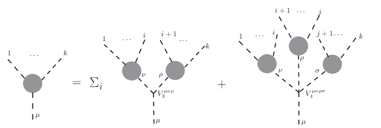
where $P_{i,j}=p_{i}+p_{i+1}+\cdots+p_{j}$ and $P_{1,k}$ is the momentum carried by the off-shell leg. A graphic description of the off-shell recursion relation is showed in Fig 1. As a recursion relation, (10) has a starting point $J^{\mu}(1)=\epsilon^{\pm\mu}(p_{1})$ , which is the current with only one on-shell gluon.

Refer to caption — Figure 1: A graphic description for the off-shell recursion relation of gluon current [Fig:division-m]

Although off-shell recursion relation is a better organization than Feynman diagrams, the calculation of $J^{\mu}\left(1,2,...,k\right)$ with general helicity configuration is still very complicated and the result is highly non-compact and gauge dependent. Nevertheless, the gauge freedom indicates that there are two helicity configurations of which results are compact under proper gauge choices. The first case is that all helicities in the current are the same, for example with positive helicities, and the result is given by

\displaystyle J^{\mu}\left(1^{+},2^{+},...,k^{+}\right)=\frac{\left\langle r|\gamma^{\mu}\not{P}_{1,k}|r\right\rangle}{\sqrt{2}\left\langle r1\right\rangle\left\langle 12\right\rangle\cdots\left\langle k-1,k\right\rangle\left\langle kr\right\rangle}\smash{\hbox to0.0pt{\raise 4.30554pt\hbox{\tiny[2.6]}\hss}}

(11)

where all reference momenta of gluons are chosen to be $r$ . The second case is that only the first gluon has negative helicity, and the current is given by

\displaystyle J^{\mu}\left(1^{-},2^{+},3^{+},...,k^{+}\right)=\frac{\langle 1|\gamma^{\mu}\not{P}_{2,k}|1\rangle}{\sqrt{2}\langle 12\rangle\cdots\langle k1\rangle}\sum_{i=3}^{k}\frac{\langle 1|\not{k}_{i}\not{P}_{1,i}|1\rangle}{P_{1,i-1}^{2}P_{1,i}^{2}}\smash{\hbox to0.0pt{\raise 4.30554pt\hbox{\tiny[2.7]}\hss}}

(12)

where reference momenta are chosen as following: $r_{1}=p_{2},\>r_{2}=r_{3}=\cdots=r_{k}=p_{1}$ . It is important to notice that for a relatively simple result, gauge choices must be made as above.

To illuminate above discussions, we give the derivation of 4-point current $J^{\mu}\left(1^{-},2^{+},3^{+},4^{+}\right)$ . To simplify the writing, we define functions $I^{\mu}[\cdot,\cdot]$ and $I^{\mu}[\cdot,\cdot,\cdot]$ as following:

	$\displaystyle I^{\mu}\left[J(1,2,...,i),J(i+1,...,k)\right]=\frac{-i}{P_{1,k}^{2}}V_{3}^{\mu\nu\rho}(P_{1,i},P_{i+1,k})J_{\nu}(1,2,...,i)J_{\rho}(i+1,...,k)$
	$\displaystyle I^{\mu}\left[J(1,2,...,i),J(i+1,...,j),J(j+1,...,k)\right]=\frac{-i}{P_{1,k}^{2}}V_{4}^{\mu\nu\rho\sigma}J_{\nu}\left(1,...,i\right)J_{\rho}\left(i+1,...,j\right)J_{\sigma}\left(j+1,...,k\right)~~\smash{\hbox to0.0pt{\raise 4.30554pt\hbox{\tiny[2.8]}\hss}}$		(13)

Thus the off-shell recursion relation given in (10) could be written as

\displaystyle J^{\mu}\left(1,2,...,k\right)=\sum_{i}I^{\mu}[J(1,2,...,i),J(i+1,...,k)]+\sum_{i,j}I^{\mu}[J(1,2,...,i),J(i+1,...,j),J(j+1,...,k)]~~\smash{\hbox to0.0pt{\raise 4.30554pt\hbox{\tiny[2.9]}\hss}}

(14)

With this notation, the 4-point current $J^{\mu}(1,2,3,4)$ could be written recursively as

	$\displaystyle J^{\mu}\left(1,2,3,4\right)$	$\displaystyle=$	$\displaystyle I^{\mu}\left[J(1),J\left(2,3,4\right)\right]+I^{\mu}\left[J\left(1,2\right),J\left(3,4\right)\right]+I^{\mu}\left[J\left(1,2,3\right),J(4)\right]$		(15)
			$\displaystyle+I^{\mu}\left[J(1),J(2),J\left(3,4\right)\right]+I^{\mu}\left[J(1),J\left(2,3\right),J(4)\right]+I^{\mu}\left[J\left(1,2\right),J(3),J(4)\right]$		(15)

For the helicity configuration $\left(1^{-},2^{+},3^{+},4^{+}\right)$ we choose the reference momenta as $r_{1}=p_{2},\>r_{2}=r_{3}=r_{4}=p_{1}$ , then it is not difficult to check that following four terms vanish

	$\displaystyle I^{\mu}\left[J\left(1^{-},2^{+}\right),J\left(3^{+},4^{+}\right)\right]=I^{\mu}\left[J(1^{-}),J(2^{+}),J\left(3^{+},4^{+}\right)\right]$
	$\displaystyle=I^{\mu}\left[J(1^{-}),J\left(2^{+},3^{+}\right),J(4^{+})\right]=I^{\mu}\left[J\left(1^{-},2^{+}\right),J(3^{+}),J(4^{+})\right]=0$		(16)

while the other two non vanishing terms are given as

	$\displaystyle I^{\mu}\left[J(1^{-}),J\left(2^{+},3^{+},4^{+}\right)\right]$	$\displaystyle=$	$\displaystyle-\frac{\langle 1\|3+4\|2]\langle 1\|\gamma^{\mu}\not{k}_{234}\|1\rangle}{\sqrt{2}s_{1234}s_{12}\langle 23\rangle\langle 34\rangle\langle 41\rangle}$		(17)
	$\displaystyle I^{\mu}\left[J\left(1^{-},2^{+},3^{+}\right),J(4^{+})\right]$	$\displaystyle=$	$\displaystyle\frac{[23]\langle 1\|2+3\|4]}{\sqrt{2}s_{12}s_{123}s_{1234}\langle 14\rangle\langle 23\rangle}\langle 1\|\gamma^{\mu}\not{k}_{234}\|1\rangle$		(18)

Adding them up we obtain

	$\displaystyle J^{\mu}\left(1^{-},2^{+},3^{+},4^{+}\right)$	$\displaystyle=$	$\displaystyle I^{\mu}\left[1^{-},\left(2^{+},3^{+},4^{+}\right)\right]+I^{\mu}\left[\left(1^{-},2^{+},3^{+}\right),4^{+}\right]$		(19)
		$\displaystyle=$	$\displaystyle\frac{\langle 1\|\gamma^{\mu}\not{k}_{234}\|1\rangle}{\sqrt{2}\langle 12\rangle\langle 23\rangle\langle 34\rangle\langle 41\rangle}\left(\frac{\langle 1\|\not{3}\cdot\left(\not{1}+\not{2}+\not{3}\right)\|1\rangle}{s_{12}s_{123}}+\frac{\langle 1\|\not{4}\cdot\left(\not{1}+\not{2}+\not{3}+\not{4}\right)\|1\rangle}{s_{123}s_{1234}}\right)$		(19)

which is the one given by (12).

Having shown the calculation of current by off-shell recursion relation, it is natural to ask if we can do it using the new discovered on-shell recursion technique. In following two subsections, we will discuss this issue.

2.1 Recursion relation by two on-shell gluon deformation

[Onshell]

The off-shell current $J^{\mu}(1,2,...,k)$ has $k$ on-shell gluons, thus it is obvious that we can take a pair of on-shell gluons to do the BCFW-deformation and write down the corresponding BCFW recursion relation for the current. The boundary behavior under the deformation $\left[i|j\right\rangle$ (i.e., the deformation $\left|i\right]\to\left|i\right]-z\left|j\right]$ , $\left|j\right\rangle\to\left|j\right\rangle+z\left|i\right\rangle$ ) will be ${1\over z}$ for the helicity configurations $(-,+),(+,+),(-,-)$ and $z^{3}$ for the helicity configuration $(+,-)$ ⁵⁵ 5 The boundary behavior is, in fact, more subtle. For example, if $(i,j)$ are not nearby, we will have ${1\over z^{2}}$ behavior for $(-,+),(+,+),(-,-)$ . But for our purpose, naive counting is enough. and the off-shell leg will not cause any trouble.

With above explanation, if the helicity of $(1,k)$ is $\left(-,+\right)$ , $\left(-,-\right)$ and $\left(+,+\right)$ , we can take the deformation on $1$ and $k$

\displaystyle|1]

\displaystyle\rightarrow

\displaystyle|1]-z|k],\;|k\rangle\rightarrow|k\rangle+z|1\rangle

(20)

and the corresponding recursion relation is given by

	$\displaystyle J^{\mu}\left(1,2,...,k\right)$	$\displaystyle=$	$\displaystyle\sum_{i=2}^{k-1}\sum_{h,\widetilde{h}}\left[A\left(\widehat{1},...,i,\widehat{P}^{h}\right)\cdot\frac{1}{P_{1,i}^{2}}\cdot J^{\mu}\left(-\widehat{P}^{\widetilde{h}},i+1,...,\widehat{k}\right)\right.$
	$\displaystyle+J^{\mu}\left(\widehat{1},...,i,\widehat{P}^{h}\right)$		$\displaystyle\left.\cdot\frac{1}{P_{i+1,k}^{2}}\cdot A\left(-\widehat{P}^{\widetilde{h}},i+1,...,\widehat{k}\right)\right],~~(h,\widetilde{h})=(+,-),(-,+),(L,T),(T,L)~~\smash{\hbox to0.0pt{\raise 4.30554pt\hbox{\tiny[2.16]}\hss}}$		(21)

where the graphic description is given in Fig 2.

There are several things we need to emphasize for the formula (21). First, since the current $J^{\mu}\left(1,2,...,k\right)$ itself is gauge dependent, all reference momenta in the sub-currents at the right hand side of (21) must be the same with these at the left hand side of (21). A consequence of this requirement is that we can not naively use results (11) and (12), which are results with special choices of gauge.

Secondly, for the on-shell momentum $\widehat{P}$ at the right hand side of (21), we must sum over four polarization vectors defined in (3) and (5) (not just the vectors in (3)) by the formula (8) for Feynman propagator. The reason that we can neglect the sum over vectors in (5) for on-shell amplitude is because $\epsilon^{L}=\widehat{P}$ and by the Ward Identity, when all other particles are on-shell and with physical polarizations, $\widehat{P}\cdot A=0$ . Thus for other two configurations $(h,\widetilde{h})=(L,T),(T,L)$ in (21), we have either the $\widehat{P}\cdot A_{L}=0$ or $\widehat{P}\cdot A_{R}=0$ , so we are left with only two familiar helicity configurations in BCFW recursion relation for on-shell amplitudes. For off-shell current we are interesting in, we do not have $\epsilon^{L,T}\cdot J\neq 0$ , thus we can not neglect the sum over $(h,\widetilde{h})=(L,T),(T,L)$ . However, we will show that usually these two terms can vanish by special choice of gauge. Also in the practice we should use the Ward Identity to simplify the calculation. For example, with $(h,\tilde{h})=(T,L)$ configuration the second term of (21) vanishes according to Ward Identity

\displaystyle A\left(-\widehat{P}^{L},i+1,...,\widehat{k}\right)=-\widehat{P}^{L}_{\mu}\cdot M^{\mu}\left(i+1,...,\widehat{k}\right)=0

(22)

Because we have summed over all four polarization vectors, the result (21) does not depend on the gauge choice of $P$ and we can choose gauge freely. The building block of (21) is three-point on-shell amplitude and $J^{\mu}(1,2)$ . Without a loss of generality, two-point off-shell currents are given as

$\displaystyle J^{\mu}\left(1^{-},2^{+}\right)$	$\displaystyle=$	$\displaystyle\frac{1}{\sqrt{2}s_{12}}\left(\frac{[r_{1}2]\langle 1r_{2}\rangle}{[r_{1}1]\langle r_{2}2\rangle}\left(1-2\right)^{\mu}+\frac{[2r_{1}]\langle 21\rangle}{[r_{1}1]\langle r_{2}2\rangle}\langle r_{2}\|\gamma^{\mu}\|2]+\frac{[12]\langle r_{2}1\rangle}{[r_{1}1]\langle r_{2}2\rangle}[r_{1}\|\gamma^{\mu}\|1\rangle\right)\smash{\hbox to0.0pt{\raise 4.30554pt\hbox{\tiny[3.17]}\hss}}$	(23)
$\displaystyle J^{\mu}\left(1^{+},2^{+}\right)$	$\displaystyle=$	$\displaystyle\frac{1}{\sqrt{2}s_{12}}\left(\frac{[12]\langle r_{2}r_{1}\rangle}{\langle r_{1}1\rangle\langle r_{2}2\rangle}\left(1-2\right)^{\mu}+\frac{[21]\langle r_{1}2\rangle}{\langle r_{1}1\rangle\langle r_{2}2\rangle}\langle r_{2}\|\gamma^{\mu}\|2]+\frac{[21]\langle r_{2}1\rangle}{\langle r_{1}1\rangle\langle r_{2}2\rangle}\langle r_{1}\|\gamma^{\mu}\|1]\right)~~\smash{\hbox to0.0pt{\raise 4.30554pt\hbox{\tiny[2.18]}\hss}}$	(24)
$\displaystyle J^{\mu}\left(1^{-},2^{T}\right)$	$\displaystyle=$	$\displaystyle\frac{1}{\sqrt{2}s_{12}}\left(-\frac{\left\langle 12\right\rangle\left[2r_{1}\right]}{\left[r_{1}1\right]}\left(1+2\right)^{\mu}+\frac{\left\langle 12\right\rangle\left[21\right]}{\left[r_{1}1\right]}\left\langle 1\|\gamma^{\mu}\|r_{1}\right]\right)~~\smash{\hbox to0.0pt{\raise 4.30554pt\hbox{\tiny[2.18-1]}\hss}}$	(25)
$\displaystyle J^{\mu}\left(1^{+},2^{T}\right)$	$\displaystyle=$	$\displaystyle\frac{1}{\sqrt{2}s_{12}}\left(\frac{\left\langle r_{1}2\right\rangle\left[21\right]}{\left\langle r_{1}1\right\rangle}\cdot\left(1+2\right)^{\mu}-\frac{\left\langle 12\right\rangle\left[21\right]}{\left\langle r_{1}1\right\rangle}\left\langle r_{1}\|\gamma^{\mu}\|1\right]\right)~~\smash{\hbox to0.0pt{\raise 4.30554pt\hbox{\tiny[2.18-2]}\hss}}$	(26)

where the gauge of each on-shell gluon has kept. Having established the general idea for recursion relation, we present two examples.

Example 1

The first example is three-point current $J^{\mu}\left(1^{+},2^{+},3^{+}\right)$ . With the deformation on $p_{1}$ and $p_{2}$ ,

\displaystyle|1]\rightarrow|1]-z|2],\,|2\rangle\rightarrow|2\rangle+z|1\rangle

(27)

we can write down the recursion relation as

	$\displaystyle J^{\mu}\left(1^{+},2^{+},3^{+}\right)=J^{\mu}\left(\widehat{1}^{+},\widehat{P}^{+}\right)\cdot\frac{1}{s_{23}}\cdot A\left(-\widehat{P}^{-},\widehat{2}^{+},3^{+}\right)$
	$\displaystyle+J^{\mu}\left(\widehat{1}^{+},\widehat{P}^{-}\right)\cdot\frac{1}{s_{23}}\cdot A\left(-\widehat{P}^{+},\widehat{2}^{+},3^{+}\right)$
	$\displaystyle+J^{\mu}\left(\widehat{1}^{+},\widehat{P}^{L}\right)\cdot\frac{1}{s_{23}}\cdot A\left(-\widehat{P}^{T},\widehat{2}^{+},3^{+}\right)$
	$\displaystyle+J^{\mu}\left(\widehat{1}^{+},\widehat{P}^{T}\right)\cdot\frac{1}{s_{23}}\cdot A\left(-\widehat{P}^{L},\widehat{2}^{+},3^{+}\right)~~~\smash{\hbox to0.0pt{\raise 4.30554pt\hbox{\tiny[J-Exa1-1]}\hss}}$		(28)

here $\widehat{P}^{L}$ and $\widehat{P}^{T}$ are longitude and timelike vectors of the new gluon $\widehat{P}$ . We note here that as the external gluons are color-ordered, the order in the current is constrained which leads to only one pole appear in the recursion relation above, i.e., there is no term $A(3^{+},\widehat{1}^{+},\widehat{P}^{h}){1\over s_{13}}J^{\mu}(-\widehat{P}^{\widetilde{h}},2)$ .

For the four terms in (28), the second term is zero with all positive helicities and the fourth term is zero by Ward Identity. Then the recursion relation is given only by

\displaystyle J^{\mu}\left(1^{+},2^{+},3^{+}\right)=J^{\mu}\left(\widehat{1}^{+},\widehat{P}^{+}\right)\cdot\frac{1}{s_{23}}\cdot A\left(-\widehat{P}^{-},\widehat{2}^{+},3^{+}\right)+J^{\mu}\left(\widehat{1}^{+},\widehat{P}^{L}\right)\cdot\frac{1}{s_{23}}\cdot A\left(-\widehat{P}^{T},\widehat{2}^{+},3^{+}\right)

(29)

To check the $\widehat{P}$ -gauge independent of result we set the reference momentum of the new gluon $\widehat{P}$ to be an arbitrary null vector $q$ and reference momenta of external particles to be $r_{1}=r_{2}=r_{3}=r$ , thus two terms are respectively given by

	$\displaystyle J^{\mu}\left(\widehat{1}^{+},\widehat{P}^{+}\right)\cdot\frac{1}{s_{23}}\cdot A\left(-\widehat{P}^{-},\widehat{2}^{+},3^{+}\right)$
	$\displaystyle=\frac{1}{\sqrt{2}s_{\widehat{1}\widehat{P}}}\left(\frac{\left[\widehat{P}\widehat{1}\right]\left\langle rq\right\rangle}{\left\langle r\widehat{1}\right\rangle\left\langle q\widehat{P}\right\rangle}\left(\widehat{1}-\widehat{P}\right)^{\mu}+\frac{\left[\widehat{1}\widehat{P}\right]\left\langle\widehat{P}r\right\rangle}{\left\langle r\widehat{1}\right\rangle\left\langle q\widehat{P}\right\rangle}\left\langle q\|\gamma^{\mu}\|\widehat{P}\right]+\frac{\left[\widehat{1}\widehat{P}\right]\left\langle\widehat{1}q\right\rangle}{\left\langle r\widehat{1}\right\rangle\left\langle q\widehat{P}\right\rangle}\left\langle r\|\gamma^{\mu}\|\widehat{1}\right]\right)\cdot\frac{1}{s_{23}}\cdot\frac{\left[\widehat{2}3\right]^{3}}{\left[\widehat{2}\widehat{P}\right]\left[\widehat{P}3\right]}\;,\;$		(30)
	$\displaystyle J^{\mu}\left(\widehat{1}^{+},\widehat{P}^{L}\right)\cdot\frac{1}{s_{23}}\cdot A\left(-\widehat{P}^{T},\widehat{2}^{+},3^{+}\right)$
	$\displaystyle=-\frac{1}{\sqrt{2}s_{\widehat{1}\widehat{P}}}\left(\frac{\left\langle r\widehat{P}\right\rangle[\widehat{P}\widehat{1}]}{\left\langle r\widehat{1}\right\rangle}\cdot\left(\widehat{1}+\widehat{P}^{L}\right)^{\mu}-\frac{\left\langle\widehat{1}\widehat{P}\right\rangle[\widehat{P}\widehat{1}]}{\left\langle r\widehat{1}\right\rangle}\left\langle r\|\gamma^{\mu}\|\widehat{1}\right]\right)\cdot\frac{1}{s_{23}}\cdot\frac{\left\langle qr\right\rangle\left[\widehat{2}3\right]\left\langle r\widehat{P}\right\rangle}{\left\langle q\widehat{P}\right\rangle\left\langle r3\right\rangle\left\langle r\widehat{2}\right\rangle}~~~\smash{\hbox to0.0pt{\raise 4.30554pt\hbox{\tiny[gauge-extra-1]}\hss}}$		(31)

There are several things we want to discuss regarding this result. First the $q$ -gauge independent can be numerically checked using the package S@M [21] and indeed it is given by

	$\displaystyle J^{\mu}\left(1^{+},2^{+},3^{+}\right)$	$\displaystyle=$	$\displaystyle J^{\mu}\left(\widehat{1}^{+},\widehat{P}^{+}\right)\cdot\frac{1}{s_{23}}\cdot A\left(-\widehat{P}^{-},\widehat{2}^{+},3^{+}\right)+J^{\mu}\left(\widehat{1}^{+},\widehat{P}^{L}\right)\cdot\frac{1}{s_{23}}\cdot A\left(-\widehat{P}^{T},\widehat{2}^{+},3^{+}\right)$		(32)
		$\displaystyle=$	$\displaystyle\frac{\langle r\|\gamma^{\mu}\not{k}_{123}\|r\rangle}{\sqrt{2}\langle r1\rangle\langle 12\rangle\langle 23\rangle\langle 3r\rangle}$		(32)

as we expected. We have seen that to achieve the $q$ -gauge independent, the second term is very crucial with the unfamiliar $A\left(-\widehat{P}^{T},\widehat{2}^{+},3^{+}\right)$ . In particular, the gauge choice of gluon $2,3$ will effect the whole result through $A\left(-\widehat{P}^{T},\widehat{2}^{+},3^{+}\right)$ , which is not gauge invariant.

Secondly, it’s very obvious that with $q=r$ , the second term (31) vanishes, thus the result is given just by familiar on-shell BCFW recursion relation for amplitude

$\displaystyle J^{\mu}\left(1^{+},2^{+},3^{+}\right)$	$\displaystyle=$	$\displaystyle J^{\mu}\left(\widehat{1}^{+},\widehat{P}^{+}\right)\cdot\frac{1}{s_{23}}\cdot A\left(-\widehat{P}^{-},\widehat{2}^{+},3^{+}\right)$	(33)
	$\displaystyle=$	$\displaystyle\frac{1}{\sqrt{2}\langle 1\widehat{P}\rangle}\left(\frac{\langle r\|\gamma^{\mu}\|\widehat{P}]}{\langle r1\rangle}+\frac{\langle r\|\gamma^{\mu}\|\widehat{1}]}{\langle r\widehat{P}\rangle}\right)\cdot\frac{1}{s_{23}}\cdot-\frac{[\widehat{2}3]}{[3\widehat{P}][\widehat{P}\widehat{2}]}$
	$\displaystyle=$	$\displaystyle\frac{\langle r\|\gamma^{\mu}\not{k}_{123}\|r\rangle}{\sqrt{2}\langle r1\rangle\langle 12\rangle\langle 23\rangle\langle 3r\rangle}$

We must emphasize this is true when and only when we choose the special gauge.

Example 2

Using the same method to the current $J^{\mu}\left(1^{-},2^{+},3^{+}\right)$ , with the same deformation

|1]\rightarrow|1]-z|2],\,|2\rangle\rightarrow|2\rangle+z|1\rangle

the recursion relation is given as

	$\displaystyle J^{\mu}\left(1^{-},2^{+},3^{+}\right)=J^{\mu}\left(\widehat{1}^{-},\widehat{P}^{+}\right)\cdot\frac{1}{s_{23}}\cdot A\left(-\widehat{P}^{-},\widehat{2}^{+},3^{+}\right)$
	$\displaystyle+J^{\mu}\left(\widehat{1}^{-},\widehat{P}^{-}\right)\cdot\frac{1}{s_{23}}\cdot A\left(-\widehat{P}^{+},\widehat{2}^{+},3^{+}\right)$
	$\displaystyle+J^{\mu}\left(\widehat{1}^{-},\widehat{P}^{L}\right)\cdot\frac{1}{s_{23}}\cdot A\left(-\widehat{P}^{T},\widehat{2}^{+},3^{+}\right)$
	$\displaystyle+J^{\mu}\left(\widehat{1}^{-},\widehat{P}^{T}\right)\cdot\frac{1}{s_{23}}\cdot A\left(-\widehat{P}^{L},\widehat{2}^{+},3^{+}\right)\smash{\hbox to0.0pt{\raise 4.30554pt\hbox{\tiny[3.23]}\hss}}$		(34)

where again color-ordering leads to only one cut $s_{23}$ as above. In (34) the second vanishes with all positive helicity while the fourth term vanishes by Ward Identity. With general reference null momentum of the new gluon $\widehat{P}$ , the first and third terms are given as

	$\displaystyle J^{\mu}\left(\widehat{1}^{-},\widehat{P}^{+}\right)\cdot\frac{1}{s_{23}}\cdot A\left(-\widehat{P}^{-},\widehat{2}^{+},3^{+}\right)$
	$\displaystyle=\frac{1}{\sqrt{2}s_{\widehat{1}\widehat{P}}}\left[-\frac{\left\langle\widehat{1}q\right\rangle\left[\widehat{P}\widehat{2}\right]}{\left[\widehat{2}\widehat{1}\right]\left\langle q\widehat{P}\right\rangle}\left(\widehat{1}-\widehat{P}\right)^{\mu}-\frac{\left\langle\widehat{P}\widehat{1}\right\rangle\left[\widehat{2}\widehat{P}\right]}{\left\langle q\widehat{P}\right\rangle\left[\widehat{2}\widehat{1}\right]}\left\langle q\|\gamma^{\mu}\|\widehat{P}\right]+\frac{\left\langle\widehat{1}q\right\rangle\left[\widehat{P}\widehat{1}\right]}{\left[\widehat{2}\widehat{1}\right]\left\langle q\widehat{P}\right\rangle}\left\langle\widehat{1}\|\gamma^{\mu}\|\widehat{2}\right]\right]\cdot\frac{1}{s_{23}}\cdot\frac{\left[\widehat{2}3\right]^{3}}{\left[\widehat{2}\widehat{P}\right]\left[\widehat{P}3\right]}$
	$\displaystyle J^{\mu}\left(\widehat{1}^{-},\widehat{P}^{L}\right)\cdot\frac{1}{s_{23}}\cdot A\left(-\widehat{P}^{T},\widehat{2}^{+},3^{+}\right)$
	$\displaystyle=\frac{1}{\sqrt{2}s_{\widehat{1}\widehat{P}}}\left[-\frac{\left\langle\widehat{1}\widehat{P}\right\rangle\left[\widehat{P}\widehat{2}\right]}{\left[\widehat{2}\widehat{1}\right]}\left(\widehat{1}+\widehat{P}\right)^{\mu}+\frac{\left\langle\widehat{1}\widehat{P}\right\rangle\left[\widehat{P}\widehat{1}\right]}{\left[\widehat{2}\widehat{1}\right]}\left\langle\widehat{1}\|\gamma^{\mu}\|\widehat{2}\right]\right]\cdot\frac{1}{s_{23}}\cdot\frac{\left\langle\widehat{P}\widehat{1}\right\rangle\left\langle q\widehat{1}\right\rangle\left[\widehat{2}3\right]}{\left\langle\widehat{P}q\right\rangle\left\langle\widehat{1}\widehat{2}\right\rangle\left\langle\widehat{1}3\right\rangle}~~~\smash{\hbox to0.0pt{\raise 4.30554pt\hbox{\tiny[1.33-1.33]}\hss}}$		(35)

and it is numerically checked that the result is $q$ -gauge invariant. Recall that by (23), a good gauge choosing of current $J^{\mu}\left(1^{-},2^{+},3^{+}\right)$ is $r_{1}=p_{2}$ , $r_{2}=r_{3}=p_{1}$ . Also by checking (35) it is easy to see that when we choose $q=p_{1}$ , many terms will be zero. Putting this choice back we get immediately

\displaystyle J^{\mu}\left(1^{-},2^{+},3^{+}\right)=\frac{\left[32\right]\left\langle 1|\gamma^{\mu}\not{k}_{123}|1\right\rangle}{\sqrt{2}s_{12}s_{123}\left\langle 23\right\rangle}

(36)

Again, we find the results from on-shell recursion relation and off-shell recursion relation match with each other.

From above two examples, it is easy to see that although with off-shell current, which is not gauge invariant, we need to sum over four helicity configurations in recursion relation, there is gauge freedom of $\widehat{P}$ we can choose to eliminate many middle contributions. Properly using of this observation will simplify calculations.

2.2 On shell recursion relation involving the off shell leg

Through derivation above, we show that BCFW recursion relation is valid for the gluon current with deformation of two on-shell particles. However as a gluon current contains an off shell leg, there seems to be another deformation we can make such that $z$ -dependent momentum flux goes through the current from an on-shell particle to the off shell leg. In this part we will exhibit how this could be realized and what’s the recursion relation it will imply.

To find the recursion relation involving the off shell leg in a current, we consider an one-particle shifting deformation. Without loss of generality, we assume the first gluon in the current has $+$ helicity. For such a current $J^{\mu}(1^{+},2,...,k)$ , we do the deformation as

\displaystyle|1\rangle\rightarrow|1\rangle+z|q\rangle

(37)

where $|q\rangle$ is the left-handed spinor of a arbitrary lightlike momentum $q$ . At this momentum, it seems that $q$ can be chosen arbitrarily, but from explicit results, for example (11), we can see that there is unphysical pole, for example $\left\langle r|1\right\rangle$ , shown up. To get rid of this phenomenon and keep only physical pole, we should choose $q$ to be the same gauge choice for the definition of positive helicity of particle $1$ .

This deformation has kept the on-shell condition for particle $1$ , and there is no requirement of momentum conservation because the off-shell momentum is allowed to change. With this deformation, the polarization vector will behave as

\displaystyle\epsilon_{1}^{+\mu}=\frac{\langle r_{1}|\gamma^{\mu}|p_{1}]}{\sqrt{2}\langle r_{1}p_{1}\rangle}\sim\frac{1}{z}

(38)

for large $z$ . To consider the large $z$ -behavior, we consider the path from $1$ to off-shell leg with only most dangerous cubic vertexes, since each propagator contributes $\frac{1}{z}$ and each cubic vertex contributes $z$ , the overall $z$ behavior will be $\frac{1}{z}\cdot z^{i}\cdot\frac{1}{z^{i}}=\frac{1}{z}$ . ⁶⁶ 6 For the case that the first gluon has $-$ helicity, the deformation should be $|1]\rightarrow|1]-z|q]$ so the polarization will behave as $\epsilon_{1}^{-\mu}=-\frac{[r_{1}|\gamma^{\mu}|p_{1}\rangle}{\sqrt{2}[r_{1}p_{1}]}\sim\frac{1}{z}$ .

With the good behavior, the recursion relation is given as

\displaystyle J^{\mu}(1,2,...,k)=\sum_{i}\sum_{h,\tilde{h}}A(\widehat{1},2,...,i-1,\widehat{P}^{h})\cdot\frac{1}{P_{1,i-1}^{2}}\cdot J^{\mu}(-\widehat{P}^{\tilde{h}},i,...,k),~~~~\smash{\hbox to0.0pt{\raise 4.30554pt\hbox{\tiny[3.28]}\hss}}

(39)

where the sum is over $(h,\widetilde{h})=(+,-),(-,+),(L,T),(T,L)$ for exact same reason as in previous subsection. Different from the recursion relation in (21), there is only one term and only three shifted momenta $\widehat{1},\widehat{P}^{h},-\widehat{P}^{-\tilde{h}}$ instead of four. Also the off-shell momentum will be $z$ -dependent, thus we will have following $z$ -dependent propagator

\displaystyle D^{\mu\nu}(p-zl)=\frac{-ig^{\mu\nu}}{P^{2}-2zl\cdot p},~~~l=\left|q\right\rangle\left|1\right]

(40)

in Feynman gauge, which will contribute to the residue. Finally because the color ordering, the deformation with $1$ will give minimum number of terms, but we could choose arbitrary on-shell particle, which will be discussed in an example.

Having established (39) we give some examples.

Example 1 $J^{\mu}(1,2)\rightarrow J^{\mu}(1)$

Let us start with the two-point current $J^{\mu}(1,2)$ which is the simplest example. As for $J^{\mu}(1^{+},2^{+})$ , a usual gauge choosing is $r_{1}=r_{2}=r$ , so we take the deformation as

\displaystyle|1\rangle\rightarrow|1\rangle+z|r\rangle

(41)

to avoid unwanted unphysical pole. The recursion relation is given by

\displaystyle J^{\mu}(1^{+},2^{+})=A(\widehat{1}^{+},2^{+},\widehat{P}^{-})\cdot\frac{1}{s_{12}}\cdot J^{\mu}(-\widehat{P}^{+})+A(\widehat{1}^{+},2^{+},\widehat{P}^{T})\cdot\frac{1}{s_{12}}\cdot J^{\mu}(-\widehat{P}^{L})

(42)

where another two helicity configurations are zero. Without gauge choosing of $P$ , the result is

\displaystyle J^{\mu}\left(1^{+},2^{+}\right)=\frac{\left[\widehat{1}2\right]^{3}}{\left[\widehat{1}\widehat{P}\right]\left[\widehat{P}2\right]}\cdot\frac{1}{s_{12}}\cdot\frac{\left\langle q|\gamma^{\mu}|\widehat{P}\right]}{\sqrt{2}\left\langle q\widehat{P}\right\rangle}+\frac{\sqrt{2}\left\langle qr\right\rangle\left[\widehat{1}2\right]\left\langle r\widehat{P}\right\rangle}{\left\langle q\widehat{P}\right\rangle\left\langle r\widehat{1}\right\rangle\left\langle r2\right\rangle}\cdot\frac{1}{s_{12}}\cdot\frac{\left\langle\widehat{P}|\gamma^{\mu}|\widehat{P}\right]}{2}

(43)

which can be checked to be $q$ -gauge independent by Mathematica. To simplify analytically, we can choose the convenient gauge $q_{\widehat{P}}=r$ , so the second term vanishes and the result is

\displaystyle J^{\mu}(1^{+},2^{+})

\displaystyle=

\displaystyle-\frac{\left[12\right]^{3}}{\left[2\widehat{P}\right]\left[\widehat{P}1\right]}\cdot\frac{1}{s_{12}}\cdot\frac{\left\langle r|\gamma^{\mu}|\widehat{P}\right]}{\sqrt{2}\left\langle r\widehat{P}\right\rangle}=\frac{\left\langle r|\gamma^{\mu}\not{P}_{12}|r\right\rangle}{\sqrt{2}\left\langle r1\right\rangle\left\langle 12\right\rangle\left\langle 2r\right\rangle}

(44)

There is one technical issue with the choice $q=r$ . Naively the deformed polarization vector behaves as $\epsilon_{1}^{\mu}\sim z^{0}$ which seems to destroy the good large $z$ behavior. However the first cubic vertex connecting $1$ and $2$ now is also behaves as $z^{0}$ instead of $z^{1}$

	$\displaystyle V_{3}(z)$	$\displaystyle=$	$\displaystyle\frac{i}{\sqrt{2}}\left[\eta^{\nu\rho}\cdot(p_{1}-p_{2})^{\mu}+2\eta^{\rho\mu}\cdot p_{2}^{\nu}-2\eta^{\mu\nu}\cdot p_{1}^{\rho}\right]\cdot\epsilon_{1\nu}\cdot\epsilon_{2\rho}$		(45)
		$\displaystyle=$	$\displaystyle\sqrt{2}i\epsilon_{2}^{\mu}\cdot(p_{2}\cdot\epsilon_{1})\sim\ z^{0}~,$		(45)

thus the whole $z$ behavior is still $\frac{1}{z}$ and the recursion relation is still valid.

Example 2 $J^{\mu}(1,2,3)\rightarrow J^{\mu}(1,2)$

For this example, we will consider different choices of deformations.

a. $J^{\mu}(1^{+},2^{+},3^{+})$ with with deformation on $1^{+}$

With deformation (41) there are two poles in the current so the recursion relation is given as

	$\displaystyle J^{\mu}(1^{+},2^{+},3^{+})=A(\widehat{1}^{+},2^{+},\widehat{P}^{-})\cdot\frac{1}{s_{12}}\cdot J^{\mu}(-\widehat{P}^{+},3^{+})$
	$\displaystyle+A(\widehat{1}^{+},2^{+},\widehat{P}^{T})\cdot\frac{1}{s_{12}}\cdot J^{\mu}(-\widehat{P}^{L},3^{+})$
	$\displaystyle+A(\widehat{1}^{+},2^{+},3^{+},\widehat{P}^{T})\cdot\frac{1}{s_{123}}\cdot J^{\mu}(-\widehat{P}^{L})$		(46)

where among eight possible contributions we have kept only three with nonzero contributions. With general reference momentum $q$ of the new gluon $\widehat{P}$ , these three terms are given by

	$\displaystyle A(\widehat{1}^{+},2^{+},\widehat{P}^{-})\cdot\frac{1}{s_{12}}\cdot J^{\mu}(-\widehat{P}^{+},3^{+})$
	$\displaystyle=-\frac{\left[\widehat{1}2\right]^{3}}{\left[2\widehat{P}\right]\left[\widehat{P}\widehat{1}\right]}\cdot\frac{1}{s_{12}}\cdot\frac{1}{\sqrt{2}s_{3\widehat{P}}}\left(\frac{\left[\widehat{P}3\right]\left\langle rq\right\rangle}{\left\langle q\widehat{P}\right\rangle\left\langle r3\right\rangle}\left(\widehat{P}-3\right)^{\mu}+\frac{\left[3\widehat{P}\right]\left\langle q3\right\rangle}{\left\langle q\widehat{P}\right\rangle\left\langle r3\right\rangle}\left\langle r\|\gamma^{\mu}\|3\right]+\frac{\left[3\widehat{P}\right]\left\langle r\widehat{P}\right\rangle}{\left\langle q\widehat{P}\right\rangle\left\langle r3\right\rangle}\left\langle q\|\gamma^{\mu}\|\widehat{P}\right\rangle\right)$		(47)
	$\displaystyle A(\widehat{1}^{+},2^{+},\widehat{P}^{T})\cdot\frac{1}{s_{12}}\cdot J^{\mu}(-\widehat{P}^{L},3^{+})$
	$\displaystyle=\frac{\left[\widehat{1}2\right]\left\langle qr\right\rangle\left\langle\widehat{P}r\right\rangle}{\left\langle r\widehat{1}\right\rangle\left\langle 2r\right\rangle\left\langle\widehat{P}q\right\rangle}\cdot\frac{1}{s_{12}}\cdot\frac{1}{\sqrt{2}s_{3\widehat{P}}}\left(\frac{\left\langle r\widehat{P}\right\rangle\left[\widehat{P}3\right]}{\left\langle r3\right\rangle}\left(3+\widehat{P}\right)^{\mu}-\frac{\left\langle 3\widehat{P}\right\rangle\left[\widehat{P}3\right]}{r3}\left\langle r\|\gamma^{\mu}\|3\right]\right)$		(48)
	$\displaystyle A(\widehat{1}^{+},2^{+},3^{+},\widehat{P}^{T})\cdot\frac{1}{s_{123}}\cdot J^{\mu}(-\widehat{P}^{L})$
	$\displaystyle=\frac{1}{\sqrt{2}}\cdot\frac{\left\langle rq\right\rangle\left\langle\widehat{P}r\right\rangle}{\left\langle r\widehat{1}\right\rangle\left\langle\widehat{1}2\right\rangle\left\langle 23\right\rangle\left\langle 3r\right\rangle}\cdot\left\langle\widehat{P}\|\gamma^{\mu}\|\widehat{P}\right]$		(49)

and we have checked that the sum is same for any choice of $q$ . We can simplify result by choosing the gauge of $P$ to be $r_{\widehat{P}}=r_{1}=r_{2}=r_{3}=r$ and again, the second and third terms vanish with factor $\left\langle qr\right\rangle$ . Finally we have

	$\displaystyle J^{\mu}(1^{+},2^{+},3^{+})$	$\displaystyle=$	$\displaystyle-\frac{\left[12\right]^{3}}{\left[2\widehat{P}\right]\left[\widehat{P}1\right]}\cdot\frac{1}{s_{12}}\cdot\frac{1}{\sqrt{2}s_{3\widehat{P}}}\left(\frac{\left[3\widehat{P}\right]}{\left\langle r\widehat{P}\right\rangle}\left\langle r\|\gamma^{\mu}\|3\right]+\frac{[3\widehat{P}]}{\left\langle r3\right\rangle}\left\langle r\|\gamma^{\mu}\|\widehat{P}\right]\right)$		(50)
		$\displaystyle=$	$\displaystyle\frac{\left\langle r\|\gamma^{\mu}\not{P}_{123}\|r\right\rangle}{\sqrt{2}\left\langle r1\right\rangle\left\langle 12\right\rangle\left\langle 23\right\rangle\left\langle 3r\right\rangle}$		(50)

which gives the right result.

b. $J^{\mu}(1^{+},2^{+},3^{+})$ with deformation on $2^{+}$

If we consider the same current $J^{\mu}(1^{+},2^{+},3^{+})$ with deformation

\displaystyle|2\rangle\rightarrow|2\rangle+z|r\rangle

(51)

the recursion relation then will contain different poles. Among many terms, there with nonzero contributions are

$\displaystyle J^{\mu}(1^{+},2^{+},3^{+})=$	$\displaystyle A(1^{+},\widehat{2}^{+},\widehat{P}^{-})\cdot\frac{1}{s_{12}}\cdot J^{\mu}(-\widehat{P}^{+},3^{+})+A(1^{+},\widehat{2}^{+},\widehat{P}^{T})\cdot\frac{1}{s_{12}}\cdot J^{\mu}(-\widehat{P}^{L},3^{+})$	(52)
	$\displaystyle+J^{\mu}(1^{+},-\widehat{P}^{+})\cdot\frac{1}{s_{23}}\cdot A(\widehat{P}^{-},\widehat{2}^{+},3^{+})+J^{\mu}(1^{+},-\widehat{P}^{L})\cdot\frac{1}{s_{23}}\cdot A(\widehat{P}^{T},\widehat{2}^{+},3^{+})$
	$\displaystyle+A(1^{+},\widehat{2}^{+},3^{+},\widehat{P}^{T})\cdot\frac{1}{s_{123}}\cdot J^{\mu}(-\widehat{P}^{L})$

with following explicit expressions⁷⁷ 7 In principle, the reference momenta for $\widehat{P}_{12},\widehat{P}_{23},\widehat{P}_{123}$ can be different. Here for simplicity we have chosen them to be same.

	$\displaystyle A(1^{+},\widehat{2}^{+},\widehat{P}^{-})\cdot\frac{1}{s_{12}}\cdot J^{\mu}(-\widehat{P}^{+},3^{+})$
	$\displaystyle=-\frac{\left[1\widehat{2}\right]^{3}}{\left[\widehat{2}\widehat{P}\right]\left[\widehat{P}1\right]}\cdot\frac{1}{s_{12}}\cdot\frac{1}{\sqrt{2}s_{3\widehat{P}}}\cdot\left(\frac{\left[\widehat{P}3\right]\left\langle rq\right\rangle}{\left\langle q\widehat{P}\right\rangle\left\langle r3\right\rangle}\left(\widehat{P}-3\right)^{\mu}+\frac{\left[3\widehat{P}\right]\left\langle q3\right\rangle}{\left\langle q\widehat{P}\right\rangle\left\langle r3\right\rangle}\left\langle r\|\gamma^{\mu}\|3\right]+\frac{\left[3\widehat{P}\right]\left\langle r\widehat{P}\right\rangle}{\left\langle q\widehat{P}\right\rangle\left\langle r3\right\rangle}\left\langle q\|\gamma^{\mu}\|\widehat{P}\right]\right)$		(53)
	$\displaystyle A(1^{+},\widehat{2}^{+},\widehat{P}^{T})\cdot\frac{1}{s_{12}}\cdot J^{\mu}(-\widehat{P}^{L},3^{+})$
	$\displaystyle=\frac{\left[1\widehat{2}\right]\left\langle qr\right\rangle\left\langle\widehat{P}r\right\rangle}{\left\langle r1\right\rangle\left\langle\widehat{2}r\right\rangle\left\langle\widehat{P}q\right\rangle}\cdot\frac{1}{s_{12}}\cdot\frac{1}{\sqrt{2}s_{3\widehat{P}}}\left(\frac{\left\langle r\widehat{P}\right\rangle\left[\widehat{P}3\right]}{\left\langle r3\right\rangle}\left(3+\widehat{P}\right)^{\mu}-\frac{\left\langle 3\widehat{P}\right\rangle\left[\widehat{P}3\right]}{\left\langle r3\right\rangle}\left\langle r\|\gamma^{\mu}\|3\right]\right)$		(54)
	$\displaystyle J^{\mu}(1^{+},-\widehat{P}^{+})\cdot\frac{1}{s_{23}}\cdot A(\widehat{P}^{-},\widehat{2}^{+},3^{+})$
	$\displaystyle=\frac{1}{\sqrt{2}s_{1\widehat{P}}}\left(\frac{\left[1\widehat{P}\right]\left\langle rq\right\rangle}{\left\langle r1\right\rangle\left\langle q\widehat{P}\right\rangle}\left(1-\widehat{P}\right)^{\mu}+\frac{\left[\widehat{P}1\right]\left\langle rq\right\rangle}{\left\langle r1\right\rangle\left\langle q\widehat{P}\right\rangle}\left\langle q\|\gamma^{\mu}\|\widehat{P}\right]+\frac{\left[\widehat{P}1\right]\left\langle q1\right\rangle}{\left\langle r1\right\rangle\left\langle q\widehat{P}\right\rangle}\left\langle r\|\gamma^{\mu}\|1\right]\right)\cdot\frac{1}{s_{23}}\cdot\frac{-\left[\widehat{2}3\right]^{3}}{\left[3\widehat{P}\right]\left[\widehat{P}2\right]}$		(55)
	$\displaystyle J^{\mu}(1^{+},-\widehat{P}^{L})\cdot\frac{1}{s_{23}}\cdot A(\widehat{P}^{T},\widehat{2}^{+},3^{+})$
	$\displaystyle=\frac{\left[\widehat{2}3\right]\left\langle qr\right\rangle\left\langle\widehat{P}r\right\rangle}{\left\langle r\widehat{2}\right\rangle\left\langle 3r\right\rangle\left\langle\widehat{P}q\right\rangle}\cdot\frac{1}{s_{23}}\cdot\frac{1}{\sqrt{2}s_{1\widehat{P}}}\left(\frac{\left\langle r\widehat{P}\right\rangle\left[\widehat{P}1\right]}{\left\langle r1\right\rangle}\left(1+\widehat{P}\right)^{\mu}-\frac{\left\langle 1\widehat{P}\right\rangle\left[\widehat{P}1\right]}{\left\langle r1\right\rangle}\left\langle r\|\gamma^{\mu}\|1\right]\right)$		(56)
	$\displaystyle A(1^{+},\widehat{2}^{+},3^{+},\widehat{P}^{T})\cdot\frac{1}{s_{123}}\cdot J^{\mu}(-\widehat{P}^{L})$
	$\displaystyle=\frac{1}{\sqrt{2}}\cdot\frac{\left\langle rq\right\rangle\left\langle\widehat{P}r\right\rangle}{\left\langle r1\right\rangle\left\langle 1\widehat{2}\right\rangle\left\langle\widehat{2}3\right\rangle\left\langle 3r\right\rangle}\cdot\left\langle\widehat{P}\|\gamma^{\mu}\|\widehat{P}\right]$		(57)

Now we choose the good gauge $q_{\widehat{P}_{23}}=q_{\widehat{P}_{12}}=q_{\widehat{P}_{123}}=r$ , so the second and the forth terms vanish and the others are given respectively as

	$\displaystyle A(1^{+},\widehat{2}^{+},\widehat{P}^{-})\cdot\frac{1}{s_{12}}\cdot J^{\mu}(-\widehat{P}^{+},3^{+})$	$\displaystyle=$	$\displaystyle-\frac{\langle r\|\gamma^{\mu}\not{P}_{123}\|r\rangle}{\langle r2\rangle\langle 12\rangle\langle 31\rangle\langle 3r\rangle}$
	$\displaystyle J^{\mu}(1^{+},-\widehat{P}^{+})\cdot\frac{1}{s_{23}}\cdot A(\widehat{P}^{-},\widehat{2}^{+},3^{+})$	$\displaystyle=$	$\displaystyle-\frac{\langle r\|\gamma^{\mu}\not{P}_{123}\|r\rangle}{\langle r1\rangle\langle 23\rangle\langle 13\rangle\langle r2\rangle}$		(58)

Adding them together we get the wanted result

\displaystyle J^{\mu}(1^{+},2^{+},3^{+})=\frac{\langle r|\gamma^{\mu}\not{P}_{123}|r\rangle}{\sqrt{2}\langle r1\rangle\langle 12\rangle\langle 23\rangle\langle 3r\rangle}

(59)

c. $J^{\mu}(1^{-},2^{+},3^{+})$

For a current with all $+$ helicity, we usually choose the reference momenta to be $r_{1}=r_{2}=\cdots=r_{k}=r$ . And through analysis above we find this gauge choosing lead us to take $q_{\widehat{P}}=r$ in (37) naturally. However, with current $J^{\mu}(1^{-},2^{+},3^{+})$ the gauge choosing is no longer the same. Usually we choose $r_{1}=p_{2}$ and $r_{2}=r_{3}=p_{1}$ , so good choice of $q$ for $\widehat{P}$ will be different.

As for the first gluon has minus helicity now, we take the deformation on right-handed spinor this time

\displaystyle|1]\rightarrow|1]-z|\omega]

(60)

where as we have remarked before, to avoid the spurious pole, we should set $\omega=r_{1}$ . However, at this moment, we will leave $\omega$ undetermined. The recursion relation is given by

$\displaystyle J^{\mu}(1^{-},2^{+},3^{+})=$	$\displaystyle A(\widehat{1}^{-},2^{+},\widehat{P}^{-})\cdot\frac{1}{s_{12}}\cdot J^{\mu}(-\widehat{P}^{+},3^{+})+A(\widehat{1}^{-},2^{+},\widehat{P}^{+})\cdot\frac{1}{s_{12}}\cdot J^{\mu}(-\widehat{P}^{-},3^{+})$	(61)
	$\displaystyle+A(\widehat{1}^{-},2^{+},\widehat{P}^{T})\cdot\frac{1}{s_{12}}\cdot J^{\mu}(-\widehat{P}^{L},3^{+})+A(\widehat{1}^{-},2^{+},3^{+},\widehat{P}^{-})\cdot\frac{1}{s_{123}}\cdot J^{\mu}(-\widehat{P}^{+})$
	$\displaystyle+A(\widehat{1}^{-},2^{+},3^{+},\widehat{P}^{T})\cdot\frac{1}{s_{123}}\cdot J^{\mu}(-\widehat{P}^{L})$

where we have kept only nonzero terms. Expressions for these terms⁸⁸ 8 In principle, the reference momenta for $\widehat{P}_{12},\widehat{P}_{123}$ can be different. Here for simplicity we have chosen them to be same. are given as

	$\displaystyle A(\widehat{1}^{-},2^{+},\widehat{P}^{-})\cdot\frac{1}{s_{12}}\cdot J^{\mu}(-\widehat{P}^{+},3^{+})$
	$\displaystyle=\frac{\left\langle\widehat{P}\widehat{1}\right\rangle^{3}}{\left\langle\widehat{1}2\right\rangle\left\langle 2\widehat{P}\right\rangle}\cdot\frac{1}{s_{12}}\cdot\frac{1}{\sqrt{2}s_{3\widehat{P}}}\left(\frac{\left[\widehat{P}3\right]\left\langle rq\right\rangle}{\left\langle q\widehat{P}\right\rangle\left\langle r3\right\rangle}\left(\widehat{P}-3\right)^{\mu}+\frac{\left[3\widehat{P}\right]\left\langle q3\right\rangle}{\left\langle q\widehat{P}\right\rangle\left\langle r3\right\rangle}\left\langle r\|\gamma^{\mu}\|3\right]+\frac{\left[3\widehat{P}\right]\left\langle r\widehat{P}\right\rangle}{\left\langle q\widehat{P}\right\rangle\left\langle r3\right\rangle}\left\langle q\|\gamma^{\mu}\|\widehat{P}\right\rangle\right)$		(62)
	$\displaystyle A(\widehat{1}^{-},2^{+},\widehat{P}^{+})\cdot\frac{1}{s_{12}}\cdot J^{\mu}(-\widehat{P}^{-},3^{+})$
	$\displaystyle=-\frac{\left[2\widehat{P}\right]^{3}}{\left[\widehat{P}\widehat{1}\right]\left[\widehat{1}2\right]}\cdot\frac{1}{s_{12}}\cdot\frac{1}{\sqrt{2}s_{3\widehat{P}}}\left(\frac{\left[q3\right]\left\langle\widehat{P}\widehat{1}\right\rangle}{\left[q\widehat{P}\right]\left\langle\widehat{1}3\right\rangle}\left(\widehat{P}+3\right)^{\mu}-\frac{\left[3q\right]\left\langle 3\widehat{P}\right\rangle}{\left[q\widehat{P}\right]\left\langle\widehat{1}3\right\rangle}\left\langle\widehat{1}\|\gamma^{\mu}\|3\right]+\frac{\left[\widehat{P}3\right]\left\langle\widehat{1}\right\rangle}{\left[q\widehat{P}\right]\left\langle\widehat{1}3\right\rangle}\left[q\|\gamma^{\mu}\|\widehat{P}\right\rangle\right)$		(63)
	$\displaystyle A(\widehat{1}^{-},2^{+},\widehat{P}^{T})\cdot\frac{1}{s_{12}}\cdot J^{\mu}(-\widehat{P}^{L},3^{+})=0$		(64)
	$\displaystyle A(\widehat{1}^{-},2^{+},3^{+},\widehat{P}^{-})\cdot\frac{1}{s_{123}}\cdot J^{\mu}(-\widehat{P}^{+})$
	$\displaystyle=\frac{\left\langle\widehat{1}\widehat{P}\right\rangle^{4}}{\left\langle\widehat{1}2\right\rangle\left\langle 23\right\rangle\left\langle 3\widehat{P}\right\rangle\left\langle\widehat{P}\widehat{1}\right\rangle}\cdot\frac{1}{s_{123}}\cdot\frac{\left\langle q\|\gamma^{\mu}\|\widehat{P}\right]}{\sqrt{2}\left\langle q\widehat{P}\right\rangle}$		(65)
	$\displaystyle A(\widehat{1}^{-},2^{+},3^{+},\widehat{P}^{T})\cdot\frac{1}{s_{123}}\cdot J^{\mu}(-\widehat{P}^{L})$
	$\displaystyle=-\frac{1}{\sqrt{2}s_{12}s_{123}}\cdot\frac{\left[32\right]\left\langle\widehat{1}q\right\rangle\left\langle\widehat{P}\widehat{1}\right\rangle}{\left\langle 23\right\rangle\left\langle q\widehat{P}\right\rangle}\left\langle\widehat{P}\|\gamma^{\mu}\|\widehat{P}\right]$		(66)

and it can be checked that the sum is equal to the off-shell calculation with any choice of $q$ . Now we put the $\omega=r_{1}=p_{2}$ back, then $\left\langle\widehat{P}1\right\rangle=\left[2\widehat{P}\right]=0$ , thus the first two terms vanish and only the third term remains which gives

$\displaystyle J^{\mu}\left(1^{-},2^{+},3^{+}\right)$	$\displaystyle=$	$\displaystyle A(\widehat{1}^{-},2^{+},3^{+},\widehat{P}^{-})\cdot\frac{1}{s_{123}}\cdot J^{\mu}\left(-\widehat{P}^{+}\right)$	(67)
	$\displaystyle=$	$\displaystyle\frac{\left\langle 1\|\not{P}_{23}\|q\right]}{\left\langle 12\right\rangle\left\langle 23\right\rangle\left\langle 3\|\not{P}_{12}\|q\right]}\cdot\frac{1}{s_{123}}\cdot\frac{\left\langle 1\|\gamma^{\mu}\not{P}_{123}\|1\right\rangle}{\sqrt{2}}$
	$\displaystyle=$	$\displaystyle\frac{\left\langle 1\|\gamma^{\mu}\not{P}_{123}\|1\right\rangle}{\sqrt{2}\left\langle 12\right\rangle\left\langle 23\right\rangle\left\langle 31\right\rangle}\frac{\left\langle 1\|\not{3}\not{P}_{123}\|1\right\rangle}{s_{12}s_{123}}$

and is exactly the result from off shell calculation.

With these three examples, we show that the one particle shifting recursion relation is not only valid but also practical. One thing we want to emphasize is that the shifted spinor should be same as the one defined the corresponding helicity to cancel the unphysical poles shown up in the expression of current.

3 The boundary contribution with fermion deformation in QCD

One motivation of our study is to understand boundary contributions in various situations. From previous studies, it has been found that the difficulty of analysis increases with complexity of wave functions of external particles. In this section we will consider possible boundary contributions from deformation of two massless fermions. To be more concretely, the example will be the process $q\bar{q}\rightarrow ng$ in QCD, although it is well known [15, 16] that there is a good deformation of two gluons without boundary contributions.

Let us start with analyzing the behavior of $A(z\to\infty)$ . Because fermions are massless, there are only two possible helicity configurations $A\left(q^{-},\bar{q}^{+},g_{1},g_{2},...,g_{n}\right)$ and $A\left(q^{+},\bar{q}^{-},g_{1},g_{2},...,g_{n}\right)$ . For $A\left(q^{-},\bar{q}^{+},g_{1},g_{2},...,g_{n}\right)$ , using the Feynman rule we can see the general pattern of expressions is $\left\langle q|...|\overline{q}\right]$ while for $A\left(q^{+},\bar{q}^{-},g_{1},g_{2},...,g_{n}\right)$ , it is $\left[q|...|\overline{q}\right\rangle$ . Thus if we take the deformation

|q]\rightarrow|q]-z|\bar{q}],\quad|\bar{q}\rangle\rightarrow|\bar{q}\rangle+z|{q}\rangle~~\smash{\hbox to0.0pt{\raise 4.30554pt\hbox{\tiny[3.1]}\hss}}

(68)

there will be $z^{0}$ from wave function for $A\left(q^{-},\bar{q}^{+},g_{1},g_{2},...,g_{n}\right)$ or $z^{2}$ for $A\left(q^{+},\bar{q}^{-},g_{1},g_{2},...,g_{n}\right)$ . Since the $z$ -dependence flows along the fermion line, we can see that the vertex does not depend on $z$ and the fermion propagator $\frac{i\not{P}}{P^{2}}$ gives overall ${z\over z}\sim z^{0}$ . Thus the large $z$ -behavior will be $A(z)\to z^{0}$ or $A(z)\to z^{2}$ . To make the problem simpler, we will take the deformation such that the large $z$ -behavior is $A(z)\to z^{0}$ , i.e., for $A\left(q^{+},\bar{q}^{-},g_{1},g_{2},...,g_{n}\right)$ , we should exchange the role of $q$ and $\bar{q}$ in (68).

Now we will work out the boundary contributions for amplitude $A\left(q^{-},\bar{q}^{+},g_{1},g_{2},...g_{n}\right)$ . The general expressions of Feynman diagrams could be written as

F=\langle q|\not{J}_{1}|\frac{i\not{P}_{1}}{P_{1}^{2}}|\not{J}_{2}|\cdots|\frac{i\not{P}_{k-1}}{P_{k-1}^{2}}|\not{J}_{k}|\bar{q}]~~~\smash{\hbox to0.0pt{\raise 4.30554pt\hbox{\tiny[3.1-1]}\hss}}

(69)

where $\not{J}_{i}=\gamma_{\mu}\cdot{J}_{i}^{\mu}\left(g_{i_{1}},...,g_{i_{k}}\right)$ is the contraction of gamma matrix and a off-shell gluon current ${J}_{i}^{\mu}\left(g_{i_{1}},...,g_{i_{k}}\right)$ and the set $\{1,2,...,n\}$ has been divided into sets $\{J_{i}\}$ . After the deformation, the $z$ -dependence is given as

F\left(z\right)=\langle q|\not{J}_{1}|\frac{i\not{P}_{1}+iz\not{l}}{P_{1}^{2}+2zP_{1}\cdot l}|\not{J}_{2}|\cdots|\frac{i\not{P}_{k-1}+iz\not{l}}{P_{k-1}^{2}+2zP_{k-1}\cdot l}|\not{J}_{k}|\bar{q}]~~~\smash{\hbox to0.0pt{\raise 4.30554pt\hbox{\tiny[3.1-2]}\hss}}

(70)

where $\not{l}=q\rangle[\bar{q}$ is the null momentum used for the deformation. Since $\lim_{z\rightarrow\infty}F(z)\sim z^{0}$ , the boundary contribution in (70) is given by the value of $F(z\to\infty)$ , i.e.,

\displaystyle F_{boundary}(z)=\langle q|\not{J}_{1}|\frac{i\not{l}}{2P_{1}\cdot l}|\not{J}_{2}|\cdots|\frac{i\not{l}}{2P_{k-1}\cdot l}|\not{J}_{k}|\bar{q}]

(71)

Summing up all possible contributions we finally get the boundary term needed for the BCFW-recursion relation

	$\displaystyle A_{boundary}$	$\displaystyle=$	$\displaystyle\sum_{\{J_{i}\}}\langle q\|\not{J}_{1}\|\frac{i\not{l}}{2P_{1}\cdot l}\|\cdots\|\frac{i\not{l}}{2P_{k-1}\cdot l}\|\not{J}_{k}\|\bar{q}]$		(72)
		$\displaystyle=$	$\displaystyle\sum_{\{J_{i}\}}\langle q\|\not{J}_{1}\|\bar{q}]\cdot\prod_{1}^{k-1}\frac{i}{\langle q\|P_{j}\|\bar{q}]}\langle q\|\not{J}_{j+1}\|\bar{q}]~~~\smash{\hbox to0.0pt{\raise 4.30554pt\hbox{\tiny[3-boundary-term]}\hss}}$		(72)

where the sum is over all possible splitting of $n$ gluons into $k$ sets with $k=1,...,n$ and the graphic representation is given in Figure 4. Now we add the pole contribution and get the full on-shell recursion relation with boundary contribution as

	$\displaystyle A\left(q^{-},\bar{q}^{+},g_{1},g_{2},...,g_{n}\right)$	$\displaystyle=$	$\displaystyle\sum_{i=1}^{n-1}A\left(\widehat{q}^{-},g_{1},...,g_{i},\widehat{\bar{q}}_{\widehat{P}}^{+}\right)\cdot\frac{1}{P^{2}}\cdot A\left(\widehat{q}_{-\widehat{P}}^{-},g_{i+1},...,g_{n},\widehat{\bar{q}}^{+}\right)$		(73)
			$\displaystyle+\sum_{\{J_{i}\}}\langle q\|\not{J}_{1}\|\bar{q}]\cdot\prod_{j=1}^{k-1}\frac{i}{\langle q\|P_{j}\|\bar{q}]}\langle q\|\not{J}_{j+1}\|\bar{q}]~~\smash{\hbox to0.0pt{\raise 4.30554pt\hbox{\tiny[3-BCFW]}\hss}}$		(73)

The formula (73) is the main result of this subsection. The pole part is given as sum of products of on-shell amplitudes with lower points. The boundary part contains factors $\left\langle q|\not{J}_{j+1}|\bar{q}\right]$ ⁹⁹ 9 Pictorially the factor $\left\langle q|\not{J}_{j+1}|\bar{q}\right]$ represents the part of amplitude $A(q^{-},\{J_{i}\},\overline{q}^{+})$ with pole $P_{J_{i}}$ , where to have momentum conservation, we need to redefine the $\left|q\right]$ and $\left|\overline{q}\right\rangle$ ., where the needed off-shell current is discussed in previous subsection. It is worth to notice that although each current is not gauge invariant, their sum gives gauge invariant boundary contributions. Because this, sometimes a good gauge choice could reduce the complexity of the calculation. The gauge choice of each gluon must be consistent, i.e., same gauge choice for all related current calculations. Here to exhibit the details of the boundary recursion relation we give an explicit example.

An example

Using the recursion relation above, we calculate the 5-point QCD amplitude and identify the results with that obtained directly by Feynman diagrams. For a 5-point QCD amplitude with helicity configuration $A\left(1_{\bar{q}}^{+},2_{q}^{-},3^{-},4^{+},5^{+}\right)$ , we shift the momenta of $1_{q}^{-}$ and $2_{\bar{q}}^{+}$ ,

|1\rangle\rightarrow|1\rangle-z|2\rangle,\>|2]\rightarrow|2]+z|1]

and the recursion relation is given

	$\displaystyle A\left(1_{\bar{q}}^{+},2_{q}^{-},3^{-},4^{+},5^{+}\right)$	$\displaystyle=$	$\displaystyle A\left(\widehat{2}_{q}^{-},3^{-},4^{+},\widehat{P}_{\bar{q}}^{+}\right)\cdot\frac{1}{s_{23}}\cdot A\left(-\widehat{P}_{q}^{-},5^{+},\widehat{1}_{\bar{q}}^{+}\right)$		(74)
			$\displaystyle+\sum_{\{J_{i}\}}\langle q\|\not{J}_{1}\|\bar{q}]\cdot\prod_{j=1}^{k-1}\frac{i}{\langle q\|P_{j}\|\bar{q}]}\langle q\|\not{J}_{j+1}\|\bar{q}]~.$		(74)

There is only one pole term, because a 4-point QCD amplitude containing only one $-$ particle vanishes. And the whole boundary contribution contains four terms $A^{b}_{\alpha}(\{J_{i}\})$ where $\alpha=1,2,3,4$ , with $\{J_{i}\}$ corresponding to $\{J_{1}(3),J_{2}(4,5)\}$ , $\{J_{1}(3,4),J_{2}(5)\}$ , $\{J_{1}(3,4,5)\}$ and $\{J_{1}(3),J_{2}(4),J_{3}(5)\}$ .

We choose the gauge as $q_{3}=k_{4},\>q_{4}=q_{5}=k_{3}$ . Then the four terms are given as

$\displaystyle A^{b}_{1}\left(\{J_{1}(3),J_{2}(4,5)\}\right)$	$\displaystyle=$	$\displaystyle i\frac{[45]\langle 32\rangle^{2}}{\langle 45\rangle\langle 12\rangle s_{34}}$
$\displaystyle A^{b}_{2}\left(\{J_{1}(3,4),J_{2}(5)\}\right)$	$\displaystyle=$	$\displaystyle i\frac{[12]\langle 42\rangle\langle 32\rangle}{s_{34}\langle 35\rangle\langle 45\rangle}$
$\displaystyle A^{b}_{3}\left(\{J_{1}(3,4,5)\}\right)$	$\displaystyle=$	$\displaystyle 0$
$\displaystyle A^{b}_{4}\left(\{J_{1}(3),J_{2}(4),J_{3}(5)\}\right)$	$\displaystyle=$	$\displaystyle i\frac{[13]^{2}\langle 42\rangle^{2}}{s_{34}\langle 23\rangle\langle 35\rangle[15]}$	(75)

Adding the pole term

A\left(\widehat{2}_{q}^{-},3^{-},4^{+},\widehat{P}_{\bar{q}}^{+}\right)\cdot\frac{1}{s_{23}}\cdot A\left(-\widehat{P}_{q}^{-},5^{+},\widehat{1}_{\bar{q}}^{+}\right)=i\frac{\langle 23\rangle^{2}\langle 35\rangle}{\langle 34\rangle\langle 45\rangle\langle 25\rangle\langle 15\rangle}

we finally arrive

\displaystyle A\left(1_{\bar{q}}^{+},2_{q}^{-},3^{-},4^{+},5^{+}\right)=i\frac{\langle 23\rangle^{3}\langle 13\rangle}{\langle 12\rangle\langle 23\rangle\langle 34\rangle\langle 45\rangle\langle 51\rangle}

(76)

which is same as the result from Feynman diagram calculation.

From this example, we see that our calculation is a little bit complicated than the one with gluon-pair deformation. However, the point of this section is to provide a method to analyze boundary contributions with fermion-pair deformation, which will be used in next section.

4 QCD amplitude with an anomalous magnetic moment

Although BCFW recursion relation has been applied to many places, for general effective field theories, the large $z$ behavior of the amplitudes is not good enough to write down the original recursion relation, especially when the vertex contain momentum terms which will spoil the good large $z$ behavior. To deal with this problem, there are several ideas one can try. One idea is to involve auxiliary field to improve the large $z$ behavior [22, 23]. The second idea is to replace the problem by another equivalent theory with good behavior as did in [20]. The third idea is to use the boundary BCFW recursion relation directly. In this part we will use the third idea to study the effective theory of top quark with anomalous magnetic moment couplings presented in [20].

Let us start with brief review of the theory with following Lagrangian

\displaystyle L=\bar{\Psi}\left[i\not{D}-m+\frac{ga}{4m}\Sigma_{\mu\nu}F^{\mu\nu a}t^{a}\right]\Psi~~~\smash{\hbox to0.0pt{\raise 4.30554pt\hbox{\tiny[Lag-Peskin]}\hss}}

(77)

where $\Sigma_{\mu\nu}=\frac{i}{2}[\gamma_{\mu},\gamma_{\nu}]$ and $a$ is the color index. As explained in [20], with two gluon deformation $\left[g^{+}|g^{-}\right\rangle$ , $A(z)\to 0$ when $z\to\infty$ , thus the calculation of $q\bar{q}\to ng$ is reduced to the case where all gluons are positive or negative helicities, which is solved by an auxiliary scalar theory.

The amplitude of this theory is a normal QCD amplitude with several quark-gluon vertex replaced by the anomalous magnetic moment vertex. For simplicity we will set $m=0$ , i.e., the quark is massless, and focus on the case with $n$ gluons with positive helicities $A(q,\bar{q};1^{+},2^{+},...,n^{+})$ . Since the background field with only positive helicity gluons is self-dual, the $\bar{\sigma}\cdot F$ piece of the magnetic momentum coupling is zero and we are left with only ${\sigma}\cdot F$ piece. The nonzero piece gives nonzero contribution when and only when fermion and anti-fermion are all $+$ helicities. Considering the normal QCD vertex is helicity-conserving, we conclude that for amplitude to be nonzero, both external fermions must be $+$ helicity and there is one and only one insertion of the magnetic moment coupling. After the color ordering, the new vertex is just

\displaystyle V_{new}=\bar{\Psi}\cdot\frac{ga}{4M}\Sigma_{\mu\nu}F^{\mu\nu}\cdot\Psi~~~\smash{\hbox to0.0pt{\raise 4.30554pt\hbox{\tiny[V-mag]}\hss}}

(78)

which contains following 3-point vertex and a 4-point vertex

	$\displaystyle V_{new3}=\frac{ga}{2{\sqrt{2}}M}\cdot\left({p_{\mu}-\gamma_{\mu}\not{p}}\right)$
	$\displaystyle V_{new4}=\frac{ga}{8M}\cdot[\gamma_{\mu},\gamma_{\nu}]$		(79)

Now we discuss the large $z$ -behavior of $A(q^{+},1^{+},...,n^{+},\bar{q}^{+})$ with fermion momentum shifting

\displaystyle|q]\rightarrow|q]-z|\bar{q}],\;|\bar{q}\rangle\rightarrow|\bar{q}\rangle+z|q\rangle~~\smash{\hbox to0.0pt{\raise 4.30554pt\hbox{\tiny[4.4]}\hss}}

(80)

From (78) the new vertex won’t infect the $z$ behavior because momenta of gluons are not shifted. The fermion propagator contributes $z^{0}$ . For the fermion wave function, because of the new vertex, $q$ and $\bar{q}$ now have the same helicities, thus unlike the situation in previous section, we can’t choose a proper deformation to make the $z^{0}$ -behavior from two wave-functions: the best we can do is $z^{1}$ -behavior.

Above $\lim_{z\to\infty}A(z)\to z^{1}$ behavior comes from naive power counting, however, for the helicity configuration we are interesting in, the result can be improved. To see it, we write down a general expression from Feynman diagrams

\displaystyle F=[q|\not{J}_{1}|\frac{i\not{P}_{1}}{P_{1}^{2}}|\not{J}_{2}|\cdots|\frac{i\not{P}_{i}}{P^{2}_{i}}|\not{J}_{i}^{\star}|\cdots|\frac{i\not{P}_{k-1}}{P_{k-1}^{2}}|\not{J}_{k}|\bar{q}]~~~\smash{\hbox to0.0pt{\raise 4.30554pt\hbox{\tiny[P-F]}\hss}}

(81)

where $\not{J}_{\alpha},\alpha\in\{1,...,i-1,i+1,...k\}$ stands for the $\alpha$ th current contracted with a normal QCD vertex, and the current with a star $\not{J}_{i}^{\star}$ stands for the current contracted with the anomalous magnetic moment vertex. Under the deformation (80), we have

\displaystyle F(z)=[q-zl|\not{J}_{1}|\frac{i\not{P}_{1}-iz\not{l}}{P_{1}^{2}-2P_{1}\cdot zl}|\not{J}_{2}|\cdots|\frac{i\not{P}_{i}-iz\not{l}}{P^{2}_{i}-2P\cdot zl}|\not{J}_{i}^{\star}|\cdots|\frac{i\not{P}_{k-1}-iz\not{l}}{P_{k-1}^{2}-2P\cdot zl}|\not{J}_{k}|\bar{q}]\smash{\hbox to0.0pt{\raise 4.30554pt\hbox{\tiny[4.7]}\hss}}

(82)

where the anomalous magnetic moment vertex contains both a 3-point vertex and a 4-point vertex. As discussed in section two, a good gauge choice with all $+$ helicities is that all reference momenta of external gluons are same $r$ . With this gauge choice, it’s been proven [20] that the current $J^{\mu}\left(1^{+},2^{+},...,m^{+}\right)$ contracted with magnetic momentum coupling term could be written as

\displaystyle\not{J}_{i}^{\star}\left(1^{+},2^{+},...,m^{+}\right)=-i\frac{\left(1+\cdots+m\right)|r\rangle\langle r|\left(1+\cdots+m\right)}{\langle r1\rangle\langle 12\rangle\cdots\langle mr\rangle}~~~\smash{\hbox to0.0pt{\raise 4.30554pt\hbox{\tiny[P-J]}\hss}}

(83)

and the current contracted with normal QCD 3-point vertex is given by

	$\displaystyle J_{\alpha}\left(i_{\alpha}^{+},(i_{\alpha}+1)^{+},...,({i_{\alpha+1}-1})^{+}\right)$	$\displaystyle=$	$\displaystyle\frac{i\gamma_{\mu}}{\sqrt{2}}\cdot\frac{\langle r\|\gamma^{\mu}\not{P}_{i_{\alpha},(i_{\alpha+1}-1)}\|r\rangle}{\sqrt{2}\langle r{i_{\alpha}}\rangle\langle{i_{\alpha}}(i_{\alpha}+1)\rangle\cdots\langle(i_{\alpha+1}-2),(i_{\alpha+1}-1)\rangle\langle(i_{\alpha+1}-1)r\rangle}$		(84)
		$\displaystyle=$	$\displaystyle\sum_{t=i_{\alpha}}^{i_{\alpha+1}-1}\gamma_{\mu}\cdot\langle r\|\gamma^{\mu}\|{p}_{t}]\langle{p}_{t}r\rangle A_{\alpha}$		(84)

Put back into (82), we notice following typical combination

$\displaystyle[A\|-iz\not{l}\|\not{J}_{\alpha}\|B]$	$\displaystyle=$	$\displaystyle iz[A\|\bar{q}]\langle q\|\not{J}_{\alpha}\|B]$	(85)
	$\displaystyle=$	$\displaystyle iz[A\|\bar{q}]\sum_{t=i_{\alpha}}^{i_{\alpha+1}-1}\langle q\|\gamma_{\mu}\|B]\cdot\langle r\|\gamma^{\mu}\|{p}_{t}]\langle{p}_{t}r\rangle$
	$\displaystyle=$	$\displaystyle iz[A\|\bar{q}]2\langle qr\rangle\sum_{t=i_{\alpha}}^{i_{\alpha+1}-1}[p_{t}\|B]\langle p_{t}r\rangle$

where Fietz identity has been used. We find that if the gauge choice is $r=q$ , this term will vanish. Similar thing will happen when $-iz\not{l}$ is at the right side of $\not{J}_{\alpha}$ . By this analysis we see that power of $z$ in numerator will be reduced. It is clear now that, for any diagram that $k\geqslant 3$ (i.e., the number of vertexes along the fermion line) the large $z$ -behavior is good, while boundary contributions with $z^{0}$ do appear with $k=1,2$ .

Based on above discussions, the boundary BCFW recursion relation is given as

\displaystyle A^{\star}\left(q^{+},1^{+},2^{+},...,n^{+},\bar{q}^{+}\right)=\sum_{partition}A_{L}\cdot\frac{1}{P^{2}}\cdot A_{R}+A_{boundary}~~\smash{\hbox to0.0pt{\raise 4.30554pt\hbox{\tiny[P-BCFW]}\hss}}

(86)

here $\star$ means that amplitude contains one anomalous magnetic moment coupling. For our special helicity configuration, one of $A_{L},A_{R}$ will be the normal QCD amplitude, thus it could be nonzero only for three-point amplitude and the pole part is given by

	$\displaystyle\sum_{partition}A_{L}\cdot\frac{1}{P^{2}}\cdot A_{R}=A\left(\widehat{q}^{+},1^{+},\widehat{\bar{Q}}_{P_{1q}}^{-}\right)\cdot\frac{1}{P_{1q}^{2}}\cdot A^{\star}\left(\widehat{Q}_{-P_{1q}}^{+},2^{+},...,\widehat{\bar{q}}^{+}\right)$
	$\displaystyle+A^{\star}\left(\widehat{q}^{+},1^{+},...,(n-1)^{+},\widehat{\bar{Q}}^{+}_{P_{n\bar{q}}}\right)\cdot\frac{1}{P_{n\bar{q}}^{2}}\cdot A\left(\widehat{Q}^{-}_{-P_{n\bar{q}}},n^{+},\widehat{\bar{q}}^{+}\right)$		(87)

where $Q_{P}$ stands for a new involving quark with momentum $P$ , and $\star$ stands for an amplitude containing anomalous magnetic moment coupling. In fact with the deformation (80) only the second term is nonzero.

Now we calculate the boundary contribution given by two kinds of Feynman diagrams with $k=1$ and $k=2$ .

•

$k=1$

There is only one Feynman diagram with $k=1$ . It contains only one vertex, so it must be an anomalous magnetic moment. It’s given as

	$\displaystyle A^{b}_{1}=[q\|\not{J}^{\star}\left(1^{+},2^{+},...,n^{+}\right)\|\bar{q}]$	$\displaystyle=$	$\displaystyle-i\frac{[q\|\not{P}_{1,n}\|q\rangle\langle q\|\not{P}_{1,n}\|\bar{q}]}{\langle q1\rangle\langle 12\rangle\cdots\langle nq\rangle}$		(88)
		$\displaystyle=$	$\displaystyle-i\frac{[q\bar{q}]^{2}\langle q\bar{q}\rangle^{2}}{\langle q1\rangle\langle 12\rangle\cdots\langle nq\rangle}$		(88)

where the momenta conservation $P_{1,n}+P_{q}+P_{\bar{q}}=0$ has been used.

•

$k=2$

There are two kinds of Feynman diagrams of this type. In the first case, the anomalous vertex is connected next to the quark $q$ . Their contributions are given as

\displaystyle F_{\alpha}=\sum_{i=1}^{n-1}[q|\not{J}_{1}^{\star}\left(1^{+},...,i^{+}\right)|\frac{i\not{P}_{1,i}}{P^{2}_{1,i}}|\not{J}_{2}\left((i+1)^{+},...,n^{+}\right)|\bar{q}]

(89)

In the second case, the anomalous vertex is connected to the antiquark $\bar{q}$ . The contributions are given as

\displaystyle F_{\beta}=\sum_{i=1}^{n-1}[q|\not{J}_{1}\left(1^{+},...,i^{+}\right)|\frac{i\not{P}_{1,i}}{P^{2}_{1,i}}|\not{J}^{\star}_{2}\left((i+1)^{+},...,n^{+}\right)|\bar{q}]

(90)

After the deformation, these two terms $F_{\alpha}(z)$ , $F_{\beta}(z)$ both behave as $\frac{z}{z}=z^{0}$ . The boundary contributions can be calculated by the same way as in previous section and we get

$\displaystyle A_{2}^{b}$	$\displaystyle=$	$\displaystyle\lim_{z\rightarrow+\infty}\left[F_{\alpha}(z)+F_{\beta}(z)\right]$	(91)
	$\displaystyle=$	$\displaystyle\sum_{i=1}^{n-1}[q\|\not{J}_{1}^{\star}\left(1^{+},...,i^{+}\right)\|\bar{q}]\cdot\langle q\|\not{J}_{2}\left((i+1)^{+},...,n^{+}\right)\|\bar{q}]\cdot\frac{1}{\langle q\|P_{1,i}\|\bar{q}]}$
		$\displaystyle+\sum_{i=1}^{n-1}[q\|\not{J}_{1}\left(1^{+},...,i^{+}\right)\|q\rangle\cdot[\bar{q}\|\not{J}_{2}^{\star}\left((i+1)^{+},...,n^{+}\right)\|\bar{q}]\cdot\frac{1}{\langle q\|P_{1,i}\|\bar{q}]}\smash{\hbox to0.0pt{\raise 4.30554pt\hbox{\tiny[A2]}\hss}}$

Thus the whole boundary contribution is

\displaystyle A_{boundary}=A^{b}_{1}+A^{b}_{2}

(92)

As we only consider about the case that all gluons have plus helicity, there is another advantage we can take. As shown above, the most convenient gauge choice for gluon currents with all plus helicity is to choose all reference momenta to be a null vector $r$ . Go back to the recursion relation (86), both sides of the equation should be gauge independent. Thus although $A^{b}_{2}$ contains gauge dependent gluon currents, any gauge choice should give the same result. So we can choose a special gauge which can simplify the result. We find that if we choose $r=q$ ¹⁰¹⁰ 10 According to the deformation $\left\langle\bar{q}|q\right]$ , the gauge choice $r=\bar{q}$ won’t work at the same time, then both terms in (91) vanish

	$\displaystyle\left\langle q\|\not{J}_{2}\left((i+1)^{+},...,n^{+}\right)\|\bar{q}\right]$	$\displaystyle=$	$\displaystyle\frac{\left\langle q\|\gamma_{\mu}\|\bar{q}\right]}{\sqrt{2}}\cdot\frac{\left\langle r\|\gamma^{\mu}\not{P}_{i+1,n}\|r\right\rangle}{{\sqrt{2}}\left\langle r,i+1\right\rangle\left\langle i+1,i+2\right\rangle\cdots\left\langle n-1,n\right\rangle\left\langle nr\right\rangle}$		(93)
		$\displaystyle=$	$\displaystyle\frac{\left\langle qr\right\rangle\left\langle r\|\not{P}_{i+1,n}\|\bar{q}\right]}{\left\langle r,i+1\right\rangle\left\langle i+1,i+2\right\rangle\cdots\left\langle n-1,n\right\rangle\left\langle nr\right\rangle}=0$		(93)

and

	$\displaystyle[q\|\not{J}_{1}\left(1^{+},...,i^{+}\right)\|q\rangle$	$\displaystyle=$	$\displaystyle\frac{\left\langle q\|\gamma_{\mu}\|q\right]}{\sqrt{2}}\cdot\frac{\left\langle r\|\gamma^{\mu}\not{P}_{1,i}\|r\right\rangle}{{\sqrt{2}}\left\langle r1\right\rangle\left\langle 12\right\rangle\cdots\left\langle i-1,i\right\rangle\left\langle ir\right\rangle}$		(94)
		$\displaystyle=$	$\displaystyle\frac{\left\langle qr\right\rangle\left\langle r\|\not{P}_{1,i}\|\bar{q}\right]}{\left\langle r1\right\rangle\left\langle 12\right\rangle\cdots\left\langle i-1,i\right\rangle\left\langle ir\right\rangle}=0$		(94)

thus the second boundary term $A_{2}^{b}$ actually vanishes with this gauge choice and we are left with the final result:

\displaystyle A^{\star}\left(q^{+},1^{+},2^{+},...,n^{+},\bar{q}^{+}\right)=\sum_{partition}A_{L}\cdot\frac{1}{P^{2}}\cdot A_{R}+A_{1}^{b}

(95)

An example

Here we give an example with three positive helicity gluons using the boundary BCFW recursion relation presented above. For such an amplitude $A^{\star}\left(q^{+},1^{+},2^{+},3^{+},\bar{q}^{+}\right)$ , the recursion relation reads

	$\displaystyle A^{\star}\left(q^{+},1^{+},2^{+},3^{+},\bar{q}^{+}\right)$		$\displaystyle=A(\widehat{q}^{+},1^{+},\widehat{\bar{P}}^{-})\cdot\frac{1}{s_{1q}}\cdot A^{\star}(\widehat{P}^{+},2^{+},3^{+},\widehat{\bar{q}}^{+})$		(96)
			$\displaystyle+A^{\star}(\widehat{q}^{+},1^{+},2^{+},\widehat{\bar{P}}^{+})\cdot\frac{1}{s_{3\bar{q}}}\cdot A(\widehat{P}^{-},3^{+},\widehat{\bar{q}}^{+})+A_{1}^{b}+A_{2}^{b}$		(96)

where each term is given respectively

	$\displaystyle A(\widehat{q}^{+},1^{+},\widehat{\bar{P}}^{-})\cdot\frac{1}{s_{1q}}\cdot A^{\star}(\widehat{P}^{+},2^{+},3^{+},\widehat{\bar{q}}^{+})=-\frac{{\left[\widehat{q}1\right]}^{3}}{\left[1\widehat{P}\right]\left[\widehat{P}\widehat{q}\right]}\cdot\frac{1}{s_{1q}}\cdot\frac{\left[23\right]^{2}}{\left\langle\widehat{P}\widehat{q}\right\rangle}$
	$\displaystyle A^{\star}(\widehat{q}^{+},1^{+},2^{+},\widehat{\bar{P}}^{+})\cdot\frac{1}{s_{3\bar{q}}}\cdot A(\widehat{P}^{-},3^{+},\widehat{\bar{q}}^{+})=-\frac{\left[12\right]^{2}}{\left\langle\widehat{q}\widehat{P}\right\rangle}\cdot\frac{1}{s_{3\bar{q}}}\cdot\frac{\left[3\widehat{\bar{q}}\right]^{3}}{\left[\widehat{\bar{q}}\widehat{P}\right]\left[\widehat{P}3\right]}$
	$\displaystyle A^{b}_{1}=-\frac{\left[q\bar{q}\right]^{2}\left[q\bar{q}\right]^{2}}{\left\langle q1\right\rangle\left\langle 12\right\rangle\left\langle 23\right\rangle\left\langle 23\right\rangle\left\langle 3\bar{q}\right\rangle}$
	$\displaystyle A^{b}_{2}=\frac{\left[q1\right]\left\langle qr\right\rangle\left\langle r\|1+q\|\bar{q}\right]}{\left\langle q1\right\rangle\left\langle r2\right\rangle\left\langle 23\right\rangle\left\langle r3\right\rangle}+\frac{\left[q\|1+2\|r\right\rangle\left\langle r\|1+2\|\bar{q}\right]\left\langle qr\right\rangle}{\left\langle r1\right\rangle\left\langle 12\right\rangle\left\langle 2r\right\rangle\left\langle r3\right\rangle\left\langle q3\right\rangle}$
	$\displaystyle+\frac{\left\langle qr\right\rangle\left[q1\right]\left[\bar{q}\|2+3\|r\right\rangle\left\langle r\|2+3\|\bar{q}\right]}{\left\langle r1\right\rangle\left\langle r2\right\rangle\left\langle 23\right\rangle\left\langle 3r\right\rangle\left\langle q1\right\rangle\left[1\bar{q}\right]}+\frac{\left\langle qr\right\rangle\left\langle r\|3+\bar{q}\|q\right]\left[\bar{q}3\right]}{\left\langle r1\right\rangle\left\langle 12\right\rangle\left\langle 2r\right\rangle\left\langle q3\right\rangle}$		(97)

Just as we’ve shown in the general case, the second boundary term $A_{2}^{b}$ vanishes if we set $r=q$ . With this gauge choice, the amplitude is simply given by

$\displaystyle A^{\star}\left(q^{+},1^{+},2^{+},3^{+},\bar{q}^{+}\right)$	$\displaystyle=$	$\displaystyle-\frac{{\left[\widehat{q}1\right]}^{3}}{\left[1\widehat{P}\right]\left[\widehat{P}\widehat{q}\right]}\cdot\frac{1}{s_{1q}}\cdot\frac{\left[23\right]^{2}}{\left\langle\widehat{P}\widehat{q}\right\rangle}-\frac{\left[12\right]^{2}}{\left\langle\widehat{q}\widehat{P}\right\rangle}\cdot\frac{1}{s_{3\bar{q}}}\cdot\frac{\left[3\widehat{\bar{q}}\right]^{3}}{\left[\widehat{\bar{q}}\widehat{P}\right]\left[\widehat{P}3\right]}$	(98)
		$\displaystyle-\frac{\left[q\bar{q}\right]^{2}\left[q\bar{q}\right]^{2}}{\left\langle q1\right\rangle\left\langle 12\right\rangle\left\langle 23\right\rangle\left\langle 23\right\rangle\left\langle 3\bar{q}\right\rangle}$
	$\displaystyle=$	$\displaystyle\frac{\left[13\right]\left[\bar{q}q\right]}{\left\langle 12\right\rangle\left\langle 23\right\rangle}+\frac{\left[12\right]\left[q1\right]}{\left\langle 23\right\rangle\left\langle\bar{q}3\right\rangle}+\frac{\left[23\right]\left[\bar{q}3\right]}{\left\langle q1\right\rangle\left\langle 12\right\rangle}$

which numerically identifies to the result from naive Feynman diagram calculation.

5 Summary

In this paper, we have presented two main results. The first is the BCFW recursion relation for off-shell gluon current. We show that we can write down similar recursion relation with one modification: the helicity sum of middle particle should over all four helicity states instead of only two physical helicity states as familiar from our BCFW recursion relation of on-shell amplitudes. For the off-shell current, we have used two deformations. The first one is the deformation with two on-shell external gluons. The second one is the deformation with only one on-shell external gluon. For both deformations, we must sum over all four helicity states to avoid the gauge dependence of middle particle.

The second main result is how to calculate boundary contributions with deformed fermion pair by analyzing Feynman diagrams. We have demonstrated our idea using two examples, the standard QCD and the modified QCD. For modified QCD, we find that the actual large $z$ behavior under the deformation is better than naive power counting. Thus with the knowledge of off-shell gluon currents we give, the boundary contributions can be calculated directly.

We must emphasize that our results in this paper is just a step toward understanding the boundary contributions with general deformations. There are still a lot difficult questions waiting us to investigate, for example, the property of zero raised in [18].

Acknowledgements

We are supported by fund from Qiu-Shi, the Fundamental Research Funds for the Central Universities with contract number 2010QNA3015, as well as Chinese NSF funding under contract No.10875104, No.11031005.

References

(1) B. Feng, J. Wang, Y. Wang and Z. Zhang, “BCFW Recursion Relation with Nonzero Boundary Contribution,” JHEP 1001, 019 (2010) [arXiv:0911.0301 [hep-th]].
(2) M. Mangano and S. J. Parke, “Multiparton Amplitudes In Gauge Theories,” Phys. Rep. 200 (1991) 301. [arXiv:hep-th/0509223]
(3) L. J. Dixon, “Calculating scattering amplitudes efficiently,” arXiv:hep-ph/9601359;
(4) M. E. Peskin, “Simplifying Multi-Jet QCD Computation,” arXiv:1101.2414 [hep-ph].
(5) E. Witten, “Perturbative gauge theory as a string theory in twistor space,” Commun. Math. Phys. 252, 189 (2004) [arXiv:hep-th/0312171].
(6) A. P. Hodges, “Twistor diagram recursion for all gauge-theoretic tree amplitudes,” arXiv:hep-th/0503060.
(7) N. Arkani-Hamed, F. Cachazo, C. Cheung and J. Kaplan, “The S-Matrix in Twistor Space,” JHEP 1003, 110 (2010) [arXiv:0903.2110 [hep-th]].
(8) F. Cachazo, P. Svrcek and E. Witten, “MHV vertices and tree amplitudes in gauge theory,” JHEP 0409, 006 (2004) [arXiv:hep-th/0403047].
(9) S. Parke and T. Taylor, “An Amplitude For $N$ Gluon Scattering,” Phys. Rev. Lett. 56 (1986) 2459.
(10) N. Arkani-Hamed, F. Cachazo, C. Cheung and J. Kaplan, “A Duality For The S Matrix,” JHEP 1003, 020 (2010) [arXiv:0907.5418 [hep-th]].
(11) L. F. Alday and J. M. Maldacena, “Gluon scattering amplitudes at strong coupling,” JHEP 0706, 064 (2007) [arXiv:0705.0303 [hep-th]].
(12) R. Britto, F. Cachazo and B. Feng, “New Recursion Relations for Tree Amplitudes of Gluons,” Nucl. Phys. B 715 (2005) 499 [arXiv:hep-th/0412308].
(13) R. Britto, F. Cachazo, B. Feng and E. Witten, “Direct Proof Of Tree-Level Recursion Relation In Yang-Mills Theory,” Phys. Rev. Lett. 94 (2005) 181602 (2005) 181602 [arXiv:hep-th/0501052].
(14) A. Brandhuber, B. Spence and G. Travaglini, “Tree-Level Formalism,” arXiv:1103.3477 [hep-th].
(15) N. Arkani-Hamed and J. Kaplan, “On Tree Amplitudes in Gauge Theory and Gravity,” JHEP 0804, 076 (2008) [arXiv:0801.2385 [hep-th]].
(16) C. Cheung, “On-Shell Recursion Relations for Generic Theories,” JHEP 1003, 098 (2010) [arXiv:0808.0504 [hep-th]].
(17) B. Feng and C. Y. Liu, “A Note on the boundary contribution with bad deformation in gauge theory,” JHEP 1007, 093 (2010) [arXiv:1004.1282 [hep-th]].
(18) P. Benincasa and E. Conde, “On the Tree-Level Structure of Scattering Amplitudes of Massless Particles,” arXiv:1106.0166 [hep-th]. P. Benincasa and E. Conde, “Exploring the S-Matrix of Massless Particles,” arXiv:1108.3078 [hep-th].
(19) F. A. Berends and W. T. Giele, “Recursive Calculations for Processes with n Gluons,” Nucl. Phys. B 306, 759 (1988).
(20) A. J. Larkoski and M. E. Peskin, “Top Quark Amplitudes with an Anomalous Magnetic Moment,” Phys. Rev. D 83, 034012 (2011) [arXiv:1012.0552 [hep-ph]].
(21) D. Maitre and P. Mastrolia, “S@M, a Mathematica Implementation of the Spinor-Helicity Formalism,” Comput. Phys. Commun. 179, 501 (2008) [arXiv:0710.5559 [hep-ph]].
(22) P. Benincasa and F. Cachazo, “Consistency Conditions on the S-Matrix of Massless Particles,” arXiv:0705.4305 [hep-th].
(23) R. H. Boels, “No triangles on the moduli space of maximally supersymmetric gauge theory,” JHEP 1005, 046 (2010) [arXiv:1003.2989 [hep-th]].

Boundary Contributions Using Fermion Pair Deformation

Abstract

Keywords

1 Motivations

2 Calculations of off-shell gluon currents

2.1 Recursion relation by two on-shell gluon deformation

Example 1

Example 2

2.2 On shell recursion relation involving the off shell leg

Example 1 Jμ​(1,2)→Jμ​(1)J^{\mu}(1,2)\rightarrow J^{\mu}(1)

Example 2 Jμ​(1,2,3)→Jμ​(1,2)J^{\mu}(1,2,3)\rightarrow J^{\mu}(1,2)

a. Jμ​(1+,2+,3+)J^{\mu}(1^{+},2^{+},3^{+}) with with deformation on 1+1^{+}

b. Jμ​(1+,2+,3+)J^{\mu}(1^{+},2^{+},3^{+}) with deformation on 2+2^{+}

c. Jμ​(1−,2+,3+)J^{\mu}(1^{-},2^{+},3^{+})

3 The boundary contribution with fermion deformation in QCD

An example

4 QCD amplitude with an anomalous magnetic moment

An example

5 Summary

Acknowledgements

References

Example 1 $J^{\mu}(1,2)\rightarrow J^{\mu}(1)$

Example 2 $J^{\mu}(1,2,3)\rightarrow J^{\mu}(1,2)$

a. $J^{\mu}(1^{+},2^{+},3^{+})$ with with deformation on $1^{+}$

b. $J^{\mu}(1^{+},2^{+},3^{+})$ with deformation on $2^{+}$

c. $J^{\mu}(1^{-},2^{+},3^{+})$