Electroexcitation of nucleon resonances

I.G. Aznauryan Affiliation: Thomas Jefferson National Accelerator Facility, Newport News, Virginia 23606, USA Affiliation: Yerevan Physics Institute, Yerevan 0036, Armenia V.D. Burkert Affiliation: Thomas Jefferson National Accelerator Facility, Newport News, Virginia 23606, USA

Abstract

We review recent progress in the investigation of the electroexcitation of nucleon resonances, both in experiment and in theory. We describe current experimental facilities, the experiments performed on $\pi$ and $\eta$ electroproduction off protons, and theoretical approaches used for the extraction of resonance contributions from the experimental data. The status of $2\pi$ , $K\Lambda$ , and $K\Sigma$ electroproduction is also presented. The most accurate results have been obtained for the electroexcitation amplitudes of the four lowest excited states, which have been measured in a range of $Q^{2}$ up to $8$ and $4.5~$ GeV² for the $\Delta(1232)P_{33}$ , $N(1535)S_{11}$ and $N(1440)P_{11}$ , $N(1520)D_{13}$ , respectively. These results have been confronted with calculations based on lattice QCD, large- $N_{c}$ relations, perturbative QCD (pQCD), and QCD-inspired models. The amplitudes for the $\Delta(1232)$ indicate large pion-cloud contributions at low $Q^{2}$ and don’t show any sign of approaching the pQCD regime for $Q^{2}<7~$ GeV². Measured for the first time, the electroexcitation amplitudes of the Roper resonance, $N(1440)P_{11}$ , provide strong evidence for this state as a predominantly radial excitation of a three-quark (3 $q$ ) ground state, with additional non-3-quark contributions needed to describe the low $Q^{2}$ behavior of the amplitudes. The longitudinal transition amplitude for the $N(1535)S_{11}$ was determined and has become a challenge for quark models. Explanations may require large meson-cloud contributions or alternative representations of this state. The $N(1520)D_{13}$ clearly shows the rapid changeover from helicity-3/2 dominance at the real photon point to helicity-1/2 dominance at $Q^{2}>0.5~$ GeV², confirming a long-standing prediction of the constituent quark model. The interpretation of the moments of resonance transition form factors in terms of transition transverse charge distributions in infinite momentum frame is presented.

1 Introduction

The excitation of nucleon resonances in electromagnetic interactions has long been recognized as an important source of information for understanding strong interactions in the domain of quark confinement. Theoretical and experimental investigations of the electroexcitation of nucleon resonances have a long history. Early investigations in the 1960’s to 1980’s were based on experiments at the electron beam accelerators DESY at Hamburg in Germany, NINA at Daresbury in the UK, and at the University of Bonn in Germany. At the real photon point, systematic measurements were made at these facilities (including also the electron accelerators at Yerevan and Char’kov), which included a variety of polarization experiments along with measurements of differential cross sections. Phenomenological analyses of the data were able to extract information on the $\gamma N\rightarrow N^{*}$ transition amplitudes for the well-established resonances with masses below $2~$ GeV. The situation for virtual photons was different; only sparse data on differential cross sections for the reactions $\gamma^{*}N\rightarrow\pi N$ and $\gamma^{*}p\rightarrow\eta p$ were obtained for photon virtualities up to $Q^{2}=3~$ GeV². The data provided limited information, with large systematic differences among the various data sets, on the magnetic-dipole $\gamma^{*}N\rightarrow\Delta(1232)P_{33}$ amplitude and on the transverse $\gamma^{*}N\rightarrow N(1520)D_{13}$ , $N(1535)S_{11}$ , and $N(1680)F_{15}$ amplitudes. One of the most interesting questions for the $\Delta(1232)P_{33}$ is its possible quadrupole deformation, which can be revealed through measurements of the electric-quadrupole and scalar $\gamma^{*}N\rightarrow\Delta(1232)P_{33}$ amplitudes. The sensitivity of the data to these amplitudes was very limited, as was their sensitivity to the $\gamma^{*}N\rightarrow N(1520)D_{13}$ , $N(1535)S_{11}$ , and $N(1680)F_{15}$ longitudinal amplitudes; in fact, these quantities have not been determined. The theoretical scheme for the interpretation of the $\gamma(\gamma^{*})N\rightarrow N^{*}$ amplitudes extracted from experimental data in the 1960’s to the 1980’s was based on the constituent quark model (CQM) and the single quark transition model (SQTM). A review of these early data, the extracted amplitudes, and their theoretical interpretation at this stage of electroproduction experiments can be found in Refs. [1, 2].

The experimental situation changed dramatically with the advent of the new generation of electron beam facilities - the Continuous Electron Beam Accelerator Facility (CEBAF) at the Thomas Jefferson National Accelerator Facility (JLab), Mainz Microtron (MAMI) at Mainz, and the MIT/Bates out-of-plane scattering (OOPS) facility. Large amounts of significantly more precise and complete data were collected, in both pion and eta electroproduction off protons in the first, second, and third resonance regions in the range of $Q^{2}<8$ GeV². For pion electroproduction, measurements of differential cross sections along with a variety of polarization experiments were performed. The list of new measurements of pion and eta electroproduction is given in Table 1. The majority of new data was obtained at JLab, in particular with the CEBAF Large Acceptance Spectrometer (CLAS) in Hall B. The MAMI and MIT/Bates experiments consist of measurements of $ep\rightarrow ep\pi^{0}$ and $\vec{e}p\rightarrow e\vec{p}\pi^{0}$ in the vicinity of the $\Delta(1232)P_{33}$ resonance at small $Q^{2}<0.2$ GeV². Due to the new measurements, for the first time, electrocoupling amplitudes of the Roper resonance $N(1440)P_{11}$ have been extracted from experimental data, as well the electric-quadrupole and scalar $\gamma^{*}N\rightarrow\Delta(1232)P_{33}$ amplitudes and the $\gamma^{*}p\rightarrow N(1520)D_{13}$ and $N(1535)S_{11}$ longitudinal amplitudes. Overall, accurate results have been obtained for the amplitudes of the $\gamma^{*}p\rightarrow\Delta(1232)P_{33}$ and $N(1535)S_{11}$ transitions up to $Q^{2}=8~$ GeV², and of the $\gamma^{*}p\rightarrow N(1440)P_{11}$ and $N(1520)D_{13}$ transitions up to $Q^{2}=4.5~$ GeV². Experimental and theoretical advances on early stages of these investigations are reviewed in Refs. [3, 4].

Progress in the experimental investigation of the electroexcitation of nucleon resonances was accompanied by significant developments in understanding of QCD, including the domain of quark confinement. This made it possible in some cases to set relations between the properties of QCD found from first principles and the amplitudes extracted from experimental data. Below we list those relations that are directly connected to the results on the $\gamma^{*}N\rightarrow N^{*}$ amplitudes discussed in this review.

Spontaneous chiral symmetry breaking in QCD leads to the existence of nearly massless Goldstone bosons (pions). As a consequence, there can be significant pion-loop contributions to the electromagnetic form factors at relatively small momentun transfer. These contributions are crucial for the description of the neutron electric form factor in CQM and bag models [32, 33, 34, 35, 36] and are essential for the $\gamma^{*}N\rightarrow\Delta(1232)P_{33}$ transition amplitudes [37, 38, 39, 40]. The importance of the pion-cloud contributions to the transition form factors has been confirmed by lattice QCD calculations [41], where at small $Q^{2}$ they modify the quenched results in agreement with expectations from chiral perturbation theory [42]. The meson-cloud contribution is also identified as a source of the long-standing discrepancy between the data and CQM predictions for the $\gamma^{*}N\rightarrow\Delta(1232)P_{33}$ magnetic-dipole amplitude within dynamical reaction models [43, 44, 45, 46]. From the results presented in this review it will be seen that complementing of the quark core contribution by that of the pion cloud can be necessary also for the correct description of the $\gamma^{*}p\rightarrow N(1440)P_{11}$ , $N(1520)D_{13}$ , and $N(1535)S_{11}$ amplitudes extracted from experimental data.

Table 1: List of

ep\rightarrow eN\pi,eN\eta

measurements at JLab, MAMI, and MIT/Bates.

Facility	Observable	$Q^{2}$ (GeV²)	$W$ (GeV)	Ref.
JLab/Hall A	$\frac{d\sigma}{d\Omega}~(\pi^{0}p)~$	$1.0$	1.1 - 1.95	[5]
	Response functions
	for $\vec{e}p\rightarrow e\vec{p}\pi^{0}$	$1.0$	1.17 - 1.35	[6, 7]
JLab/Hall B	$\frac{d\sigma}{d\Omega}~(\pi^{0}p,\pi^{+}n)$	0.16 - 0.36	1.1 - 1.38	[8]
	$\frac{d\sigma}{d\Omega}~(\pi^{0}p)$	0.4 - 1.8	1.1 - 1.68	[9]
	$\frac{d\sigma}{d\Omega}~(\pi^{0}p)$	3.0 - 6.0	1.1 - 1.39	[10]
	$A_{LT^{\prime}}~(\pi^{0}p)$	0.4, 0.65	1.1 - 1.66	[11]
	$A_{t},~A_{et}~(\pi^{0}p)$	0.252, 0.385, 0.611	1.12 - 1.55	[12]
	$\frac{d\sigma}{d\Omega}~(\pi^{+}n)$	0.3 - 0.6	1.1 - 1.55	[13]
	$\frac{d\sigma}{d\Omega},A_{LT^{\prime}}~(\pi^{+}n)$	1.7 - 4.5	1.11 - 1.69	[14]
	$A_{LT^{\prime}}~(\pi^{+}n)$	0.4, 0.65	1.1 - 1.66	[15]
	$\frac{d\sigma}{d\Omega}~(\eta p)$	0.375 - 1.385	1.5 - 1.86	[16]
	$\frac{d\sigma}{d\Omega}~(\eta p)$	0.17 - 3.1	1.5 - 2.3	[17]
JLab/Hall C	$\frac{d\sigma}{d\Omega}~(\pi^{0}p)~$	2.8, 4.2	1.115 - 1.385	[18]
	$\frac{d\sigma}{d\Omega}~(\pi^{0}p)~$	6.4, 7.7	1.11 - 1.39	[19]
	$\frac{d\sigma}{d\Omega}~(\eta p)$	2.4 3.6	1.49 - 1.62	[20]
	$\frac{d\sigma}{d\Omega}~(\eta p)$	5.7 7.0	1.5 - 1.8	[21]
MAMI	$\frac{d\sigma}{d\Omega},A_{LT^{\prime}}~(\pi^{0}p)~$	$0.06-0.2$	1.22 - 1.3	[22, 23, 24]
	$P~(\vec{e}p\rightarrow ep\pi^{0})$	$0.121$	1.23	[25]
	$A_{LT^{\prime}}~(\pi^{0}p)$	$0.2$	1.232	[26]
	$\sigma_{LT}~(\pi^{0}p)$	$0.2$	1.232	[27]
MIT/Bates	$\frac{d\sigma}{d\Omega}~(\pi^{0}p)~$	$0.127$	1.23	[28, 29, 30]
	$P~(ep\rightarrow ep\pi^{0})$	$0.126$	1.232	[31]

$A_{LT^{\prime}}$ is a longitudinally polarized beam asymmetry for $\vec{e}p\rightarrow eN\pi$ , $A_{t}$ and $A_{et}$ are longitudinal-target and beam-target asymmetries for $\vec{e}\vec{p}\rightarrow ep\pi^{0}$ , $P$ is a polarization of the final proton in the corresponding reactions, and $\sigma_{LT}$ is a longitudinal-transverse structure function.

The $1/N_{c}$ expansion introduced by ’t Hooft [47] and Witten [48] has been shown to be a powerful tool for exposing properties of QCD in the non-perturbative domain. It led to the understanding of baryon properties, such as ground-state and excited baryon masses, as well as their magnetic moments and electromagnetic transitions (see Refs. [49, 50, 51, 52] and references therein). In this review we will demonstrate good agreement between the $\gamma^{*}N\rightarrow\Delta(1232)P_{33}$ amplitudes extracted from experimental data and recent predictions obtained in the large $N_{c}$ limit [53, 54, 55]. The predictions are made for a wide range of $Q^{2}$ . In particular, for the magnetic-dipole $\gamma^{*}N\rightarrow\Delta(1232)P_{33}$ amplitude, they extend up to $Q^{2}=6-8~$ GeV².

In recent years there has been significant progress in lattice QCD calculations by using a number of different fermion discretization schemes and pion masses reaching closer to the physical pion mass (the review can be found in Ref. [56]). Significant effort has been made to get consistent results for the benchmark $\gamma^{*}N\rightarrow\Delta(1232)P_{33}$ transition. Recent predictions have been shown to be quite definite and in qualitative agreement with experimental data [41]. There are also first exploratory calculations of the $\gamma^{*}p\rightarrow N(1440)P_{11}$ amplitudes [57], which need improvement using smaller pion mass values and employ an unquenched approximation.

Another approach, which can be considered as a tool that relates the first-principles properties of QCD to the $\gamma^{*}N\rightarrow N^{*}$ amplitudes, is presented in Ref. [58]. In this approach, the $N(1535)S_{11}$ light-cone distribution amplitudes found through lattice calculations have been used to calculate the $\gamma^{*}p\rightarrow N(1535)S_{11}$ transition amplitudes by utilization of light-cone sum rules. At $Q^{2}>2~$ GeV², the predictions are in quite good agreement with the amplitudes extracted from experimental data.

The CQM remains a useful tool for understanding of the internal structure of hadrons and of their interactions. The majority of experimentally observed hadrons can be classified according to the group $SU(6)\otimes O(3)$ . The string model for confinement forces plus the associated spin-orbit interactions, as well as the interactions expected from the one-gluon exchange between quarks, approximately describe the mass spectrum of hadrons [59, 60] and their widths [59, 61]. However, there are well known shortcomings of this picture. These include the wrong mass ordering between the $N(1440)P_{11}$ and $N(1535)S_{11}$ , difficulties in the description of large width of the $N(1440)P_{11}$ , and the large branching ratio of the $N(1535)S_{11}$ to the $\eta N$ channel. It was demonstrated in Refs. [62, 63] that extension of the quark model by inclusion of the lowest lying $qqqq\bar{q}$ components can in principle overcome these problems. For example, agreement with the empirical value of the $\pi N$ decay width for the $N(1440)P_{11}$ can be reached with an $\sim 30\%$ $qqqq\bar{q}$ component in this state [62]. For the $N(1535)S_{11}$ , it was found that the most likely lowest energy configuration is given by the $qqqs\bar{s}$ component [63]. This could solve the problem of mass ordering between the $N(1440)P_{11}$ and $N(1535)S_{11}$ , and explain the large couplings of the $N(1535)S_{11}$ to $\eta N$ , as well as the recently observed large couplings of this state to the $\phi N$ and $K\Lambda$ channels [64, 65].

To deal with the shortcomings of the CQM in the case of the $N(1440)P_{11}$ , an alternative description of this resonance was proposed by treating it as a hybrid $q^{3}G$ state [66, 67]. This possibility was motivated by the fact that in the bag model the lightest hybrid state has quantum numbers of the Roper resonance, and its mass can be $<1.5~$ GeV [68]. Another alternative representation of the nucleon resonances, including the $N(1440)P_{11}$ and $N(1535)S_{11}$ , is the possibility that they are meson-baryon molecules generated in chiral coupled-channel dynamics [69, 70, 71, 72, 73].

In this review we present and discuss the predictions from alternative approaches for the $\gamma^{*}p\rightarrow N(1440)P_{11}$ and $N(1535)S_{11}$ transitions, as well as the results of extended versions of the CQM. This will allow us to draw some conclusions as to the internal structure and nature of these resonances.

The information on the $\gamma^{*}p\rightarrow\Delta(1232)P_{33}$ , $N(1440)P_{11}$ , $N(1520)D_{13}$ , and $N(1535)S_{11}$ transition amplitudes, extracted from experimental data in a wide range of $Q^{2}$ , is of great interest for understanding of the $Q^{2}$ scale where the asymptotic domain of QCD may set in for these transitions. QCD in the asymptotic limit puts clear restrictions on the $Q^{2}$ behavior of the transition amplitudes. They follow from hadron helicity conservation [74] and dimensional counting rules [75, 76, 77, 78, 79]. We compare the $Q^{2}$ dependence of the amplitudes extracted from experimental data with the predictions of pQCD.

Empirical knowledge of the transition amplitudes in a wide range of $Q^{2}$ also allows mapping out of the quark transverse charge distributions that induce these transitions [80, 81, 82]. These distributions will be presented and discussed in the review.

The results presented in this review are related mostly to the $\gamma^{*}p\rightarrow\Delta(1232)P_{33}$ , $N(1440)P_{11}$ , $N(1520)D_{13}$ , and $N(1535)S_{11}$ transition amplitudes extracted in $\pi$ and $\eta$ electroproduction. Recently published CLAS measurements [83, 84] present significant progress in the investigation of two-pion electroproduction, which is one of the biggest contributors to the process of electroproduction in the resonance energy region. This channel becomes increasingly important for high-lying resonances with masses above $1.6~$ GeV. Evaluation of the $\gamma^{*}NN^{*}$ electrocouplings from the CLAS two-pion electroproduction data is now in progress. There are already preliminary results that may be found in Refs. [85, 86, 87] and will be shown when presenting the results extracted from $\pi$ and $\eta$ electroproduction. Two-pion electroproduction as well electroproduction of $K\Lambda$ and $K\Sigma$ are intensively investigated with CLAS at JLab [88, 89, 90, 91]. These are channels with potential for the discovery of some of the so-called “missing” resonances, the states that are predicted by the CQM, however, are weakly coupled to $\pi N$ and $\eta N$ [92], and by this reason are not observed in $\pi N$ and $\eta N$ production. According to the quark model predictions [61, 93], some of these resonances may be more efficiently studied in the photo- and electroproduction of $\pi\pi N$ , $K\Lambda$ and $K\Sigma$ systems.

The paper is organized as follows. In section 2, we present the facilities and setups where the electroexcitation of nucleon resonances reported in this review have been investigated. In section 3, we present the definitions related to the kinematics and formalism of the reaction $eN\rightarrow eN\pi$ . Special attention is paid to the relations between different definitions of the $\gamma^{*}N\rightarrow N^{*}$ helicity amplitudes: through the $\gamma^{*}N\rightarrow N\pi$ multipole amplitudes, through the matrix elements of the electromagnetic current, and through the $\gamma^{*}N\rightarrow N^{*}$ form factors. It is known that the $\gamma^{*}N\rightarrow N^{*}$ helicity amplitudes extracted from experimental data include the sign of the $N^{*}\rightarrow N\pi$ vertex. We present explicit relations that account for this sign. In section 4, we give a brief review of theoretical approaches that are employed in the analyses of photo- and electroproduction reactions in the resonance energy region. Approaches that have been used in the extraction of the electroexcitation amplitudes reported in this review are presented in more detail. In section 5, we describe the experiments performed on the new generation of electron accelerators, list the approaches used in the analyses of the experimental data, and present examples of the theoretical description of the data. The main results are discussed in section 6. Here we present the $\gamma^{*}p\rightarrow\Delta(1232)P_{33}$ , $N(1440)P_{11}$ , $N(1520)D_{13}$ , and $N(1535)S_{11}$ transition amplitudes as determined in the most recent analyses of the new data, and discuss the progress achieved due to the new experiments. We also perform some detailed comparison with theoretical models, including developments in understanding of QCD in the domain of quark confinement. We also discuss results related to the quark transverse charge distributions in the transitions and conclusions on the approach to the pQCD asymptotic regime. Finally, in section 7, we present and discuss results related to the third resonance region, before we conclude with some future prospects in section 8.

2 Experimental Facilities

2.1 Thomas Jefferson National Accelerator Facility

The Thomas Jefferson National Accelerator Facility in Newport News, Virginia, operates a CW electron accelerator with energies in the range up to 6 GeV [94]. Three experimental Halls receive highly polarized electron beams with the same energies or with different but correlated energies. Beam currents in the range from 0.1 nA to 150 $\mu$ A can be delivered to the experiments simultaneously. In addition, the development of polarized nucleon targets that can be used in fairly intense electron beams, as well as use of recoil polarimeters in magnetic spectrometers, has provided access to a previously unavailable set of observables that are sensitive to the interference of resonant and non-resonant processes.

2.1.1 Experimental Hall A - HRS²

Hall A houses a pair of identical focusing high resolution magnetic spectrometers (HRS²) [95], each with a momentum resolution of $\Delta p/p\sim 2\times 10^{-4}$ ; one of them is instrumented with a gas Ĉerenkov counter and a shower counter for the identification of electrons. The hadron arm is instrumented with a proton recoil polarimeter. The detector package allows identification of charged pions, kaons, and protons. The pair of spectrometers can be operated at very high beam currents of up to 100 $\mu$ A. The HRS² spectrometers have been used to measure the reaction $\vec{e}p\rightarrow e\vec{p}\pi^{0}$ in the $\Delta(1232)P_{33}$ resonance region [6, 7]. The excellent momentum resolution allows efficient use of the “missing mass” technique, where the undetected $\pi^{0}$ is inferred from the overdetermined kinematics. Due to the small angle and momentum acceptance, the angle and momentum settings have to be changed many times to cover the full kinematical range of interest. These data have been used to extract a large number of single and double polarization response functions for specific kinematics.

2.1.2 Experimental Hall B - CLAS

Hall B houses the CEBAF Large Acceptance Spectrometer (CLAS) detector and a photon energy tagging facility [96]. CLAS can be operated with electron beams and with energy tagged photon beams. The detector system was designed with the detection of multiple particle final states in mind. The driving motivation for the construction of CLAS was the nucleon resonance ( $N^{*}$ ) program, with emphasis on the study of the $\gamma^{*}N\rightarrow N^{*}$ transition form factors and the search for missing resonances. Figure 1 shows the CLAS detector. At the core of the detector is a toroidal magnet consisting of six superconducting coils symmetrically arranged around the beam line. Each of the six sectors is instrumented as an independent spectrometer with 34 layers of tracking chambers allowing for the full reconstruction of the charged particle 3-momentum vectors. Charged hadron identification is accomplished by combining momentum and time-of-flight with the measured path length from the target to the plastic scintillation counters that surround the entire tracking region. The wide range of particle identification allows for study of the complete range of reactions relevant to the $N^{*}$ program. In the polar angle range of up to 70^∘, photons and neutrons can be detected using the electromagnetic calorimeters. The forward angular range from about 10^∘ to 50^∘ is instrumented with gas Ĉerenkov counters for the identification of electrons.

Refer to caption — Figure 1: View of the CLAS detector at JLab. Several detector elements have been omitted for clarity.

In the $N^{*}$ program, CLAS is often used as a “missing mass” spectrometer, where all final state particles except one particle are detected. The undetected particle is inferred through the overdetermined kinematics, making use of the good momentum ( $\Delta p/p\approx 1\%$ ) and angle ( $\Delta\Theta\approx 1-2^{\circ}$ ) resolution. Figure 2 shows an example of the kinematics covered in the reaction $ep\rightarrow epX$ . It shows the invariant hadronic mass $W$ versus the missing mass $M_{X}$ . The undetected particles $\pi^{0}$ , $\eta$ , and $~\omega$ are clearly visible as bands of constant $M_{X}$ . The correlation of certain final states with specific resonance excitations is also seen.

2.1.3 Experimental Hall C - HMS and SOS

Hall C houses the high momentum spectrometer (HMS) and the short orbit spectrometer (SOS). The HMS reaches a maximum momentum of 7 GeV, while the SOS is limited to about 1.8 GeV. The spectrometer pair has been used to measure the $\gamma^{*}N\rightarrow\Delta(1232)P_{33}$ [18, 19] and $\gamma^{*}p\rightarrow N(1535)S_{11}$ transitions at high $Q^{2}$ [20, 21]. For these kinematics the SOS was used as an electron spectrometer and the HMS to detect the proton. To achieve a large kinematic coverage, the spectrometers have to be moved in angle, and the spectrometer optics have to be adjusted to accommodate different particle momenta. This makes such a two-spectrometer setup most useful for studying meson production at high momentum transfer, or close to threshold. In either case, the Lorentz boost guarantees that particles are produced in a relatively narrow cone around the virtual photon, and can be detected in magnetic spectrometers with relatively small solid angles.

2.2 MAMI

The MAMI-B microtron electron accelerator [97] at Mainz in Germany reaches a maximum beam energy of 850 MeV, and produces a highly polarized and stable electron beam with excellent beam properties. The recently upgraded MAMI-C machine reaches a maximum electron energy of 1.55 GeV. There are experimental areas for electron scattering experiments with three focusing magnetic spectrometers with high resolution [98, 99]. A two-spectrometer configuration has been used in cross section and polarization asymmetry measurements of $\pi^{0}$ electroproduction from protons in the $\Delta(1232)P_{33}$ region [22, 23, 24, 25, 26, 27].

2.3 MIT-Bates

The Bates 850 MeV linear electron accelerator has been used to study $\pi^{0}$ production in the $\Delta(1232)P_{33}$ resonance region using an out-of-plane spectrometer setup [100]. A set of four independent focusing spectrometers was used to measure various response functions, including the beam helicity-dependent out-of-plane response function. Because of the small solid angles covered by this setup, a limited range of the polar angles in the center-of-mass frame of the $p\pi^{0}$ subsystem could be covered. These spectrometers are no longer in use, but results recently published from earlier data taking are included in this review [28, 29, 30, 31].

3 Definitions and Conventions

The results on the electroexcitation of nucleon resonances reported in this review are based mostly on the experiments on pion and eta electroproduction off nucleons. We therefore only present the definitions that are important for extraction and presentation of the results for these reactions. Throughout we use natural units, $h=c=1$ , so that momenta and masses are expressed in units of GeV (rather than GeV $/c$ or GeV $/c^{2}$ ). We also use the following conventions for the metric and $\gamma$ -matrices: $g^{\mu\nu}=$ diag(1,-1,-1,-1), $\epsilon_{0123}=1$ , $a^{\mu}=(a_{0},\bf{a})$ , $\{\gamma^{\mu},\gamma^{\nu}\}$ =2 $g^{\mu\nu}$ , $\gamma_{5}=i\gamma^{0}\gamma^{1}\gamma^{2}\gamma^{3}$ . More explicitly, $\gamma$ -matrices have the following form:

\mbox{\boldmath$\gamma$}=\left(\begin{array}[]{cc}0&\mbox{\boldmath$\sigma$}\\ -\mbox{\boldmath$\sigma$}&0\end{array}\right),~~\gamma_{0}=\left(\begin{array}[]{cc}1&0\\ 0&-1\end{array}\right),~~\gamma_{5}=-\left(\begin{array}[]{cc}0&1\\ 1&0\end{array}\right).

(1)

3.1 Kinematics

The differential cross section of the electroproduction of pions off nucleons in the one-photon approximation (Fig. 3) is related to the differential cross section of the production of pions by virtual photons in the standard way (see e.g. Refs. [101, 102]) through the virtual photon flux $\Gamma$ as:

\frac{d\sigma}{dE_{f}d\Omega_{e}d\Omega}=\Gamma\frac{d\sigma}{d\Omega},

(2)

where

\Gamma=\frac{\alpha}{2\pi^{2}Q^{2}}\frac{(W^{2}-m^{2})E_{f}}{2mE_{i}}\frac{1}{1-\epsilon},~~~\epsilon=\left[1+2\left(1+\frac{\nu^{2}}{Q^{2}}\right)\tan^{2}\frac{\theta_{e}}{2}\right]^{-1},

(3)

$\alpha$ is the fine structure constant, $E_{i}$ and $E_{f}$ are the initial and final electron energies in the laboratory frame, $\nu=E_{i}-E_{f}$ , $\epsilon$ is the polarization factor of the virtual photon, $\Omega_{e}=\Omega_{e}(\theta_{e},\phi_{e})$ is the laboratory solid angle of the scattered electron, and $\Omega=\Omega(\theta,\phi)$ is the pion solid angle in the c.m. system of the reaction $\gamma^{*}N\rightarrow N\pi$ , where $\theta$ is the angle between the pion and virtual photon in this system, and $\phi$ is the angle between the electron scattering and hadron production planes. The virtuality of the photon is given by $k^{2}=\nu^{2}-\bf{k}^{2}$ . Since the photon is spacelike, i.e. $k^{2}<0$ , it is convenient to work with the positive quantity $Q^{2}\equiv-k^{2}$ . The invariant mass squared of the final hadronic state (here, $\pi$ and $N$ ) is $W^{2}=(p+k)^{2}=m^{2}+2m\nu-Q^{2}$ , where $p$ and $k$ are the target nucleon and virtual photon four momenta, and $m$ is the nucleon mass.

For unpolarized particles and for longitudinally polarized electron beam, the $\phi$ -dependence of the $\gamma^{*}N\rightarrow N\pi$ cross section can be specified in the following way:

\frac{d\sigma}{d\Omega}=\sigma_{T}+\epsilon\sigma_{L}+\epsilon\sigma_{TT}\cos{2\phi}+\sqrt{2\epsilon(1+\epsilon)}\sigma_{LT}\cos{\phi}+h\sqrt{2\epsilon(1-\epsilon)}\sigma_{LT^{\prime}}\sin{\phi}.

(4)

Here we use notations of Ref. [14], $\sigma_{T}$ , $\sigma_{L}$ , $\sigma_{TT}$ , and $\sigma_{LT}$ are the so-called structure functions of the reaction $\gamma^{*}N\rightarrow N\pi$ that depend on $W,Q^{2},\cos\theta$ , and $h$ describes the longitudinal polarization of the incident electron: $h=+1(-1)$ if electrons are polarized parallel (anti-parallel) to the beam direction. For longitudinally polarized electron beam and polarized target and recoil nucleons, the relevant formulas can be found in Refs. [101, 102].

3.2 Expansion over multipole amplitudes

In order to extract resonance contributions from the data on the reaction $\gamma^{*}N\rightarrow N\pi$ , the observables should be defined through the multipole amplitudes. These are transverse amplitudes $M_{l\pm}(W,Q^{2})$ and $E_{l\pm}(W,Q^{2})$ and scalar(longitudinal) amplitudes $S_{l\pm}(W,Q^{2})$ ( $L_{l\pm}=k_{0}S_{l\pm}/|\mathbf{k}|$ ); they are related, respectively, to the photons of the magnetic, electric, and Coulombic type; $l$ is the angular monentum of pion in the c.m. system of the reaction $\gamma^{*}N\rightarrow N\pi$ . For this purpose, it is convenient to introduce transverse partial wave helicity amplitudes:

	$\displaystyle A_{l+}=\frac{1}{2}\left[(l+2){E}_{l+}+l{M}_{l+}\right],~~~~B_{l+}={E}_{l+}-{M}_{l+},$		(5)
	$\displaystyle A_{(l+1)-}=\frac{1}{2}\left[(l+2){M}_{(l+1)-}-l{E}_{(l+1)-}\right],~~~~B_{(l+1)-}={E}_{(l+1)-}+{M}_{(l+1)-}.$		(6)

The amplitudes $A_{l\pm},B_{l\pm},S_{l\pm}$ are related to the $\gamma^{*}N\rightarrow\pi N$ helicity amplitudes in the center-of-mass system (c.m.s.) of the reaction in the following way:

$\displaystyle H_{1}=$	$\displaystyle\frac{1}{\sqrt{2}}\sin\theta\cos\frac{\theta}{2}\sum(B_{l+}-B_{(l+1)-})[P^{\prime\prime}_{l}(\cos\theta)-P^{\prime\prime}_{l+1}(\cos\theta)],$	(7)
$\displaystyle H_{2}=$	$\displaystyle\sqrt{2}\cos\frac{\theta}{2}\sum(A_{l+}-A_{(l+1)-})[P^{\prime}_{l}(\cos\theta)-P^{\prime}_{l+1}(\cos\theta)],$	(8)
$\displaystyle H_{3}=$	$\displaystyle\frac{1}{\sqrt{2}}\sin\theta\sin\frac{\theta}{2}\sum(B_{l+}+B_{(l+1)-})[P^{\prime\prime}_{l}(\cos\theta)+P^{\prime\prime}_{l+1}(\cos\theta)],$	(9)
$\displaystyle H_{4}=$	$\displaystyle\sqrt{2}\sin\frac{\theta}{2}\sum(A_{l+}+A_{(l+1)-})[P^{\prime}_{l}(\cos\theta)+P^{\prime}_{l+1}(\cos\theta)],$	(10)
$\displaystyle H_{5}=$	$\displaystyle\frac{Q}{\|\bf{k}\|}\cos\frac{\theta}{2}\sum(l+1)(S_{l+}+S_{(l+1)-})[P^{\prime}_{l}(\cos\theta)-P^{\prime}_{l+1}(\cos\theta)],$	(11)
$\displaystyle H_{6}=$	$\displaystyle\frac{Q}{\|\bf{k}\|}\sin\frac{\theta}{2}\sum(l+1)(S_{l+}-S_{(l+1)-})[P^{\prime}_{l}(\cos\theta)+P^{\prime}_{l+1}(\cos\theta)],$	(12)

where $H_{1},H_{2},...H_{6}$ are the elements of the matrices $H_{\mu_{2}\mu_{1}}$ ,

\lambda_{\gamma}=1:\left(\begin{array}[]{cc}H_{4}&H_{3}\\ H_{2}&H_{1}\end{array}\right);~~~\lambda_{\gamma}=-1:\left(\begin{array}[]{cc}H_{1}&-H_{2}\\ -H_{3}&H_{4}\end{array}\right);~~~\lambda_{\gamma}=0:\left(\begin{array}[]{cc}-H_{5}&H_{6}\\ H_{6}&H_{5}\end{array}\right).

(13)

Here $\mu_{1}$ and $\mu_{2}$ are the initial and final nucleon helicities, and $\lambda_{\gamma}$ is the photon helicity.

The structure functions given in Eq. (4) are related to the helicity amplitudes $H_{1,2,...6}(W,\cos\theta,Q^{2})$ by:

$\displaystyle\sigma_{T}$	$\displaystyle=~\frac{\|\bf{q}\|}{2K}(\|H_{1}\|^{2}+\|H_{2}\|^{2}+\|H_{3}\|^{2}+\|H_{4}\|^{2}),$	(14)
$\displaystyle\sigma_{L}$	$\displaystyle=~\frac{\|\bf{q}\|}{K}(\|H_{5}\|^{2}+\|H_{6}\|^{2}),$	(15)
$\displaystyle\sigma_{TT}$	$\displaystyle=~\frac{\|\bf{q}\|}{K}Re(H_{3}H_{2}^{}-H_{4}H_{1}^{}),$	(16)
$\displaystyle\sigma_{LT}$	$\displaystyle=~-\frac{\|\bf{q}\|}{\sqrt{2}K}Re[(H_{1}-H_{4})H_{5}^{}+(H_{2}+H_{3})H_{6}^{}],$	(17)
$\displaystyle\sigma_{LT^{\prime}}$	$\displaystyle=~-\frac{\|\bf{q}\|}{\sqrt{2}K}Im[(H_{1}-H_{4})H_{5}^{}+(H_{2}+H_{3})H_{6}^{}],$	(18)

where $K=\frac{W^{2}-m^{2}}{2W}$ and $\bf{k}$ and $\bf{q}$ are, respectively, the photon equivalent energy and the virtual photon and pion 3-momenta in the $\gamma^{*}N\rightarrow\pi N$ c.m.s.

The $\gamma^{*}N\rightarrow\pi N$ total cross section can be written through partial wave helicity amplitudes in the compact way:

\sigma^{tot}=\sigma_{1/2}+\sigma_{3/2}+\epsilon\sigma_{L}^{tot},

(19)

$\displaystyle\sigma_{1/2}=$	$\displaystyle 2\pi\frac{\|\bf{q}\|}{K}\sum 2(l+1)[\|A_{l+}\|^{2}+\|A_{(l+1)-}\|^{2}],$	(20)
$\displaystyle\sigma_{3/2}=$	$\displaystyle 2\pi\frac{\|\bf{q}\|}{K}\sum\frac{l}{2}(l+1)(l+2)[\|B_{l+}\|^{2}+\|B_{(l+1)-}\|^{2}],$	(21)
$\displaystyle\sigma_{L}^{tot}=$	$\displaystyle 4\pi\frac{\|\bf{q}\|}{K}\sum\frac{Q^{2}}{\bf{k}^{2}}(l+1)^{3}[\|S_{l+}\|^{2}+\|S_{(l+1)-}\|^{2}].$	(22)

3.3 Definition of the $\gamma^{}N\rightarrow N^{}$ helicity amplitudes

Experimental results on the $\gamma^{*}N\rightarrow N^{*}$ helicity amplitudes (transverse amplitudes $A^{N}_{1/2}$ and $A^{N}_{3/2}$ and scalar (or longitudinal) amplitude $S^{N}_{1/2}$ ), extracted from the data on $\gamma^{*}N\rightarrow N\pi$ , correspond to the contribution of diagram (d) in Fig. 4 to this reaction. They are related to the resonant portions of the corresponding multipole amplitudes at the resonance positions in the following way:

	$\displaystyle A^{N}_{1/2}=\mp\hat{A}_{l\pm},$		(23)
	$\displaystyle A^{N}_{3/2}=\pm\sqrt{\frac{(2J-1)(2J+3)}{16}}\hat{B}_{l\pm},$		(24)
	$\displaystyle S^{N}_{1/2}=-\frac{2J+1}{2\sqrt{2}}\hat{S}_{l\pm},$		(25)

where

	$\displaystyle{\hat{A}}_{l\pm}({\hat{B}}_{l\pm},{\hat{S}}_{l\pm})$		$\displaystyle\equiv~aImA^{R}_{l\pm}(B^{R}_{l\pm},S^{R}_{l\pm})(W=M),$		(26)
	$\displaystyle a$		$\displaystyle\equiv~\frac{1}{C_{I}}\left[(2J+1)\pi\frac{\|{\bf q}\|_{r}}{K_{r}}\frac{M}{m}\frac{\Gamma}{\beta_{\pi N}}\right]^{1/2},$		(27)

$\Gamma$ , $M$ , $J$ and $I$ are, respectively, the total width, mass, spin and isospin of the resonance, $J=l\pm\frac{1}{2}$ for $l\pm$ amplitudes, $\beta_{\pi N}$ is the branching ratio of the resonance to the $\pi N$ channel, $K_{r}$ and $|{\bf{q}}_{r}|$ are the photon equivalent energy and the pion 3-momentum at the resonance position in the c.m.s. of $\gamma^{*}N\rightarrow N\pi$ , and $C_{I}$ are the isospin Clebsch-Gordon coefficients in the decay $N^{*}\rightarrow\pi N$ :

	$\displaystyle C_{1/2}=\mp\sqrt{\frac{1}{3}},~C_{3/2}=\sqrt{\frac{2}{3}}~~{\rm for}~~\gamma^{}p\rightarrow\pi^{0}p~~(\gamma^{}n\rightarrow\pi^{0}n),$		(28)
	$\displaystyle C_{1/2}=-\sqrt{\frac{2}{3}},~C_{3/2}=\mp\sqrt{\frac{1}{3}}~~{\rm for}~~\gamma^{}p\rightarrow\pi^{+}n~~(\gamma^{}n\rightarrow\pi^{-}p),$		(29)

where we have taken into account that the pion isomultiplet is $\pi=(\pi^{-},\pi^{0},-\pi^{+})$ .

At the photon point, the helicity amplitudes (23,24) are related to the $N^{*}\rightarrow N\gamma$ decay width by:

\Gamma(N^{*}\rightarrow N\gamma)=\frac{2K_{r}^{2}}{\pi(2J+1)}\frac{m}{M}\left(|A^{N}_{1/2}|^{2}+|A^{N}_{3/2}|^{2}\right).

(30)

For the transverse amplitudes $A^{N}_{1/2}$ and $A^{N}_{3/2}$ , the relations (23,24) were introduced by Walker [103]; for the longitudinal amplitude, the relation (25) coincides with that from Refs. [104, 105].

According to the definitions (23-25), the $\gamma^{*}N\rightarrow N^{*}$ helicity amplitudes extracted from the data on the $\gamma^{*}N\rightarrow N\pi$ reaction contain the sign of the $\pi NN^{*}$ vertex; it defines the relative sign of the diagrams that correspond to the resonance (Fig. 4d) and Born terms (Figs. 4a,b,c) contributions to $\gamma^{*}N\rightarrow N\pi$ . The situation is analogous in other reactions. For example, the $\gamma^{*}N\rightarrow N^{*}$ helicity amplitudes extracted from the data on the $\gamma^{*}N\rightarrow N\eta$ reaction contain the sign of the $\eta NN^{*}$ vertex.

In the calculations of the $\gamma^{*}N\rightarrow N^{*}$ helicity amplitudes in theoretical approaches, the commonly used definition relates these amplitudes to the matrix elements of the electromagnetic current:

	$\displaystyle{\tilde{A}}^{N}_{\frac{1}{2}}=\sqrt{\frac{2\pi\alpha}{K_{r}}}\frac{1}{e}<N^{},S_{z}^{}=\frac{1}{2}\|\epsilon^{(+)}_{\mu}J_{em}^{\mu}\|N,S_{z}=-\frac{1}{2}>,$		(31)
	$\displaystyle{\tilde{A}}^{N}_{\frac{3}{2}}=\sqrt{\frac{2\pi\alpha}{K_{r}}}\frac{1}{e}<N^{},S_{z}^{}=\frac{3}{2}\|\epsilon^{(+)}_{\mu}J_{em}^{\mu}\|N,S_{z}=\frac{1}{2}>,$		(32)
	$\displaystyle{\tilde{S}}^{N}_{\frac{1}{2}}=\sqrt{\frac{2\pi\alpha}{K_{r}}}\frac{1}{e}<N^{},S_{z}^{}=\frac{1}{2}\|\frac{\|{\bf{k}}\|}{Q}\epsilon^{(0)}_{\mu}J_{em}^{\mu}\|N,S_{z}=\frac{1}{2}>,$		(33)

where $\frac{e^{2}}{4\pi}=\alpha$ , and it is assumed that the $z$ -axis is directed along the photon 3-momentum ( ${\bf{k}}$ ) in the $N^{*}$ rest frame, $S_{z}$ and $S^{*}_{z}$ are the projections of the nucleon and resonance spins on this axis, and

\epsilon^{(0)}_{\mu}=\frac{1}{Q}(|{\bf{k}}|,0,0,-k_{0}),~~\epsilon^{(+)}_{\mu}=(0,~-~{\mbox{\boldmath$\epsilon$}}^{(+)}),~~{\mbox{\boldmath$\epsilon$}}^{(+)}=-\frac{1}{\sqrt{2}}(1,i,0).

(34)

To distinguish the amplitudes (31-33) from those extracted from experiment (23-25), they are labeled by tildes. The amplitudes (23-25) and (31-33) are related by

A^{N}_{\frac{1}{2},\frac{3}{2}}=\zeta{\tilde{A}}^{N}_{\frac{1}{2},\frac{3}{2}},~~~S^{N}_{\frac{1}{2}}=\zeta{\tilde{S}}^{N}_{\frac{1}{2}},

(35)

where $\zeta$ is the sign that reflects the presence of the $\pi NN^{*}$ vertex in Fig. 4d. The relation between $\zeta$ and the sign of the ratio of the $\pi NN$ and $\pi NN^{*}$ coupling constants was found in Ref. [106] using the results of covariant calculations of the Fig. 4 diagrams in Ref. [107]. With the definitions

<p|J_{\pi}(0)|p>=g\bar{u}(p^{\prime})\gamma_{5}u(f),

(36)

<p|J_{\pi}(0)|N^{*+}>=\pm C_{I}g^{*}\bar{u}(p^{\prime})\left(\begin{array}[]{c}1\\ \gamma_{5}\end{array}\right)u(p^{*}),~~~~J^{P}={\frac{1}{2}}^{\mp},

(37)

and

<p|J_{\pi}(0)|N^{*+}>=\pm C_{I}g^{*}\bar{u}(p^{\prime})p^{\prime}_{\nu_{1}}...p^{\prime}_{\nu_{l}}\left(\begin{array}[]{c}1\\ \gamma_{5}\end{array}\right)u^{\nu_{1}...\nu_{l}}(p^{*}),~~~~J^{P}=\frac{3}{2}^{\pm},\frac{5}{2}^{\mp}...,

(38)

we have

\zeta=-{\rm sign}(g^{*}/g).

(39)

In Eqs. (36-38), $f$ and $p^{*}$ are, respectively, the 4-momenta of the intermediate proton and resonance in the diagrams of Figs. 4a and 4d, $u(p)$ is the Dirac spinor, and $u^{\nu_{1}...\nu_{l}}(p^{*})$ with $l=J-\frac{1}{2}$ is the generalized Rarita-Schwinger spinor.

3.4 The $\gamma^{}N\rightarrow N^{}$ helicity amplitudes in terms of the $\gamma^{}N\rightarrow N^{}$ form factors

Many theoretical approaches, e.g. light-front relativistic quark models, QCD sum rules, and lattice QCD, use the definition of the $\gamma^{*}N\rightarrow N^{*}$ helicity amplitudes in terms of the $\gamma^{*}N\rightarrow N^{*}$ form factors. In this section, we present the definition introduced in Ref. [107], where the $\gamma^{*}N\rightarrow N^{*}$ form factors were defined in a unified way for all resonances with $J^{P}=\frac{1}{2}^{\pm},\frac{3}{2}^{\pm}...$ The definition of Ref. [107] for the $J^{P}=\frac{3}{2}^{+}$ resonances coincides with the widely used definition by Jones and Scadron [108].

For the $J^{P}={\frac{1}{2}}^{\pm}$ resonances, the definition of Ref. [107] for the $<N^{*}|J_{em}^{\mu}|N>$ matrix element is:

	$\displaystyle<N^{}\|J^{em}_{\mu}\|N>\equiv e\bar{u}(p^{})\left(\begin{array}[]{c}1\\ \gamma_{5}\end{array}\right)\tilde{J}_{\mu}u(p),$
	$\displaystyle{\tilde{J}}_{\mu}=\left[k\hskip-5.12149pt/\penalty k_{\mu}-k^{2}\gamma_{\mu}\right]G_{1}(Q^{2})+\left[k\hskip-5.12149pt/\penalty P_{\mu}-(Pk)\gamma_{\mu}\right]G_{2}(Q^{2}),$		(43)

where $P\equiv\frac{1}{2}(p^{*}+p)$ . Using the definitions (31-33), we find the following relations between the $\gamma^{*}N\rightarrow N^{*}$ helicity amplitudes and the form factors $G_{1}(Q^{2}),G_{2}(Q^{2})$ :

	$\displaystyle{\tilde{A}}^{N}_{\frac{1}{2}}=b\left[2Q^{2}G_{1}(Q^{2})-(M^{2}-m^{2})G_{2}(Q^{2})\right],$		(44)
	$\displaystyle{\tilde{S}}^{N}_{\frac{1}{2}}=\pm b\frac{\|{\bf{k}}\|}{\sqrt{2}}\left[2(M\pm m)G_{1}(Q^{2})+(M\mp m)G_{2}(Q^{2})\right],$		(45)
	$\displaystyle b\equiv e\sqrt{\frac{(M\mp m)^{2}+Q^{2}}{16mMK_{r}}}.$

For the $J^{P}=\frac{3}{2}^{\pm},\frac{5}{2}^{\pm}$ ,… resonances the definitions are more combersome:

	$\displaystyle<N^{}\|J^{em}_{\mu}\|N>\equiv e\bar{u}^{\nu_{1}...\nu_{l-1}\nu}(p^{})k_{\nu_{1}}...k_{\nu_{l-1}}\left(\begin{array}[]{c}\gamma_{5}\\ 1\end{array}\right)\Gamma_{\nu\mu}(Q^{2})u(p),$
	$\displaystyle\Gamma_{\nu\mu}(Q^{2})=G_{1}(Q^{2}){\cal H}^{1}_{\nu\mu}+G_{2}(Q^{2}){\cal H}^{2}_{\nu\mu}+G_{3}(Q^{2}){\cal H}^{3}_{\nu\mu},$		(49)
	$\displaystyle{\cal H}^{1}_{\nu\mu}=k\hskip-5.12149pt/\penalty g_{\nu\mu}-k_{\nu}\gamma_{\mu},~~{\cal H}^{2}_{\nu\mu}=k_{\nu}p^{}_{\mu}-(kp^{})g_{\nu\mu},~~{\cal H}^{3}_{\nu\mu}=k_{\nu}k_{\mu}-k^{2}g_{\nu\mu},$		(50)

	$\displaystyle{\tilde{A}}^{N}_{1/2}=h_{3}X,~~~{\tilde{A}}^{N}_{3/2}=\pm\sqrt{3}\frac{h_{2}}{l}X,~~~{\tilde{S}}^{N}_{1/2}=h_{1}\frac{\|\bf{k}\|}{\sqrt{2}M}X,$		(51)
	$\displaystyle X\equiv\|{\bf k}\|^{l-1}\sqrt{\pi\alpha\frac{(M\mp m)^{2}+Q^{2}}{16MmK_{r}\tau_{l+1}}},~~~\tau_{l}\equiv\frac{(2l)!}{2^{l}(l!)^{2}},~~l=J-\frac{1}{2},$		(52)

and

	$\displaystyle h_{1}(Q^{2})=\pm 4MG_{1}(Q^{2})+4M^{2}G_{2}(Q^{2})+2(M^{2}-m^{2}-Q^{2})G_{3}(Q^{2}),$		(53)
	$\displaystyle h_{2}(Q^{2})=-2(\pm M+m)G_{1}(Q^{2})-(M^{2}-m^{2}-Q^{2})G_{2}(Q^{2})+2Q^{2}G_{3}(Q^{2}),$		(54)
	$\displaystyle h_{3}(Q^{2})=\mp\frac{2}{M}[Q^{2}+m(\pm M+m)]G_{1}(Q^{2})+(M^{2}-m^{2}-Q^{2})G_{2}(Q^{2})-2Q^{2}G_{3}(Q^{2}).$		(55)

In Refs. [107] and [108], the $\gamma^{*}N\rightarrow N^{*}$ matrix elements are also defined through the form factors $G_{E}(Q^{2})$ , $G_{M}(Q^{2})$ , and $G_{C}(Q^{2})$ ; in Ref. [108] for the resonances with $J^{P}=\frac{3}{2}^{+}$ and in Ref. [107] for the $J^{P}=\frac{3}{2}^{\pm},\frac{5}{2}^{\pm}$ ,… resonances. These form factors are related to the $\gamma^{*}N\rightarrow N^{*}$ helicity amplitudes by:

$\displaystyle\left(\begin{array}[]{c}{G_{M}}\\ G_{E}\end{array}\right)$	$\displaystyle=~-F_{l}\left(\frac{l+2}{\sqrt{3}}{\tilde{A}}^{N}_{3/2}+{\tilde{A}}^{N}_{1/2}\right)\frac{2l}{l+1},$
$\displaystyle\left(\begin{array}[]{c}{G_{E}}\\ G_{M}\end{array}\right)$	$\displaystyle=~-F_{l}\left(\frac{l}{\sqrt{3}}{\tilde{A}}^{N}_{3/2}-{\tilde{A}}^{N}_{1/2}\right)\frac{2}{l+1},$
$\displaystyle G_{C}$	$\displaystyle=~2\sqrt{2}\frac{M}{\|{\bf{k}}\|}F_{l}{\tilde{S}}^{N}_{1/2},$	(62)
$\displaystyle F_{l}$	$\displaystyle\equiv~\frac{m}{\|{\bf{k}}\|^{l}}\sqrt{\tau_{l+1}\frac{mK_{r}}{6\pi\alpha M}\left[1+\frac{Q^{2}}{(M\pm m)^{2}}\right]},$	(63)

where the upper symbols correspond to the $J^{P}=\frac{3}{2}^{+},\frac{5}{2}^{-}$ ,… resonances and the lower ones to the $J^{P}=\frac{3}{2}^{-},\frac{5}{2}^{+}$ ,… resonances. The relations (3.4-63) coincide with similar relations found in Ref. [214] for the $\frac{3}{2}^{+}$ resonances.

4 Theoretical Approaches for the Analysis of Pion and Eta Electroproduction off Nucleons

The investigation of pion photo- and electroproduction started in the 1950’s with the seminal work of Chew, Goldberger, Low, and Nambu (CGLN) [109], where the common formalism for pion photoproduction on nucleons was developed, and fixed- $t$ dispersion relations (DR) were used as a tool for the analysis of the reaction. Postulates underlying the dispersion relations approach are the analyticity, unitarity, and crossing symmetry of the $S$ -matrix. The CGLN formalism and DR were extended to pion electroproduction [110, 111, 112], and later DR were used in the analyses of experimental data [113, 114, 115, 116, 117, 118, 119, 120, 121, 122, 123, 124, 125, 126, 127]. Starting in the late 1990’s, the approach was applied [128, 129, 130, 131, 132, 133, 134, 135, 136, 137] to analyze the $\pi$ production data from the new generation of electron accelerators. It was recently extended to $\eta$ production and used in the analysis of new data on $\eta$ photo- and electroproduction [133, 138].

In the late 1960’s, the basis of other widely used approaches was given by the isobar model and the effective Lagrangian description introduced, respectively, in Refs. [103] and [139]. In the isobar model [103], a Breit-Wigner form with energy-dependent partial widths $\Gamma_{\gamma}$ and $\Gamma_{\pi}$ , was used to parameterize the resonance contributions to the partial waves. The effective Langragian approach for pion photoproduction at the threshold was derived in Ref. [139] from Weinberg’s low-energy $\pi N$ scattering Lagrangian [140, 141]. These approaches were later combined and extended, and gave rise to the effective Langragian description in the $\Delta(1232)P_{33}$ resonance region [142, 143, 144, 145] and the Unitary Isobar Model (UIM) [146]. In the approach of Refs. [104, 147, 148], based on parameterization inspired by a unitary $K$ -matrix ansatz (see below Sec. 4.4), the Breit-Wigner formula is used on the stage of extraction of resonance contributions. The latter two approaches have been widely used in the analyses of pion production data with invariant masses up to $W\approx 2~$ GeV. They are available through the dial-in codes MAID [149] and SAID [150].

Isobar models, which include the effective Lagrangian description, have also been developed for $\eta$ photoproduction in Refs. [151, 152, 153] and for $\eta$ photo- and electroproduction in Ref. [154]. The model in [154] was used in the analysis of new $\eta$ data in Refs. [133, 138, 154]; it is also employed through the dial-in code $\eta$ -MAID [149].

The approaches [142]-[146], [151]-[154] based on the effective Langragian description use essentially the $K$ -matrix approximation. A rather different theoretical point of view has been taken in the development of dynamical models. Early dynamical models [43, 44, 45, 155, 156, 157, 158] were limited to the $\Delta(1232)P_{33}$ resonance region. They used the Bethe-Salpeter formulation and were applied to account for the off-shell rescattering effects. The Dubna-Mainz-Taipei (DMT) [43, 44] and Sato, Lee (SL) [45, 155] dynamical models were widely used for the analyses of experimental data on pion electroproduction on protons with the goal to separate the contribution created by off-shell effects and associated with the pion-cloud contribution to $\gamma^{*}N\rightarrow\Delta(1232)P_{33}$ from the ‘bare’ contribution. Recently developed dynamical models [46, 159, 160, 161, 162, 163, 164, 165] are based on the Hamiltonian formulation of the multi-channel and multi-resonance reactions. These are essentially dynamical coupled-channel approaches resulting from the unitarity condition. They also account for the off-shell rescattering effects. The approaches [46, 159, 160, 161, 162] were developed at the Excited Baryon Analysis Center (EBAC) established at JLab in 2006 to provide theoretical support to the excited baryon program.

The overwhelming majority of new data on the electroexcitation of nucleon resonances in single pion electroproduction ( $ep\rightarrow eN\pi$ ) was obtained at JLab with the CLAS spectrometer. Independent analyses of these data were performed by the JLab group [136, 137] associated with CLAS, and at Mainz [166, 167]. The JLab group employed two substantially different approaches, DR and the UIM of Refs. [132, 137]. This enabled study of the model sensitivity of the results. The Mainz analysis is based on the UIM of Ref. [146]. As mentioned earlier, the DMT and SL models have also been used in the analyses of pion electroproduction data in the $\Delta(1232)P_{33}$ resonance region. The SAID code was applied to analyze low $Q^{2}$ pion electroproduction data in the $\Delta(1232)P_{33}$ resonance region [24, 30]. In this section we present the approaches used in the analyses of the new pion electroproduction data for the extraction of electroexcitation amplitudes of nucleon resonances that are reported in this review. The corresponding approaches for the analyses of the new $\eta$ data will be also discussed.

4.1 Dispersion relations

There are two ways of utilization of dispersion relations. One is based on fixed- $t$ dispersion relations for invariant amplitudes and was successfully used for the analysis of data throughout the nucleon resonance region [118, 119, 120, 121, 122, 123, 124, 125, 126, 127, 132, 133, 136, 137]. Another way developed in Refs. [115, 117] is based on DR for the multipole amplitudes of the $\Delta(1232)P_{33}$ resonance and allows to get functional form of these amplitudes with one free parameter for each of them. It was employed for the analyses of new data in Refs. [128, 129, 130, 132, 133, 136, 137]. Below we discuss both ways of utilizing the dispersion relations.

4.1.1 Fixed- $t$ dispersion relations for invariant amplitudes

We define invariant amplitudes for the reaction $\gamma^{*}N\rightarrow\pi N$ according to the definition of the hadron electromagnetic current $I^{\mu}$ for this process in Refs. [113, 118]:

	$\displaystyle I^{\mu}\equiv\bar{u}(p^{\prime})\gamma_{5}{\cal{I}}^{\mu}u(p)\phi_{\pi},$		(64)
	$\displaystyle{\cal{I}}^{\mu}=\frac{B_{1}}{2}\left[\gamma^{\mu}k\hskip-5.12149pt/\penalty-k\hskip-5.12149pt/\penalty\gamma^{\mu}\right]+2{\cal P}^{\mu}B_{2}+2q^{\mu}B_{3}+2k^{\mu}B_{4}-\gamma^{\mu}B_{5}+k\hskip-5.12149pt/\penalty{\cal P}^{\mu}B_{6}+k\hskip-5.12149pt/\penalty k^{\mu}B_{7}+k\hskip-5.12149pt/\penalty q^{\mu}B_{8},$		(65)

where $B_{i}(s,t,Q^{2}),~i=1,2,...8$ , are the invariant amplitudes that are functions of the invariant variables $s=(k+p)^{2}$ , $t=(k-q)^{2}$ , $Q^{2}$ ; ${\cal P}\equiv\frac{1}{2}(p+p^{\prime})$ , $u(p)$ , $u(p^{\prime})$ are the Dirac spinors of the initial and final nucleons, and $\phi_{\pi}$ is the pion field.

The conservation of $I^{\mu}$ leads to the relations

	$\displaystyle 4Q^{2}B_{4}=(s-u)B_{2}-2(t+Q^{2}-m_{\pi}^{2})B_{3},$		(66)
	$\displaystyle 2Q^{2}B_{7}=-2B^{\prime}_{5}-(t+Q^{2}-m_{\pi}^{2})B_{8},$		(67)

where $B^{\prime}_{5}\equiv B_{5}-\frac{1}{4}(s-u)B_{6}$ . Therefore, only six of the eight invariant amplitudes are independent. These amplitudes are usually chosen as follows: $B_{1}$ , $B_{2}$ , $B_{3}$ , $B^{\prime}_{5}$ , $B_{6}$ , $B_{8}$ . The relations between these amplitudes and the $\gamma^{*}N\rightarrow N\pi$ helicity amplitudes are rather lengthy and can be found in Ref. [132].

The amplitudes have the following isotopic structure:

	$\displaystyle B_{i}(\gamma^{*}~+~p\rightarrow p~+~\pi^{0})=B_{i}^{(+)}~+~B_{i}^{(0)},$		(68)
	$\displaystyle B_{i}(\gamma^{*}~+~n\rightarrow n~+~\pi^{0})=B_{i}^{(+)}~-~B_{i}^{(0)},$		(69)
	$\displaystyle B_{i}(\gamma^{*}~+~p\rightarrow n~+~\pi^{+})=2^{1/2}(B_{i}^{(0)}~+~B_{i}^{(-)}),$		(70)
	$\displaystyle B_{i}(\gamma^{*}~+~n\rightarrow p~+~\pi^{-})=2^{1/2}(B_{i}^{(0)}~-~B_{i}^{(-)}),$		(71)

where

B_{i}^{(+)}=\frac{1}{3}(B_{i}^{1/2}+2B_{i}^{3/2}),~~B_{i}^{(-)}=\frac{1}{3}(B_{i}^{1/2}-B_{i}^{3/2}),

(72)

$B_{i}^{(0)}$ correspond to an isoscalar photon, and $B_{i}^{1/2}$ and $B_{i}^{3/2}$ correspond to an isovector photon with total isospin in the $s$ -channel of $\frac{1}{2}$ and $\frac{3}{2}$ , respectively.

From the high-energy Regge-pole behavior of the amplitudes (see, for example, Ref. [118]), it follows that at $s\rightarrow\infty$ , $B_{i}\sim s^{\alpha(t)-1}~(i=1,2,5,6,8)$ and $B_{3}\sim s^{\alpha(t)}$ , where $\alpha$ corresponds to trajectories $\rho$ , $\omega$ … with low interceptions: $\alpha(0)<1$ . The form of dispersion relations depends also on the crossing symmetry of the amplitudes. It is determined by the crossing symmetry in the ordinary space, $\eta_{1}=\eta_{2}=\eta_{6}=1,~\eta_{3}=\eta^{\prime}_{5}=\eta_{8}=-1$ , and the crossing symmetry in the isotopic space, $\eta^{(+)}=\eta^{(0)}=1$ , $\eta^{(-)}=-1$ . As a result, for all amplitudes, except $B_{3}^{(-)}$ , the unsubtracted dispersion relations at fixed $t$ can be written as:

	$\displaystyle Re~B_{i}^{(\pm,0)}(s,t,Q^{2})=$		$\displaystyle R_{i}^{(v,s)}(Q^{2})\left(\frac{1}{s-m^{2}}+\frac{\eta_{i}\eta^{(+,-,0)}}{u-m^{2}}\right)$		(73)
			$\displaystyle+\frac{P}{\pi}\int\limits_{s_{thr}}^{\infty}Im~B_{i}^{(\pm,0)}(s^{\prime},t,Q^{2})\left(\frac{1}{s^{\prime}-s}+\frac{\eta_{i}\eta^{(+,-,0)}}{s^{\prime}-u}\right)ds^{\prime},$		(73)

where $s_{thr}=(m+m_{\pi})^{2}$ and $R_{i}^{(v,s)}(Q^{2})$ are residues in the nucleon poles, corresponding to diagrams (a) and (b) of Fig. 4.

The amplitude $B_{3}^{(-)}$ requires a subtraction:

	$\displaystyle Re~B_{3}^{(-)}(s,t,Q^{2})=$		$\displaystyle f_{sub}(t,Q^{2})-ge\frac{F_{\pi}(Q^{2})}{t-m_{\pi}^{2}}-\frac{ge}{4}\left(F_{1p}(Q^{2})-F_{1n}(Q^{2})\right)\left(\frac{1}{s-m^{2}}+\frac{1}{u-m^{2}}\right)$		(74)
			$\displaystyle+\frac{P}{\pi}\int\limits_{s_{thr}}^{\infty}Im~B_{3}^{(-)}(s^{\prime},t,Q^{2})\left(\frac{1}{s^{\prime}-s}+\frac{1}{s^{\prime}-u}\right)ds^{\prime},$		(74)

where $g^{2}/4\pi=14.2$ , $F_{1N}(Q^{2})$ is the nucleon Pauli form factor, and $F_{\pi}(Q^{2})$ is the pion form factor. At $Q^{2}=0$ , using the relation $B_{3}=B_{2}\frac{s-u}{2(t-m_{\pi}^{2})}$ , which follows from Eq. (66), and DR for the amplitude $B_{2}(s,t,Q^{2})$ , one obtains

f_{sub}(t,Q^{2})=4\frac{P}{\pi}\int\limits_{s_{thr}}^{\infty}\frac{Im~B_{3}^{(-)}(s^{\prime},t,Q^{2})}{u^{\prime}-s^{\prime}}ds^{\prime},

(75)

where $u^{\prime}=2m^{2}+m_{\pi}^{2}-Q^{2}-s^{\prime}-t$ . This expression for $f_{sub}(t,Q^{2})$ was successfully used in the analyses of pion photoproduction [132] and low $Q^{2}=$ 0.4, 0.65 GeV² pion electroproduction on protons [133, 137]. The functional form of the subtraction (Eq. 75) does not allow, however, to describe the $\pi^{+}$ electroproduction data at higher $Q^{2}=1.7-4.5~$ GeV² [14]. Instead, as is shown in Ref. [137], a simple parameterization, $f_{sub}(t,Q^{2})=f_{1}(Q^{2})+f_{2}(Q^{2})t$ , provides a suitable subtraction function at these $Q^{2}$ . The coefficients $f_{1}(Q^{2}),f_{2}(Q^{2})$ that were found at low $Q^{2}<0.7~$ GeV² using Eq. (75) are related smoothly to the coefficients found at large $Q^{2}=1.7-4.5~$ GeV² from the description of experimental data [137].

The dispersion relations (73,74) define the real parts of the amplitudes through integrals over their imaginary parts, thus reducing the construction of the $\gamma^{*}N\rightarrow\pi N$ amplitudes to the construction of their imaginary parts. According to the SAID analysis of the world data on pion photoproduction on nucleons, the imaginary parts of the multipole amplitudes in the energy region below $W=2~$ GeV are determined dominantly by resonance contributions. In Ref. [132] it was shown that, with the exception of the mass region $W<1.3~$ GeV, a good description of the imaginary parts of the amplitudes can be obtained using resonance parameterizations in the Breit-Wigner form. In Sec. 4.1.2 we discuss the parameterization of the multipole amplitudes for the $\Delta(1232)P_{33}$ resonance.

At $W<1.3~$ GeV, the imaginary parts of the amplitudes $E_{0+}^{0,1/2,3/2}$ , $S_{0+}^{0,1/2,3/2}$ , $M_{1-}^{3/2}$ , $S_{1-}^{3/2}$ , $M_{1+}^{0,1/2}$ , $E_{1+}^{0,1/2}$ , and $S_{1+}^{0,1/2}$ can contain significant non-resonant contributions. This is due to the large $\pi N$ phases $\delta_{0+}^{1/2,3/2}$ , $\delta_{1-}^{3/2}$ , and $\delta_{1+}^{1/2}$ . In Ref. [132] it was shown that a good description of these contributions is achieved when calculating their real parts via DR and using the Watson theorem [168] for the subsequent construction of the imaginary parts:

Im{\cal M}(W,Q^{2})=\frac{\sin\delta}{\cos\delta}Re{\cal M}(W,Q^{2}),

(76)

where ${\cal M}$ denotes any of the above-listed amplitudes and $\delta$ is the corresponding $\pi N$ phase.

The dispersion integrals over the high energy region $W>2~$ GeV were estimated [132] using a gauge invariant Regge-trajectory-exchange model developed in Refs. [169, 170]. This model gives a good description of the pion photoproduction data above the resonance region and can be extended to finite $Q^{2}$ [171]. The contribution of these integrals is negligible in the first and second resonance regions, and is small in the third resonance region.

4.1.2 The $\Delta(1232)P_{33}$ resonance

According to the $\pi N$ partial-wave analyses (see, for example, the results of the SAID analysis [150]), the amplitude corresponding to the $\Delta(1232)P_{33}$ resonance is elastic up to $W\approx 1.5~$ GeV and at these energies can be written in the form

h_{1+}^{3/2}(W)=\delta_{1+}^{3/2}(W){\rm exp}[i\delta_{1+}^{3/2}(W)].

(77)

Here the $\pi N$ partial-wave amplitudes are defined as $h_{l\pm}^{I}(W)\equiv(\eta^{I}_{l\pm}e^{2i\delta^{I}_{l\pm}}-1)/2i$ and $\eta^{I}_{l\pm}$ and $I$ are the elasticity and isospin of the amplitude. Therefore, for the multipole amplitudes $M_{1+}^{3/2}$ , $E_{1+}^{3/2}$ , and $S_{1+}^{3/2}$ , corresponding to the $\Delta(1232)P_{33}$ resonance, the Watson theorem can be used up to energies that are much higher than the energies in the $\Delta(1232)P_{33}$ resonance region. In this case, the dispersion relations for $M_{1+}^{3/2}$ , $E_{1+}^{3/2}$ , $S_{1+}^{3/2}$ turn into linear integral equations [115, 117] as:

{\cal M}(W,Q^{2})={\cal M}^{B}(W,Q^{2})+\frac{1}{\pi}\int\limits_{W_{thr}}^{\infty}\frac{h^{*}(W^{\prime}){\cal M}(W^{\prime},Q^{2})}{W^{\prime}-W-i\varepsilon}dW^{\prime}+\frac{1}{\pi}\int\limits_{W_{thr}}^{\infty}K(W,W^{\prime},Q^{2})h^{*}(W^{\prime}){\cal M}(W^{\prime},Q^{2})dW^{\prime}.

(78)

Here ${\cal M}(W,Q^{2})$ denotes any of the amplitudes $M_{1+}^{3/2}/|{\bf k}||{\bf q}|$ , $E_{1+}^{3/2}/|{\bf k}||{\bf q}|$ , and $S_{1+}^{3/2}/|{\bf k}||{\bf q}|$ ; $h\equiv h_{1+}^{3/2}$ . In the integrands the Watson theorem is used: $Im{\cal M}(W^{\prime},Q^{2})=h^{*}(W^{\prime}){\cal M}(W^{\prime},Q^{2})$ . ${\cal M}^{B}(W,Q^{2})$ is the contribution of the Born terms to ${\cal M}(W,Q^{2})$ , and $K(W,W^{\prime},Q^{2})$ is a non-singular kernel arising from the $u$ -channel contribution into the dispersion integral and the non-singular part of the $s$ -channel contribution. Here we have neglected the contributions of other multipole amplitudes in the dispersion integrals that were estimated [132] to be small.

At $K(W,W^{\prime},Q^{2})=0$ , the integral equation (78) has a solution in the analytical form:

{\cal M}_{K=0}(W,Q^{2})={\cal M}_{part,K=0}^{B}(W,Q^{2})+c_{{\cal M}}{\cal M}_{K=0}^{hom}(W,Q^{2}),

(79)

where ${\cal M}_{part,K=0}^{B}(W,Q^{2})$ is the particular solution of Eq. (78) generated by $M^{B}$ :

{\cal M}_{part,K=0}^{B}(W,Q^{2})={\cal M}^{B}(W,Q^{2})+\frac{1}{\pi}\frac{1}{D(W)}\int\limits_{W_{thr}}^{\infty}\frac{D(W^{\prime})h(W^{\prime}){\cal M}^{B}(W^{\prime},Q^{2})}{W^{\prime}-W-i\varepsilon}dW^{\prime},

(80)

and

{\cal M}_{K=0}^{hom}(W,Q^{2})=\frac{1}{D(W)}=\exp\left[\frac{W}{\pi}\int\limits_{W_{thr}}^{\infty}\frac{\delta(W^{\prime})}{W^{\prime}(W^{\prime}-W-i\varepsilon)}dW^{\prime}\right]

(81)

is the solution of the homogeneous equation (78) with ${\cal M}^{B}=0$ . It enters the solution (79) with an arbitrary weight factor $c_{\cal M}$ .

At $K(W,W^{\prime},Q^{2})\neq~0$ , one can transform the singular integral equation (78) into the non-singular integral equation [128]. The solution of this equation also has the form (79), where both parts ${\cal M}_{part}^{B}(W,Q^{2})$ and ${\cal M}^{hom}(W,Q^{2})$ are very close to those at $K(W,W^{\prime},Q^{2})=0$ [128, 132]. In the DR analyses of $\gamma^{*}N\rightarrow\pi N$ , the factors $c_{M}$ , $c_{E}$ , and $c_{S}$ are fitting parameters that correspond to the contribution of the $\Delta(1232)P_{33}$ resonance. For other resonances, the fitting parameters are the $\gamma^{*}N\rightarrow N^{*}$ helicity amplitudes.

4.2 Unitary Isobar Model

The Unitary Isobar Model was developed in Ref. [146]. As in the original effective Lagrangian approach for pion photoproduction [139], the background of the UIM is constructed from the contributions of nucleon exchanges in the $s$ - and $u$ -channels (Figs. 4a,b) and $t$ -channel $\pi$ exchange (Fig. 4c). The $\pi NN$ coupling is pure pseudovector at the threshold. Such coupling follows from the derivation of the effective Lagrangian in Ref. [139] and gives a good description of the $E_{0+}$ amplitude at the threshold. However, in the framework of the UIM [146], the pseudovector $\pi NN$ coupling does not provide a good description at higher energies, and a mixed type of the $\pi NN$ coupling is utilized, where being pure pseudovector at the threshold, it transforms into a pseudoscalar coupling with increasing energy:

L_{\pi NN}=\frac{\Lambda^{2}}{\Lambda^{2}+|\bf{q}|^{2}}L^{PV}_{\pi NN}+\frac{|\bf{q}|^{2}}{\Lambda^{2}+|\bf{q}|^{2}}L^{PS}_{\pi NN}.

(82)

In addition to these contributions, the $t$ channel $\rho$ and $\omega$ exchanges are introduced. The background, constructed in this way, is unitarized for each multipole amplitude in the $K$ -matrix approximation:

Unitarized(M_{l\pm},E_{l\pm},S_{l\pm})_{background}=(M_{l\pm},E_{l\pm},S_{l\pm})_{background}(1+ih_{l\pm}).

(83)

The resonance contributions to multipole amplitudes are written assuming a Breit-Wigner energy dependence of the form

aA^{R}_{l\pm}(B^{R}_{l\pm},S^{R}_{l\pm})=\hat{A}_{l\pm}(\hat{B}_{l\pm},\hat{S}_{l\pm})\frac{M\Gamma_{tot}e^{i\phi}}{M^{2}-W^{2}-iM\Gamma_{tot}}f_{\gamma N}(W),

(84)

where $a$ and the $\gamma^{*}N\rightarrow N^{*}$ helicity amplitudes $\hat{A}_{l\pm},\hat{B}_{l\pm},\hat{S}_{l\pm}$ are defined by Eqs. (26,27), $\phi\equiv\phi(W,Q^{2})$ are the phases, which are found empirically for each resonance, and $f_{\gamma N}(W)$ defines the $W$ dependence of the $\gamma^{*}NN^{*}$ vertex beyond the resonance peak:

f_{\gamma N}(W)=\left(\frac{|\bf{k}|}{|{\bf{k}}_{r}|}\right)^{n}\left(\frac{X^{2}+|{\bf{k}}_{r}|^{2}}{X^{2}+|\bf{k}|^{2}}\right),

(85)

$X$ is a damping parameter, assumed to be $X=0.5~$ GeV for all resonances, and $n\geq l_{\gamma}$ , with $l_{\gamma}$ the orbital angular momentum of the photon in the $N^{*}$ rest frame.

The total width $\Gamma_{tot}$ is taken as the sum of $\Gamma_{\pi N}$ and the “inelastic” width $\Gamma_{inel}$ :

	$\displaystyle\Gamma_{\pi N}=\beta_{\pi N}\Gamma\left(\frac{\|\bf{q}\|}{\|{\bf{q}}_{r}\|}\right)^{2l+1}\left(\frac{X^{2}+\|{\bf{q}}_{r}\|^{2}}{X^{2}+\|\bf{q}\|^{2}}\right)^{l}\frac{M}{W},$		(86)
	$\displaystyle\Gamma_{inel}=(1-\beta_{\pi N})\Gamma\left(\frac{\|{\bf{q}}_{2\pi}\|}{\|{\bf{q}}_{2\pi,r}\|}\right)^{2l+4}\left(\frac{X^{2}+\|{\bf{q}}_{2\pi,r}\|^{2}}{X^{2}+\|{\bf{q}}_{2\pi}\|^{2}}\right)^{l+2},$		(87)

where ${\bf{q}}_{2\pi}$ is the momentum of the compound $2\pi$ system with the mass $2m_{\pi}$ . An exception is made for the $N(1535)S_{11}$ resonance, where the $\eta N$ channel is also taken into account with a width similar to $\Gamma_{\pi N}$ (Eq. 86).

The fitting parameters of the model are the $\gamma N\rightarrow N^{*}$ helicity amplitudes $\hat{A}_{l\pm},\hat{B}_{l\pm},\hat{S}_{l\pm}$ in Eq. (84), and the parameters that define the phases $\phi(W,Q^{2})$ . The $\rho NN$ and $\omega NN$ coupling constants, as well the parameter $\Lambda$ in Eq. (82), are adjustable parameters. At $Q^{2}=0$ these parameters were found from the description of the SAID multipole amplitudes for $l\leq 3$ up to $W\simeq 1.7~$ GeV. The $Q^{2}$ dependence of the parameters is presented in MAID2007 [166].

The UIM of Ref. [132] was developed on the basis of MAID [146]. One of the modifications is the incorporation of Regge poles with increasing energies. This allowed the description of the SAID pion photoproduction multipole amplitudes up to $W=2$ GeV with a unified Breit-Wigner parameterization of the resonance contributions without the energy-dependent phases $\phi(W,Q^{2})$ . The phases were also assumed to be zero ( $\phi(W,Q^{2})=0$ ) for the electroproduction data. The incorporation of Regge poles into the background amplitudes of UIM was made in the following way:

	$\displaystyle Background=[N+\pi+\rho+\omega]_{UIM}~at~s<s_{0},$
	$\displaystyle=[N+\pi+\rho+\omega]_{UIM}\frac{1}{1+(s-s_{0})^{2}}+Re[\pi+\rho+\omega+b_{1}+a_{2}]_{Regge}\frac{(s-s_{0})^{2}}{1+(s-s_{0})^{2}}~at~s>s_{0}.$		(88)

Here the background of UIM is built as in Ref. [146] from the nucleon exchanges in the $s$ - and $u$ -channels with a mixed type of $\pi NN$ coupling (Eq. 82) and the $t$ -channel $\pi$ , $\rho$ , and $\omega$ exchanges. The Regge-pole amplitudes are constructed using the Regge-trajectory-exchange model [169, 170, 171] and consist of reggeized $\pi$ , $\rho$ , $\omega$ , $b_{1}$ , and $a_{2}$ $t$ -channel contributions. The background (88) is unitarized in the $K$ -matrix approximation. The value of $s_{0}\simeq 1.2~$ GeV² was found [132] from the description of the SAID multipole amplitudes. With $s_{0}=1.2~$ GeV², a good description of $\pi$ electroproduction data was obtained at $Q^{2}=0.4$ and $0.65~$ GeV² in the first, second and third resonance regions [133, 173]. When the relation (88) was applied to the analysis of data at $Q^{2}\geq 0.9~$ GeV² and $W<1.8~$ GeV, the best data description was obtained with $\sqrt{s}_{0}>1.8~$ GeV [136, 137], i.e. the background of UIM is built at these $Q^{2}$ just from the nucleon exchanges in the $s$ - and $u$ -channels and $t$ -channel $\pi$ , $\rho$ , and $\omega$ exchanges.

4.3 Dispersion relations and isobar model for $\eta$ photo- and electroproduction

The DR approach for $\eta$ production was developed and used in Refs. [133, 138]. In $\gamma^{*}~+~N\rightarrow N~+~\eta$ , there are only two amplitudes in the isotopic space, and both have positive crossing symmetry similar to $B_{i}^{(+,0)}(\gamma^{*}~+~N\rightarrow N~+~\pi)$ . Therefore, unlike pion production, in $\eta$ production none of the invariant amplitudes $B_{i}(\gamma^{*}~+~N\rightarrow N~+~\eta)$ needs a subtraction. Another distinctive feature in $\eta$ production is the presence of the unphysical region from $s=s_{cut}=(m+m_{\pi})^{2}$ to $s=s_{thr}=(m+m_{\eta})^{2}$ in the dispersion integrals. This region is approximated by the contribution of the Roper resonance $N(1440)P_{11}$ .

The isobar model for $\eta$ photo- and electroproduction was developed in Ref. [154]. The amplitudes include non-resonant background built from the nucleon exchanges in the $s$ - and $u$ -channels and $t$ -channel $\rho$ and $\omega$ contributions. The resonance contributions are parameterized in the Breit-Wigner form similar to that in Eq. (84). The model was applied to the analysis of data in Refs. [133, 138, 154].

4.4 SAID

The model employed by SAID for the analysis of pion photoproduction data is presented in Refs. [147, 148]. The $T$ matrix for pion photoproduction is parameterized in the form:

T_{\gamma N,\pi N}=A_{I}(1+iT_{\pi N,\pi N})+A_{R}T_{\pi N,\pi N},

(89)

where $T_{\pi N,\pi N}$ is the empirical $\pi N$ amplitude available in SAID, and $A_{I}$ and $A_{R}$ are polynomial functions of the pion and photon momenta with the coefficients, which are fitting parameters in the analyses of experimental data. $A_{I}$ also includes a part that corresponds to the Born term contribution with pseudoscalar $\pi NN$ coupling and to the $t$ -channel $\rho$ and $\omega$ exchanges. The $N^{*}$ parameters are extracted by fitting the resulting amplitude $T_{\gamma N,\pi N}$ near the resonance positions using the Breit-Wigner parameterization for the resonance contributions similar to that in Eq. (84).

4.5 Sato-Lee dynamical model

The SL model was developed in Ref. [155], and later applied to investigate new data on $ep\rightarrow ep\pi^{0}$ in the $\Delta(1232)P_{33}$ resonance region (see, for example, Ref. [45]). The essential feature of the model is the consistent simultaneous description of the $\pi N$ scattering and the pion electroproduction on nucleons. The starting Hamiltonian is $H=H_{0}+H_{I}$ , where $H_{0}$ is the free Hamiltonian and $H_{I}$ is built from the $\gamma BB^{\prime}$ , $\gamma MM^{\prime}$ , and $MBB^{\prime}$ vertices with $B,B^{\prime}=N,\Delta$ and $M,M^{\prime}=\pi,\rho,\omega$ . Using the unitary transformation method an effective Hamiltonian is derived, where the unphysical vertex interactions $MB\rightarrow B^{\prime}$ with $m_{B}+m_{M}<m_{B^{\prime}}$ are eliminated by absorbing their effects into $MB\rightarrow M^{\prime}B^{\prime}$ two-body interactions. The resulting effective Hamiltonian has the following form:

H_{eff}=H_{0}+v_{\pi N}+v_{\gamma N}+\Gamma_{\pi N\rightarrow\Delta}+\Gamma_{\gamma N\rightarrow\Delta}.

(90)

Here $v_{\pi N}$ is a non-resonant $\pi N$ potential, and $v_{\gamma N}$ describes the non-resonant $\gamma N\leftrightarrow\pi N$ transition that consists of the contributions of the Born terms (Figs. 4a,b,c) with pseudovector $\pi NN$ coupling, the $t$ -channel $\rho$ and $\omega$ exchanges, and the crossed $\Delta$ term. The $\Delta$ excitation is described by the bare vertices $\Gamma_{\gamma N\rightarrow\Delta}$ and $\Gamma_{\pi N\rightarrow\Delta}$ .

The pion electroproduction amplitude derived from the effective Hamiltonian (90) can be decomposed into two parts:

t_{\gamma\pi}(E)=t^{b}_{\gamma\pi}(E)+\frac{\bar{\Gamma}_{\Delta\rightarrow\pi N}\bar{\Gamma}_{\gamma N\rightarrow\Delta}}{E-m_{\Delta}-\Sigma_{\Delta}(E)},

(91)

where $t^{b}_{\gamma\pi}(E)$ is the non-resonant amplitude calculated from $v_{\gamma\pi}$ by

t^{b}_{\gamma\pi}(E)=v_{\gamma\pi}+t^{b}_{\pi N}(E)G_{\pi N}(E)v_{\gamma\pi},

(92)

$G_{\pi N}(E)$ is the $\pi N$ free propogator, and $t^{b}_{\pi N}(E)$ is calculated from the non-resonant $\pi N$ interaction $v_{\pi N}$ by solving an equation similar to Eq. (92) for the $\pi N$ scattering. The dressed vertices $\bar{\Gamma}_{\gamma N\rightarrow\Delta}$ , and $\bar{\Gamma}_{\Delta\rightarrow\pi N}$ , and the $\Delta$ self-energy $\Sigma_{\Delta}(E)$ in Eq. (91), have the following form:

	$\displaystyle\bar{\Gamma}_{\gamma N\rightarrow\Delta}=\Gamma_{\gamma N\rightarrow\Delta}+\bar{\Gamma}_{\Delta\rightarrow\pi N}G_{\pi N}(E)v_{\gamma\pi},$		(93)
	$\displaystyle\bar{\Gamma}_{\Delta\rightarrow\pi N}=\left[1+t^{b}_{\pi N}(E)G_{\pi N}(E)\right]\Gamma_{\Delta\rightarrow\pi N},$		(94)
	$\displaystyle\Sigma_{\Delta}(E)=\Gamma_{\pi N\rightarrow\Delta}G_{\pi N}(E)\bar{\Gamma}_{\Delta\rightarrow\pi N}.$		(95)

In Eqs. (92-95), the integrals over the momenta of the intermediate particles are written in the terms that contain $G_{\pi N}$ . These terms reflect the effects arising from the $\pi N$ final state interaction. As is seen, the model explicitly identifies the influence of the final state interaction on the resonance properties; in particular, the bare vertex $\Gamma_{\gamma N\rightarrow\Delta}$ is modified into the dressed vertex $\bar{\Gamma}_{\gamma N\rightarrow\Delta}$ . The fitting parameters in the analyses of pion photo- and electroproduction data are the parameters that describe the bare vertex $\Gamma_{\gamma N\rightarrow\Delta}$ .

In the application of the model, as a first step, the amplitude $t_{\pi N}$ is obtained from solving of the integral equations for the $\pi N$ scattering and fitting to the $\pi N$ phase shifts. The subsequent fit to the pion electroproduction data [45] allows the separation of the bare and dressed contributions to the $\gamma^{*}p\rightarrow\Delta(1232)P_{33}$ transition.

4.6 Dubna-Mainz-Taipei dynamical model

The main feature of the DMT model [43, 44] is that the unitarity is built via direct inclusion of the $\pi N$ final state interaction in the $t$ -matrix for pion photo- and electroproduction:

t_{\gamma\pi}(E)=v_{\gamma\pi}+v_{\gamma\pi}G_{\pi N}(E)t_{\pi N},

(96)

where $v_{\gamma\pi}$ is the transition potential for $\gamma^{*}N\rightarrow\pi N$ and $t_{\pi N}$ is the $\pi N$ scattering $t-$ matrix.

For the multipole amplitudes corresponding to the $\Delta(1232)P_{33}$ resonance, the transition potential is built from two terms:

v_{\gamma\pi}(E)=v^{B}_{\gamma\pi}(E)+v^{\Delta}_{\gamma\pi}(E),

(97)

where $v^{B}_{\gamma\pi}$ is the background potential and $v^{\Delta}_{\gamma\pi}$ corresponds to the bare $\Delta$ contribution to $\gamma^{*}N\rightarrow\pi N$ . Conequently, the $t-$ matrix is decomposed in two terms:

t_{\gamma\pi}(E)=t^{B}_{\gamma\pi}+t^{\Delta}_{\gamma\pi},

(98)

where

	$\displaystyle t^{B}_{\gamma\pi}=v^{B}_{\gamma\pi}+v^{B}_{\gamma\pi}G_{\pi N}(E)t_{\pi N},$		(99)
	$\displaystyle t^{\Delta}_{\gamma\pi}=v^{\Delta}_{\gamma\pi}+v^{\Delta}_{\gamma\pi}G_{\pi N}(E)t_{\pi N}.$		(100)

Irrespective of the similarity between Eqs. (92) and (99), there is a significant difference in the construction of the background amplitudes in the SL and DMT models. In contrast with $t^{b}_{\gamma\pi}$ in the SL model, the background amplitude (99) includes the contributions not only from the nonresonant mechanisms, but from the full $t_{\pi N}$ .

There is also a difference in the construction of the background contributions to $\gamma^{*}N\rightarrow\pi N$ . While in the SL model it is constructed similar to $\pi N$ scattering using the pseudovector $\pi NN$ coupling, in the DMT model a mixed type of coupling is used as in MAID (Eq. 82). In the practical applications of the DMT model, the bare resonance contribution is taken in the Breit-Wigner form and is parameterized as the resonance contribution in the UIM (Eq. 84). The fitting parameters of the model are the bare $\hat{A}_{1+},\hat{B}_{1+},\hat{S}_{1+}$ helicity amplitudes for the vertex $\Gamma_{\gamma N\rightarrow\Delta}$ . The coupling constants for $\gamma^{*}\pi\rho$ and $\gamma^{*}\pi\omega$ vertices, as well the parameters that define the phase $\phi(W,Q^{2})$ in Eq. (84), are adjustable parameters.

5 Data, Analyses, and Description of the Observables

5.1 The $\Delta(1232)P_{33}$ resonance region

The electroexcitation of the $\Delta(1232)P_{33}$ resonance has been studied for more than 50 years, but only in the past decade have the experimental tools become available to enable precise measurements in exclusive $\pi$ electroproduction from protons in a large range of photon virtualities $Q^{2}$ . The electroexcitation of the $\Delta(1232)P_{33}$ is dominated by the magnetic-dipole $\gamma^{*}N\rightarrow\Delta(1232)P_{33}$ transition in the entire range $Q^{2}<8$ GeV², while the electric-quadrupole and scalar-quadrupole amplitudes remain comparatively much smaller. Precise extraction of the corresponding ratios $R_{EM}\equiv ImE^{3/2}_{1+}/ImM^{3/2}_{1+}$ and $R_{SM}\equiv ImS^{3/2}_{1+}/ImM^{3/2}_{1+}$ at the resonance position has been one of the main goals of experiments in the $\Delta(1232)P_{33}$ resonance region. $R_{EM}$ and $R_{SM}$ are of great interest as their magnitude and sign are associated with the quadrupole deformation of the nucleon and the $\Delta(1232)P_{33}$ . A thorough discussion of the mechanisms that connect these phenomena can be found in Refs. [178, 179]. $R_{EM}$ and $R_{SM}$ are also a measure of the $Q^{2}$ scale where the approach to the asymptotic domain of QCD may set in. Earlier experiments at DESY, Bonn, and NINA were limited to $Q^{2}\leq 3$ GeV². The precision and reach in angular coverage were rather limited and did not allow for accurate determination of these quantities as a function of $Q^{2}$ [2]. As we will show in section 6, the new data in the $\Delta(1232)P_{33}$ region [8, 9, 10, 11, 12, 15, 18, 19, 6, 7, 22, 23, 24, 25, 28, 29, 30, 31] led to the determination of $R_{EM}$ and $R_{SM}$ with high accuracy in the range $Q^{2}<7$ GeV².

As the $\Delta(1232)P_{33}$ resonance is located at low energies and just above the pion threshold, the production cross section is determined mainly by contributions from $s$ - and $p$ - wave. The corresponding $\pi N$ amplitudes are elastic in this region, and for the $s$ - and $p$ -wave multipole amplitudes $E^{I}_{0+}$ , $S^{I}_{0+}$ , $M^{I}_{1-}$ , $S^{I}_{1-}$ , $M^{I}_{1+}$ , $E^{I}_{1+}$ , $S^{I}_{1+}$ ( $I=\frac{1}{2},\frac{3}{2}$ is the total isospin in the $s$ -channel), the Watson theorem [168] can be applied: ${\cal M}^{I}(W,Q^{2})=|{\cal M}^{I}(W,Q^{2})|{\rm exp}(i\delta^{I}(W))$ , where ${\cal M}^{I}(W,Q^{2})$ denotes any of these multipoles, and $\delta^{I}(W)$ is the corresponding $\pi N$ phase. This constrains the energy-dependence of the multipole amplitudes in the $\Delta(1232)P_{33}$ region and reduces the model dependence of the $\gamma^{*}N\rightarrow\Delta(1232)P_{33}$ amplitudes extracted from the data.

The $\Delta(1232)P_{33}$ as an isospin $\frac{3}{2}$ state is coupled more strongly to the $\pi^{0}p$ final state than to $\pi^{+}n$ . In addition, the main non-resonant contribution is associated in the $\Delta(1232)P_{33}$ resonance region with the multipole amplitude $ReE_{0+}$ , which at low $Q^{2}$ is much smaller in the $\pi^{0}p$ channel compared to $\pi^{+}n$ . This has been found in the partial-wave analyses of the reactions $\gamma^{*}p\rightarrow\pi^{0}p$ and $\gamma^{*}p\rightarrow\pi^{+}n$ and in the calculations within DR and effective Lagrangian approaches starting from the first investigations [109, 139]. For this reason, most experiments studying the electroexcitation of the $\Delta(1232)P_{33}$ make use of the process $ep\rightarrow e\pi^{0}p$ . At low $Q^{2}$ , this reaction (and in less degree $ep\rightarrow e\pi^{+}n$ ) is dominated by the $\Delta(1232)P_{33}$ contribution; however, with increasing $Q^{2}$ , the resonance structure near $1.5~$ GeV and the contribution of the broad $N(1440)P_{11}$ state become increasingly dominant in comparison with the $\Delta(1232)P_{33}$ . This is demonstrated in Fig. 5, where the total photoabsorption cross sections $\gamma^{*}p\rightarrow\pi^{0}p$ and $\gamma^{*}p\rightarrow\pi^{+}n$ are shown at $Q^{2}=0.4$ and $3.5~$ GeV². The dominance of the $\Delta(1232)P_{33}$ contribution at small $Q^{2}$ is often used as justification to perform simplified analyses of the $ep\rightarrow e\pi^{0}p$ data based on the truncated multipole expansion where only terms that contain $M_{1+}^{3/2}$ linearly or quadratically are retained. However, with increasing $Q^{2}$ such a truncated multipole analysis is no longer justified, and more suitable approaches are needed to get proper results.

In the following we list experiments for the reaction $ep\rightarrow e\pi^{0}p$ in the $\Delta(1232)P_{33}$ resonance region. These are experiments at MAMI and MIT/Bates, and also measurements performed at JLab in Hall A and Hall C. The JLab/Hall B measurements using CLAS include both reactions $ep\rightarrow e\pi^{0}p$ and $ep\rightarrow e\pi^{+}n$ , and the kinematics extends over a wider energy range that includes the higher mass states $N(1440)P_{11}$ , $N(1520)D_{13}$ , and $N(1535)S_{11}$ , and partly the third resonance region near 1.68 GeV (see Table 1). Analysis of these data was made by the JLab group [136, 137] and at Mainz [166, 167] for both reactions and in both resonance regions combined. For this reason, we found it expedient to present the results related to the CLAS experiments all together in a separate section 5.2.

5.1.1 Measurements at MAMI

Experiments in the $\Delta(1232)P_{33}$ resonance region carried out at the Mainz Microtron (MAMI) include the following measurements:

(i) Differential cross sections and polarized beam asymmetries were measured in $\vec{e}p\rightarrow e\pi^{0}p$ for $Q^{2}=0.06,0.127$ , $0.2~$ GeV² [22, 23, 24], and the structure functions $\sigma_{T}+\epsilon\sigma_{L}$ , $\sigma_{LT}$ , $\sigma_{TT}$ , $\sigma_{LT^{\prime}}$ were determined for polar angles in the range $\theta^{*}_{pq}\equiv 180^{\circ}-\theta=120-180^{\circ}$ (see Fig. 6). The data from Refs. [22, 23, 24] were analyzed in Ref. [24] using SAID, MAID, and the dynamical models DMT [43] and SL [45]. The results are given as average values of those obtained within the different approaches. They will be shown as MAMI results when presenting the entire set of results for the $\Delta(1232)P_{33}$ .

(ii) The recoil proton polarization has been measured in $\vec{e}p\rightarrow e\pi^{0}\vec{p}$ for $Q^{2}=0.121~$ GeV² [25]. The value of $R_{SM}$ was extracted from the data using MAID. The quoted statistical and systematic uncertainties are significantly larger compared to those found in Refs. [24, 30]; therefore this value of $R_{SM}$ will not be shown while presenting the entire set of results.

(iii) There are also measurements of $\sigma_{LT^{\prime}}$ [26] and $\sigma_{LT}$ [27]; however, no results on the $\gamma^{*}N\rightarrow\Delta(1232)P_{33}$ amplitudes are quoted in these papers.

5.1.2 MIT/Bates

There is a group of three experiments [28, 29, 30] performed using the MIT/Bates linear accelerator and the out-of-plane scattering (OOPS) facility. The $ep\rightarrow e\pi^{0}p$ cross section at $Q^{2}=0.127~$ GeV² was measured for several values of the polar angle $\theta^{*}_{pq}$ and for azimuthal angles $\phi^{*}_{pq}\equiv 180^{\circ}+\phi$ : $\phi^{*}_{pq}=0^{\circ},180^{\circ}$ [28], $\phi^{*}_{pq}=225^{\circ},315^{\circ}$ [29], and $\phi^{*}_{pq}=60^{\circ},90^{\circ},180^{\circ}$ [30]. The choice of the azimuthal angles allows separation of structure functions $\sigma_{T}+\epsilon\sigma_{L}$ , $\sigma_{LT}$ , and $\sigma_{TT}$ . They are presented in Fig. 7 along with theoretical predictions. The multipole analysis in Ref. [30] uses the following approaches: SAID, MAID, DR [132], and dynamical models DMT [43] and SL [45]. The final results that are shown below as MIT/Bates results were obtained by averaging those obtained using these approaches.

There is also a measurement of the induced proton polarization in $\pi^{0}$ electroproduction at $Q^{2}=0.126~$ GeV² [31]; however, no result on the electroexcitation of the $\Delta(1232)P_{33}$ is presented.

5.1.3 JLab/Hall A

The JLab/Hall A experiment [6, 7] was performed with a polarized beam and a high resolution magnetic spectrometer instrumented with a recoil polarimeter to measure the proton polarization. This setup allowed measurement of 16 response functions at $Q^{2}=1.0~$ GeV² in $\vec{e}p\rightarrow e\pi^{0}\vec{p}$ . Twelve of these response functions were measured for the first time. These data are shown in Fig. 8 at the peak of the $\Delta(1232)P_{33}$ and compared to the results of phenomenological analyses. The experimental information was sufficiently complete to perform a multipole analysis and to determine the ratios $R_{EM}$ and $R_{SM}$ at the resonance mass in a model-independent way.

5.1.4 JLab/Hall C

Two measurements of differential cross sections for $ep\rightarrow e\pi^{0}p$ in the $\Delta(1232)P_{33}$ resonance region were performed at JLab/Hall C at $Q^{2}=2.8,~4.2$ [18] and $6.4,~7.7~$ GeV² [19]. The analysis of the lower $Q^{2}$ data was made in Ref. [18] using the effective Lagrangian approach [143, 144, 145]. The data and description at the resonance position are shown in Fig. 9.

The results for $Q^{2}=6.4,7.7~$ GeV², presented in Ref. [19], are obtained in two different approaches. One is based on the truncated multipole expansion, which as we argued above, cannot be justified at these large values of $Q^{2}$ . The other analysis performed by Aznauryan is based on the UIM. The latter approach was used for the analysis of all CLAS data in Ref. [137], and the corresponding results will be presented and discussed below. The results obtained in the two analyses strongly disagree with each other both for the magnetic transition form factor and the $R_{EM}$ and $R_{SM}$ ratios. However, in the former case, disagreement for the $\gamma^{*}N\rightarrow\Delta(1232)P_{33}$ magnetic-dipole form factor is caused by a numerical mistake in the extraction of this form factor from experimental data. To demonstrate this, we present in Fig. 10 the resonance contributions to the total $\gamma^{*}p\rightarrow\pi^{0}p$ cross section for $Q^{2}\simeq 6.4~$ GeV². The resonance contributions obtained in the two analyses are practically identical and the magnetic dipole-form factor also should be the same. The difference in the values of the $\gamma^{*}N\rightarrow\Delta(1232)P_{33}$ magnetic-dipole form factor extracted from these contributions is caused by a factor of 2/3 that was missed in the first analysis. Therefore, when presenting the whole set of results on the $\Delta(1232)P_{33}$ , we will show from Ref. [19] only those obtained by Aznauryan.

5.2 JLab/Hall B: CLAS data in the $\Delta(1232)P_{33}$ , $N(1440)P_{11}$ , $N(1520)D_{13}$ , and $N(1535)S_{11}$ resonance regions in pion electroproduction

The CLAS detector at Jefferson Lab is the first full acceptance instrument designed for the comprehensive investigation of exclusive meson production with the goal to study the excitation of nucleon resonances in a large kinematics regime with both photon and electron beams. The angular acceptance of CLAS provides nearly $4\pi$ coverage in solid angle. In recent years, a variety of measurements of single pion electroproduction on protons has been performed at CLAS in a wide range of $Q^{2}$ from 0.16 to 6 GeV² [8]-[15] (see Table 1). The data include nearly 120,000 points of differential cross sections, longitudinally polarized beam asymmetries ( $A_{LT^{\prime}}$ ), and longitudinal target ( $A_{t}$ ) and beam-target ( $A_{et}$ ) asymmetries. A comprehensive analysis of these data was performed by the JLab group [136, 137] and at Mainz [166, 167]. The JLab analysis was performed using two approaches: DR and UIM. The analysis at Mainz was based on the UIM [146] given by its MAID2007 version [166].

The amplitudes for the electroexcitation of the $\Delta(1232)P_{33}$ resonance were determined in the wide range of $Q^{2}$ : $0.16\leq Q^{2}\leq 6~$ GeV². The extracted amplitudes are in agreement with the low $Q^{2}$ results from MAMI [24] and MIT/Bates [30], and with the high $Q^{2}$ results from JLab Hall A ( $Q^{2}=1~$ GeV²) [6, 7] and Hall C: $Q^{2}=2.8,4.2~$ GeV² [18] and $Q^{2}=6.4,7.7~$ GeV² [19]. The electroexcitation of the resonances $N(1440)P_{11}$ , $N(1520)D_{13}$ , and $N(1535)S_{11}$ was investigated with high precision in the range $0.3\leq Q^{2}<4.5~$ GeV². For the first time the electrocoupling amplitudes of the Roper resonance $\gamma^{*}p\rightarrow N(1440)P_{11}$ and the longitudinal amplitudes for the transitions $\gamma^{*}p\rightarrow N(1520)D_{13}$ and $N(1535)S_{11}$ were extracted from data.

The results are presented in section 6. Before discussing the results we address a persistent discrepancy between two of the major analysis approaches. A consistent picture has emerged from the JLab and MAID2007 analyses of the CLAS data for the magnetic-dipole $\gamma^{*}N\rightarrow\Delta(1232)P_{33}$ amplitude and the ratio $R_{EM}$ . However, there is significant difference in the results for $R_{SM}$ at large $Q^{2}$ (see below Fig. 28). According to the results of the JLab group, the magnitude of $R_{SM}$ strongly rises at high $Q^{2}$ . This behavior of $R_{SM}$ sharply disagrees with the solution of MAID2007 [166] which, based on the same data set, gives an approximately $Q^{2}$ -independent behavior of $R_{SM}$ at high $Q^{2}$ . In order to resolve the discrepancy we compare the two results in a direct comparison with the data on the structure function $\sigma_{LT}$ . The magnitude of the relevant amplitude $S_{1+}^{3/2}$ strongly constrains this structure function, whose $\cos{\theta}$ behavior at $W=1.23~$ GeV is dominated by the interference of $S_{1+}^{3/2}$ with $M_{1+}^{3/2}$ :

\sigma_{LT}(ep\rightarrow ep\pi^{0})\approx\frac{|\bf{q}|}{K}\frac{Q}{|\bf{k}|}\sin{\theta}\left[\frac{2}{9}\left(S_{0+}^{1/2}+2S_{0+}^{3/2}\right)^{*}M_{1+}^{3/2}+\frac{8}{3}\cos{\theta}\left(S_{1+}^{3/2}\right)^{*}M_{1+}^{3/2}\right].\\

(101)

The comparison is shown in Figs. 11 and 12. For completeness we also show a similar comparison for the Hall C data [19] at $Q^{2}=6.4~$ GeV² (Fig. 13). At $Q^{2}=0.4-1.45~$ GeV² (Fig. 11), both solutions describe the angular behavior of $\sigma_{LT}$ . However, MAID2007 underestimates the strong $\cos{\theta}$ dependence of this structure function with rising $Q^{2}$ , which is a direct consequence of the small magnitude of $R_{SM}$ in the MAID2007 solution.

Large amount of the CLAS data on differential cross sections and longitudinally polarized beam asymmetries and their description are shown in Ref. [137] using Legendre moments of the structure functions. This allows the presentation of the data over all energies and angles in most complete and compact way. The Legendre moments of the structure functions are defined as the coefficients in the expansion of structure functions over Legendre polynomials $P_{l}(\cos{\theta})$ :

	$\displaystyle\sigma_{T}(W,\cos{\theta})+\epsilon\sigma_{L}(W,\cos{\theta})=\sum_{l=0}^{n}D_{l}^{T+L}(W)P_{l}(\cos{\theta}),$		(102)
	$\displaystyle\sigma_{LT}(W,\cos{\theta})=\sin{\theta}\sum_{l=0}^{n-1}D_{l}^{LT}(W)P_{l}(\cos{\theta}),$		(103)
	$\displaystyle\sigma_{LT^{\prime}}(W,\cos{\theta})=\sin{\theta}\sum_{l=0}^{n-1}D_{l}^{LT^{\prime}}(W)P_{l}(\cos{\theta}),$		(104)
	$\displaystyle\sigma_{TT}(W,\cos{\theta})=\sin^{2}{\theta}\sum_{l=0}^{n-2}D_{l}^{TT}(W)P_{l}(\cos{\theta}).$		(105)

Descriptions of the Legendre moments for the $\vec{e}p\rightarrow ep\pi^{0}$ and $\vec{e}p\rightarrow en\pi^{+}$ structure functions at low and high $Q^{2}$ are shown in Figs. 14-17.

The Legendre moment $D_{0}^{T+L}$ represents the $\cos{\theta}$ independent part of $\sigma_{T}+\epsilon\sigma_{L}$ , which is related to the $\gamma^{*}N\rightarrow\pi N$ total cross section by: $D_{0}^{T+L}=\sigma^{tot}/4\pi$ . The resonant structures related to the resonances $\Delta(1232)P_{33}$ , $N(1520)D_{13}$ , and $N(1535)S_{11}$ are revealed in enhancements in the $W$ dependence of $D_{0}^{T+L}$ . We observe that with increasing $Q^{2}$ , the resonant structure near $1.5$ GeV becomes increasingly dominant in comparison with the $\Delta(1232)$ . At $Q^{2}\geq 1.72$ GeV², there is a shoulder between the $\Delta$ and the structure at $1.5$ GeV, which, as is shown in Ref. [136], is related to the large contribution of the broad Roper resonance.

The dips in the Legendre moment $D_{2}^{T+L}$ are caused by the $\Delta(1232)P_{33}$ resonance and by the interference of the $N(1520)D_{13}$ and $N(1535)S_{11}$ . They are determined by the following contributions to $D_{2}^{T}$ :

D_{2}^{T}=-\frac{|\bf{q}|}{K}\left[|M_{1+}|^{2}+4Re(A_{0+}A^{*}_{2-})\right].\\

(106)

The enhancement in $D_{0}^{T+L}$ and the dip in $D_{0}^{TT}$ in the $\Delta$ mass region are related mainly to the $M_{1+}^{3/2}$ amplitude of the $\gamma^{*}p\rightarrow~\Delta(1232)P_{33}$ transition:

D_{0}^{T+L}\approx\frac{8}{9}\frac{|\bf{q}|}{K}|M_{1+}^{3/2}|^{2},~~~D_{0}^{TT}\approx-\frac{2}{3}\frac{|\bf{q}|}{K}|M_{1+}^{3/2}|^{2}.\\

(107)

The longitudinal target ( $A_{t}$ ) and beam-target ( $A_{et}$ ) asymmetries for $\vec{e}\vec{p}\rightarrow ep\pi^{0}$ at $Q^{2}=0.385~$ GeV² [12] are shown in Figs. 18 and 19 as a function of $\cos\theta$ for all $W$ and $\phi$ bins. These observables are defined in Ref. [12] through the response functions introduced in Ref. [101]. We show also $W$ -dependencies of $A_{t}$ and $A_{et}$ integrated over the full range in $\cos\theta$ , $\phi$ , and $Q^{2}$ (Fig. 20).

5.3 JLab/Hall B and Hall C data on eta electroproduction in the $N(1535)S_{11}$ resonance region

There are four JLab measurements of the differential cross sections in eta electroproduction (see Table 1) that cover the range $0.13\leq Q^{2}\leq 7~$ GeV². All experiments include the $N(1535)S_{11}$ resonance mass range, and three measurements [16, 17, 21] extend to higher energies. The cross section at $W<1.6~$ GeV is strongly dominated by the contribution of the $N(1535)S_{11}$ resonance. For this reason, the contribution of this resonance has been found in all experiments using a Breit-Wigner form to fit to the total cross section (see Fig. 21). Analyses that include phenomenological non-resonant backgrounds show that this contribution is very small and has little effect on the $\gamma^{*}p\rightarrow N(1535)S_{11}$ amplitudes found from the fit to the total cross section at the $N(1535)S_{11}$ resonance mass. This can be seen from the description of the total cross section data at $Q^{2}=5.7$ and $7~$ GeV² [21] shown in Fig. 22 .

The CLAS measurements [16, 17] have total angular coverage: see a sample of the data at $Q^{2}=0.8~$ GeV² from Ref. [17] in Fig. 23. This made it possible to extract the three structure functions: $\sigma_{T}+\epsilon\sigma_{L}$ , $\sigma_{TT}$ , and $\sigma_{LT}$ . The expansion of the structure functions over the Legendre moments reveals a sign change of the $D_{1}^{T+L}$ moment at $W\sim 1.68$ GeV (see Fig. 24). In both publications [16, 17] it is mentioned that this sign change can be described in a simple isobar model that includes the states $N(1535)S_{11}$ , $N(1650)S_{11}$ , $N(1520)D_{13}$ , and $N(1710)P_{11}$ . With these resonances, it arises from the interference between resonances $N(1535)S_{11}$ , $N(1650)S_{11}$ and $N(1710)P_{11}$ . However, the sign change in $D_{1}^{T+L}$ can arise from the interference between $N(1535)S_{11}$ , $N(1650)S_{11}$ and $N(1720)P_{13}$ too. For more definite conclusions detailed investigations are necessary that need to include the precise $\eta$ photoproduction results of Ref. [180] and pion photo- and electroproduction data.

5.4 JLab data on $ep\rightarrow e\pi^{-}\pi^{+}p$

The combination of the continuous electron beam and the CLAS detector enabled the collection of the first precise and detailed data sets on two-pion electroproduction. Nine independent one-fold differential $\gamma^{*}p\rightarrow\pi^{-}\pi^{+}p$ cross sections, as well fully integrated cross sections, were measured in the kinematical areas presented in Table 2. Due to the high statistics and the good momentum resolution of the experiment, the data are presented in small $W$ and $Q^{2}$ bins. This made it possible to establish all essential mechanisms contributing to $\pi^{-}\pi^{+}p$ electroproduction from their manifestation in the observables. The analysis was carried out within the framework of the JLAB-Moscow State University (JM) reaction model [181].

$Q^{2}$ coverage,	$W$ coverage,	Bin size over $W/Q^{2}$ ,	Data status
GeV²	GeV	GeV/GeV²
0.20-0.60	1.30-1.57	0.025/0.050	Completed [84]
0.50-1.50	1.40-2.10	0.025/0.3-0.4	Completed [83]
2.0-5.0	1.40-2.00	0.025/0.5	In progress

Table 2: Kinematical areas covered by the CLAS measurements of the

\pi^{-}\pi^{+}p

electroproduction cross sections.

The model describes the reaction $\gamma^{*}p\rightarrow\pi^{-}\pi^{+}p$ through superposition of the channels

	$\displaystyle\gamma^{*}p\rightarrow\pi^{-}\Delta^{++}\rightarrow\pi^{-}\pi^{+}p,$		(108)
	$\displaystyle\gamma^{*}p\rightarrow\pi^{+}\Delta^{0}\rightarrow\pi^{+}\pi^{-}p,$		(109)
	$\displaystyle\gamma^{*}p\rightarrow\rho^{0}p\rightarrow\pi^{-}\pi^{+}p$		(110)

and non-resonant mechanisms. Quasi two-body channels (108-110) contain both resonant and non-resonant parts. The energy-dependence of the resonant parts are described by Breit-Wigner forms, taking into account all well-established resonances. An example of the contribution of different production mechanisms to the nine independent one-fold differential $\gamma^{*}p\rightarrow\pi^{-}\pi^{+}p$ cross sections is shown in Fig. 25.

The analysis of the two-pion data [83] revealed difficulties in describing the strong peak structure seen at $W\approx 1.7~$ GeV using only known resonances. The analysis required a prominent contribution of the $N(1720)P_{13}$ state to describe the data. This state could be attributed to the known resonance, but with hadronic parameters that are significantly different from the RPP (Review of Particle Physics) values [174]. Another possibility consists of the introduction of a new baryon state with the same spin-parity as the $N(1720)P_{13}$ , but with significantly different strengths of the hadronic couplings. We will return to this point in section 7.2.

5.5 JLab/Hall B data on $K\Lambda$ and $K\Sigma$ electroproduction

An extensive program of strange-particle electroproduction off protons, that includes measurements of a variety of polarization observables, has been carried out with CLAS at JLab. The structure functions $\sigma_{T}+\epsilon\sigma_{L}$ , $\sigma_{TT}$ , and $\sigma_{LT}$ are separated in $ep\rightarrow eK^{+}\Lambda$ and $K^{+}\Sigma^{0}$ (see examples in Figs. 26, 27). The polarization measurements include the transferred polarization in $\vec{e}p\rightarrow eK^{+}\vec{\Lambda}$ and $\vec{e}p\rightarrow eK^{+}\vec{\Sigma}^{0}$ [88, 90], and the longitudinally polarized beam asymmetry in $\vec{e}p\rightarrow eK^{+}\Lambda$ [89]. The data span a range in photon virtuality $0.3\leq Q^{2}\leq 5.4~$ GeV² and energy $1.6\leq W\leq 2.6~$ GeV. Exclusive kaon production has much stronger non-resonant contributions than pion production and the extraction of resonances requires a detailed understanding of the non-resonant hadronic couplings, many of which are poorly determined or completely unknown. While there are indications of $s$ -channel resonance behavior in the $W$ -dependence of the structure function $\sigma_{T}+\epsilon\sigma_{L}$ , the strangeness channels will have to be included in a dynamical coupled-channel approach to be fully effective as ingredients in the extraction of electrocoupling amplitudes and in the search for new excited states.

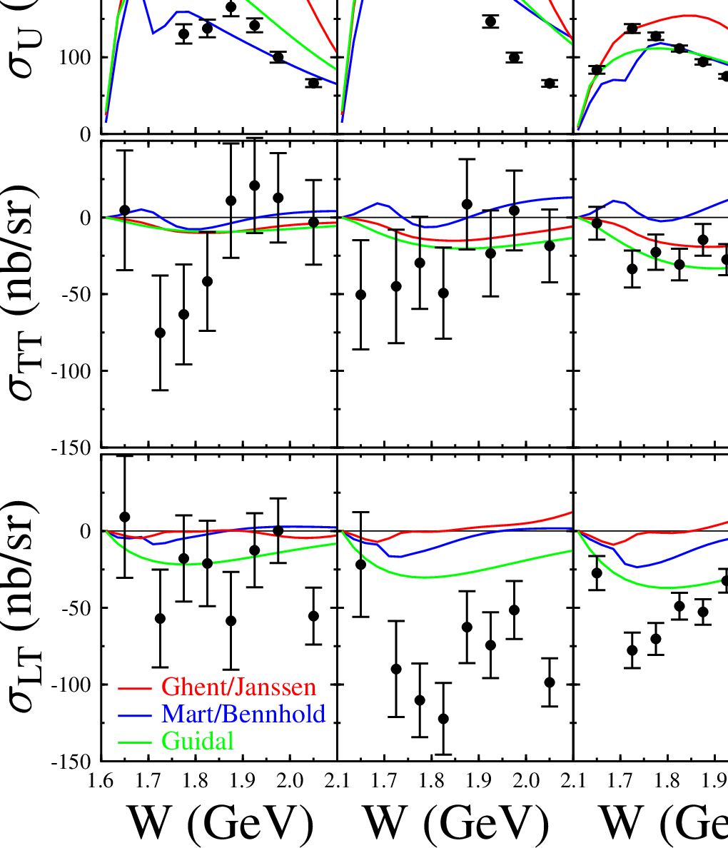
6 Electroexcitation of the $\Delta(1232)P_{33}$ , $N(1440)P_{11}$ , $N(1520)D_{13}$ , and $N(1535)S_{11}$

The new results on the electroexcitation of nucleon resonances in single pion electroproduction ( $ep\rightarrow eN\pi$ ) have been obtained mostly using the CLAS detector at JLab/Hall B (Table 1). Detailed analyses of these data sets have been performed by two groups: JLab [136, 137] and Mainz [166, 167]. The JLab analysis was carried using two approaches, DR and UIM [132, 137], and the amplitudes of the electroexcitation of the resonances $\Delta(1232)P_{33}$ , $N(1440)P_{11}$ , $N(1520)D_{13}$ , and $N(1535)S_{11}$ were obtained in the range of $Q^{2}$ covered by the CLAS data. The goal of this analysis was to determine in detail the $Q^{2}$ behavior of the resonance electrocoupling amplitudes or transition form factors. To achieve this in the least model-dependent way, the data were analyzed at each $Q^{2}$ point separately without a priori assumptions on the $Q^{2}$ dependence of the electrocoupling amplitudes. Significant effort has been put into accounting for model uncertainties and systematic uncertainties of the extracted electroexcitation amplitudes. Taken into account were uncertainties in hadronic parameters, such as masses and widths of resonances, the amplitudes of higher lying resonances, the parameters that determine the non-resonant contributions, as well as the point-to-point systematics of the experimental data and the overall normalization uncertainties of the cross sections. Utilization of two approaches, DR and UIM, also allowed the estimation of the model dependence of the results. The results of the JLab group are presented with the total model uncertainties that include all uncertainties listed above.

The analysis of the Mainz group includes, in addition to the CLAS data, backward $\pi^{0}$ electroproduction data from Hall A at $Q^{2}=1$ GeV² [5] (Table 1), and also older data from the SAID database [150] on $ep\rightarrow ep\pi^{0},en\pi^{+}$ for $W=1.1-2~$ GeV and $Q^{2}=0.1-4.4$ GeV². The analysis is based on MAID2007 [166]. A global fit of the data simultaneously at all $Q^{2}$ has been performed using parameterizations of the electroexcitation amplitudes as a function of $Q^{2}$ . In addition, for the $\Delta(1232)P_{33}$ , the electroexcitation amplitudes were constrained using theoretical predictions of Ref. [175]. All amplitudes have been constrained by the Siegert theorem [176], which gives relations between the amplitudes at the unphysical threshold when the virtual photon 3-momentum ${\bf{k}}\rightarrow 0$ . As the result of the global fit, parameterizations of the helicity amplitudes were obtained not only for the resonances of the first and second resonance regions, but also for the resonances of the third resonance region; the latter results will be discussed in section 7.

The $\Delta(1232)P_{33}$ electroexcitation amplitudes found in the MAMI ( $Q^{2}=0.06,0.2~$ GeV²) [22, 23, 24], MIT/Bates ( $Q^{2}=0.127~$ GeV²) [28, 29, 30], JLab Hall A ( $Q^{2}=1~$ GeV²) [6, 7] and Hall C ( $Q^{2}=2.8,4.2~$ GeV²) [18] experiments on $ep\rightarrow ep\pi^{0}$ will be presented according to discussions in sections 5.1.2-5.1.4. We also present the amplitudes of the transitions $\gamma^{*}p\rightarrow N(1535)S_{11}$ and $\gamma^{*}p\rightarrow N(1440)P_{11}$ and $N(1520)D_{13}$ found, respectively, from the $\gamma^{*}p\rightarrow\eta p$ and $\gamma^{*}p\rightarrow\pi\pi N$ reactions. The methods used for the extraction of the resonance contributions in these processes are described in sections 5.3 and 5.4.

6.1 The $\Delta(1232)P_{33}$ resonance

Historically, the electromagnetic transition amplitudes for the $\Delta(1232)P_{33}$ have been presented in terms of the $\gamma^{*}N\rightarrow\Delta(1232)P_{33}$ magnetic-dipole transition form factor and the ratios $R_{EM}$ and $R_{SM}$ . For the $\gamma^{*}N\rightarrow\Delta(1232)P_{33}$ magnetic-dipole transition form factor we use the Ash convention [177], which relates $G^{*}_{M,Ash}(Q^{2})$ to the multipole amplitude $M_{1+}^{3/2}(Q^{2},W)$ at the resonance position in the following way:

G^{*}_{M,Ash}(Q^{2})=\frac{m}{k_{r}}\sqrt{\frac{8q_{r}\Gamma}{3\alpha}}M_{1+}^{3/2}(Q^{2},W=M),

(111)

where $M=1232~$ MeV and $\Gamma=118$ MeV are the mass and width of the $\Delta(1232)P_{33}$ , $q_{r},k_{r}$ are the pion and virtual photon three-momenta, respectively, in the c.m.s. of the reaction $\gamma^{*}p\rightarrow p\pi^{0}$ at the $\Delta(1232)P_{33}$ resonance position, and $m$ is the nucleon mass. The Jones-Scadron convention [108], which is also used, is related to $G^{*}_{M,Ash}$ as:

G^{*}_{M,J-S}(Q^{2})=G^{*}_{M,Ash}(Q^{2})\sqrt{1+\frac{Q^{2}}{(M+m)^{2}}}.

(112)

The results for $G^{*}_{M,Ash}(Q^{2})$ , $R_{EM}$ , and $R_{SM}$ extracted from experiments are shown in Fig. 28. For $G^{*}_{M,Ash}(Q^{2})$ , we also include the results of earlier experiments from NINA [185] and DESY [186, 187]. The earlier results for $R_{EM}$ and $R_{SM}$ had large uncertainties and are not shown. In the recent experiments, the $Q^{2}$ range is significantly enlarged, and accurate results are obtained for all quantities $G^{*}_{M}(Q^{2})$ , $R_{EM}$ and $R_{SM}$ .

6.1.1 On the JLab and MAID2007 results

The JLab and MAID2007 results for the magnetic-dipole transition form factor and for $R_{EM}$ are in good agreement with each other. The latter is consistent with a constant value; its averaged value in the range $0<Q^{2}<7$ GeV² is $R_{EM}=-2.11\pm 0.06\%$ . However, there are significant differences in the results for $R_{SM}$ , especially at large $Q^{2}$ . We address this discrepancy as it has led to confusion regarding the scale of $Q^{2}$ where the asymptotic QCD behavior may set in for the transition $\gamma^{*}N\rightarrow\Delta(1232)P_{33}$ .

The magnitude of the relevant amplitude $S_{1+}^{3/2}$ can be checked using the experimentally determined structure function $\sigma_{LT}(ep\rightarrow ep\pi^{0})$ , whose $\cos{\theta}$ behavior at $W=1.232~$ GeV is dominated by the interference of this amplitude with $M_{1+}^{3/2}$ (see Eq. (101)). The comparison of the experimental data for the $ep\rightarrow ep\pi^{0}$ structure functions with the results of the JLab and MAID2007 solutions is shown in Figs. 11, 12, and 13. At $Q^{2}=0.4-1.45~$ GeV² (Fig. 11), the JLab and the MAID2007 solutions describe equally well the angular behavior of $\sigma_{LT}$ . However, MAID2007 analysis increasingly underestimates the strong $\cos{\theta}$ dependence of this structure function with rising $Q^{2}$ . This is a direct consequence of the small magnitude of $R_{SM}$ in the MAID2007 solution. At $Q^{2}\geq 3$ GeV² this is demonstrated in Figs. 12 and 13.

6.1.2 CQM and pion-cloud contribution

It is well known that the prediction of the $\gamma N\rightarrow\Delta(1232)P_{33}$ transition magnetic moment was one of the first successes of the constituent quark model [193]. The assumption that the nucleon and the $\Delta(1232)$ consist of three constituent quarks moving non-relativistically in an $s$ -wave led to the prediction

\mu(\gamma p\rightarrow\Delta)=\frac{2\sqrt{2}}{3}\mu_{p},~~i.e.~~\mu(\gamma p\rightarrow\Delta)=2.63\frac{e}{2m},

(113)

where $\mu(\gamma p\rightarrow\Delta)$ is related to the $\gamma N\rightarrow\Delta(1232)P_{33}$ magnetic-dipole form factor as [194]:

\mu(\gamma p\rightarrow\Delta)=\frac{e}{2m}\frac{2M}{M+m}G^{*}_{M,Ash}(Q^{2}=0).

(114)

Another prediction, which is a direct result of this assumption, is that the electric-quadrupole and scalar quadrupole $\gamma N\rightarrow\Delta(1232)P_{33}$ transitions are forbidden [195, 196]:

R_{EM}(Q^{2})=R_{SM}(Q^{2})=0.

(115)

This follows from angular momentum conservation: the corresponding photons carry total angular momentum $J_{\gamma}=2$ and, therefore, cannot be absorbed by quarks in an $s$ -wave. Qualitatively these predictions are in good agreement with experiment and are considered as a success of the constituent quark model, although the predicted value of $\mu(\gamma p\rightarrow\Delta)$ (Eq. (113)) underestimates the experimental results [194, 197]. With the amplitudes $A_{1/2}$ and $A_{3/2}$ at $Q^{2}=0$ quoted by RPP [174], one obtains

	$\displaystyle G^{*}_{M}(0)=3.02\pm 0.03,$		(116)
	$\displaystyle\mu(\gamma p\rightarrow\Delta)=[3.44\pm 0.03]\frac{e}{2m}.$		(117)

The non-relativistic quark model prediction is below the experimental value by about 30%. Moreover, experiments also give non-zero values for $R_{EM}$ and $R_{SM}$ . Despite a large effort to improve the agreement with experiment through modifications of the CQM with different schemes of relativization, configuration mixings in $N$ and $\Delta$ , and the inclusion of quark anomalous magnetic moments, no significant progress in the description of the $\gamma N\rightarrow\Delta(1232)P_{33}$ transition magnetic moment was achieved within constituent quark model. A satisfactory description of $\mu(\gamma p\rightarrow\Delta)$ was achieved in the models that include pion-cloud contribution: the cloudy bag model [37], the chiral bag model [39], and the Lorentz covariant chiral quark model [40]. The models of Refs. [37, 40] gave also non-zero values of the ratios $R_{EM}$ and $R_{SM}$ , which are quite close to the experimental data. The chiral chromodielectric and $\sigma$ models of Ref. [38], that include pion-cloud contribution, give non-zero values of the ratios $R_{EM}$ and $R_{SM}$ too. In Refs. [37, 38], these ratios are determined almost completely by the pion-cloud contributions. The predictions of Ref. [38] extend up to $Q^{2}=1~$ GeV² and are shown in Fig. 29.

Non-zero values of the ratios $R_{EM}$ and $R_{SM}$ are obtained also in the constituent quark model with the inclusion of two-body exchange currents that may be associated with the cloud of quark-antiquark pairs [175, 188, 189, 190]. The obtained ratio $R_{EM}(0)$ receives sizeable contribution from exchange currents and is quite close to the experimental value. The prediction for $R_{SM}$ is:

R_{SM}(Q^{2})=\frac{mk_{r}}{2Q^{2}}\frac{G_{C}^{n}(Q^{2})}{G_{M}^{n}(Q^{2})},

(118)

where $G_{C}^{n}(Q^{2})$ and $G_{M}^{n}(Q^{2})$ are the neutron charge and magnetic form factors. The results that follow from Eq. (118) for two different parameterizations of the neutron charge form factor are shown in Fig. 29. It can be seen that the approach describes the sign and order of magnitude of the ratio $R_{SM}$ extracted from experimental data.

The contributions of the quark core and meson cloud to $\gamma N\rightarrow\Delta(1232)P_{33}$ can be separated within dynamical reaction models. One may expect that the quark core contribution can be identified in these models with the ‘bare’ resonance contribution, while the meson-cloud effects correspond to the $t$ -channel meson exchanges followed by the $\pi N$ rescattering. The total $\gamma N\rightarrow\Delta(1232)P_{33}$ amplitude corresponds to the ‘dressed’ resonance. Fig. 28 shows the ‘bare’ and ‘dressed’ resonance contributions to $G^{*}_{M,Ash}(Q^{2})$ , $R_{EM}$ , and $R_{SM}$ obtained in the SL dynamical model [45] through the description of the experimental data on $ep\rightarrow ep\pi^{0}$ at $Q^{2}<4$ GeV². The corresponding results of the DMT dynamical model [43, 44] are very similar to those obtained by SL. The pion-cloud contribution is significant and accounts for more than 30% of $G^{*}_{M,Ash}(Q^{2})$ at the photon point and remains sizable even at large $Q^{2}$ . As in the models [37, 38], the $R_{EM}$ and $R_{SM}$ ratios of the dynamical models [43, 44, 45] are almost exclusively determined by the meson-cloud contributions.

6.1.3 Perturbative QCD asymptotic limits

The asymptotic limit of pQCD puts restrictions on the $Q^{2}$ behavior of the $\gamma^{*}N\rightarrow N^{*}$ transition amplitudes that follow from hadron helicity conservation [74] and dimensional counting rules [75, 76, 77, 78, 79]. These restrictions are specific to the hard scattering mechanism when large transferred momentum is shared among the three quarks through two hard gluon exchanges (Fig. 30). Below we discuss in more detail the predictions for the helicity amplitudes $A_{1/2}$ , $A_{3/2}$ , and $S_{1/2}$ . Following the discussion in Ref. [198], we consider the $\gamma^{*}N\rightarrow N^{*}$ transition in the Breit system, where

{\bf p}=-{\bf p^{*}};{\bf k}=-2{\bf p}.

(119)

From relativistic invariance it follows that the matrix elements entering Eqs. (31-33) can be written in the Breit frame in the following way:

<N^{*},S_{z}^{*}|\epsilon^{(\lambda_{\gamma})}_{\mu}J_{em}^{\mu}|N,S_{z}>=<\lambda_{N^{*}}|\epsilon^{(\lambda_{\gamma})}_{\mu}J_{em}^{\mu}|\lambda_{N}>_{Breit~frame},

(120)

where $\lambda_{N}=-S_{z}$ and $\lambda_{N^{*}}=S_{z}^{*}$ .

In the limit $Q^{2}\rightarrow\infty$ , we have $|{\bf p}|\simeq|{\bf p^{*}}|\sim\frac{Q}{2}$ ; therefore, the $N$ and $N^{*}$ masses, and also the quark masses and transverse momenta, can be neglected compared to their longitudinal momenta. In this case, the gluon and photon interaction vertices with quarks ( $\gamma_{\mu}$ ) preserve the quark helicity, and every quark that requires its helicity to be flipped introduces an additional factor $\sim 1/Q$ . For the matrix elements that enter Eqs. (31,32,33) we have, respectively, $\lambda_{N^{*}}-\lambda_{N}=0,2,1$ . Therefore:

\tilde{A}^{N}_{3/2}/\tilde{A}^{N}_{1/2}\sim 1/Q^{2},~~~~~\tilde{A}^{N}_{1/2}/\tilde{S}^{N}_{1/2}\sim const.

(121)

Here, we took into account the factor $\frac{|{\bf k}|}{Q}\approx\frac{Q}{2m}$ in the definition (33) for $\tilde{S}^{N}_{1/2}$ .

Using the more detailed evaluation of the asymptotic $Q^{2}$ behavior of the helicity amplitudes in the Breit frame in Ref. [198], we get the following results:

\tilde{A}^{N}_{1/2}\sim 1/Q^{3},~~~~~\tilde{A}^{N}_{3/2}\sim 1/Q^{5},~~~~~\tilde{S}^{N}_{1/2}\sim 1/Q^{3}.

(122)

Furthermore, taking into account the definitions (5), (23-25), and (35) of section 3, we obtain the asymptotic predictions for $R_{EM}$ and $R_{SM}$ :

R_{EM}\rightarrow 100\%,~~~~R_{SM}\rightarrow const,~~~~Q^{2}\rightarrow\infty.

(123)

The study of $R_{EM}(Q^{2})$ and $R_{SM}(Q^{2})$ should give clear understanding of the $Q^{2}$ range where the pQCD regime for the $\gamma N\rightarrow\Delta(1232)P_{33}$ transition may set in.

The results for $R_{EM}(Q^{2})$ and $R_{SM}(Q^{2})$ extracted from experimental data show that $R_{EM}$ remains negative, small, and nearly constant in the entire range $0<Q^{2}<7$ GeV²; $R_{SM}$ remains negative, but its magnitude strongly rises at high $Q^{2}$ . Consequently, there is no indication that asymptotic pQCD is applicable in the range $0<Q^{2}<7~$ GeV² covered by experiment. The very small value of $R_{EM}$ at the highest $Q^{2}$ values indicates that there is not even a trend towards that limit.

It should be mentioned however, that the asymptotic behaviour given by Eqs. (121,122,123) corresponds to the inner part of the hard scattering diagram of Fig. 30, i.e. to the part related to the quarks only. Higher order corrections and convolution with the soft $N$ and $N^{*}$ distribution amplitudes may introduce logarithmic corrections. The convolution is needed also to calculate numerical coefficients in Eqs. (121,122,123). In Ref. [198], for example, it is shown that the asymptotic form of nucleon wave function suggested in Ref. [199] results in significant destructive interference between contributions related to different parts of this wave function. This can strongly suppress the $\gamma N\rightarrow\Delta(1232)P_{33}$ amplitude in the pQCD limit.

For the ratio $R_{SM}$ , logarithmic corrections caused by the orbital motion of the constituents in the nucleon and the $\Delta(1232)P_{33}$ are found in Ref. [191]:

R_{SM}=c\frac{|{\bf k}|}{Q^{2}}ln^{2}(Q^{2}/\Lambda^{2}),

(124)

where $c$ is an unknown factor, and $\Lambda=0.2\div 0.4$ is a soft scale related to the size of hadrons. Corresponding results with $\Lambda=0.2$ that gives maximal slope for $R_{SM}$ are shown in Fig. 29. The coefficient $c$ has been found from the data at $Q^{2}=2.8\div 4.2~$ GeV². It can be seen that logarithmic corrections are not sufficient to describe strongly rising magnitude of $R_{SM}$ found in experiment.

To conclude this section, we would like to mention the results obtained in Ref. [192]. The investigation exploits the observation of Refs. [200, 201] that the experimental data on the ratio of the nucleon form factors $F_{1}(Q^{2})$ and $F_{2}(Q^{2})$ [202, 203] exhibit the pQCD scaling behaviour starting with small $Q^{2}=0.5-1~$ GeV², while the form factors themselves do not. Good description of this ratio has been obtained due to the logarithmic corrections found in Ref. [200]. On this basis in Ref. [192], a phenomenological multi-parameter approach was proposed to describe the ratios $R_{EM}$ and $R_{SM}$ . With the parameters found from the fit to the data at $Q^{2}<7~$ GeV², the extension was made to higher $Q^{2}$ . According to the results shown in Fig. 29, $R_{SM}$ will continue to grow in magnitude, while $R_{EM}$ will cross zero around $Q^{2}=5$ GeV² and become positive. While the Jlab data disfavor this prediction for $R_{EM}$ , a zero-crossing at somewhat higher $Q^{2}$ values is not excluded taking into account statistical and systematic uncertainties of the $R_{EM}$ values extracted from experiment. These results can be checked in future JLab experiments at 12 GeV.

6.1.4 Large $N_{c}$ limit and GPDs

It is well known that in the limit of a large number of colors, $N_{c}$ , many results of the $SU(6)$ symmetric quark model can be obtained without making model assumptions. For example, in that limit we have: ${\mu_{p}}/{\mu_{n}}=-\frac{3}{2}$ , i.e. the same result as in the non-relativistic quark model. The prediction for the $\gamma N\rightarrow\Delta(1232)P_{33}$ magnetic moment is [204]:

\mu(\gamma p\rightarrow\Delta)=\frac{1}{\sqrt{2}}(\mu_{p}-\mu_{n}).

(125)

This gives $\mu(\gamma p\rightarrow\Delta)=3.23\frac{e}{2m}$ , which is very close to the experimental value (Eq. 117). The predictions for $R_{EM}(0)$ and $R_{SM}(0)$ in the large $N_{c}$ limit with $M=m$ are $R_{EM}(0)=R_{SM}(0)=0$ [54, 55, 205], i.e. the same as in the non-relativistic quark model (Eq. 115). With empirical masses ( $M-m\neq 0$ ), there are two kinds of predictions for $R_{EM}(0)$ and $R_{SM}(0)$ :

R_{EM}(0)=R_{SM}(0)=\frac{1}{12}\left(\frac{m}{M}\right)^{3/2}(M^{2}-m^{2})\frac{r_{n}}{\kappa_{V}}

(126)

and

R_{EM}(0)=R_{SM}(0)=-\frac{M-m}{3M+m},

(127)

where $r_{n}$ is the neutron charge radius and $\kappa_{V}=\frac{2m}{e}(\mu_{p}-\mu_{n})$ . Eqs. (126) are derived in Ref. [54] using the relation between the $N\rightarrow\Delta$ quadrupole moment and $r_{n}$ found in the large $N_{c}$ limit in Ref. [205]. Eqs. (127) are obtained in Ref. [55] in the approach based on the conjunction of large $N_{c}$ QCD with the idea of holography.

Numerically the relations (126) and (127) give, respectively,

R_{EM}(0)=R_{SM}(0)=-2.77\%

(128)

and

R_{EM}(0)=R_{SM}(0)=-6.3\%.

(129)

Therefore, with empirical masses $M$ and $m$ , the ratios $R_{EM}(0)$ and $R_{SM}(0)$ gain correct signs in both approaches [54] and [55]; with this the predictions for $R_{EM}$ (126,128) and $R_{SM}$ (127,129) are close to the experimental values:

	$\displaystyle R_{EM}=-(2.5\pm 0.5)\%~~(Q^{2}=0)~~\cite[cite]{[\@@bibref{}{PDG}{}{}]},$		(130)
	$\displaystyle R_{SM}=-(4.81\pm 0.27\pm 0.26)\%~~(Q^{2}=0.06~\rm{GeV}^{2})~~\cite[cite]{[\@@bibref{}{Stave2008}{}{}]}.$		(131)

In Ref. [54], the relations (126) are extended to finite values of $Q^{2}$ via parameterizations:

	$\displaystyle R_{EM}=-\left(\frac{m}{M}\right)^{3/2}\frac{M^{2}-m^{2}}{2Q^{2}}\frac{G_{En}(Q^{2})}{F_{2p}(Q^{2})-F_{2n}(Q^{2})},$		(132)
	$\displaystyle R_{SM}=-\left(\frac{m}{M}\right)^{3/2}\frac{\sqrt{[(M+m)^{2}+Q^{2}][(M-m)^{2}+Q^{2}]}}{2Q^{2}}\frac{G_{En}(Q^{2})}{F_{2p}(Q^{2})-F_{2n}(Q^{2})},$		(133)

where $F_{2N}(Q^{2})$ is the nucleon Pauli form factor and $G_{En}(Q^{2})$ is the neutron electric form factor. We note that in this parameterization $R_{EM}$ and $R_{SM}$ have the same dependence on the nucleon form factors. Hence, the double ratio $R_{SM}/R_{EM}$ depends only on kinematical quantities. The relations (132,133) give a reasonably good description of the experimental data for $Q^{2}<1.5~$ GeV². The corresponding results are shown in Fig. 28.

The generalization of the predictions (127) to $Q^{2}\neq 0$ is obtained in Ref. [55] in the leading order over $1/N_{C}$ :

	$\displaystyle R_{EM}=-\frac{M^{2}-m^{2}-Q^{2}}{(3M+m)(M+m)+Q^{2}},$		(134)
	$\displaystyle R_{SM}=-\frac{\sqrt{4M^{2}Q^{2}+(M^{2}-m^{2}-Q^{2})^{2}}}{(3M+m)(M+m)+Q^{2}}.$		(135)

Both ratios have the correct pQCD behavior. With this it is remarkable that at $Q^{2}\rightarrow\infty$ , $R_{SM}\rightarrow-100\%$ . Such asymptotic value of $R_{SM}$ might be expected taking into account the rapidly rising magnitude and negative value of $R_{SM}$ found experimentally (Fig. 28). In Fig. 28, we show also the prediction for the magnetic-dipole $\gamma p\rightarrow\Delta$ transition obtained in the same Ref. [55]. The description at $Q^{2}>0.5$ GeV² is quite satisfactory. The disagreement at small $Q^{2}$ may be attributed to the lack of higher $1/N_{c}$ corrections in the calculations.

The prediction (125) for the magnetic-dipole $\gamma p\rightarrow\Delta$ transition was extended in Ref. [53] to finite values of $Q^{2}$ . This was made by utilizing the GPD formalism, a recently developed framework that utilizes hard exclusive processes to determine spin-dependent and spin-independent leading twist amplitudes which characterize the 3-dimensional internal structure of the nucleon and of the transitions like $N\rightarrow\Delta$ (see, for example, reviews [206, 207]). The relation between the $N\rightarrow\Delta$ GPD $H_{M}$ and the nucleon isovector GPD $E^{u}-E^{d}$ in the large $N_{c}$ limit is derived in Refs. [206, 208]:

H_{M}(x,\xi,Q^{2})=2\frac{G_{M}^{*}(0)}{\kappa_{V}}[E^{u}(x,\xi,Q^{2})-E^{d}(x,\xi,Q^{2})].

(136)

Using this relation in Ref. [53], the following sum rule was found:

	$\displaystyle G^{*}_{M,J-S}(Q^{2})$		$\displaystyle=\frac{G_{M}^{*}(0)}{\kappa_{V}}\int^{+1}_{-1}dx[E^{u}(x,\xi,Q^{2})-E^{d}(x,\xi,Q^{2})]$		(137)
			$\displaystyle=\frac{G_{M}^{*}(0)}{\kappa_{V}}[F_{2p}(Q^{2})-F_{2n}(Q^{2})].$		(137)

Furthermore, with the Regge parameterization of GPDs suggested in Ref. [209], a good description of the magnetic-dipole $\gamma p\rightarrow\Delta$ transition was obtained up to $Q^{2}=8~$ GeV² [53]. This result is presented in Fig. 28.

6.1.5 Lattice QCD

The first lattice QCD study of the $\gamma p\rightarrow\Delta$ transition was carried out in Ref. [210] in the quenched approximation and with limited statistics. Negative values were obtained for both $R_{EM}$ and $R_{SM}$ ; however, because of large statistical uncertainties, a zero value could not be excluded for either of these ratios. Increased statistics, and a number of improvements introduced later, allowed the evaluation of the $\gamma p\rightarrow\Delta$ form factors with better accuracy [41, 56, 211, 212]. The results obtained in Ref. [211] in the quenched approximation and linearly extrapolated to the physical pion mass are shown in Fig. 31. A non-zero value with the correct sign was obtained for $R_{EM}$ . $R_{SM}$ is in good agreement with the experimental results in the entire $Q^{2}$ range covered by the calculations, with the exception of small $Q^{2}$ . At $Q^{2}<0.4$ GeV², the lattice results are negative but smaller in magnitude than the experimental values. The first calculations with dynamical quarks were performed in Ref. [41]. The results that correspond to the lowest pion mass $m_{\pi}=350$ MeV are shown in Fig. 31. For the ratios $R_{EM}$ and $R_{SM}$ , they confirm non-zero and negative values obtained in the quenched approximation. For $R_{SM}$ at small $Q^{2}$ , the unquenched calculations show a slightly decreasing gap between the lattice results and experiment.

For the magnetic-dipole form factor, unquenched calculations give better agreement with experiment. However, a complete description is not achieved in spite of a quite small pion mass. In Ref. [41], the conclusion is made that the most likely source for this disagreement is the fact that pion masses are still too large.

6.2 The Roper resonance: $N(1440)P_{11}$

The results for the $\gamma^{*}p\rightarrow N(1440)P_{11}$ helicity amplitudes are presented in Fig. 32. The CLAS measurements allowed for the first time the determination of the electroexcitation amplitudes for this resonance at $Q^{2}>0$ in the range $Q^{2}<4.5~$ GeV². The amplitudes are extracted from CLAS $\pi$ and 2 $\pi$ electroproduction data, both of which are sensitive to the $N(1440)P_{11}$ contribution owing to the large branching ratios of this resonance to the $\pi N$ and $2\pi N$ channels. The amplitudes extracted from the two channels are in good agreement with each other, thus confirming the reliability of the obtained results, as the non-resonant contributions and resonance decay mechanisms are different in these reactions. Within uncertainties, the results of the JLab and Mainz analyses of pion electroproduction data are also in good agreement with each other.

6.2.1 The Roper resonance: a predominantly first radial excitation of the $3q$ ground state

The so-called Roper resonance, $N(1440)P_{11}$ , is the lowest excited state of the nucleon. In the CQM, the simplest and most natural assumption is that this resonance is the first radial excitation of the three quark ( $3q$ ) ground state and belongs to the multiplet $[56,0^{+}]_{r}$ . However, the first calculations within the non-relativistic CQM with the oscillator potential failed to reproduce the mass and width of the resonance (see Ref. [60] and numerous references therein). Moreover, the oscillator potential led to the wrong mass ordering between the Roper resonance and the resonances of the multiplet $[70,1^{-}]$ , in particular, the $N(1535)S_{11}$ . It was realized later [214] that the sign of the $\gamma^{*}p\rightarrow~N(1440)P_{11}$ transition amplitude at the photon point is also not consistent with the non-relativistic CQM. These discrepancies made the state a problematic object for the CQM.

Further investigations provided better results. Estimations of the mass in the relativized quark model with more realistic potential motivated by QCD significantly reduced the difference of the computed and empirical mass from initially $\sim 600~$ MeV to $\sim 100~$ MeV [60, 217]. The quark models, where the quarks were assumed to interact by Goldstone boson exchanges, gave the correct mass ordering between the $N(1440)P_{11}$ and $N(1535)S_{11}$ [218]. The description of the width was also improved. In the quark model that incorporates some of the features expected from QCD, the gap between the empirical width and theoretical calculations was significantly reduced [92]; a good description of the width was obtained within the pair-creation ${}^{3}P_{0}$ model [61, 219, 220]. The LF relativistic quark model gave the correct sign of the $\gamma^{*}p\rightarrow~N(1440)P_{11}$ amplitude at the photon point [214].

In spite of the positive developments in the CQM, the Roper resonance continued to be considered as a ‘puzzle’ and gave rise to the attempts to describe this resonance in alternative approaches or by complementing the $3q$ state with $qqqq\bar{q}$ components. The electroexcitation amplitudes of the Roper resonance were evaluated assuming this resonance has a gluonic component in its wave function, i.e. it is a hybrid state $q^{3}G$ [66, 67]. Such an approach was motivated by the fact that in the bag model, the lightest hybrid state has quantum numbers of the Roper resonance, and its mass can be $<1.5~$ GeV [68]. The helicity amplitudes $A_{1/2}(Q^{2})$ and $S_{1/2}(Q^{2})$ predicted in the hybrid model were consistent with the early data that showed the rapid disappearance of $A_{1/2}$ with $Q^{2}$ and $S_{1/2}(Q^{2})\sim 0$ . Also suggested were alternative descriptions of the $N(1440)P_{11}$ as a $N\sigma$ molecule [221, 222] or a dynamically generated resonance [223]. The empirical width of the $N(1440)P_{11}$ was described within the non-relativistic CQM by complementing the $3q$ state with a $30\%$ $qqqq\bar{q}$ component [62].

The CLAS measurements made possible, for the first time, the determination of the electroexcitation amplitudes of the Roper resonance on the proton in a wide range of $Q^{2}$ . These results are crucial to get a better understanding of the nature of this state. Fig. 32 shows that the transverse helicity amplitude $A_{1/2}$ of the $\gamma^{*}p\rightarrow N(1440)P_{11}$ transition extracted from CLAS data exhibits a very specific behavior. This amplitude, being large and negative at $Q^{2}=0$ , changes sign in the range $0.4<Q^{2}<0.65~$ GeV², and becomes large and positive at $Q^{2}>1.5~$ GeV². With increasing $Q^{2}$ , $A_{1/2}$ drops smoothly in magnitude. Such a behaviour is qualitatively reproduced by the LF relativistic quark models [214, 215, 224, 225, 226] assuming that the Roper resonance $N(1440)P_{11}$ is the first radial excitation of the $3q$ ground state. The results obtained in these models are presented and reviewed in Ref. [215]. In Fig. 32, we show the predictions [215], which extend over the full $Q^{2}$ range investigated in experiment. Under the assumption that the Roper resonance is a first radial excitation of the $3q$ ground state, the LF relativistic quark models also describe the sign of the longitudinal $\gamma^{*}p\rightarrow N(1440)P_{11}$ amplitude. Under the same assumption, a good description of both amplitudes at high $Q^{2}$ is obtained within the covariant quark model of Ref. [216].

The LF relativistic quark models [214, 215, 224, 225, 226] and the approach of Ref. [216] fail, however, to describe the data at small $Q^{2}$ . This can have a natural explanation in the meson-cloud contribution. Indeed, the description at small $Q^{2}$ is significantly improved [227, 228] when a quark core, taken as the first radial excitation of the $3q$ ground state, is combined with a meson cloud. The last contribution is constructed in the approaches [227, 228] in different ways. In Ref. [227], the meson-cloud contribution is found in the pair-creation ${}^{3}P_{0}$ model, while in Ref. [228] it corresponds to the $N+\sigma$ contribution. It should be mentioned that the strong $N+\sigma$ content is found in the Roper resonance via estimations in a gluon exchange model [222], and also in the analysis of data on pion- and photon-induced reactions [229]. A large meson-cloud contribution to $A_{1/2}$ is expected also according to the coupled-channel analysis of pion photoproduction data [159].

An important aspect of the transition amplitudes is their signs. As we discussed in section 3.3, the experimental results on the $\gamma^{*}N\rightarrow~N^{*}$ amplitudes, extracted from the contribution of diagram (d) in Fig. 4 to $\gamma^{*}N\rightarrow~N\pi$ , contain the sign of the hadronic $\pi NN^{*}$ vertex. The sign of the $N(1440)P_{11}\rightarrow\pi N$ vertex was first found in Ref. [214] using the ${}^{3}P_{0}$ model, and confirmed by a computation using the LF relativistic quark model [215]. A comparison between the empirical amplitudes and the quark model predictions is given in Figs. 32 and 33 taking into account this sign.

Here we briefly comment on the sign of the $\gamma^{*}p\rightarrow~N(1440)P_{11}$ amplitudes in the non-relativistic quark models. Traditionally, the sign of $A_{1/2}(Q^{2}=0)$ has been fixed to the experimentally determined sign of that amplitude at $Q^{2}=0$ . In this case, the non-relativistic quark model predictions for both amplitudes $A_{1/2}$ and $S_{1/2}$ have negative signs. As examples, we refer to the predictions from Ref. [67]. The negative signs of $A_{1/2}$ and $S_{1/2}$ are in contradiction to the experimental data: for $S_{1/2}$ at all $Q^{2}$ , and for $A_{1/2}$ at $Q^{2}>0.5$ GeV². They also contradict the LF relativistic quark model predictions. However, if we take into account the sign of the $N(1440)P_{11}\rightarrow\pi N$ vertex found in Refs. [214, 215], the non-relativistic quark model predictions for the $\gamma^{*}p\rightarrow~N(1440)P_{11}$ amplitudes get signs opposite to those found in the traditional way, and the aforementioned disagreement disappears (see the results from Ref. [67] presented in Fig. 32 with the correct signs).

Taken together, the arguments presented above provide strong evidence in favor of the Roper resonance $N(1440)P_{11}$ as predominantly the first radial excitation of the $3q$ ground state.

In Fig. 32, we present the predictions obtained assuming that the Roper resonance is a hybrid state [66, 67]. They definitely contradict the amplitudes extracted from experimental data. It is important to mention that although the suppression of the longitudinal amplitude $S_{1/2}$ is obtained in Refs. [66, 67] up to $O(v^{2}/c^{2})$ , it has a physical origin, which makes this result practically independent of relativistic effects. The presentation of the $N(1440)P_{11}$ as a $q^{3}G$ hybrid state is definitely ruled out.

6.2.2 Light-front holographic QCD

Convincing arguments in favor of the point of view that the Roper resonance is a first radial excitation of the nucleon have been obtained very recently in the light-front holographic QCD [230, 231]. This approach is built on the correspondence between semiclassical QCD quantized on the light-front and a dual gravity model in anti-de Sitter (AdS) space providing an approximation to QCD in its strongly coupled regime. The arguments are based on the description of the mass of the Roper resonance and the $F_{1}(Q^{2})\equiv Q^{2}G_{1}(Q^{2})$ form factor for the $\gamma^{*}p\rightarrow~N(1440)P_{11}$ transition (see definitions (3.4,43)).

Using Schrödinger and Dirac equations with a linear confining potential and fixing the overall energy scale to be identical for mesons and baryons, the masses of mesons and baryons on the Regge trajectories that correspond to $\pi,\rho,\omega$ , and positive parity baryon states are derived. These masses are consistent with the empirically observed masses. The Roper resonance $N(1440)P_{11}$ and the $N(1710)P_{11}$ are well accounted in this scheme as the first and second radial states of the nucleon family, likewise the $\Delta(1600)P_{33}$ corresponds to the first radial excitation of the $\Delta$ family.

The $F_{1}(Q^{2})$ form factor is predicted without free parameters as:

F_{1}(Q^{2})=\frac{\sqrt{2}}{3}\frac{\frac{Q^{2}}{M_{\rho}^{2}}}{\left(1+\frac{Q^{2}}{M_{\rho}^{2}}\right)\left(1+\frac{Q^{2}}{M_{\rho^{\prime}}^{2}}\right)\left(1+\frac{Q^{2}}{M_{\rho^{\prime\prime}}^{2}}\right)},

(138)

where $M_{\rho}$ , $M_{\rho^{\prime}}$ , and $M_{\rho^{\prime\prime}}$ are masses of the $\rho$ meson and its first two radial states. The results are shown in Fig. 34 and are in good agreement with experimental data.

6.2.3 Lattice QCD

The electromagnetic transitions from the nucleon’s ground state to the excited states of the nucleon have not been studied in lattice QCD until very recently. The first attempts to evaluate the $\gamma^{*}p\rightarrow N(1440)P_{11}$ transition in lattice QCD were made in Ref. [57]. The calculations used the quenched approximation and a large pion mass of $\sim 720$ MeV. The Roper resonance is taken as the lowest excited state with the same quantum numbers and quark content as the nucleon. The results are given in terms of the form factors $F^{*}_{1,2}(Q^{2})$ that are related to the form factors $G_{1,2}(Q^{2})$ defined in Sec. 3.4 (Eqs. (3.4,43)) by

F^{*}_{1}(Q^{2})=Q^{2}G_{1}(Q^{2}),~~~~F^{*}_{2}(Q^{2})=-\frac{M^{2}-m^{2}}{2}G_{2}(Q^{2}).

(139)

The lattice QCD results [57] are shown in Fig. 35 in terms of the $\gamma^{*}p\rightarrow~N(1440)P_{11}$ helicity amplitudes. The signs of the amplitudes and orders of magnitudes are correctly predicted. There are obvious discrepancies at the quantitative level, especially at low $Q^{2}$ . These are not unexpected given the large pion mass and the use of the quenched approximation. As we discussed in the previous section, the pion-cloud contributions are expected to be large at small $Q^{2}$ .

6.3 The $N(1535)S_{11}$ resonance

6.3.1 JLab data on $ep\rightarrow e\pi N,e\eta p$ and determination of the branching ratios $N(1535)S_{11}\rightarrow\pi N,~\eta N$

The $N(1535)S_{11}$ resonance has large couplings to both the $\pi N$ and $\eta N$ channels and has been extensively studied in $\pi$ and $\eta$ electroproduction off protons. In the early generations of electron beam accelerators the electroexcitation of the $N(1535)S_{11}$ was studied up to $Q^{2}=3~$ GeV² (see reviews [1, 2]). A falloff of the transverse $\gamma^{*}p\rightarrow~N(1535)S_{11}$ amplitude with $Q^{2}$ was observed that was deemed unusually slow in comparison to other resonances. However, the experimental information was scarce, and the data did not allow for definite results on the longitudinal amplitude. We should also mention that modern quark models explain the observed $Q^{2}$ dependence at least qualitatively.

Starting in 1999, rich information on the $N(1535)S_{11}$ has been obtained at JLab in a wide range of $Q^{2}$ up to $4.5$ and $7$ GeV², respectively, in $\pi$ and $\eta$ electroproduction off protons (see Fig. 36). Accurate results were obtained in both reactions for the transverse amplitude $A_{1/2}$ ; they show a consistent $Q^{2}$ slope and confirm the slow fall off with $Q^{2}$ observed in earlier experiments.

In $\eta$ electroproduction, the contribution of the $N(1535)S_{11}$ is dominant at $W<1.6~$ GeV and is extracted from the data in a nearly model-independent way. However, in the recent high statistics measurements of this channel, no explicit separation of the longitudinal and transverse terms that contribute to the cross section has been undertaken. The analyses assume that the longitudinal contribution to the total cross section is small enough to have a negligible effect on the extraction of the $A_{1/2}$ amplitude. This assumption is motivated by results of the early experiments [2].

In $\pi$ electroproduction, the longitudinal amplitude can be revealed due to an interference with other contributions, resonant and non-resonant, which is absent in $\eta$ production. Due to new $n\pi^{+}$ data, for the first time definite results were obtained for this amplitude [137, 166, 167]. Estimations based on these results confirm that the inclusion of the longitudinal component would have a slight effect on the amplitude $A_{1/2}$ extracted from $\eta$ electroproduction data [16, 17, 20]. For example, the contribution of the longitudinal amplitude found in $\pi$ electroproduction to the total cross sections shown in Fig. 21 at the $N(1535)S_{11}$ resonance position is within shown statistical and systematic errors. This means that the amplitude $A_{1/2}$ estimated at the resonance position would decrease in magnitude within half of its error. However, for accurate conclusions the analyses of complete sets of data over all angles and energies are required.

Numerical comparison of the results extracted from the $\pi$ and $\eta$ photo- and electroproduction data depends on the relation between the branching ratios to the $\pi N$ and $\eta N$ channels. Consequently, it contains an arbitrariness connected with the uncertainties of these branching ratios: $\beta_{\pi N}=0.35\div 0.55$ , $\beta_{\eta N}=0.45\div 0.6$ [174].

The accurate results on the transverse amplitudes $A_{1/2}$ found from the new $\pi$ and $\eta$ data were used in Ref. [137] to specify the relation between $\beta_{\pi N}$ and $\beta_{\eta N}$ . From the fit to these amplitudes at $0\leq Q^{2}\leq 4.5$ GeV², it was found

\frac{\beta_{\eta N}}{\beta_{\pi N}}=0.95\pm 0.03.

(140)

Furthermore, taking into account the branching ratio to the $\pi\pi N$ channel, $\beta_{\pi\pi N}=0.01\div 0.1$ [174], which accounts practically for all channels different from $\pi N$ and $\eta N$ , more accurate values of the branching ratios $\beta_{\pi N}$ and $\beta_{\eta N}$ were obtained:

	$\displaystyle\beta_{\pi N}=0.485\pm 0.008\pm 0.023,$		(141)
	$\displaystyle\beta_{\eta N}=0.460\pm 0.008\pm 0.022.$		(142)

The first uncertainty corresponds to the fit uncertainty in Eq. (140), the second one accounts for the uncertainty of $\beta_{\pi\pi N}$ . The results shown in Fig. 36 correspond to $\beta_{\pi N}=0.485,~\beta_{\eta N}=0.46$ .

6.3.2 Model predictions and the sign of the $S_{1/2}$ amplitude for $\gamma^{*}p\rightarrow N(1535)S_{11}$

Constituent quark models give the correct sign for the transverse amplitude $A_{1/2}$ taking into account the sign of the $N(1535)S_{11}\rightarrow\pi N$ vertex found in the LF relativistic quark model [233]. However, there is a large diversity among predictions of different models, which is clearly seen in the results obtained from the LF relativistic quark models of Refs. [214] and [232] (see Fig. 36). This diversity prevents us from drawing quantitative conclusions on the quark core and meson-cloud contributions by utilization of the empirical values of $A_{1/2}$ .

The CQM predictions for the longitudinal amplitude $S_{1/2}$ are positive at $Q^{2}<1$ GeV², both in the relativistic and non-relativistic approaches. This is in contradiction to the amplitudes extracted from experiment. The only possibility to reach agreement with the empirical values would be large and negative contributions produced by the meson cloud or by additional $qqqq\bar{q}$ components to the $N(1535)S_{11}$ wave function. Such information is currently not available, and definite conclusions will have to wait until results of analyses within dynamical coupled-channel approaches become available. Concerning a possible 5-quark component it was found in Ref. [63] that the most likely lowest energy configuration in the $N(1535)S_{11}$ is given by a $qqqs\bar{s}$ component. This can solve, in principle, the problem of mass ordering between the $N(1440)P_{11}$ and $N(1535)S_{11}$ , and may also explain the large branching ratio of the $N(1535)S_{11}$ to the $\eta N$ channel and recently observed large couplings to the $\phi N$ and $K\Lambda$ channels [64, 65]. However, from the results of Ref. [63], one can conclude that the 5-quark contribution to both amplitudes $A_{1/2}$ and $S_{1/2}$ is small, and would also not resolve the disagreement between experiment and models regarding the $S_{1/2}$ amplitude.

It is remarkable that the signs of both amplitudes $A_{1/2}$ and $S_{1/2}$ are described within the approach of Ref. [58]. This light-cone sum rule approach may be considered a tool to derive the $\gamma^{*}p\rightarrow N(1535)S_{11}$ amplitudes from the first principles of QCD. The $N(1535)S_{11}$ light-cone distribution amplitudes are found through lattice calculations and are used to compute the $\gamma^{*}p\rightarrow N(1535)S_{11}$ transition amplitudes by utilization of light-cone sum rules. At $Q^{2}>2$ GeV², where the approach may be applicable, there is good quantitative agreement between the predictions and the amplitudes extracted from experiment.

6.4 The $N(1520)D_{13}$ resonance

Results for the $\gamma^{*}p\rightarrow~N(1520)D_{13}$ helicity amplitudes are presented in Fig. 37. The amplitudes are extracted from CLAS data on $\pi$ and 2 $\pi$ electroproduction, which are the main channels for the investigation of the $N(1520)D_{13}$ . The precise new data enabled the determination of the $\gamma^{*}p\rightarrow N(1520)D_{13}$ transition in a wider $Q^{2}$ range, and with much higher accuracy for the transverse amplitudes compared to earlier experiments. The sensitivity of the earlier data to the $S_{1/2}$ amplitude was very limited. The CLAS data allowed this amplitude to be determined with good precision.

The signs of all three helicity amplitudes are described by quark models taking into account the signs of both vertices $\gamma^{*}p\rightarrow~N(1520)D_{13}$ and $N(1520)D_{13}\rightarrow\pi N$ , with the last one taken from the LF relativistic quark model [233]. The shapes of the amplitudes are also reproduced. However, there is a significant shortfall in the quark models with regard to the $A_{3/2}$ amplitude at $Q^{2}<2$ GeV², which again may hint at large meson-cloud contributions. A coupled-channel analysis of pion photoproduction data indeed shows large meson-cloud contributions to $A_{3/2}$ [159], which could explain this discrepancy. The data show a clear dominance of the $A_{3/2}$ amplitude at the photon point. With increasing $Q^{2}$ , this amplitude drops rapidly, and its magnitude is smaller than the magnitude of $A_{1/2}$ at $Q^{2}>0.6$ GeV². In fact, $A_{1/2}$ dominates the resonance strength at high $Q^{2}$ . This is demonstrated in Fig. 38 in terms of the helicity asymmetry. The “helicity switch” was predicted in the nonrelativistic quark model with a harmonic oscillator potential [237]. It is interesting that in spite of possible large meson-cloud contributions, the empirical amplitudes reveal a behavior that is qualitatively consistent with the prediction of the naive constituent quark model.

6.5 Helicity amplitudes and the pQCD asymptotic behavior

Using the helicity amplitudes for the three excited states $N(1440)P_{11}$ , $N(1535)S_{11}$ , and $N(1520)D_{13}$ , one can check the $1/Q^{3}$ scaling prediction of pQCD for the $A_{1/2}$ and $S_{1/2}$ amplitudes. As we discussed in Sec. 6.1.3, such scaling is expected in the asymptotic limit of pQCD (see Eqs. (122)). Figs. 39 and 40 show the helicity amplitudes $A_{1/2}$ and $S_{1/2}$ multiplied by $Q^{3}$ . We note that starting with $3~$ GeV² for $A_{1/2}$ and $1.5-2~$ GeV² for $S_{1/2}$ , the empirical amplitudes show a $Q^{2}$ trend close to the expected $1/Q^{3}$ dependence, although measurements at higher $Q^{2}$ are needed for more definite conclusions.

6.6 Empirical transverse charge densities in the $\gamma^{*}p\rightarrow\Delta(1232)P_{33}$ , $N(1440)P_{11}$ , $N(1535)S_{11}$ , and $N(1520)D_{13}$ transitions

The precise results on the amplitudes of the resonance transitions $\gamma^{*}p\rightarrow~\Delta(1232)P_{33}$ , $N(1440)P_{11}$ , $N(1535)S_{11}$ , and $N(1520)D_{13}$ provide the basis needed to study the spatial characteristics of excited nucleon states. A proper density interpretation of the empirical amplitudes is obtained in Refs. [80, 81, 82] in a frame where the baryons have a large momentum-component along the $z$ -axis chosen along the direction of $\bf{P}$ ( $P=\frac{p^{*}+p}{2}$ ) and the virtual photon four-momentum has $k^{+}=0$ ( $k^{+}\equiv k^{0}+k^{z}$ ). In the $xy$ -plane, the virtual photon momentum has a transverse component $\bf{k}_{\perp}$ : $k^{2}=-|\bf{k}_{\perp}|^{2}=-Q^{2}$ . The transition charge densities are defined by the Fourier transfrom

\rho_{0(T)}^{NN^{*}}({\bf{b}})=~\int\frac{d^{2}{\bf{k}}_{\perp}}{(2\pi)^{2}}e^{-i{\bf{k}}_{\perp}{\bf{b}}}\frac{1}{2P^{+}}<p^{*},\lambda({\bf{S}}^{*}_{\perp})|J_{em}^{+}|p,\lambda({\bf{S}}_{\perp})>,

(143)

where the electromagnetic current $J_{em}$ is related to the $\gamma^{*}N\rightarrow~N^{*}$ transition form factors by Eqs. (3.4,3.4), the 2-dimensional vector $\bf{b}$ denotes the position in the $xy$ -plane; $\rho_{0}$ is the transition charge density for unpolarized $N$ and $N^{*}$ , $\lambda$ denotes their helicities; $\rho_{T}$ is transition charge density for transversely polarized $N$ and $N^{*}$ along the directions $\bf{S}_{\perp}$ and $\bf{S}^{*}_{\perp}$ , respectively.

In Figs. 41- 44, we present the results obtained in Refs. [80, 81, 82]. They are based on the parameterizations of the transition amplitudes found in the global fit of the new electroproduction data by the Mainz group (MAID2007).

For the $\Delta(1232)P_{33}$ , the analysis of Ref. [80] shows (see Fig. 41) that in the unpolarized case, the charge density has a negative interior core and becomes positive for $b\geq 0.5~$ fm. For the polarized baryons, the density shows both dipole and quadrupole field patterns. The latter, shown separately in Fig. 41, provides a way of quantifying the deformation in the charge distribution for this transition.

For the Roper resonance, the analysis shows (Fig. 42) that in the unpolarized case, there is an inner region of positive quark charge concentrated within a 0.5 fm radius accompanied by a relatively broad band of negative charge extending out to about 1 fm. When both the ground state and the excited baryons are polarized in the transverse plane, the large value of the magnetic transition strength at the real photon point yields a sizable shift of the charge distribution, inducing an electric dipole moment.

In the case of the $N(1535)S_{11}$ (Fig. 43) and the $N(1520)D_{13}$ (Fig. 44), the unpolarized density is similar to the density for the Roper resonance with, however, more diffuse boundaries between up and down quarks. For polarized baryons, the ring of down quarks for the $N(1535)S_{11}$ is less pronounced; for the $N(1520)D_{13}$ , in addition to the dipole transition density, there is also a quadrupole density.

We want to say a word of warning here. In order for these projections to correctly reflect the charge distributions at small transverse distances, the transition form factors have to be known in a large $Q^{2}$ range. With the currently available electroproduction data, large uncertainties are present in the Fourier integral, due to model assumptions about the extrapolation of the form factors from finite $Q^{2}$ to $Q^{2}\rightarrow\infty$ . Measurements at higher $Q^{2}$ are necessary to reduce those uncertainties.

7 Nucleon Resonances in the Mass Region Around 1.7 GeV

The available information on the electroexcitation amplitudes for the resonances in the so-called third resonance region may be divided into three groups: (i) The information that has been obtained in the global MAID2007 fit [166, 167]. As mentioned in section 6, the data at $W>1.7~$ GeV used in this fit come mostly from older experiments [150]. These data are scarce, do not contain polarization measurements, and have usually large statistical uncertainties. We therefore expect that the results from the analyses of these data may be significantly changed once new and precise data at $W>1.7~$ GeV become available. (ii) There is information obtained in the analyses [83, 85, 87] of new $2\pi$ electroproduction data, which extend up to $W=2.1~$ GeV (see Table 2). (iii) There are also results at $Q^{2}=0.65~$ GeV² found in the combined analysis [173] of new $\pi$ and $2\pi$ electroproduction data. The single pion electroproduction data were complemented in this analysis by the information from older measurements.

In Fig. 45, we show the electroexcitation amplitudes for the resonances $N(1680)F_{15}$ and $N(1720)P_{13}$ . An interesting observation is that $A_{1/2}$ and $A_{3/2}$ amplitudes for the two states behave quite differently. The $\gamma^{*}p\rightarrow N(1680)F_{15}$ transition behaves similar to the $N(1520)D_{13}$ . The $A_{3/2}$ amplitude drops rapidly with increasing $Q^{2}$ and is replaced by the $A_{1/2}$ amplitude as the dominant contribution to the total resonance strength. For the $N(1720)P_{13}$ , the MAID2007 global analysis indicates just the opposite behavior: $A_{1/2}$ is large at small $Q^{2}$ , and $A_{3/2}$ becomes dominant at high $Q^{2}$ . We remark that the $Q^{2}$ behavior of the $N(1720)P_{13}$ state is not consistent with the behavior predicted in pQCD.

Other states in the third resonance region belong to the multiplet $[70,1^{-}]$ of the $SU(6)\otimes O(3)$ symmetry group. We discuss the available information on these resonances in the following section along with the predictions of the single quark transition model (SQTM).

7.1 SQTM predictions for the resonances of the multiplet $[70,1^{-}]$

In the approximation that only a single quark is involved in a resonance transition, simple algebraic relations can be derived for the electroexcitation amplitudes for states assigned to the same $[SU(6),L^{P}]$ multiplet of the $SU(6)\otimes O(3)$ symmetry group [238, 239, 240, 241]. In this section we present the predictions for the $\gamma^{*}p\rightarrow~\Delta(1620)$ $S_{31}$ , $N(1650)S_{11}$ , $N(1675)D_{15}$ , $\Delta(1700)D_{33}$ , and $N(1700)D_{13}$ transverse amplitudes that are based on the information on the helicity amplitudes for the resonances $N(1535)S_{11}$ and $N(1520)D_{13}$ reported in this review. All these resonances belong to the multiplet $[70,1^{-}]$ , and the predictions are obtained from the relations between the transverse amplitudes of their electroexcitation that follow from the SQTM.

In the SQTM, the transverse component of the electromagnetic current consists of four terms:

J^{+}_{em}=AL^{+}_{q}+B\sigma^{+}L_{q,z}+C\sigma_{z}L^{+}_{q}+D\sigma^{-}L^{+}_{q}L^{+}_{q},\\

(144)

where $\sigma$ is the quark Pauli spin operator, and the terms with coefficients $A,B,C$ , and $D$ operate on the quark wave function, changing its spin and orbital angular momentum $L_{q}$ ; it is supposed that the $z$ -axis is directed along the direction of the momentum transfer. These terms lead, respectively, to the following selection rules for the transverse transition amplitudes:

	$\displaystyle\Delta S=0,~~\Delta S_{z}=0,~~\Delta L_{z}=\pm 1,$		(145)
	$\displaystyle\Delta S=1,~~\Delta S_{z}=\pm 1,~~\Delta L_{z}=0,$		(146)
	$\displaystyle\Delta S=1,~~\Delta S_{z}=0,~~\Delta L_{z}=\pm 1,$		(147)
	$\displaystyle\Delta S=1,~~\Delta S_{z}=\mp 1,~~\Delta L_{z}=\pm 2,$		(148)

where $S$ and $L$ are the total spin and orbital angular momentum of the quarks. The non-relativistic CQM results contain only two terms that correspond to the selection rules (145,146).

For the multiplet $[70,1^{-}]$ , only three selection rules (145-147) give non-zero contributions. With this, the transitions from the proton to the states with $S=\frac{3}{2}$ are forbidden. These are the states $N(1650)S_{11}$ ( ${}^{4}8_{1/2}$ ), $N(1675)D_{15}$ ( ${}^{4}8_{5/2}$ ), and $N(1700)D_{13}$ ( ${}^{4}8_{3/2}$ ). Here we use the notation ${}^{2S+1}SU(3)_{J}$ , which gives the assignment of the state according to the $SU(3)$ group, and $J$ is the spin of the resonance. The relations between the coefficients $A,B$ , and $C$ and the transition helicity amplitudes for members of the multiplet $[70,1^{-}]$ with $S=\frac{1}{2}$ are given in Table 3. Using the empirical information on the $\gamma^{*}p\rightarrow N(1535)S_{11}$ and $N(1520)D_{13}$ transitions, reported in this review, one can find these coefficients as functions of $Q^{2}$ . With this goal, we have parameterized the transition amplitudes extracted from the experimental data by the JLab group [137] in the following way:

	$\displaystyle N(1535)S_{11}:~~~A_{1/2}=\frac{92}{1-0.042\bar{Q}-0.135\bar{Q}^{2}+0.27\bar{Q}^{3}},$		(149)
	$\displaystyle N(1520)D_{13}:~~~A_{1/2}=-19.5\frac{(1+7.12\bar{Q}^{2}+2.02\bar{Q}^{4})}{(1+0.1\bar{Q}^{3})(1+2.02\bar{Q}^{4})},$		(150)
	$\displaystyle~~~~~~~~~~~~~~~~~~~~~~A_{3/2}=\frac{148}{1+2.69\bar{Q}^{2}+0.14\bar{Q}^{4}+0.39\bar{Q}^{5}}.$		(151)

In Eqs. (149-151), the amplitudes are given in the $10^{-3}{\rm GeV}^{-1/2}$ units, and $\bar{Q}\equiv Q/{\rm GeV}$ .

In Fig. 46, we show the data on the $\gamma^{*}p\rightarrow~N(1535)S_{11}$ and $N(1520)D_{13}$ amplitudes along with the curves obtained using the parameterizations of Eqs. (149-151). The predictions obtained for other resonances are shown in Fig. 46 in comparison with the available information. For the states ${}^{2}8_{1/2}$ , ${}^{4}8_{1/2}$ and ${}^{2}8_{3/2}$ , ${}^{4}8_{3/2}$ , we include the mixing angles $\theta_{S}$ and $\theta_{D}$ , respectively:

	$\displaystyle S_{11}(1535)=\rm{cos}\theta_{S}\|{}^{2}8_{1/2}>-\rm{sin}\theta_{S}\|{}^{4}8_{1/2}>,~~S_{11}(1650)=\rm{sin}\theta_{S}\|{}^{2}8_{1/2}>+\rm{cos}\theta_{S}\|{}^{4}8_{1/2}>,$		(152)
	$\displaystyle D_{13}(1520)=\rm{cos}\theta_{D}\|{}^{2}8_{3/2}>-\rm{sin}\theta_{D}\|{}^{4}8_{3/2}>,~~D_{13}(1700)=\rm{sin}\theta_{D}\|{}^{2}8_{3/2}>+\rm{cos}\theta_{D}\|{}^{4}8_{3/2}>.$		(153)

The mixing angle for the $S$ -states is taken equal to $\theta_{S}=-31^{\circ}$ as found from the hadronic decays [242, 243]. A much smaller mixing angle has been observed for the $D$ -states. Here the predictions are made for two angles. The angle $\theta_{D}=6^{\circ}$ is found from the hadronic decays (dashed lines). We consider also a larger angle $\theta_{D}=14^{\circ}$ that provides better agreement with the results of the combined analysis of the $\pi$ and $2\pi$ electroproduction data [173] (solid lines).

Resonance	${}^{2S+1}SU(3)_{J}$	$A_{1/2}$	$A_{3/2}$
$N(1535)S_{11}$	${}^{2}8_{1/2}$	$\frac{1}{6}(A+B-C)$
$N(1520)D_{13}$	${}^{2}8_{3/2}$	$\frac{1}{6\sqrt{2}}(A-2B-C)$	$\frac{1}{2\sqrt{6}}(A+C)$
$\Delta(1620)S_{31}$	${}^{2}10_{1/2}$	$\frac{1}{18}(3A-B+C)$
$\Delta(1700)D_{33}$	${}^{2}10_{3/2}$	$\frac{1}{18\sqrt{2}}(3A+2B+C)$	$\frac{1}{6\sqrt{6}}(3A-C)$

Table 3: SQTM predictions for the

\gamma^{*}p\rightarrow[70,1^{-}]

helicity amplitudes.

A,B,C

are coefficients at the terms that correspond to the selection rules (145,146,147), respectively.

7.2 A new state with $J^{P}={3\over 2}^{+}$ ?

In the analysis of the $ep\rightarrow ep\pi^{-}\pi^{+}$ data from CLAS [83] possible evidence for a new state at 1720 MeV with $J^{P}={3\over 2}^{+}$ was found. This state is different from the $N(1720)P_{13}$ reported by RPP [174] in that it cannot be described using the resonance parameters from RPP. Although the best fit to the one-fold differential cross sections required a prominent $3/2^{+}$ partial wave, it could be attributed to the known $N(1720)P_{13}$ resonance, if the hadronic couplings to the $\pi\Delta$ and $\rho N$ channels are just the opposite to that given by RPP. Alternatively, a new state, in addition to the RPP state, should be introduced with about the same mass and width, but in contrast to the known state, with large coupling to the $\pi\Delta$ channel and suppressed coupling to the $\rho N$ channel. The signal from the state with such properties in the fully integrated $\gamma^{*}p\rightarrow p\pi^{-}\pi^{+}$ cross sections at different $Q^{2}$ is demonstrated in Fig. 47.

The large branching ratio of the known $N(1720)P_{13}$ state to the $\rho N$ channel has been found in the analysis of hadronic data on $\pi N\rightarrow\pi\pi N$ [244, 245, 246]. Therefore, definite conclusions on the existence of the new state require a combined analysis of the $\pi N\rightarrow\pi\pi N$ and $ep\rightarrow e\pi^{-}\pi^{+}p$ data, including also the $\pi N\rightarrow\pi N$ and $ep\rightarrow e\pi N$ data. Such an analysis within the framework of the coupled-channel approach is currently underway by the JLab-EBAC group.

It is interesting to add that a second $P_{13}$ state is predicted in the CQM [60], however at a higher mass of $1870~$ GeV. The new state may have a different internal structure, such as a hybrid baryon where the gluonic component would be excited. Such a hybrid $P_{13}$ state is predicted in the flux-tube model [247].

8 Conclusions and Outlook

The electroexcitation of baryon resonances is the next step after measuring the elastic form factors of the proton and neutron. Owing to the complexity of the excitation spectrum and high sensitivity of excited states to the properties of QCD and to details of quark confinement, it provides us with rich information for their understanding.

In this review we have presented the progress in the investigation of electroexcitation of nucleon resonances achieved due to experiments on the new generation of electron beam facilities. At this stage, accurate and complete information has been obtained for the electroexcitation on the proton of the four lowest excited states, with the maximal range of $Q^{2}$ that is allowed presently. A consistent picture has emerged for the transition amplitudes extracted from the data collected on different facilities and setups, and in different reactions. High precision of the data, rich experimental information, and multiple techniques for the analyses of experimental data allowed for accounting of the model and systematic uncertainties of the amplitudes.

The level of the precision and completeness of the information, including the nucleon electromagnetic form factors, has challenged the theory in building the bridge between QCD and the observed properties of the nucleon and its excited states. In the continuation of twenty-years of effort, there is significant progress in the lattice QCD results for the $\gamma^{*}N\rightarrow\Delta(1232)P_{33}$ transition amplitudes. However, in spite of qualitative agreement with empirical amplitudes, the errors are still large and the degree of quantitative agreement is not satisfactory. There are also first exploratory calculations of the $\gamma^{*}p\rightarrow N(1440)P_{11}$ amplitudes [57]. Now significant efforts are underway internationally to further improve these results, to involve more excited states, and to extend computation of the form factors up to $Q^{2}\sim 10~$ GeV² [248, 249].

A different, continuum perspective in computing hadron properties from QCD is given by the Dyson-Schwinger equation framework, which has played a growing role in the investigation of the excited nucleon states (see reviews [249, 250] and references therein). It has been recognized that the dressed-quark mass dependence on its momentum found within this framework [251] and in lattice QCD [252] had an enormous impact on hadron physics. Definitely, it is a primary goal to understand the role of this phenomenon in the $Q^{2}$ dependence of the electromagnetic form factors.

In the review we have discussed the predictions for the $\Delta(1232)P_{33}$ derived in the large $N_{c}$ limit of QCD in conjuction with GPD’s [53, 54] and with the idea of holography [55]. Good agreement with the amplitudes extracted from experimental data is obtained not only at $Q^{2}=0$ , but also in a wide range of $Q^{2}$ . Moreover, according to the predictions [55], $R_{SM}\rightarrow-100\%$ at $Q^{2}\rightarrow\infty$ , in agreement with the rapidly rising magnitude and negative value of $R_{SM}$ found in experiment.

The precise information on the transition amplitudes, extracted from experimental data in a wide range of $Q^{2}$ , allowed mapping out of the quark transverse charge distributions that induce these transitions [80, 81, 82]. In order for these projections to correctly reflect the charge distributions at small distances, measurements at higher $Q^{2}$ are necessary.

Very different results have been demonstrated in the review when comparing the $Q^{2}$ behavior of the transition amplitudes for different resonances with the pQCD predictions. While the $\Delta(1232)P_{33}$ does not show any tendency of approaching the asymptotic QCD regime up to $Q^{2}=7~$ GeV², the $N(1440)P_{11}$ , $N(1520)D_{13}$ , and $N(1535)S_{11}$ reveal the features specific for pQCD starting with quite low values of $Q^{2}\approx 2-3~$ GeV². The reason of this difference is not clear. It can be the form of the asymptotic nucleon and $\Delta(1232)P_{33}$ wave functions [198] or the possibility to describe some features of the pQCD behavior at moderate $Q^{2}$ within non-perturbative approaches as is the case for the nucleon [33, 253]. In this connection it should be mentioned that there is a growing concensus that soft non-perturbative contributions play the dominant role at present energies (see, for example, Ref. [254]). This needs further detailed investigation. In particular, new measurements at higher $Q^{2}$ are needed for reliable conclusions.

Comparison with CQM predictions shows that there are additional non-3-quark contributions at low $Q^{2}$ for all resonances. The evaluations of these contributions are still limited and include mostly the $\pi N$ component in $\gamma^{*}N\rightarrow\Delta(1232)P_{33}$ [37, 38, 39, 40] and $\sigma N$ in $\gamma^{*}N\rightarrow N(1440)P_{11}$ [228]. We expect that a common picture of the role of the hadronic component in transition amplitudes will become clear with the analyses based on the dynamical coupled-channel approaches that incorporate hadronic and electromagnetic channels. Much progress has recently been made in utilizing these approaches [46, 159, 160, 161, 162, 163, 164, 165]. We have not included this promising development in the review, as much of it has focused on the analysis of hadronic and photoproduction processes, while electroproduction processes are still in the development stage [161, 163, 165, 255]. It should be mentiond also that the results of the coupled-channel approaches on the $\gamma^{*}N\rightarrow N^{*}$ transition amplitudes are related to the $K$ -matrix poles of the resonances. Large efforts are necessary to compare these results with the amplitudes at the $T$ -matrix poles presented in this review and with model predictions.

Precision information is still limited to the lower mass states and to low and moderate $Q^{2}$ values. However, more data at higher masses will be available soon from CLAS that will allow for a significant extension of the analysis effort to masses of 2 GeV.

Currently, the study of resonance transition amplitudes has focused on photon virtualities $Q^{2}<5-8~$ GeV². But even in the long distance regime open issues remain. The pion-cloud contribution of the $\Delta(1232)P_{33}$ has not been explored to sufficiently small $Q^{2}$ to obtain a complete picture of this transition. Especially the helicity $S_{1/2}$ amplitude, which is strongly $Q^{2}$ dependent, is not well known at $Q^{2}<0.06~$ GeV². A recent experiment at JLab Hall A [256] will shed new light on the low $Q^{2}$ behavior of this amplitude. This is also the domain where lattice QCD can make precise predictions with realistic pion masses and where the effect of the still neglected disconnected diagrams can be tested.

At the highest $Q^{2}$ that are currently probed, the hadronic component is still significant, but may be rapidly losing strength with increasing $Q^{2}$ . The domain where the true quark core may reveal itself requires even higher $Q^{2}$ . We will begin to probe the transition to this domain only with the Jefferson Lab 12 GeV upgrade. An experiment [257] to study several of the prominent nucleon resonances at 12 GeV using the new CLAS12 spectrometer is currently in preparation and may take data in 2015. This will open up a new era in the exploration of excited nucleons when the ground state and excited nucleon’s quark core may be more fully exposed to the electromagnetic probe.

9 Acknowledgments

This work was supported by the US Department of Energy under contract DE-AC05-06OR23177 and the Department of Education and Science of Republic of Armenia, Grant-11-1C015.

References

[1] Particle Data Group, Phys. Lett. B 111 (1982) 188
[2] F. Foster and G. Hughes, Rep. Prog. Phys. 46 (1983) 1445
[3] V.D. Burkert and T.-S.H. Lee, Int. J. Mod. Phys. E 13 (2004) 1035
[4] T.-S.H. Lee and L.C. Smith, J. Phys. G 34 (2007) S83
[5] G. Laveissiere et al., Phys. Rev. C 69 (2004) 045203
[6] J. J. Kelly et al., Phys. Rev. Lett. 95 (2005) 102001
[7] J. J. Kelly et al., Phys. Rev. C 75 (2007) 025201
[8] L. C. Smith et al., CLAS Collaboration, Proceedings of the Workshop “Shape of Hadrons”, p.222, Athens, 2006.
[9] K. Joo et al., CLAS Collaboration, Phys. Rev. Lett. 88 (2002) 122001
[10] M. Ungaro et al., CLAS Collaboration, Phys. Rev. Lett. 97 (2006) 112003
[11] K. Joo et al., CLAS Collaboration, Phys. Rev. C 68 (2003) 032201
[12] A. Biselli et al., CLAS Collaboration, Phys. Rev. C 78 (2008) 045204
[13] H. Egiyan et al., CLAS Collaboration, Phys. Rev. C 73 (2006) 025204
[14] K. Park et al., CLAS Collaboration, Phys. Rev. C 77 (2008) 015208
[15] K. Joo et al., CLAS Collaboration, Phys. Rev. C 70 (2004) 042201
[16] R. Thompson et al., CLAS Collaboration, Phys. Rev. Lett. 86 (2001) 1702
[17] H. Denizli et al., CLAS Collaboration, Phys. Rev. C 76 (2007) 015204
[18] V.V. Frolov et al., Phys. Rev. Lett. 82 (1999) 45
[19] A.N. Villano et al., Phys. Rev. C 80 (2009) 035203
[20] C.S. Armstrong et al., Phys. Rev. D 60 (2009) 052004
[21] M.M. Dalton et al., Phys. Rev. C 80 (2009) 015205
[22] S. Stave et al., Eur. Phys. J. A 30 (2006) 471
[23] N.F. Sparveris et al., Phys. Lett. B 651 (2007) 102
[24] S. Stave et al., Phys. Rev. C 78 (2008) 025209
[25] Th. Pospishil et al., Phys. Rev. Lett. 86 (2001) 2959
[26] P. Bartsch et al., Phys. Rev. Lett. 88 (2002) 142001
[27] D. Elsner et al., Eur. Phys. J. A 27 (2006) 911
[28] C. Mertz et al., Phys. Rev. Lett. 86 (2001) 2963
[29] C. Kunz et al., Phys. Lett. B 564 (2003) 21
[30] N.F. Sparveris et al., Phys. Rev. Lett. 94 (2005) 022003
[31] G.A. Warren et al., Phys. Rev. C 58 (1998) 3722
[32] D.H. Lu, S.N. Yang, and A.W. Thomas, Nucl. Phys. A 684 (2001) 296
[33] G.A. Miller, Phys. Rev. C 66 (2002) 032201
[34] F. Gross and P. Agbakpe, Phys. Rev. C 73 (2006) 015203
[35] A. Faessler, T. Gutsche, V.E. Lyubovitskij, and K. Pumsa-ard, Phys. Rev. D 73 (2006) 114021
[36] I.C. Cloët, G. Eichmann, F.F. Flambaum et al., Few-Body Systems 42 (2008) 91
[37] K. Bermuth, D. Drechsel, L. Tiator, and J.B. Seaborn Phys. Rev. D 37 (1988) 89
[38] M. Fiolhais, B. Golli, and S. Ŝirca, Phys. Lett. B 373 (1996) 229
[39] D.H. Lu, A.W. Thomas, and A.G. Williams, Phys. Rev. C 55 (1997) 3108
[40] A. Faessler, T. Gutsche, B.R. Holstein et al., Phys. Rev. D 74 (2006) 074010
[41] C. Alexandrou, G. Koutsou, H. Neff et al., Phys. Rev. D 77 (2008) 085012
[42] V. Pascalutsa and M. Vanderhaeghen, Phys. Rev. Lett. 95 (2005) 232001
[43] S.S. Kamalov and S.N. Yang, Phys. Rev. Lett. 83 (1999) 4494
[44] S.S. Kamalov et al., Phys. Rev. C 64 (R) (2001) 032201
[45] T. Sato and T.-S.H. Lee, Phys. Rev. C 63 (2001) 055201
[46] A. Matsuyama, T. Sato, and T.-S.H. Lee, Phys. Rep. 439 (2007) 193
[47] G.’t Hooft, Nucl. Phys. B 72 (1974) 461
[48] E. Witten, Nucl. Phys. B 160 (1979) 57
[49] C. Semay, F. Buisseret, N. Matange, and Fl. Stancu, Phys. Rev. D 75 (2007) 096001
[50] J.L. Goity and N.N. Scoccola, Phys. Lett. B 99 (2007) 062002
[51] J.L. Goity, C. Jayalath, and N.N. Scoccola, Phys. Rev. D 80 074027 (2009) 074027
[52] , E. Jenkins, arXiv:0905.1061, 2009, Invited talk at the International Workshop on the Effective Field Theories: from Pion to Upsilon, 2009, Valencia, Spain
[53] V. Pascalutsa, M. Vanderhaeghen, and S. N. Yang, Phys. Rep. 437 (2007) 125
[54] V. Pascalutsa and M. Vanderhaeghen, Phys. Rev. D 76 (2007) 111501
[55] H.R. Grigoryan, T.-S.H. Lee, and Ho-Ung Yee, Phys. Rev. D 80 (2009) 055006
[56] C. Alexandrou, arXiv:09064137, 2009, Invited talk at the Workshop on the Physics of Excited Nucleons NSTAR2009, Beijing, April 2009
[57] H.-W. Lin, S.D. Cohen, R.G. Edvards, and D.G. Richards, Phys. Rev. D 78 (2008) 114508
[58] V.M. Braun, M. Göckeler, R. Horsley et al., Phys. Rev. Lett. 103 (2009) 072001
[59] S. Godfrey and N. Isgur, Phys. Rev. D 32 (1985) 189
[60] S. Capstick and N. Isgur, Phys. Rev. D 34 (1986) 2809
[61] S. Capstick and W. Roberts, Phys. Rev. D 49 (1994) 4570
[62] Q.B. Li and D.O. Riska, Phys. Rev. C 74 (2006) 015202
[63] C.S. An and B.S. Zou, arXiv:0802.3996, 2008
[64] J.J. Xie, B.S. Zou and H.C. Chiang, Phys. Rev. C 77 015206 (2008) 015206
[65] B.C. Liu and B.S. Zou, Phys. Rev. Lett. 96 (2006) 042002
[66] Z.P. Li, Phys. Rev. D 44 (1991) 2841
[67] Z.P. Li, V. Burkert, and Zh. Li, Phys. Rev. D 46 (1992) 70
[68] T. Barnes and F.E. Close, Phys. Lett. B 123(1983) 189
[69] N. Kaiser, P.B. Siegel, and W. Weise, Phys. Lett. B 362 (1995) 23
[70] O. Krehl, et al., Phys. Rev. C 62 (2000) 025207
[71] J. Nieves and E. Riuz Arriola, Phys. Rev. D 64 (2001) 116008
[72] T. Inoue, E. Oset, and M.J. Vicente Vacas, Phys. Rev. C 65 (2002) 035204
[73] E.E. Kolomeitsev and M.F.M. Lutz, Phys. Lett. B 585 (2004) 243
[74] S.J. Brodsky and G.P. Lepage, Phys. Rev. D 24 (1981) 2848
[75] V.A. Matveev, R.M. Muradyan, and A.N. Tavkhelidze, Lett. Nuove Cim. 7 (1973) 719
[76] S.J. Brodsky and G.R. Farrar, Phys. Rev. D 11 (1975) 1309
[77] G.P. Lepage and S.J. Brodsky, Phys. Rev. Lett. 43 (1979) 545
[78] G.P. Lepage and S.J. Brodsky, Phys. Lett. B 87 (1979) 359
[79] A.V. Efremov and A.V. Radyushkin, Teor. Math. Phys. 42 (1980) 97
[80] C.E. Carlson and M. Vanderhaeghen, Phys. Rev. Lett. 100 (2008) 032004
[81] L. Tiator and M. Vanderhaeghen, Phys. Lett. B 672 (2009) 344
[82] L. Tiator, D. Drechsel, S.S. Kamalov, and M. Vanderhaeghen, Chinese Physics C 33 (2009) 1
[83] M. Ripani et al., Phys. Rev. Lett. 91 (2003) 022002
[84] G.V. Fedotov et al., CLAS Collaboration, Phys. Rev. C 79 (2009) 015204
[85] V.I. Mokeev et al., Chinese Physics C 33 (2009) 1210
[86] V.I. Mokeev, Contributed talk at 12th International Conference on Meson-Nucleon Physics and the Structure of the Nucleon, May 31 - June 4, 2010, Williamsburg, VA, http://conferences.jlab.org/MENU10/program.html
[87] V.I. Mokeev et al., arXiv:1010.0712, 2010
[88] D.S. Carman et al., CLAS Collaboration, Phys. Rev. Lett. 90 (2003) 131804
[89] R. Nasseripour et al., CLAS Collaboration, Phys. Rev. C 77 (2008) 065208
[90] D.S. Carman et al., CLAS Collaboration, Phys. Rev. C 79 (2009) 065205
[91] P. Ambrozewicz et al., CLAS Collaboration, Phys. Rev. C 77 (2007) 045203
[92] R. Koniuk and N. Isgur, Phys. Rev. D 21 (1980) 1868
[93] S. Capstick and W. Roberts, Prog. Part. Nucl. Phys. 45 (2000) S241
[94] H. A. Grunder et al., Nucl. Phys. A 478 (1988) 831; Nucl. Phys. A 623 (1997) 10
[95] J. Alcorn et al., Nucl. Instr. Meth. A 522 (2004) 294
[96] B.A. Mecking et al., Nucl. Instr. Meth. A 503 (2003) 513
[97] J. Friedrich, H. Herminghaus, T. Walcher, Phys. Bl. 47 (1991) 291; T. Walcher, Prog. Part. Nucl. Phys. 50 (2003) 503
[98] K.I. Blomqvist et al., Nucl. Instr. Meth. A 403 (1998) 263
[99] D. Lohmann et al., Nucl. Instr. Meth. A 343 (1994) 494; J. Ahrens (A2 Collaboration), Int. Workshop on Physics with GeV Electrons and Gamma Rays, Sendai, Japan, 13-15 Feb. (2001)
[100] S.M. Dolfini et al., Nucl. Instr. Meth. A 344 (1994) 571
[101] D. Drechsel, and L. Tiator, J. Phys. G 18 (1992) 449
[102] G. Knöchlein, D. Drechsel, and L. Tiator, Z. Phys. A 352 (1995) 327
[103] R.L. Walker, Phys. Rev. 182 (1969) 1729
[104] R.A. Arndt, R.L. Workman, Zh. Li, and L.D. Roper, Phys. Rev. C 42 (1990) 1864
[105] L. Tiator, D. Drechsel, S. Kamalov, and S.N. Yang, PiN Newslett. 16 (2002) 41
[106] I.G. Aznauryan, V.D. Burkert, and T.-S.H. Lee, arXiv:0810.0997, 2008
[107] R.C.E. Devenish, T.S. Eisenschitz and J.G. Körner, Phys. Rev. D 14 (1976) 3063
[108] H. F. Jones and M. D. Scadron, Ann. Phys. 81 (1973) 1
[109] G.F. Chew, M.L. Goldberger, F.E. Low, and Y. Nambu, Phys. Rev. 106 (1957) 1345
[110] A.A. Logunov, A.N. Tavkhelidze, and L.D. Soloviev, Nucl. Phys. 4 (1957) 427
[111] S. Fubini, Y. Nambu, and V. Watagin, Phys. Rev. 111 (1958) 329
[112] A.A. Logunov and L.D. Soloviev, Nucl. Phys. 10 (1959) 60
[113] J.S. Ball, Phys. Rev. 124 (1961) 2014
[114] S.L. Adler, Ann. Phys. (N.Y.) 50 (1968) 189
[115] D. Schwela, H.Rollnik, R. Weizel, and W.Korth, Z. Phys. 202 (1967) 452
[116] F.A. Berends, A. Donnachie, and D.L. Weaver, Nucl. Phys. B 4 (1967) 1
[117] D. Schwela and R. Weizel, Z. Phys. 221 (1969) 71
[118] R.C.E. Devenish and D.H. Lyth, Phys. Rev. D 5 (1972) 47
[119] R.C.E. Devenish and D.H. Lyth, Nucl. Phys. B 43 (1972) 228
[120] R.C.E. Devenish and D.H. Lyth, Nucl. Phys. B 93 (1975) 109
[121] R.L. Crawford, Nucl. Phys. B 97 (1975) 125
[122] I.M. Barbour and R.L. Crawford, Nucl. Phys. B 111 (1976) 358
[123] F.A. Berends and A. Donnachie, Nucl. Phys. B 136 (1977) 317
[124] I.M. Barbour, R.L. Crawford and N.H. Parsons, Nucl. Phys. B 141 (1978) 253
[125] Ch. Gerhardt, Z. Phys. C 4 (1980) 311
[126] I. Arai and H. Fujii, Nucl. Phys. B 194 (1982) 251
[127] R.L. Crawford and W.T. Morton, Nucl. Phys. B 211 (1983) 1
[128] I.G. Aznauryan, Phys. Rev. D 57 (1998) 2727
[129] I.G. Aznauryan and S.G. Stepanyan, Phys. Rev. D 59 (1999) 054009
[130] O. Hanstein, D. Drechsel, and L. Tiator, Nucl. Phys. A 632 (1998) 561
[131] S. Kamalov, D. Drechsel, L. Tiator et al., Phys. Rev. C 66 (2002) 065206
[132] I.G. Aznauryan, Phys. Rev. C 67 (2003) 015209
[133] I.G. Aznauryan, V.D. Burkert, H. Egiyan, et al., Phys. Rev. C 71 (2005) 015201
[134] B.Pasquini, D. Drechsel, and L. Tiator, Eur. Phys. J A 23 (2005) 279
[135] B.Pasquini, D. Drechsel, and L. Tiator, Eur. Phys. J A 27 (2006) 231
[136] I.G. Aznauryan et al. CLAS Collaboration, Phys. Rev. C 78 (2008) 045209
[137] I.G. Aznauryan et al., CLAS Collaboration, Phys. Rev. C 80 (2009) 055203
[138] I.G. Aznauryan, Phys. Rev. C 68 (2003) 065204
[139] R.D. Peccei, Phys. Rev. 181 (1969) 1902
[140] S. Weinberg, Phys. Rev. Lett. 18 (1967) 188
[141] S. Weinberg, Phys. Rev. 166 (1968) 1568
[142] M.G. Olsson and E.T. Osypovsky, Nucl. Phys. B 87 (1975) 399
[143] R.M. Davidson, N.C. Mukhopadhyay, and R. Wittman, Phys. Rev. Lett. 56 (1986) 804
[144] R.M. Davidson, N.C. Mukhopadhyay, and R. Wittman, Phys. Rev. D 43 (1991) 71
[145] R.M. Davidson and N.C. Mukhopadhyay, Phys. Lett. B 353 (1995) 131
[146] D. Drechsel, O. Hanstein, S. Kamalov, and L. Tiator, Nucl. Phys. A 645 (1999) 145
[147] R.A. Arndt, I.I. Strakovsky, and R.L. Workman, Phys. Rev. C 53 (1996) 430
[148] R.A. Arndt, W.J. Briscoe, I.I. Strakovsky, and R.L. Workman, Phys. Rev. C 66 (2002) 055213
[149] D. Drechsel, S. Kamalov, and L. Tiator, http://www.kph.uni-mainz.de/MAID/
[150] R.A. Arndt, W.J. Briscoe, I.I. Strakovsky, and R.L. Workman, http://gwdac.phys.gwu.edu/
[151] T. Feuster and U. Mosel, Phys. Rev. C 59 (1999) 460
[152] B. Saghai and Z. Li, Eur. Phys. J. A 11 (2001) 217
[153] J. He, B. Saghai and Z. Li, Phys. Rev. C 78 (2008) 035204
[154] W.-T. Chiang, S.-N. Yang, L. Tiator, and D. Drechsel, Nucl. Phys. A 700 (2002) 429
[155] T. Sato and T.-S.H. Lee, Phys. Rev. C 54 (1996) 2660
[156] H. Tanabe and K. Ohta, Phys. Rev. C 31 (1985) 1876
[157] S. N. Yang, J. Phys. G 11 (1985) L200
[158] S. Nozawa, B. Blankleider, and T.-S.H. Lee, Nucl. Phys. A 513 (1990) 459
[159] B. Juliá-Díaz, T.-S.H. Lee, A. Matsuyama, and T. Sato, Phys. Rev. C 77 (2008) 045205
[160] B. Juliá-Díaz et al., Phys. Rev. C 80 (2009) 025207
[161] H. Kamano, B. Juliá-Díaz, T.-S.H. Lee, A. Matsuyama, and T. Sato, Phys. Rev. C 80 (2009) 065203
[162] N. Suzuki, B. Juliá-Díaz, H. Kamano, T.-S.H. Lee, A. Matsuyama, and T. Sato, Phys. Rev. Lett. 104 (2010) 042302
[163] B. Golli, S. Ŝirca, and M. Fiolhais, Eur. Phys. J. A 42 (2009) 185
[164] M. Döring and K. Nakayama, Eur. Phys. J. A 43 (2010) 83
[165] B. Golli and S. Ŝirca, Eur. Phys. J. A 47 (2011) 61
[166] D. Drechsel, S. Kamalov, and L. Tiator, Eur. Phys. J. A 34 (2007) 69
[167] L. Tiator, D. Drechsel, S. Kamalov, and M. Vanderhaeghen, Chinese Physics C 33 (2009) 1
[168] K.M. Watson, Phys. Rev. 95 (1954) 228
[169] M. Guidal, J.-M. Laget, and M. Vanderhaeghen, Nucl. Phys. A 627 (1997) 645
[170] M. Guidal, J.-M. Laget, and M. Vanderhaeghen, Phys. Lett. B 400 (1997) 6
[171] M. Vanderhaeghen, M. Guidal, and J.-M. Laget, Phys. Rev. C 57 (1998) 1454
[172] M. Ungaro et al., CLAS Collaboration, private communication.
[173] I.G. Aznauryan, V.D. Burkert, et al., Phys. Rev. C 72 (2005) 045201
[174] K. Nakamura et al. [Particle Data Group], Journal of Physics G 37 (2010) 1
[175] A.J. Buchmann, Phys. Rev. Lett. 93 (2004) 212301
[176] D. Drechsel and L. Tiator, AIP Conf. Proc. 904 (2007) 129
[177] W.W. Ash, Phys. Lett. B 24 (1967) 165
[178] A.J. Buchmann, arXiv:hep-ph/9909385, in the Proceedings of Baryons’98, World Scientific, Singapore, 1999, p. 731.
[179] A.J. Buchmann and E. M. Henley, Phys. Rev. C 63 (2000) 015202
[180] E.F. McNicoll et al., Phys. Rev. C 82 (2010) 035208
[181] V.I. Mokeev et al., Phys. Rev. C 80 (2009) 045212
[182] T. Mart and C. Bennhold, Phys. Rev. C 61 (2000) 012201
[183] M. Guidal, J.-M. Laget, and M. Vanderhaeghen, Phys. Rev. C 61 (2000) 025204
[184] S. Janssen et al., Phys. Rev. C 65 (2002) 015201
[185] R. Siddle et al., Nucl. Phys. B 35 (1971) 93
[186] J.C. Adler et al., Nucl. Phys. B 46 (1972) 573
[187] R. Haidan et al., DESY Rep. F21-79/03 (1979)
[188] A. J. Buchmann, E. Hernàndez, and A. Faessler, Phys. Rev. C 55 (1997) 448
[189] A. J. Buchmann, Nucl. Phys. A 670 (2000) 174
[190] A. J. Buchmann, arXiv:0712.4270, 2007; AIP Conf. Proc. 904:110,2007
[191] A. Idilbi, X. Ji, and J.-P. Ma, Phys. Rev. D 69 (2004) 014006
[192] G. Vereshkov and N. Volchanskiy, Phys. Lett. B 688 (2010) 168
[193] M.A. Beg, B.W.Lee, and A. Pais, Phys. Rev. Lett. 13 (1964) 514
[194] I.G. Aznauryan and L.D.Soloviev, Yad. Fiz. 4 (1966) 615
[195] H. Harari and H. Lipkin, Phys. Rev. B 140 (1965) 1617
[196] C. Becchi and G. Morpurgo, Phys. Lett. 17 (1965) 352
[197] R.H. Dalitz and D.G. Sutherland, Phys. Rev. 146 (1966) 1180
[198] C.E. Carlson, Phys. Rev. D 34 (1986) 2704
[199] V.L. Chernyak and A.R. Zhitnitsky, JETP Lett. 25 (1977) 510; Phys. Rept. 112 (1984) 173
[200] A.V. Belitsky, X. Ji, and F. Yuan, Phys. Rev. Lett. 91 (2003) 092003
[201] S.J. Brodsky, J.R. Hiller, D.S. Hwang, and V.A. Karmanov, Phys. Rev. D 69 (2004) 076001
[202] M. K. Jones et al., Phys. Rev. Lett. 84 (2000) 1398
[203] O. Gayou et al., Phys. Rev. Lett. 88 (2002) 092301
[204] E. Jenkins and A.V. Manohar, Phys. Lett. B 335 (1994) 452
[205] E. Jenkins, X.d.Ji and A.V. Manohar, Phys. Rev. Lett. 89 (2002) 242001
[206] K. Goeke, M.V. Polyakov, and M. Vanderhaeghen, Prog. Part. Nucl. Phys. 47 (2001) 401
[207] M. Diehl, Phys. Rep. 388 (2003) 41
[208] L.L. Frankfurt, M.V. Polyakov, M. Strikman, and M. Vanderhaeghen, Phys. Rev. Lett. 84 (2000) 2589
[209] M. Guidal, M.V. Polyakov, A.V. Radyushkin, and M. Vanderhaeghen, Phys. Rev. D 72 (2005) 054013
[210] D.B. Leinweber, T. Draper, and R.M. Woloshyn, Phys. Rev. D 48 (1993) 2230
[211] C. Alexandrou, Ph. de Forcrand, H. Neff et al., Phys. Rev. Lett. 94 (2005) 021601
[212] C. Alexandrou, arXiv:0710.1202, 2007
[213] M. Dugger et al., CLAS Collaboration, Phys. Rev. C 79 (2009) 065206
[214] S. Capstick and B.D. Keister, Phys. Rev. D 51 (1995) 3598
[215] I.G. Aznauryan, Phys. Rev. C 76 (2007) 025212
[216] G. Ramalho and K. Tsushima, Phys. Rev. D 81 (2010) 07420
[217] J.-M. Richard, Phys. Rep. 212 (1992) 1
[218] L.Ya. Glozman and D.O. Riska, Phys. Rep. 268 (1996) 263
[219] M.B. Gavela et al., Phys. Rev. D 21 (1980) 182
[220] F. Cano, P. González, S. Noguera and B. Desplangues, Nucl. Phys. A 603 (1996) 257
[221] E. Oset, D. Strottman, M.J. Vicente-Vacas, and W.-H. Ma, Nucl. Phys. A 408 (1983) 461
[222] M. Dillig and M. Schott, Phys. Rev. C 75 (2007) 067001
[223] O. Krehl, C. Hanhart, S. Krewald, and J. Speth, Nucl. Phys. A 680 (2000) 328
[224] H.J. Weber, Phys. Rev. C 41 (1990) 2783
[225] F. Cardarelli, E. Pace, G. Salmé, and S. Simula, Phys. Lett. B 397 (1997) 13
[226] B. Juliá-Díaz, D.0. Riska, and F. Coester, Phys. Rev. C 69 (2004) 035212
[227] F. Cano and P. González, Phys. Lett. B 431 (1998) 270
[228] I.T. Obukhovsky et al., arXiv:1104.0957, 2011
[229] A.V. Sarantsev et al. (CB-ELSA and A2-TAPS collaborations), Phys. Lett. B 659 (2008) 94
[230] G.F. de Téramond and S.J.Brodsky, AIP Conf. Proc. 1257 (2010) 59; 2010, arXiv:1001.5193
[231] G.F. de Téramond and S.J.Brodsky, 2011, arXiv:1108.0965
[232] E. Pace, G. Salmé, and S. Simula, Few Body Syst. Suppl. 10 (1999) 407; E. Pace, G. Salmé, F. Cardarelli, and S. Simula, Nucl. Phys. A 666 (2000) 33
[233] I.G. Aznauryan and A.S. Bagdasaryan, Sov. J. Nucl. Phys. 41 (1985) 158
[234] M. Warns, H. Schröder, W. Pfeil, and H. Rollnik, Z. Phys. C 46 (1990) 627
[235] M. Aiello, M.M. Giannini, and E. Santopinto, J.Phys. G 24 (1998) 753
[236] D. Merten, U. Löring, K. Kretzschmar, B. Metsch, and H.-R. Petry, Eur. Phys. J. A 14 (2002) 477
[237] F.E. Close and F.J. Gilman, Phys. Lett. B 38 (1972) 541
[238] A.J.G. Hey and J. Weyers, Phys. Lett. B 48 (1974) 69
[239] J. Babcock and J.L. Rosner, Ann. Phys. (N.Y.) 96 (1976) 191
[240] W.N. Cottingham and I.H. Dunbar, Z. Phys. C 2 (1979) 41
[241] V.D. Burkert et al., Phys. Rev. C 67 (2003) 035204
[242] N. Isgur and G. Karl, Phys. Lett. B 72 (1977) 109
[243] A.J.G. Hey, P.J. Litchfield, and R.J. Cashmore, Nucl. Phys. B 95 (1975) 516
[244] R.S. Longacre et al., Phys. Lett. B 55 (1975) 415
[245] R.S. Longacre and I. Dolbeu, Nucl. Phys. B 122 (1977) 493
[246] D.M. Manley and E.M. Saleski, Phys. Rev. D 42 (1992) 4002
[247] S. Capstick and P. Page, Phys. Rev. C 66 (2002) 065204
[248] Proceedings of the “XXVII International Symposium on Lattice Field Theory”, Peking University, Beijing, China, July 26-31, 2009
[249] “Theory Support for the Excited Baryon Program at the JLab 12 GeV Upgrade”, arXiv:0907.1901, 2009
[250] L.Chang, I.C. Cloët, C.D. Roberts, and H.L.L. Roberts, arXiv:1101.3787, 2011
[251] M.S. Bhagwat, M.A. Pichowsky, C.D. Roberts, and P.C. Tandy, Phys. Rev. C 68 (2003) 015203
[252] P.O. Bowman et al., Phys. Rev. D 71 (2005) 054507
[253] I.G. Aznauryan, Phys. Lett. B 316 (1993) 391
[254] V.M. Braun, A. Lenz, G. Peters, and A.V. Radyushkin, Phys. Rev. D 73 (2006) 034020
[255] N. Suzuki, T. Sato, and T.-S.H. Lee, arXiv:0910.1742, 2009
[256] S.Gilad et al., JLab experiment E08-010, “Measurement of the Coulomb quadrupole amplitude in the $\Delta(1232)$ in the low momentum transfer region”
[257] R. Gothe et al., JLab experiment E12-09-003, “Nucleon Resonance Studies with CLAS12 in the Transition from Soft to Partonic Physics”

Electroexcitation of nucleon resonances

Abstract

1 Introduction

2 Experimental Facilities

2.1 Thomas Jefferson National Accelerator Facility

2.1.1 Experimental Hall A - HRS2

2.1.2 Experimental Hall B - CLAS

2.1.3 Experimental Hall C - HMS and SOS

2.2 MAMI

2.3 MIT-Bates

3 Definitions and Conventions

3.1 Kinematics

3.2 Expansion over multipole amplitudes

3.3 Definition of the γ∗​N→N∗\gamma^{*}N\rightarrow N^{*} helicity amplitudes

3.4 The γ∗​N→N∗\gamma^{*}N\rightarrow N^{*} helicity amplitudes in terms of the γ∗​N→N∗\gamma^{*}N\rightarrow N^{*} form factors

4 Theoretical Approaches for the Analysis of Pion and Eta Electroproduction off Nucleons

4.1 Dispersion relations

4.1.1 Fixed-tt dispersion relations for invariant amplitudes

4.1.2 The Δ⁡(1232)​P33\Delta(1232)P_{33} resonance

4.2 Unitary Isobar Model

4.3 Dispersion relations and isobar model for η\eta photo- and electroproduction

4.4 SAID

4.5 Sato-Lee dynamical model

4.6 Dubna-Mainz-Taipei dynamical model

5 Data, Analyses, and Description of the Observables

5.1 The Δ⁡(1232)​P33\Delta(1232)P_{33} resonance region

5.1.1 Measurements at MAMI

5.1.2 MIT/Bates

5.1.3 JLab/Hall A

5.1.4 JLab/Hall C

5.2 JLab/Hall B: CLAS data in the Δ⁡(1232)​P33\Delta(1232)P_{33}, N⁡(1440)​P11N(1440)P_{11}, N⁡(1520)​D13N(1520)D_{13}, and N⁡(1535)​S11N(1535)S_{11} resonance regions in pion electroproduction

5.3 JLab/Hall B and Hall C data on eta electroproduction in the N⁡(1535)​S11N(1535)S_{11} resonance region

5.4 JLab data on e​p→e​π−​π+​pep\rightarrow e\pi^{-}\pi^{+}p

5.5 JLab/Hall B data on K​ΛK\Lambda and K​ΣK\Sigma electroproduction

6 Electroexcitation of the 𝚫⁡(𝟏𝟐𝟑𝟐)​𝑷𝟑𝟑\Delta(1232)P_{33}, 𝑵⁡(𝟏𝟒𝟒𝟎)​𝑷𝟏𝟏N(1440)P_{11}, 𝑵⁡(𝟏𝟓𝟐𝟎)​𝑫𝟏𝟑N(1520)D_{13}, and 𝑵⁡(𝟏𝟓𝟑𝟓)​𝑺𝟏𝟏N(1535)S_{11}

6.1 The Δ⁡(1232)​P33\Delta(1232)P_{33} resonance

6.1.1 On the JLab and MAID2007 results

6.1.2 CQM and pion-cloud contribution

6.1.3 Perturbative QCD asymptotic limits

6.1.4 Large NcN_{c} limit and GPDs

6.1.5 Lattice QCD

6.2 The Roper resonance: N⁡(1440)​P11N(1440)P_{11}

6.2.1 The Roper resonance: a predominantly first radial excitation of the 3​q3q ground state

6.2.2 Light-front holographic QCD

6.2.3 Lattice QCD

6.3 The N⁡(1535)​S11N(1535)S_{11} resonance

6.3.1 JLab data on e​p→e​π​N,e​η​pep\rightarrow e\pi N,e\eta p and determination of the branching ratios N⁡(1535)​S11→π​N,η​NN(1535)S_{11}\rightarrow\pi N,~\eta N

6.3.2 Model predictions and the sign of the S1/2S_{1/2} amplitude for γ∗​p→N⁡(1535)​S11\gamma^{*}p\rightarrow N(1535)S_{11}

6.4 The N⁡(1520)​D13N(1520)D_{13} resonance

6.5 Helicity amplitudes and the pQCD asymptotic behavior

6.6 Empirical transverse charge densities in the γ∗​p→Δ⁡(1232)​P33\gamma^{*}p\rightarrow\Delta(1232)P_{33}, N⁡(1440)​P11N(1440)P_{11}, N⁡(1535)​S11N(1535)S_{11}, and N⁡(1520)​D13N(1520)D_{13} transitions

7 Nucleon Resonances in the Mass Region Around 1.7 GeV

7.1 SQTM predictions for the resonances of the multiplet [70,1−][70,1^{-}]

7.2 A new state with JP=32+J^{P}={3\over 2}^{+} ?

8 Conclusions and Outlook

9 Acknowledgments

References

2.1.1 Experimental Hall A - HRS²

3.3 Definition of the $\gamma^{}N\rightarrow N^{}$ helicity amplitudes

3.4 The $\gamma^{}N\rightarrow N^{}$ helicity amplitudes in terms of the $\gamma^{}N\rightarrow N^{}$ form factors

4.1.1 Fixed- $t$ dispersion relations for invariant amplitudes

4.1.2 The $\Delta(1232)P_{33}$ resonance

4.3 Dispersion relations and isobar model for $\eta$ photo- and electroproduction

5.1 The $\Delta(1232)P_{33}$ resonance region

5.2 JLab/Hall B: CLAS data in the $\Delta(1232)P_{33}$ , $N(1440)P_{11}$ , $N(1520)D_{13}$ , and $N(1535)S_{11}$ resonance regions in pion electroproduction

5.3 JLab/Hall B and Hall C data on eta electroproduction in the $N(1535)S_{11}$ resonance region

5.4 JLab data on $ep\rightarrow e\pi^{-}\pi^{+}p$

5.5 JLab/Hall B data on $K\Lambda$ and $K\Sigma$ electroproduction

6 Electroexcitation of the $\Delta(1232)P_{33}$ , $N(1440)P_{11}$ , $N(1520)D_{13}$ , and $N(1535)S_{11}$

6.1 The $\Delta(1232)P_{33}$ resonance

6.1.4 Large $N_{c}$ limit and GPDs

6.2 The Roper resonance: $N(1440)P_{11}$

6.2.1 The Roper resonance: a predominantly first radial excitation of the $3q$ ground state

6.3 The $N(1535)S_{11}$ resonance

6.3.1 JLab data on $ep\rightarrow e\pi N,e\eta p$ and determination of the branching ratios $N(1535)S_{11}\rightarrow\pi N,~\eta N$

6.3.2 Model predictions and the sign of the $S_{1/2}$ amplitude for $\gamma^{*}p\rightarrow N(1535)S_{11}$

6.4 The $N(1520)D_{13}$ resonance

6.6 Empirical transverse charge densities in the $\gamma^{*}p\rightarrow\Delta(1232)P_{33}$ , $N(1440)P_{11}$ , $N(1535)S_{11}$ , and $N(1520)D_{13}$ transitions

7.1 SQTM predictions for the resonances of the multiplet $[70,1^{-}]$

7.2 A new state with $J^{P}={3\over 2}^{+}$ ?