跳到论文正文
W Papers独立论文阅读器 arXiv:1109.1439 论文正文 计算阅读时间 · 0%
引用这篇论文根据当前论文元数据生成,正式投稿前建议核对。


License: arXiv.org perpetual non-exclusive license
arXiv:1109.1439v2 [math.DS] 08 Sep 2011

Lyapunov Orbits at L2L_{2} and Transversal Intersections of Invariant Manifolds in the Jupiter-Sun Planar Restricted Circular Three Body Problem

Maciej J. Capiński ††thanks: The work was initiated during a visit of the author to University of Texas at Austin, sponsored by the Kościuszko Foundation. The work has been supported by the Polish State Ministry of Science and Information Technology grant N201 543238.
Abstract

We present a computer assisted proof of existence of a family of Lyapunov orbits which stretches from L2L_{2} up to half the distance to the smaller primary in the Jupiter-Sun planar restricted circular three body problem. We then focus on a small family of Lyapunov orbits with energies close to comet Oterma and show that their associated invariant manifolds intersect transversally. Our computer assisted proof provides explicit bounds on the location and on the angle of intersection.

keywords
Invariant manifolds, restricted three body problem, cone conditions, parameterization method, computer assisted proofs
AMS
37D10, 37N05, 34C20, 34C45, 70F07, 70F15

1 Introduction

The Planar Restricted Circular Three Body Problem (PRC-3BP) has been extensively studied throughout literature. The model has applications in space mission design [11, 12], explains symbolic dynamics phenomena observed in trajectories of comets [15] and can be used for study of diffusion estimates [13, 14]. All the above mentioned are associated with dynamics along invariant manifolds of the system. In this paper we discuss how existence of such manifolds can be proved within explicit bounds using rigorous-computer-assisted techniques.

We focus on dynamics associated with the fixed point L2L_{2}, its associated center manifold and stable/unstable manifolds. The problem has been studied by Llibre, Martinez and Simo [16] where under appropriate conditions on parameters of the system existence and intersections of such manifolds has been proved analytically. In the work of Koon, Lo, Marsden and Ross [15] such invariant manifolds and their associated symbolic dynamics have been used to numerically explain a peculiar trajectory of the comet Oterma in the vicinity of Jupiter. Such symbolic dynamics has later been proved using rigorous-computer-assisted computations by Wilczak and Zgliczyński [19, 20]. The work presented in this paper can be viewed as an extension of last-mentioned. Results [19, 20] were obtained using purely topological arguments. They focus on homoclinic and heteroclinic tangle between periodic orbits, without the detection of the manifolds themselves or angles of their intersections. Here we address these issues.

In this paper we shall first present a method for detecting of families of Lyapunov orbits in the PRC3BP. It is designed as a tool for rigorous-computer-assisted proofs. We apply the method to obtain a family that spans up to half a distance between the fixed point L2L_{2} and the smaller primary in the Jupiter-Sun system. This is our first main result, which is stated in Theorem 3. The method is based on a combination of interval Newton method and implicit function theorem.

We then consider a small family of Lyapunov orbits with energies close to the energy of comet Oterma. We prove that the family is normally hyperbolic, and give a tool for obtaining rigorous bounds for its unstable and stable fibers. The tool is based on a topological approach combined with a parameterization method. We then show how fibers can be propagated to prove transversal intersections between stable and unstable manifolds of Lyapunov orbits. We investigate an intersection associated with manifolds which span from the Lyapunov orbit and circle around the larger primary. We obtain explicit bounds on the location of intersection and also on its angle. This is the second main result of the paper, which is stated in Theorem 5.

Both methods which we propose are tailor made for the PRC3BP. We make use of the preservation of energy and reversibility of the system. Thanks to this our rigorous bounds for the investigated manifolds are quite sharp.

For our method we also develop a more general tool which can be applied for the detection of unstable/stable manifolds of saddle - center fixed points. It is a generalization of the wok of Zgliczyński [21]. This is the subject of section 6.

The paper is organized as follows. Section 2 includes preliminaries which give an introduction to the PRC3BP, the interval Newton method, and introduce some notations. In section 3 we present a method for detection of families of Lyapunov orbits and apply it to the Jupiter-Sun system. In section 4 we outline the results for the intersections of invariant manifolds, which are then proved throughout the remainder of the paper. In section 5 we show how to prove that Lyapunov orbits are hyperbolic and foliated by energy. In section 6 we give a topological tool for detection of unstable manifolds of saddle-center fixed points. The method is then combined with parametrization method in section 7 to obtain rigorous bounds on the intersections of invariant manifolds. Sections 8, 9 and 10 contain respectively closing remarks, acknowledgements and the appendix.

2 Preliminaries

2.1 The Planar Restricted Circular Three Body Problem

In the Planar restricted circular three body problem (PRC3BP) we consider the motion of a small massless particle under the gravitational pull of two larger bodies (which we shall refer to as primaries) of mass μ\mu and 1−μ1-\mu. The primaries move around the origin on circular orbits of period 2​π2\pi on the same plane as the massless body. In this paper we shall consider the mass parameter μ=0.0009537\mu=0.0009537, which corresponds to the rescaled mass of Jupiter in the Jupiter-Sun system.

The Hamiltonian of the problem is given by [1]

H⁡(q,p,t)=p12+p222−1−μr1​(t)−μr2​(t),H(q,p,t)=\frac{p_{1}^{2}+p_{2}^{2}}{2}-\frac{1-\mu}{r_{1}(t)}-\frac{\mu}{r_{2}(t)},

where (p,q)=(q1,q2,p1,p2)\left(p,q\right)=\left(q_{1},q_{2},p_{1},p_{2}\right) are the coordinates of the massless particle and r1​(t)r_{1}(t) and r2​(t)r_{2}(t) are the distances from the masses 1−μ1-\mu and μ\mu respectively.

After introducing a new coordinates system (x,y,px,py)(x,y,p_{x},p_{y})

x=q1​cos⁡t+q2​sin⁡t,px=p1​cos⁡t+p2​sin⁡t,y=−q1​sin⁡t+q2​cos⁡t,py=−p1​sin⁡t+p2​cos⁡t,\begin{array}[c]{ll}x=q_{1}\cos t+q_{2}\sin t,&\quad p_{x}=p_{1}\cos t+p_{2}\sin t,\\ y=-q_{1}\sin t+q_{2}\cos t,&\quad p_{y}=-p_{1}\sin t+p_{2}\cos t,\end{array} (1)

which rotates together with the primaries, the primaries become motionless (see Figure 1) and one obtains [1] an autonomous Hamiltonian

H⁡(x,y,px,py)=(px+y)2+(py−x)22−Ω⁡(x,y),H(x,y,p_{x},p_{y})=\frac{(p_{x}+y)^{2}+(p_{y}-x)^{2}}{2}-\Omega(x,y), (2)

where

Ω⁡(x,y)\displaystyle\Omega(x,y) =x2+y22+1−μr1+μr2,\displaystyle=\frac{x^{2}+y^{2}}{2}+\frac{1-\mu}{r_{1}}+\frac{\mu}{r_{2}},
r1\displaystyle r_{1} =(x−μ)2+y2,r2=(x+1−μ)2+y2.\displaystyle=\sqrt{(x-\mu)^{2}+y^{2}},\quad r_{2}=\sqrt{(x+1-\mu)^{2}+y^{2}}.

The motion of the particle is given by

q˙=J∇H(q),\dot{q}=J\nabla H(q), (3)

where q=(x,y,px,py)∈ℝ4q=(x,y,p_{x},p_{y})\in\mathbb{R}^{4}, J=(0id−id0)J=\left(\begin{array}[c]{cc}0&\text{id}\\ -\text{id}&0\end{array}\right) and id is a two dimensional identity matrix.

The movement of the flow (3) is restricted to the hypersurfaces determined by the energy level hh,

M⁡(h)={(x,y,px,py)∈ℝ4|H⁡(x,y,px,py)=h}.M(h)=\{(x,y,p_{x},p_{y})\in\mathbb{R}^{4}|H(x,y,p_{x},p_{y})=h\}. (4)

This means that movement in the x,yx,y coordinates is restricted to the so called Hill’s region defined by

R⁡(h)={(x,y)∈ℝ2|Ω⁡(x,y)≥−h}.R(h)=\{(x,y)\in\mathbb{R}^{2}|\Omega(x,y)\geq-h\}.
Refer to caption
Fig. 1: The Hill’s region for the energy level h=1.515h=1.515 of comet Oterma in the Jupiter-Sun system.

The problem has three equilibrium points L1,L2,L3L_{1},L_{2},L_{3} on the xx-axes (see Figure 1). We shall be interested in the dynamics associated with L2L_{2}, and with orbits of energies higher than that of L2L_{2}. The linearized vector field at the point L2L_{2} has two real and two purely imaginary eigenvalues, thus by the Lyapunov theorem (see for example [16]) for energies hh larger and sufficiently close to H⁡(L2)H(L_{2}) there exists a family of periodic orbits parameterized by energy emanating from the equilibrium point L2.L_{2}. Numerical evidence shows that this family extends up to and even beyond the smaller primary μ\mu [3].

Refer to caption
Fig. 2: Considered by us family of Lyapunov orbits in green (spanning between two orbits in blue), together with the Lyapunov orbit for the energy of the comet Oterma h=1. 515h=1.\,\allowbreak 515 in red.

The PRC3BP admits the following reversing symmetry

S⁡(x,y,px,py)=(x,−y,−px,py).S(x,y,p_{x},p_{y})=(x,-y,-p_{x},p_{y}).

For the flow ϕ⁡(t,q)\phi(t,q) of (3) we have

S⁡(ϕ⁡(t,q))=ϕ⁡(−t,S⁡(q)).S(\phi(t,q))=\phi(-t,S(q)). (5)

We will say that an orbit q⁡(t)q(t) is SS-symmetric when

S⁡(q⁡(t))=q⁡(−t).S(q(t))=q(-t). (6)

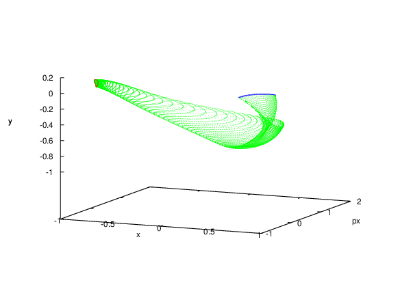
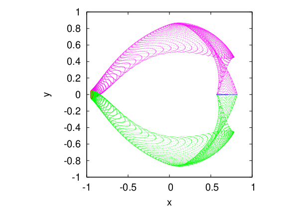
Each Lyapunov orbit is SS-symmetric. It possesses a two dimensional stable manifold and a two dimensional unstable manifold. These manifolds lie on the same energy level as the orbit and their intersection, when restricted to the three dimensional constant energy manifold (4), is transversal. These invariant manifolds are SS-symmetric with respect to each other, meaning that the stable manifold is an image by SS of the unstable manifold (see Figure 3 for the unstable manifold, and Figure 4 for the intersection of manifolds). All these facts are well known and extensively studied numerically.

Our aim in this paper will be firstly to provide a rigorous-computer-assisted proof of existence of the manifold of Lyapunov orbits over a large radius from L2L_{2} (see Figure 2). Secondly, using rigorous-computer-assisted computations, we shall show that for orbits with energies close to the energy of comet Oterma h=1. 515h=1.\,\allowbreak 515 their associated stable and unstable manifolds intersect transversally. Even though such intersections are well known from numerical investigation, to the best of our knowledge this is a first rigorous proof of their existence.
Refer to caption
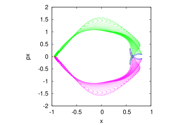
Fig. 3: The Lyapunov orbit in red, its unstable manifold in green, and the intersection of the unstable manifold with section {y=0}\{y=0\} in blue, projected onto x,y,pxx,y,p_{x} coordinates. The figure is for the energy of comet Oterma h=1.515h=1.515 in the Jupiter-Sun system.
Refer to caption
Refer to caption
Fig. 4: The Lyapunov orbit in red, its unstable manifold in green, stable manifold in purple, and their intersections with section {y=0}\{y=0\} in blue, projected onto x,yx,y coordinates (left) and x,pxx,p_{x} coordinates (right). The figure is for the energy of comet Oterma h=1. 515h=1.\,\allowbreak 515 in the Jupiter-Sun system.

2.2 Interval Newton Method

Let XX be a subset of ℝn\mathbb{R}^{n}. We shall denote by [X][X] an interval enclosure of the set XX, that is, a set

[X]=Πi=1n​[ai,bi]⊂ℝn,[X]=\Pi_{i=1}^{n}[a_{i},b_{i}]\subset\mathbb{R}^{n},

such that

X⊂[X].X\subset[X].

Let f:ℝn→ℝnf:\mathbb{R}^{n}\to\mathbb{R}^{n} be a C1C^{1} function and U⊂ℝnU\subset\mathbb{R}^{n}. We shall denote by [D​f​(U)][Df(U)] the interval enclosure of a Jacobian matrix on the set UU. This means that [D​f​(U)][Df(U)] is an interval matrix defined as

[Df(U)]={A∈ℝn×n|Ai​j∈[infx∈Ud​fid​xj(x),supx∈Ud​fid​xj(x)] for all i,j=1,…,n }.[Df(U)]=\left\{A\in\mathbb{R}^{n\times n}|A_{ij}\in\left[\inf_{x\in U}\frac{df_{i}}{dx_{j}}(x),\sup_{x\in U}\frac{df_{i}}{dx_{j}}(x)\right]\text{ for all }i,j=1,\ldots,n\text{ }\right\}.
Theorem 1.

[2] (Interval Newton method) Let f:ℝn→ℝnf:\mathbb{R}^{n}\rightarrow\mathbb{R}^{n} be a C1C^{1} function and X=Πi=1n​[ai,bi]X=\Pi_{i=1}^{n}[a_{i},b_{i}] with ai<bia_{i}<b_{i}. If [D​f​(X)][Df(X)] is invertible and there exists an x0x_{0} in XX such that

N⁡(x0,X):=x0−[D​f​(X)]−1​f​(x0)⊂X,N(x_{0},X):=x_{0}-\left[Df(X)\right]^{-1}f(x_{0})\subset X,

then there exists a unique point x∗∈Xx^{\ast}\in X such that f⁡(x∗)=0.f(x^{\ast})=0.

2.3 Notations

Throughout the paper we shall use a notation ϕ⁡(t,x)\phi(t,x) for the flow, and ΦT​(x)=ϕ⁡(T,x)\Phi_{T}(x)=\phi(T,x) for a time TT shift along trajectory map of (3). For points p=(x,y)p=(x,y) we shall write πx​p\pi_{x}p and πy​p,\pi_{y}p, to denote projections onto coordinates xx and yy respectively. We shall also use the following notation for a cartesian product of sets Πi=1n​Ui=U1×…×Un\Pi_{i=1}^{n}U_{i}=U_{1}\times\ldots\times U_{n}. For A,B⊂ℝnA,B\subset\mathbb{R}^{n} we shall use a notation A+B={a+b|a∈A,b∈B}A+B=\{a+b|a\in A,b\in B\}.

3 Existence of a Family of Lyapunov Orbits

In this section we shall present a method for proving existence of Lyapunov orbits far away from L2L_{2}. The result is in the spirit of the method applied by Wilczak and Zgliczyński in [19, 20] for a Lyapunov orbit with energy h=1. 515h=1.\,515 of the comet Oterma. Our result differs from [19, 20] by the fact that we obtain a smooth family of orbits over a large set, whereas in [19, 20] a single orbit was proved.

We shall consider orbits starting from points of the form (x,0,0,py)(x,0,0,p_{y}) with xx inside an interval

Ix\displaystyle I_{x} =[Ix¯,Ix¯]:=[12​(−1+μ−0.933),−0.933]\displaystyle=[\underline{I_{x}},\overline{I_{x}}]:=\left[\frac{1}{2}(-1+\mu-0.933),-0.933\right] (7)
≈[−0.96602315,−0.933]⊂ℝ.\displaystyle\approx[-0.96602315,-0.933]\subset\mathbb{R}.

Since πx​L2≈−0.93237\pi_{x}L_{2}\approx-0.93237 we see that Ix¯<12​(−1+μ−πx​L2)\underline{I_{x}}<\frac{1}{2}(-1+\mu-\pi_{x}L_{2}), so the interval IxI_{x} stretches from half the distance between the smaller primary and L2L_{2}, almost up to L2L_{2} (see Figure 2, where the orbits are depicted in green, and stretch between an inner and outer orbit depicted in blue).

Let us consider a section Σ={y=0}\Sigma=\{y=0\} and a Poincaré map P:Σ→ΣP:\Sigma\rightarrow\Sigma of (3). We shall interpret the Poincaré map as a function from ℝ3\mathbb{R}^{3} to ℝ3\mathbb{R}^{3} with coordinates x,px,pyx,p_{x},p_{y}. If for a point q=(x,0,py)∈Σq=(x,0,p_{y})\in\Sigma we have πpx​P​(q)=0\pi_{p_{x}}P(q)=0, then by the symmetry property (5) the point qq lies on a periodic orbit (the Poincaré map PP makes a half turn along the orbit starting from qq).

Let us introduce the following notation

f:ℝ2→ℝ,f:\mathbb{R}^{2}\rightarrow\mathbb{R},
f⁡(x,py)=πpx​P​(x,0,py).f(x,p_{y})=\pi_{p_{x}}P(x,0,p_{y}).

To find a periodic orbit for some fixed xx it is sufficient to find a zero of a function

gx​(py):=f⁡(x,py).g_{x}(p_{y}):=f(x,p_{y}).

Let D​P=(d​Pi​j)i,j=1,2,3DP=\left(dP_{i\,j}\right)_{i,j=1,2,3} be the derivative of the map P,P, with indexes 1,2,31,2,3 corresponding to coordinates x,px,pyx,p_{x},p_{y} respectively.

Refer to caption
Fig. 5: The bound for a curve of points q⁡(x)=(x,0,0,κ⁡(x))q(x)=(x,0,0,\kappa(x)) on Lyapunov orbits.
Lemma 2.

Let II and JiJ_{i} for i=0,1i=0,1 be closed intervals such that J0,J1J_{0},J_{1} have the same center point py0p_{y}^{0} and J0⊂J1J_{0}\subset J_{1}. Let x0x^{0} be the center point of II. Let a∈ℝa\in\mathbb{R} and U0,U⊂Σ=ℝ3U_{0},U\subset\Sigma=\mathbb{R}^{3} be sets defined as (see Figure 5)

U0\displaystyle U_{0} ={x0}×{0}×J0,\displaystyle=\{x^{0}\}\times\{0\}\times J_{0},
U\displaystyle U ={(x,0,py)|x∈I,py=a(x−x0)+ι,ι∈J1}.\displaystyle=\left\{(x,0,p_{y})|x\in I,p_{y}=a\left(x-x^{0}\right)+\iota,\iota\in J_{1}\right\}. (8)

If

N:=py0−[πpx​P​(x0,0,py0)d​P​(U0)2 3]⊂J0,N:=p_{y}^{0}-\left[\frac{\pi_{p_{x}}P(x^{0},0,p_{y}^{0})}{dP(U_{0})_{2\,3}}\right]\subset J_{0}, (9)

and

|α−a|<1|I|​(|J1|−|J0|)for all ​α∈[α¯,α¯]:=[−d​P​(U)2 1d​P​(U)2 3],\left|\alpha-a\right|<\frac{1}{|I|}\left(|J_{1}|-|J_{0}|\right)\quad\text{for all }\alpha\in\left[\underline{\alpha},\overline{\alpha}\right]:=\left[-\frac{dP(U)_{2\,1}}{dP(U)_{2\,3}}\right], (10)

then there exists a smooth function κ:I→ℝ\kappa:I\rightarrow\mathbb{R} such that for any x∈Ix\in I a point q⁡(x)=(x,0,0,κ⁡(x))q(x)=(x,0,0,\kappa(x)) lies on an SS-symmetric periodic orbit of (3). Moreover, κ′​(x)∈[α¯,α¯]\kappa^{\prime}(x)\in\left[\underline{\alpha},\overline{\alpha}\right] and q⁡(x)∈Uq(x)\in U for all x∈Ix\in I.

Proof.

Existence of a unique point κ⁡(x0)∈J0\kappa(x_{0})\in J_{0} for which gx0​(κ⁡(x0))=0g_{x_{0}}(\kappa(x_{0}))=0 follows from (9), which implies

py0−[D​gx0​(J0)]−1​gx0​(py0)⊂N⊂J0,p_{y}^{0}-\left[Dg_{x_{0}}(J_{0})\right]^{-1}g_{x_{0}}(p_{y}^{0})\subset N\subset J_{0},

combined with interval Newton method (Theorem 1).

For (10) to hold we need to have 0∉d​P​(U)2 30\notin dP(U)_{2\,3}. For (x,0,py)∈U(x,0,p_{y})\in U we have ∂f∂py​(x,py)∈d​P​(U)2 3\frac{\partial f}{\partial p_{y}}(x,p_{y})\in dP(U)_{2\,3} hence ∂f∂py​(x,py)≠0\frac{\partial f}{\partial p_{y}}(x,p_{y})\neq 0. This means that we can apply the implicit function theorem to obtain a curve κ⁡(x)\kappa(x) for which f⁡(x,κ⁡(x))=0f(x,\kappa(x))=0. We now need to make sure that the curve κ\kappa is defined on the entire interval I.I. At each point xx for which (x,0,κ⁡(x))∈U(x,0,\kappa(x))\in U is defined, by the implicit function theorem we know that

κ′​(x)=−∂f∂x​(x,κ​(x))∂f∂py​(x,κ​(x))∈[−d​P​(U)2 1d​P​(U)2 3].\kappa^{\prime}(x)=-\frac{\frac{\partial f}{\partial x}(x,\kappa(x))}{\frac{\partial f}{\partial p_{y}}(x,\kappa(x))}\in\left[-\frac{dP(U)_{2\,1}}{dP(U)_{2\,3}}\right].

This, by assumption (10), means that we can continue the curve from κ⁡(x0)\kappa(x^{0}) to the whole interval II (see Figure 5). ∎

Refer to caption
Fig. 6: Numerical plot of κ⁡(x)\kappa(x), consisting of 15 00015\,000 points qi0q_{i}^{0} on Lyapunov orbits (in red). The point L2L_{2} is in green. The blue line x=−1+μx=-1+\mu gives an indication of the position of the smaller primary along the xx coordinate.

To apply Lemma 2 we first compute numerically a sequence of points (see Figure 6)

qi0\displaystyle q_{i}^{0} =(xi0,0,0,py,i0)fori=0,…,15 000,\displaystyle=(x_{i}^{0},0,0,p_{y,i}^{0})\quad\text{for}\quad i=0,\ldots,15\,000,
xi0\displaystyle x_{i}^{0} =Ix¯+i15000​(Ix¯−Ix¯),\displaystyle=\underline{I_{x}}+\frac{i}{15000}\left(\overline{I_{x}}-\underline{I_{x}}\right),

where Ix¯\underline{I_{x}}, Ix¯\overline{I_{x}} are defined in (7). The qi0q_{i}^{0} are non-rigorously, numerically computed points on Lyapunov orbits. We then compute (non-rigorously) a sequence of slopes (see Figure 7)

ai∈ℝi=0,…,15 000,a_{i}\in\mathbb{R}\quad i=0,\ldots,15\,000,

define

r=115 000​12​(Ix¯−Ix¯)≈10−6⋅1.1007716,r=\frac{1}{15\,000}\frac{1}{2}(\overline{I_{x}}-\underline{I_{x}})\approx 10^{-6}\cdot 1.1007716,
Ii\displaystyle I_{i} =xi0+[−r,r],\displaystyle=x_{i}^{0}+\left[-r,r\right],
J0,i\displaystyle J_{0,i} =py,i0+10−13⋅[−1,1],\displaystyle=p_{y,i}^{0}+10^{-13}\cdot[-1,1],
J1,i\displaystyle J_{1,i} =py,i0+10−8⋅[−5,5],\displaystyle=p_{y,i}^{0}+10^{-8}\cdot\left[-5,5\right],

and consider sets

U0\displaystyle U_{0} ={xi0}×{0}×J0,i,\displaystyle=\{x_{i}^{0}\}\times\{0\}\times J_{0,i},
Ui\displaystyle U_{i} ={(x,0,py)|x∈Ii,py=ai(x−xi0)+ι,ι∈J1,i}.\displaystyle=\left\{(x,0,p_{y})|x\in I_{i},p_{y}=a_{i}\left(x-x_{i}^{0}\right)+\iota,\iota\in J_{1,i}\right\}.

We apply Lemma 2 repeatedly 15 00015\,000 times, and obtain the following theorem.

Refer to caption
Fig. 7: Numerical plot of κ′​(x)\kappa^{\prime}(x), consisting of 15 00015\,000 points aia_{i}
Theorem 3 (First main result).

Let IxI_{x} be the interval from (7). Then there exists a curve q⁡(x)=(x,0,0,κ⁡(x))q(x)=(x,0,0,\kappa(x)) of points on Lyapunov orbits with κ:Ix→ℝ\kappa:I_{x}\rightarrow\mathbb{R}, which lies within a 5⋅10−85\cdot 10^{-8} distance from the piecewise linear curve joining the 15 00015\,000 points qi0q^{0}_{i} on Figure 6.

The proof of Theorem 3 took 55 hours and 4343 minutes on a standard laptop.

Remark 4.

Using above described method it is impossible to continue with the orbits to L2L_{2}. At the fixed point one would need to apply alternative methods, such as the method of majorants [18], Lyapunov theorem by tracing the radius of convergence of the normal form [17], or topological-computer-assisted tools such as [5, 7].

4 Outline of Results for Intersections of Invariant Manifolds

In the reminder of the paper we shall focus our attention on orbits starting from q⁡(x)=(x,0,0,κ⁡(x))q(x)=(x,0,0,\kappa(x)) with x∈Ix\in I for

I\displaystyle I =[I¯,I¯]:=x0+[−1,1]⋅10−9,\displaystyle=[\underline{I},\overline{I}]:=x^{0}+[-1,1]\cdot 10^{-9}, (11)
x0\displaystyle x^{0} =−0.9510055339445208.\displaystyle=-0.9510055339445208.

Such orbits have energy close to the energy of the comet Oterma h=1.515h=1.515.

Let us introduce a notation Λ\Lambda for a family of Lyapunov orbits, which start from q⁡(x)q(x) with x∈Ix\in I

Λ={ϕ(t,q(x))|t∈ℝ,q(x)=(x,0,0,κ(x)),x∈I}.\Lambda=\{\phi(t,q(x))|t\in\mathbb{R},q(x)=(x,0,0,\kappa(x)),x\in I\}. (12)

For x∈I,x\in I, let L⁡(x)⊂ΛL(x)\subset\Lambda denote the Lyapunov orbit which starts from q⁡(x).q(x).

Throughout the reminder of the paper we shall prove the following theorem.

Theorem 5 (Second main result).

Λ\Lambda is a normally hyperbolic invariant manifold with a boundary. Each orbit L⁡(x)⊂ΛL(x)\subset\Lambda possesses a two dimensional stable manifold Ws​(L​(x))W^{s}(L(x)) and a two dimensional unstable manifold Wu​(L​(x)).W^{u}(L(x)). The manifolds Ws​(L​(x))W^{s}(L(x)) and Wu​(L​(x))W^{u}(L(x)) intersect and the intersection, when restricted to the constant energy manifold M⁡(H⁡(L⁡(x)))M(H(L(x))), is transversal (see (4) for definition of MM).

Numerical plots of the intersection of manifolds that we shall prove are given in Figure 4.

Theorem 5 will be proved with computer assistance. During the proof we shall obtain rigorous bounds on the region and the angle at which the manifolds intersect (see Figure 14).

The size of interval II (11) is very small. When translated the real life distance in the Jupiter-Sun system, its length is just slightly over one and a half kilometer. This is practically a single point. We need to start with such a small set to obtain our result. Thanks to this we obtain sharp estimates on the intersection of Ws​(L​(x))W^{s}(L(x)), Wu​(L​(x))W^{u}(L(x)). To consider a larger set of Lyapunov orbits one would need to iterate the procedure a number of times. This can be done without any difficulty apart from necessary time for computation. The proof of Theorem 5 took 4646 minutes on a standard laptop. Using clusters one could cover a larger interval II in reasonable time.

5 Hyperbolicity of Lyapunov Orbits and Foliation by Energy

In this section we shall show that each orbit L⁡(x)⊂ΛL(x)\subset\Lambda lies on a different energy level. We shall also show that each orbit L⁡(x)L(x) (when considered on its constant energy manifold) is hyperbolic. In other words, we shall show that Λ\Lambda is a normally hyperbolic manifold with a boundary.

We start with a simple remark.

Remark 6.

If for all x∈Ix\in I we have dd​x​H​(q⁡(x))≠0,\frac{d}{dx}H(q(x))\neq 0, then Lyapunov orbits with different xx have different energies. Note that the set UU and the bound on the derivative of κ′​(x)\kappa^{\prime}(x) from Lemma 2 can be used to obtain

dd​x​H​(q⁡(x))∈[∂H∂x​(U)+∂H∂py​(U)​κ′​(U)].\frac{d}{dx}H(q(x))\in\left[\frac{\partial H}{\partial x}(U)+\frac{\partial H}{\partial p_{y}}(U)\kappa^{\prime}(U)\right].

We shall now give a simple lemma which can be used to show that our Lyapunov orbits are hyperbolic.

In what follows in this section, let P:Σ→ΣP:\Sigma\rightarrow\Sigma be a second return Poincaré map for Σ={y=0}.\Sigma=\{y=0\}. This means that each point q⁡(x)=(x,0,0,κ⁡(x)),q(x)=(x,0,0,\kappa(x)), with x∈Ix\in I, is a fixed point of P.P. We shall interpret the Poincaré map as a function from ℝ3\mathbb{R}^{3} to ℝ3\mathbb{R}^{3} with coordinates x,px,pyx,p_{x},p_{y}.

Lemma 7.

Let UU be the set given by (8) in Lemma 2. Assume that for any 1×21\times 2 matrix AA

A∈[(−(∂H∂x)−1​(∂H∂px∂H∂py))​(U)]A\in\left[\left(-\left(\frac{\partial H}{\partial x}\right)^{-1}\left(\begin{array}[c]{cc}\frac{\partial H}{\partial p_{x}}&\frac{\partial H}{\partial p_{y}}\end{array}\right)\right)(U)\right] (13)

and any 2×22\times 2 matrix BB

B∈[((d​P2 1d​P3 1)​A+(d​P2 2d​P2 3d​P3 2d​P3 3))​(U)]B\in\left[\left(\left(\begin{array}[c]{c}dP_{2\,1}\\ dP_{3\,1}\end{array}\right)A+\left(\begin{array}[c]{cc}dP_{2\,2}&dP_{2\,3}\\ dP_{3\,2}&dP_{3\,3}\end{array}\right)\right)\left(U\right)\right] (14)

the spectrum of BB consists of two real eigenvalues λ1,λ2\lambda_{1},\lambda_{2} satisfying |λ1|>1>|λ2|.\left|\lambda_{1}\right|>1>\left|\lambda_{2}\right|. Then for any x∈Ix\in I the Lyapunov orbit starting from q⁡(x),q(x), restricted to the constant energy manifold M⁡(H⁡(q⁡(x)))M(H(q(x))), is a hyperbolic orbit.

Proof.

Let us fix some x^∈I.\hat{x}\in I. For our assumptions to hold, AA from (13) needs to be properly defined. This means that ∂H∂x​(q​(x^))≠0\frac{\partial H}{\partial x}(q(\hat{x}))\neq 0. By the implicit function theorem there exists a function x⁡(px,py)x(p_{x},p_{y}) with x⁡(0,κ⁡(x^))=x^x(0,\kappa(\hat{x}))=\hat{x} such that H⁡(x⁡(px,py),0,px,py)=H⁡(q⁡(x^))H(x(p_{x},p_{y}),0,p_{x},p_{y})=H(q(\hat{x})) and

(∂x∂px∂x∂py)​(0,κ⁡(x^))=−(1∂H∂x​(∂H∂px∂H∂py))​(0,κ⁡(x^)).\left(\begin{array}[c]{cc}\frac{\partial x}{\partial p_{x}}&\frac{\partial x}{\partial p_{y}}\end{array}\right)\left(0,\kappa(\hat{x})\right)=-\left(\frac{1}{\frac{\partial H}{\partial x}}\left(\begin{array}[c]{cc}\frac{\partial H}{\partial p_{x}}&\frac{\partial H}{\partial p_{y}}\end{array}\right)\right)\left(0,\kappa(\hat{x})\right). (15)

The Lyapunov orbit starting from q⁡(x^)q(\hat{x}) is contained in the constant energy manifold M⁡(H⁡(q⁡(x^)))M(H(q(\hat{x}))). Let us consider V=M(H(q(x^)))∩{y=0}V=M(H(q(\hat{x})))\cap\{y=0\} and a Poincaré map P~:V→V\tilde{P}:V\rightarrow V. In a neighborhood of q⁡(x^)q(\hat{x}) the manifold VV can be parameterized by (px,py).\left(p_{x},p_{y}\right). Since

P~​(px,py)=π(px,py)​P​(x⁡(px,py),px,py)\tilde{P}(p_{x},p_{y})=\pi_{(p_{x},p_{y})}P(x(p_{x},p_{y}),p_{x},p_{y})

we have

D​P~​(0,κ⁡(x^))\displaystyle D\tilde{P}\left(0,\kappa(\hat{x})\right) (16)
=((π(px,py)​∂P∂x)​(∂x∂px∂x∂py)+(d​P2 2d​P2 3d​P3 2d​P3 3))​(x^,0,κ⁡(x^)).\displaystyle=\left(\left(\pi_{(p_{x},p_{y})}\frac{\partial P}{\partial x}\right)\left(\begin{array}[c]{cc}\frac{\partial x}{\partial p_{x}}&\frac{\partial x}{\partial p_{y}}\end{array}\right)+\left(\begin{array}[c]{cc}dP_{2\,2}&dP_{2\,3}\\ dP_{3\,2}&dP_{3\,3}\end{array}\right)\right)\left(\hat{x},0,\kappa(\hat{x})\right).

By (15), (16) and our assumption about the spectrum of BB of from (14), follows that (0,κ⁡(x^))\left(0,\kappa(\hat{x})\right) is a hyperbolic fixed point for the map P~.\tilde{P}. This means that the Lyapunov orbit starting from q⁡(x^)q(\hat{x}), restricted to the constant energy manifold M⁡(H⁡(q⁡(x^)))M(H(q(\hat{x}))) is hyperbolic. ∎

Remark 8.

Since BB from (14) is a 2×22\times 2 matrix, estimation of its eigenvalues is straightforward. Here we profit from the the reduction of dimension made by restricting to a constant energy manifold.

Since we consider a small part of the family of orbits (11), we can obtain a much tighter enclosure of the curve κ⁡(x)\kappa(x) for x∈Ix\in I than from Theorem 3. Let

py0=−0.836804179646973J0=py0+[−1,1]⋅10−13a=−4.506866203376769J1=py0+[−1,1]⋅10−12\begin{array}[c]{lll}p_{y}^{0}=&-0.836804179646973&J_{0}=p_{y}^{0}+[-1,1]\cdot 10^{-13}\\ a=&-4.506866203376769&J_{1}=p_{y}^{0}+[-1,1]\cdot 10^{-12}\end{array} (20)

and

U={(x,0,0,py)|x∈I,py=a(x−x0)+ι,ι∈J1}.U=\left\{(x,0,0,p_{y})|x\in I,p_{y}=a\left(x-x^{0}\right)+\iota,\iota\in J_{1}\right\}. (21)
Proposition 9.

For x∈Ix\in I, with II from (11), we have q⁡(x)=(x,0,0,κ⁡(x))⊂Uq(x)=(x,0,0,\kappa(x))\subset U and

κ′​(x)\displaystyle\kappa^{\prime}(x) ∈[−4.506980818,−4.506751634],\displaystyle\in[-4.506980818,-4.506751634], (22)
dd​x​H​(q⁡(x))\displaystyle\frac{d}{dx}H(q(x)) ∈[−0.3670937615,−0.3670674516],\displaystyle\in[-0.3670937615,-0.3670674516], (23)
H⁡(I¯,0,0,a⁡(I¯−x0)+J1)\displaystyle H(\underline{I},0,0,a(\underline{I}-x_{0})+J_{1}) ∈[−1.514999999635,−1.514999999631],\displaystyle\in[-1.514999999635,-1.514999999631],
H⁡(I¯,0,0,a⁡(I¯−x0)+J1)\displaystyle H(\overline{I},0,0,a(\overline{I}-x_{0})+J_{1}) ∈[−1.515000000369,−1.515000000365].\displaystyle\in[-1.515000000369,-1.515000000365].

Moreover, the orbits (when considered on their constant energy manifolds) are hyperbolic, and we have following bounds for the eigenvalues

λ1\displaystyle\lambda_{1} ∈[1450.24,1481.68],\displaystyle\in\left[1450.24,1481.68\right], (24)
λ2\displaystyle\lambda_{2} ∈10−4​[6.74909,6.89541].\displaystyle\in 10^{-4}\left[6.74909,6.89541\right].
Proof.

The proof was performed with computer assistance. It required no subdivision of UU and the computation took less than two seconds on a standard laptop.

Existence of q⁡(x)⊂Uq(x)\subset U was shown using Lemma 2. From it also follows the bound (22) for κ′​(x).\kappa^{\prime}(x). The bound (23) follows from Remark 6. Hyperbolicity and bounds (24) follow from Lemma 7. ∎

6 Cone Conditions and Bounds for Unstable Manifolds of Saddle-Center Fixed Points

In this section we provide a topological tool that can be used for rigorous-computer-assisted detection of unstable manifolds of saddle-center fixed points. The method is a modification of [21], where instead of saddle-center a standard hyperbolic fixed point was considered. The content of this section is a general result. In section 7 we return to the PRC3BP and show how to apply it for the proof of Theorem 5.

Let F:ℝn→ℝnF:\mathbb{R}^{n}\rightarrow\mathbb{R}^{n} be a CkC^{k} diffeomorphism with a fixed point v∗∈ℝnv^{\ast}\in\mathbb{R}^{n} and k≥1.k\geq 1. Assume that for eigenvalues λ1,λ2,…,λn\lambda_{1},\lambda_{2},\ldots,\lambda_{n} from the spectrum of D​F​(v∗)DF(v^{\ast}) we have

|re​λ1|\displaystyle\left|\text{re}\lambda_{1}\right| >m>1,\displaystyle>m>1, (25)
|re​λi|\displaystyle\left|\text{re}\lambda_{i}\right| <mfor i=2,…,n.\displaystyle<m\quad\text{for }i=2,\ldots,n.

Let Wu​(v∗)W^{u}(v^{\ast}) denote the unstable manifold of v∗v^{\ast} associated with the eigenvalue λ1\lambda_{1}

Wu(v∗)={v|‖F−n(v)−v∗‖<Cm−n for all n∈ℕ and some C>0}.W^{u}\left(v^{\ast}\right)=\left\{v|\left\|F^{-n}(v)-v^{\ast}\right\|<Cm^{-n}\text{ for all }n\in\mathbb{N}\text{ and some }C>0\right\}.

Let u=1u=1 and c=n−1c=n-1. The notations uu and cc will stand for ”unstable” and ”central” coordinates of FF at v∗v^{\ast}. Consider two balls BuB_{u} and Bc,B_{c}, of dimensions uu and cc respectively, such that Bu×BcB_{u}\times B_{c} is centered at v∗v^{\ast}. For a point v∈ℝu×ℝcv\mathbf{\in}\mathbb{R}^{u}\times\mathbb{R}^{c} we shall write v=(𝗑,𝗒),v=\left(\mathsf{x},\mathsf{y}\right), with 𝗑∈ℝu,\mathsf{x}\in\mathbb{R}^{u}, 𝗒∈ℝc.\mathsf{y}\mathbf{\in}\mathbb{R}^{c}. In these notations we shall also write the fixed point as v∗=(𝗑∗,𝗒∗).v^{\ast}=\left(\mathsf{x}^{\ast},\mathsf{y}^{\ast}\right).

Remark 10.

We do not need to assume that (𝗑,0)(\mathsf{x},0) is the eigenvector associated with λ1\lambda_{1} and that vectors (0,𝗒)(0,\mathsf{y}) span the eigenspace of λ2,…,λn\lambda_{2},\ldots,\lambda_{n}. For our method to work it is enough if these vectors are ”roughly” aligned with the eigenspaces. This is important for us, since in any computer assisted computation it is usually not possible to compute the eigenvectors with full precision.

Let α∈ℝ,\alpha\in\mathbb{R,} α>0\alpha>0 and consider a function Q:ℝu×ℝc→ℝQ:\mathbb{R}^{u}\times\mathbb{R}^{c}\rightarrow\mathbb{R}

Q⁡(𝗑,𝗒)=α​𝗑2−‖𝗒‖2.Q(\mathsf{x},\mathsf{y})=\alpha\mathsf{x}^{2}-\left\|\mathsf{y}\right\|^{2}.

For v0∈ℝu×ℝcv_{0}\in\mathbb{R}^{u}\times\mathbb{R}^{c} we shall use a notation Q+​(v0)Q^{+}(v_{0}) for a cone

Q+​(v0)={v|Q⁡(v−v0)≥0}.Q^{+}(v_{0})=\left\{v|Q(v-v_{0})\geq 0\right\}.

Let us assume that α\alpha is chosen sufficiently small so that Q+​(v∗)∩Bu×BcQ^{+}(v^{\ast})\cap B_{u}\times B_{c} does not intersect with Bu×∂BcB_{u}\times\partial B_{c} (See Figure 8).

Definition 11.

We shall say that h:Bu→Bu×Bch:B_{u}\rightarrow B_{u}\times B_{c} is a horizontal disc in Bu×BcB_{u}\times B_{c} for cones given by QQ if h⁡(𝗑∗)=v∗,h(\mathsf{x}^{\ast})=v^{\ast}, π𝗑​h​(𝗑)=𝗑\pi_{\mathsf{x}}h(\mathsf{x})=\mathsf{x} and for any 𝗑1≠𝗑2\mathsf{x}_{1}\neq\mathsf{x}_{2} holds Q⁡(h⁡(𝗑1)−h⁡(𝗑2))>0.Q\left(h(\mathsf{x}_{1})-h(\mathsf{x}_{2})\right)>0.

Refer to caption
Fig. 8: Construction of the curve (𝗑,wu​(𝗑))(\mathsf{x},w^{u}(\mathsf{x})) which lies on the unstable manifold of v∗v^{\ast}.
Lemma 12.

Assume that for any v1,v2∈Q+​(v∗),v_{1},v_{2}\in Q^{+}(v^{\ast}), such that Q⁡(v1−v2)≥0,Q(v_{1}-v_{2})\geq 0, we have

Q⁡(F⁡(v1)−F⁡(v2))>0.Q(F(v_{1})-F(v_{2}))>0. (26)

Let mm be the constant from (25). If for any v∈B,v\in B, v≠v∗,v\neq v^{\ast}, Q⁡(v−v∗)≥0Q(v-v^{\ast})\geq 0 holds

‖F⁡(v)−v∗‖>m⁡‖v−v∗‖,\left\|F(v)-v^{\ast}\right\|>m\left\|v-v^{\ast}\right\|, (27)

then Wu​(v∗)⊂Q+​(v∗).W^{u}\left(v^{\ast}\right)\subset Q^{+}(v^{\ast}). Moreover, there exists a function wu:Bu→Bcw^{u}:B_{u}\rightarrow B_{c} such that (i​d,wu)​(Bu)=Wu​(v∗)∩U,(id,w^{u})(B_{u})=W^{u}(v^{\ast})\cap U, and for any 𝗑1,𝗑2∈Bu,\mathsf{x}_{1},\mathsf{x}_{2}\in B_{u}, 𝗑1≠𝗑2\mathsf{x}_{1}\neq\mathsf{x}_{2}

Q⁡((𝗑1,wu​(𝗑1))−(𝗑2,wu​(𝗑2)))>0Q((\mathsf{x}_{1},w^{u}\left(\mathsf{x}_{1}\right))-(\mathsf{x}_{2},w^{u}\left(\mathsf{x}_{2}\right)))>0 (28)

and

‖(wu)′​(𝗑)‖≤αfor all ​𝗑∈Bu.\left\|\left(w^{u}\right)^{\prime}\left(\mathsf{x}\right)\right\|\leq\sqrt{\alpha}\quad\text{for all }\mathsf{x}\in B_{u}. (29)
Proof.

We shall first show that for any 𝗑0∈Bu\{𝗑∗}\mathsf{x}_{0}\in B_{u}\backslash\{\mathsf{x}^{\ast}\} there exists a point v0=(𝗑0,wu​(𝗑0))∈Q+​(v∗)v_{0}=(\mathsf{x}_{0},w^{u}(\mathsf{x}_{0}))\in Q^{+}(v^{\ast}) such that v0∈Wu​(v∗).v_{0}\in W^{u}(v^{\ast}). Let h0​(𝗑)=(𝗑,𝗒∗)h_{0}(\mathsf{x})=(\mathsf{x},\mathsf{y}^{\ast}) be a horizontal disc (See Figure 8). Observe that F⁡(h0​(𝗑∗))=F⁡(𝗑∗,𝗒∗)=v∗F(h_{0}(\mathsf{x}^{\ast}))=F(\mathsf{x}^{\ast},\mathsf{y}^{\ast})=v^{\ast}. By assumptions (26), (27) the curve F​(h0​(𝗑))F(h_{0}(\mathsf{x})) is contained in Q+​(v∗)Q^{+}(v^{\ast}) and F⁡(h0​(∂Bu))∩Bu×Bc=∅F(h_{0}(\partial B_{u}))\cap B_{u}\times B_{c}=\emptyset. Moreover, by assumption (26) for any 𝗑1,𝗑2∈Bu,\mathsf{x}_{1},\mathsf{x}_{2}\in B_{u}, 𝗑1≠𝗑2\mathsf{x}_{1}\neq\mathsf{x}_{2}

Q⁡(F⁡(h0​(𝗑1))−F⁡(h0​(𝗑2)))>Q⁡(h0​(𝗑1)−h0​(𝗑2))>0,Q(F(h_{0}(\mathsf{x}_{1}))-F(h_{0}(\mathsf{x}_{2})))>Q(h_{0}(\mathsf{x}_{1})-h_{0}(\mathsf{x}_{2}))>0,

which means that {F⁡(h0​(𝗑))|𝗑∈Bu}∩Bu×Bc\{F(h_{0}(\mathsf{x}))|\mathsf{x}\in B_{u}\}\cap B_{u}\times B_{c} is a graph of a horizontal disc. Let us denote this disc by h1h_{1} and observe that h1​(𝗑∗)=v∗.h_{1}(\mathsf{x}^{\ast})=v^{\ast}. In other words, let h1h_{1} be the graph transform of the disc h0.h_{0}.

Taking F​(h1​(𝗑))F(h_{1}(\mathsf{x})) and applying an identical argument, we observe that

{F⁡(h1​(𝗑))|𝗑∈Bu}∩Bu×Bc\{F(h_{1}(\mathsf{x}))|\mathsf{x}\in B_{u}\}\cap B_{u}\times B_{c}

is a graph of a horizontal disc h2.h_{2}. Repeating this procedure we can construct a sequence of horizontal discs h0,h1,h2,…h_{0},h_{1},h_{2},\ldots. For a fixed 𝗑0\mathsf{x}_{0}, due to compactness of closure of Bc,B_{c}, there exists a subsequence hki​(𝗑0)h_{k_{i}}(\mathsf{x}_{0}) convergent to some point v0∈Bu×cl​Bcv_{0}\in B_{u}\times\mathrm{cl}B_{c}. For any i,n∈ℕi,n\in\mathbb{N} with ki>nk_{i}>n the point F−n​(hki​(𝗑0))F^{-n}(h_{k_{i}}(\mathsf{x}_{0})) lies on the graph of hki−nh_{k_{i}-n} and hence is also in Q+​(v∗).Q^{+}(v^{\ast}). This means that for any n∈ℕn\in\mathbb{N}

F−n​(v0)=limi→∞F−n​(hki​(𝗑0))∈Q+​(v∗).F^{-n}(v_{0})=\lim_{i\rightarrow\infty}F^{-n}(h_{k_{i}}(\mathsf{x}_{0}))\in Q^{+}(v^{\ast}).

By assumption (27) we have

‖F−n​(v0)−v∗‖<1mn​‖v0−v∗‖,\left\|F^{-n}(v_{0})-v^{\ast}\right\|<\frac{1}{m^{n}}\left\|v_{0}-v^{\ast}\right\|,

which means that v0∈Wu​(v∗)v_{0}\in W^{u}\left(v^{\ast}\right). By construction π𝗑​v0=𝗑0\pi_{\mathsf{x}}v_{0}=\mathsf{x}_{0}, hence we can define wu​(𝗑0):=π𝗒​v0w^{u}(\mathsf{x}_{0}):=\pi_{\mathsf{y}}v_{0}.

By the stable/unstable manifold theorem, there exists a small interval Iε=(𝗑∗−ε,𝗑∗+ε)I_{\varepsilon}=(\mathsf{x}^{\ast}-\varepsilon,\mathsf{x}^{\ast}+\varepsilon) in which {(𝗑,wu​(𝗑))|𝗑∈Iε}\{(\mathsf{x},w^{u}(\mathsf{x}))|\mathsf{x}\in I_{\varepsilon}\} is a CkC^{k} curve which gives full description of Wu​(v∗).W^{u}\left(v^{\ast}\right). Since (𝗑,wu​(𝗑))⊂Q+​(v∗)(\mathsf{x},w^{u}(\mathsf{x}))\subset Q^{+}(v^{\ast}) we have (1,(wu)′​(𝗑∗))∈Q+​(0).(1,(w^{u})^{\prime}(\mathsf{x}^{\ast}))\in Q^{+}(0). Since for sufficiently small ε\varepsilon the vector (1,(wu)′​(𝗑))(1,\left(w^{u}\right)^{\prime}(\mathsf{x})) is arbitrarily close to (1,(wu)′​(𝗑∗)),(1,(w^{u})^{\prime}(\mathsf{x}^{\ast})), for 𝗑1,𝗑2∈Iε\mathsf{x}_{1},\mathsf{x}_{2}\in I_{\varepsilon}

Q⁡((𝗑1,wu​(𝗑1))−(𝗑2,wu​(𝗑2)))>0.Q\left((\mathsf{x}_{1},w^{u}(\mathsf{x}_{1}))-(\mathsf{x}_{2},w^{u}(\mathsf{x}_{2}))\right)>0. (30)

Iterating the curve (𝗑,wu​(𝗑))(\mathsf{x},w^{u}(\mathsf{x})) through FF, by (26), (27) we obtain our function wu:Bu→Bcw^{u}:B_{u}\rightarrow B_{c}. Note that by our construction for any 𝗑1,𝗑2∈Bu\mathsf{x}_{1},\mathsf{x}_{2}\in B_{u} inequality (30) holds. This implies that for any 𝗑1,𝗑2∈Bu\mathsf{x}_{1},\mathsf{x}_{2}\in B_{u}

‖wu​(𝗑1)−wu​(𝗑2)‖2|𝗑1−𝗑2|2<α,\frac{\left\|w^{u}(\mathsf{x}_{1})-w^{u}(\mathsf{x}_{2})\right\|^{2}}{\left|\mathsf{x}_{1}-\mathsf{x}_{2}\right|^{2}}<\alpha,

which in turn gives (29). ∎

Remark 13.

Lemma 12 can easily be generalized to higher dimension of Wu​(v∗)W^{u}(v^{\ast}). The proof would be identical, taking Q⁡(𝗑,𝗒)=α​‖𝗑‖2−‖𝗒‖2Q(\mathsf{x},\mathsf{y})=\alpha\|\mathsf{x}\|^{2}-\|\mathsf{y}\|^{2}. Here we have set up our discussion so that Wu​(v∗)W^{u}(v^{\ast}) is one dimensional simply because this is what we shall need for our application to the PRC3BP.

Remark 14.

By taking the inverse map, Lemma 12 can be used to prove existence of stable manifolds.

To verify assumptions (26) and (27) in practice, it is best to make use of an interval matrix 𝐀=[D​F​(Q+​(v∗))].\mathbf{A}=[DF(Q^{+}(v^{\ast}))]. Then for any v1,v2∈Q+​(v∗)v_{1},v_{2}\in Q^{+}(v^{\ast}) we have

F⁡(v1)−F⁡(v2)=∫01D​F​(v2+t⁡(v1−v2))​𝑑t⋅(v1−v2)∈𝐀⁡(v1−v2).F(v_{1})-F(v_{2})=\int_{0}^{1}DF\left(v_{2}+t\left(v_{1}-v_{2}\right)\right)dt\cdot\left(v_{1}-v_{2}\right)\in\mathbf{A}\left(v_{1}-v_{2}\right). (31)

This means that

F⁡(v)−v∗⊂𝐀⁡(v−v∗).F(v)-v^{\ast}\subset\mathbf{A}\left(v-v^{\ast}\right). (32)

To verify (27) using (32) we can apply Lemma 29 from the Appendix.

Let us now turn to verification of (26). Let CQC_{Q} be a diagonal matrix such that vT​CQ​v=Q⁡(v).v^{T}C_{Q}v=Q(v). Equation (31) gives an estimate

Q⁡(F⁡(v1)−F⁡(v2))⊂(v1−v2)T​𝐀T​CQ​𝐀​(v1−v2).Q\left(F(v_{1})-F(v_{2})\right)\subset\left(v_{1}-v_{2}\right)^{T}\mathbf{A}^{T}C_{Q}\mathbf{A}\left(v_{1}-v_{2}\right). (33)

To verify (26) using (33) we can apply Lemma 30 from the Appendix.

7 Rigorous Bounds for Invariant Manifolds associated with Lyapunov Orbits

In this section we give a proof of Theorem 5. In sections 7.1 and 7.2 we shall show how to apply the method from section 6 to detect fibers of unstable manifolds of Lyapunov orbits. In section 7.3 we shall show how to prove that the manifolds intersect. Using these results, in section 7.4 we give a computer assisted proof Theorem 5.

7.1 Parameterization Method

The method from section 6 requires a good change of coordinates which ”straightens out” the unstable manifold. We shall obtain such a change of coordinates using a parameterization method. In this subsection we give an outline of this procedure.

In this section we shall fix some x∈Ix\in I and show how to find an unstable fiber of a point

q0=q⁡(x)=(x,0,0,κ⁡(x))∈L⁡(x).q_{0}=q(x)=\left(x,0,0,\kappa(x)\right)\in L(x).

We shall use a notation τ=τ⁡(q0)\tau=\tau(q_{0}) for the return time along the trajectory. The point q0q_{0} is a saddle center fixed point for a τ\tau-time map Φτ:ℝ4→ℝ4.\Phi_{\tau}:\mathbb{R}^{4}\rightarrow\mathbb{R}^{4}.

Let CC denote a matrix which brings D​Φτ​(q0)D\Phi_{\tau}\left(q_{0}\right) to real Jordan form. By Φ~τ:ℝ4→ℝ4\tilde{\Phi}_{\tau}:\mathbb{R}^{4}\rightarrow\mathbb{R}^{4} we shall denote the time τ\tau map in the linearized local coordinates

Φ~τ​(v):=C−1​(Φτ​(q0+C​v)−q0).\tilde{\Phi}_{\tau}\left(v\right):=C^{-1}\left(\Phi_{\tau}\left(q_{0}+Cv\right)-q_{0}\right).

Let Wu​(Φ~τ,0)W^{u}(\tilde{\Phi}_{\tau},0) denote the unstable manifold of Φ~τ\tilde{\Phi}_{\tau} at zero. If we can find a function

K=(K0,K1,K2,K3):ℝ→ℝ4,K=\left(K_{0},K_{1},K_{2},K_{3}\right):\mathbb{R\rightarrow R}^{4},

which for all 𝗑\mathsf{x} in an interval I0=[𝗑¯,𝗑¯],I_{0}=[\underline{\mathsf{x}},\overline{\mathsf{x}}], 𝗑¯<0<𝗑¯,\underline{\mathsf{x}}<0<\overline{\mathsf{x}}, is a solution of a cohomology equation

Φ~τ​(K⁡(𝗑))=K⁡(λ​𝗑),\tilde{\Phi}_{\tau}\left(K(\mathsf{x})\right)=K(\lambda\mathsf{x}), (34)

then K⁡(𝗑)⊂Wu​(Φ~τ,0)K(\mathsf{x})\subset W^{u}(\tilde{\Phi}_{\tau},0) for 𝗑∈I0.\mathsf{x}\in I_{0}.

Once KK is established we can consider a nonlinear change of coordinates

ψ=(ψ0,ψ1,ψ2,ψ3):ℝ4→ℝ4\psi=\left(\psi_{0},\psi_{1},\psi_{2},\psi_{3}\right):\mathbb{R}^{4}\rightarrow\mathbb{R}^{4}

defined as

ψ0​(𝗑,𝗒1,𝗒2,𝗒3)\displaystyle\psi_{0}\left(\mathsf{x},\mathsf{y}_{1},\mathsf{y}_{2},\mathsf{y}_{3}\right) =K0​(𝗑)−(𝗒1​K1′​(𝗑)+𝗒2​K2′​(𝗑)+𝗒3​K3′​(𝗑)),\displaystyle=K_{0}(\mathsf{x})-\left(\mathsf{y}_{1}K_{1}^{\prime}(\mathsf{x})+\mathsf{y}_{2}K_{2}^{\prime}(\mathsf{x})+\mathsf{y}_{3}K_{3}^{\prime}(\mathsf{x})\right), (35)
ψi​(𝗑,𝗒1,𝗒2,𝗒3)\displaystyle\psi_{i}\left(\mathsf{x},\mathsf{y}_{1},\mathsf{y}_{2},\mathsf{y}_{3}\right) =Ki(𝗑)+𝗒iK0′(𝗑)for i=1,2,3.\displaystyle=K_{i}(\mathsf{x})+\mathsf{y}_{i}K_{0}^{\prime}(\mathsf{x})\quad\text{for }i=1,2,3.

Note that ψ⁡(𝗑,0)=K⁡(𝗑)\psi(\mathsf{x},0)=K(\mathsf{x}) gives points on the unstable manifold of the fixed point for the map Φ~τ.\tilde{\Phi}_{\tau}. The intuitive idea behind (35) is to orthogonalize coordinates around K⁡(𝗑)K(\mathsf{x}) (see Figure 9).

Let us define a local map

F=ψ−1∘Φ~τ∘ψ.F=\psi^{-1}\circ\tilde{\Phi}_{\tau}\circ\psi.

Such map will play the role of FF from section 6. Observe that

{C​ψ​(K⁡(𝗑))+q0|𝗑∈I0}⊂C​ψ​(Wu​(F,0))+q0=Wu​(Φτ,q0)⊂Wu​(L⁡(x0)).\{C\psi\left(K(\mathsf{x})\right)+q_{0}|\mathsf{x}\in I_{0}\}\subset C\psi\left(W^{u}\left(F,0\right)\right)+q_{0}=W^{u}\left(\Phi_{\tau},q_{0}\right)\subset W^{u}(L(x_{0})).
Refer to caption
Fig. 9: The nonlinear change of coordinates ψ.\psi.

7.2 Bounds for Unstable Fibers through Parameterization and Cone conditions

The map ψ\psi (35) gives us a change of coordinates which locally ”straightens out” the unstable manifold. The problem with applying the procedure from section 7.1 in practice lies in the fact that usually finding an analytic formula for KK satisfying (34) is impossible. The best that can be done is to find a KK which is a polynomial approximation of a solution of (34). This can be done by expanding Φ~τ\tilde{\Phi}_{\tau} into a Taylor series and inductively comparing the coefficients in (34) (for a detailed description of this method we refer the reader to [4]; see in particular Section 4 and Theorem 4.1). If we find such an approximate solution of (34), then the set {(𝗑,0)|𝗑∈I0}\{(\mathsf{x},0)|\mathsf{x}\in I_{0}\} is no longer the unstable manifold for FF (defined by (36)), but its approximation. Even though then our description of the unstable fiber is not entirely accurate, we can apply the method from Section 6 to obtain a rigorous enclosure of Wu​(F,0)W^{u}\left(F,0\right). This enclosure can then be transported to the original coordinates.

In this Section we shall assume that q0q_{0} is an arbitrary point close to q⁡(x)=(x,0,0,κ⁡(x))q(x)=(x,0,0,\kappa(x)) for x∈I,x\in I, CC is some given matrix and K:ℝ→ℝ4K:\mathbb{R\rightarrow R}^{4} is some given polynomial and that ψ\psi is defined by (35).

Remark 15.

Let us stress that the point q0q_{0} is a numerical approximation of q⁡(x),q(x), the matrix CC will be a (non-rigorous) numerically obtained estimate for the change into Jordan form of the map Φτ\Phi_{\tau}. We do not assume that this change is rigorously computed. This is practically impossible due to the fact that we do not have an analytic formula for D​Φτ​(q0)D\Phi_{\tau}\left(q_{0}\right). For us the matrix CC is simply some approximation of the matrix which takes D​Φτ​(q0)D\Phi_{\tau}\left(q_{0}\right) into Jordan form. Let us note that it is not difficult to find an interval matrix 𝐂−1\mathbf{C}^{-1} such that the inverse matrix of our CC is contained in 𝐂−1\mathbf{C}^{-1}.

Remark 16.

In our setting the polynomial KK is an approximation of the solution of (34). In practice we cannot obtain a fully rigorous solution of (34). It is important to emphasize that we also do not have an inverse of ψ\psi. It is also not simple to find good rigorous estimates for the function ψ−1\psi^{-1} due to the fact that KK is a high order polynomial. We shall therefore set up all our subsequent computations so that we will never need to use the inverse function of ψ\psi.

For x∈I,x\in I, let τ⁡(x)\tau(x) be the period of an orbit L⁡(x)⊂ΛL(x)\subset\Lambda. We define a map

F=ψ−1∘Φ~τ⁡(x)∘ψ.F=\psi^{-1}\circ\tilde{\Phi}_{\tau(x)}\circ\psi. (36)

Note that for each x∈Ix\in I we have a different map FF. We omit this in our notation for simplicity, and also because below methods for obtaining rigorous bounds for FF and its derivative shall work for all x∈Ix\in I.

We shall first be interested in computing rigorous bounds for F⁡(U)F(U). It turns out that (36) is impossible to apply since we do not have a formula for ψ−1\psi^{-1}. Even if we did, direct application of (36) in interval arithmetic would provide very bad estimates due to strong hyperbolicity of the map. We use a more subtle method.

We shall first need the following notations. Let 𝑻\boldsymbol{T} denote an interval such that τ⁡(x)∈𝑻\tau(x)\in\boldsymbol{T} for all x∈Ix\in I. Let λ∈ℝ\lambda\in\mathbb{R} be some number close to an unstable eigenvalue of D​Φτ⁡(x)​(q⁡(x))D\Phi_{\tau(x)}(q(x)) for some x∈Ix\in I. We shall slightly abuse notations and also consider λ:ℝ4→ℝ4\lambda:\mathbb{R}^{4}\rightarrow\mathbb{R}^{4} as a function defined on v=(𝗑,𝗒)∈ℝ×ℝ3v=(\mathsf{x},\mathsf{y})\in\mathbb{R}\times\mathbb{R}^{3} as

λ⁡(𝗑,𝗒):=(λ​𝗑,𝗒).\lambda(\mathsf{x},\mathsf{y}):=\left(\lambda\mathsf{x},\mathsf{y}\right).

The following Lemma allows us to obtain rigorous bounds on pre-images of FF from (36).

Lemma 17.

Let U1⊂ℝ4U_{1}\subset\mathbb{R}^{4} be a given set. Let G:ℝ×ℝ4×ℝ4→ℝ4G:\mathbb{R}\times\mathbb{R}^{4}\times\mathbb{R}^{4}\rightarrow\mathbb{R}^{4} be defined as

G⁡(τ,v1,v2)=Φτ​(C​ψ​(v1)+q0)−(C​ψ​(λ⁡(v2))+q0).G(\tau,v_{1},v_{2})=\Phi_{\tau}\left(C\psi\left(v_{1}\right)+q_{0}\right)-\left(C\psi(\lambda(v_{2}))+q_{0}\right). (37)

Let U2⊂ℝ4U_{2}\subset\mathbb{R}^{4} be a set and 𝐀⁡(U2)\mathbf{A}\left(U_{2}\right) be an interval matrix defined as

𝐀⁡(U2)=−[C​D​ψ​(λ⁡(U2))​D​λ].\mathbf{A}\left(U_{2}\right)=-\left[CD\psi\left(\lambda\left(U_{2}\right)\right)D\lambda\right].

If

N⁡(𝐓,v0,U1,U2):=v0−[𝐀⁡(U2)]−1​[G⁡(𝐓,U1,v0)]⊂U2,N(\mathbf{T},v_{0},U_{1},U_{2}):=v_{0}-\left[\mathbf{A}\left(U_{2}\right)\right]^{-1}\left[G(\mathbf{T},U_{1},v_{0})\right]\subset U_{2}, (38)

then

F⁡(U1)⊂λ⁡(U2).F(U_{1})\subset\lambda\left(U_{2}\right). (39)
Proof.

The proof is given in the Appendix in section 10.2. See also Remark 32 for comments on practical application of the lemma. ∎

Remark 18.

The choice of the function GG is motivated by the following diagram.

ℝ4⟶Φτℝ4↑C+q0↑C+q0ℝ4⟶Φ~τℝ4↑ψ↑ψℝ4(⟶𝜆)ℝ4\begin{array}[c]{ccc}\mathbb{R}^{4}&\overset{\Phi_{\tau}}{\longrightarrow}&\mathbb{R}^{4}\\ \quad\quad\uparrow C+q_{0}&&\quad\quad\uparrow C+q_{0}\\ \mathbb{R}^{4}&\overset{\tilde{\Phi}_{\tau}}{\longrightarrow}&\mathbb{R}^{4}\\ \uparrow\psi&&\uparrow\psi\\ \mathbb{R}^{4}&\left(\overset{\lambda}{\longrightarrow}\right)&\mathbb{R}^{4}\end{array}

The diagram is not fully commutative, hence the bracket for λ\lambda. Intuitively, for v=(𝗑,0)∈ℝ×ℝ3v=(\mathsf{x},0)\in\mathbb{R}\times\mathbb{R}^{3} the diagram should ”almost commute”. Even though this statement is nowhere close to rigorous, it might make the method and proof of Lemma 17 more intuitive.

We now turn to the computation of rigorous bounds for the derivatives of (36). For any (𝗑,𝗒)(\mathsf{x},\mathsf{y}) contained in a set B⊂ℝ4B\subset\mathbb{R}^{4} we have the following estimates

D​F​(𝗑,𝗒)\displaystyle DF(\mathsf{x},\mathsf{y}) =(D​ψ​(F⁡(𝗑,𝗒)))−1​C−1​D​Φτ⁡(x)​(C​ψ​(𝗑,𝗒)+q0)​C​D​ψ​(𝗑,𝗒)\displaystyle=\left(D\psi\left(F(\mathsf{x},\mathsf{y})\right)\right)^{-1}C^{-1}D\Phi_{\tau(x)}\left(C\psi(\mathsf{x},\mathsf{y})+q_{0}\right)CD\psi(\mathsf{x},\mathsf{y}) (40)
⊂[(D​ψ​(F⁡(B)))−1]⋅[C−1]⋅[D​Φ𝐓​(C​ψ​(B)+q0)]⋅C⋅[D​ψ​(B)]\displaystyle\subset\left[\left(D\psi\left(F(B)\right)\right)^{-1}\right]\cdot\left[C^{-1}\right]\cdot\left[D\Phi_{\mathbf{T}}\left(C\psi(B)+q_{0}\right)\right]\cdot C\cdot\left[D\psi\left(B\right)\right]
=:[D​F​(B)].\displaystyle=:\left[DF(B)\right].

Note that to compute [D​F​(B)]\left[DF(B)\right] from (40) we do not need to use ψ−1.\psi^{-1}.

Remark 19.

Using Lemma 17 and (40) we can in practice compute rigorous bounds for [F⁡(B)][F(B)] and [D​F​(B)].[DF(B)]. We perform such computations in Section 7.4.1 with the use of CAPD library (http://capd.ii.uj.edu.pl/). The library allows for computation of rigorous estimates for Φ𝐓\Phi_{\mathbf{T}} and its derivative and for rigorous-enclosure operations on maps and interval matrixes.

Proposition 21 gives a bound on a set UU (21) which contains all fixed points q⁡(x),q(x), with x∈Ix\in I, of the map Φτ⁡(x)\Phi_{\tau(x)}. This set can be transported to local coordinates (𝗑,𝗒)(\mathsf{x},\mathsf{y}). Let B0⊂ℝ4B_{0}\subset\mathbb{R}^{4} be such set that

{ψ−1(C−1(q(x)−q0))}|x∈I}⊂B0.\{\psi^{-1}(C^{-1}(q(x)-q_{0}))\}|x\in I\}\subset B_{0}.

Such set can easily be computed using for example a technical Lemma 33 from the Appendix.

Taking a four dimensional set (see Figure 10)

B=⋃v∈B0Q+​(v)⊂ℝ4B=\bigcup_{v\in B_{0}}Q^{+}(v)\subset\mathbb{R}^{4}

using (40) and Lemmas 29, 30 to verify assumptions of Lemma 12, we can obtain a bound for the unstable fibers of all q⁡(x)q(x) for x∈I.x\in I. The obtained bound is computed in local coordinates (𝗑,𝗒),(\mathsf{x},\mathsf{y}), but can easily be transported back to the original coordinates (x,y,px,py)(x,y,p_{x},p_{y}) of the system. Detailed results of such computation will be presented in section 7.4.1.

Refer to caption
Fig. 10: Local bound on the unstable manifold. Each fixed point ψ−1​(C−1​(q⁡(x)−q0)),\psi^{-1}(C^{-1}(q(x)-q_{0})), for x∈Ix\in I, lies in B0B_{0} and its unstable manifold is contained in B=⋃v∈B0Q+​(v).B=\bigcup_{v\in B_{0}}Q^{+}(v).
Remark 20.

Let us emphasize that to apply the method it is enough to use a single point q0,q_{0}, single matrix CC and single nonlinear change ψ\psi. It is not necessary to use different changes to local coordinates for different x∈Ix\in I.

Remark 21.

Let us note that from the fact that Ws​(L​(x))W^{s}(L(x)) is SS-symmetric to Wu​(L​(x)),W^{u}(L(x)), without any effort we also obtain mirror bounds for fibers of Ws​(L​(x))W^{s}(L(x)) .

7.3 Transversal Intersections of Manifolds

In this section we discuss how the bounds for fibers of q⁡(x)q(x) discussed in section 7.2 can be used to prove transversal intersections of manifolds Wu​(L​(x))W^{u}(L(x)) and Ws​(L​(x))W^{s}(L(x)) for L⁡(x)⊂ΛL(x)\subset\Lambda (see (12) for definition of Λ\Lambda).

Let 𝗑l,𝗑r∈ℝ\mathsf{x}^{l},\mathsf{x}^{r}\in\mathbb{R} be such that 𝗑l<𝗑r\mathsf{x}^{l}<\mathsf{x}^{r} and π𝗑​B0<𝗑l,𝗑r.\pi_{\mathsf{x}}B_{0}<\mathsf{x}^{l},\mathsf{x}^{r}. Let Bc⊂ℝ3B_{c}\subset\mathbb{R}^{3} be such that π𝗒​B⊂Bc\pi_{\mathsf{y}}B\subset B_{c}. Let BE,BEl,BErB_{E},B_{E}^{l},B_{E}^{r} be defined as (see Figure 10)

BE\displaystyle B_{E} =[𝗑l,𝗑r]×Bc,\displaystyle=[\mathsf{x}^{l},\mathsf{x}^{r}]\times B_{c},
BEl\displaystyle B_{E}^{l} ={𝗑l}×Bc,\displaystyle=\left\{\mathsf{x}^{l}\right\}\times B_{c},
BEr\displaystyle B_{E}^{r} ={𝗑r}×Bc,\displaystyle=\left\{\mathsf{x}^{r}\right\}\times B_{c},

and let

V+\displaystyle V^{+} ={(𝗑,𝗒1,𝗒2,𝗒3)∈ℝ4|𝗑=1,𝗒i∈[−α,α] for i=1,2,3},\displaystyle=\{(\mathsf{x},\mathsf{y}_{1},\mathsf{y}_{2},\mathsf{y}_{3})\in\mathbb{R}^{4}|\mathsf{x}=1,\mathsf{y}_{i}\in[-\sqrt{\alpha},\sqrt{\alpha}]\text{ for }i=1,2,3\},
V−\displaystyle V^{-} ={(𝗑,𝗒1,𝗒2,𝗒3)∈ℝ4|𝗑=−1,𝗒i∈[−α,α] for i=1,2,3},\displaystyle=\{(\mathsf{x},\mathsf{y}_{1},\mathsf{y}_{2},\mathsf{y}_{3})\in\mathbb{R}^{4}|\mathsf{x}=-1,\mathsf{y}_{i}\in[-\sqrt{\alpha},\sqrt{\alpha}]\text{ for }i=1,2,3\},
V\displaystyle V ={γv|v∈V+,γ≥0}∪{γv|v∈V−,γ≥0}.\displaystyle=\{\gamma v|v\in V^{+},\gamma\geq 0\}\cup\{\gamma v|v\in V^{-},\gamma\geq 0\}.

Note that

Q+​(0)⊂V.Q^{+}(0)\subset V.

Consider a section

Σ={y=0}∩{x>0}∩{px2<2(H(L(x))+Ω(x,y))}.\Sigma=\{y=0\}\cap\{x>0\}\cap\{p_{x}^{2}<2\left(H(L(x))+\Omega(x,y)\right)\}.

This shall be a section where we detect the intersection of Wu​(L​(x))W^{u}(L(x)) and Ws​(L​(x))W^{s}(L(x)) (see Figures 3, 4). Let ϕ\phi be the flow of (3) and define

τ⁡(q)=inf{t>0:ϕ⁡(t,q)∈Σ},\displaystyle\tau(q)=\inf\{t>0:\phi(t,q)\in\Sigma\},
𝒢:BE→Σ,\displaystyle\mathcal{G}:B_{E}\rightarrow\Sigma,
𝒢⁡(𝗑,𝗒)=ϕ⁡(τ⁡(C​ψ​(𝗑,𝗒)+q0),C​ψ​(𝗑,𝗒)+q0).\displaystyle\mathcal{G}\left(\mathsf{x},\mathsf{y}\right)=\phi(\tau(C\psi(\mathsf{x},\mathsf{y})+q^{0}),C\psi(\mathsf{x},\mathsf{y})+q^{0}).
Lemma 22.

Assume that for FF defined in (36) assumptions of Lemma 12 hold. If also

πpx​𝒢​(BEl)<0,πpx​𝒢​(BEr)>0,\pi_{p_{x}}\mathcal{G}\left(B_{E}^{l}\right)<0,\qquad\pi_{p_{x}}\mathcal{G}\left(B_{E}^{r}\right)>0, (41)

then for any x∈Ix\in I (with II defined in (11)) the manifolds Wu​(L​(x))W^{u}(L(x)) and Ws​(L​(x))W^{s}(L(x)) intersect.

Moreover, if for any v+∈V+v^{+}\in V^{+} and v−∈V−v^{-}\in V^{-}

πx​[D​𝒢​(BE)]​v+\displaystyle\pi_{x}\left[D\mathcal{G}\left(B_{E}\right)\right]v^{+} >0,πpx​[D​𝒢​(BE)]​v+>0,\displaystyle>0,\qquad\pi_{p_{x}}\left[D\mathcal{G}\left(B_{E}\right)\right]v^{+}>0, (42)
πx​[D​𝒢​(BE)]​v−\displaystyle\pi_{x}\left[D\mathcal{G}\left(B_{E}\right)\right]v^{-} <0,πpx​[D​𝒢​(BE)]​v−<0,\displaystyle<0,\qquad\pi_{p_{x}}\left[D\mathcal{G}\left(B_{E}\right)\right]v^{-}<0,

then for each fixed x∈Ix\in I the intersection is transversal on the constant energy manifold M⁡(H⁡(L⁡(x)))M(H(L(x))) (see (4) for definition of MM).

Proof.

Let us fix an x∈I.x\in I. First let us observe that because energy (2) is preserved, the manifold M⁡(L⁡(x))∩ΣM(L(x))\cap\Sigma can be parameterized by x,pxx,p_{x} since

py=py​(x,px)=2​(H⁡(L⁡(x))+Ω⁡(x,y))−px2+xp_{y}=p_{y}\left(x,p_{x}\right)=\sqrt{2(H(L(x))+\Omega(x,y))-p_{x}^{2}}+x (43)

is well defined.

By Lemma 12 we know that in local coordinates𝗑,𝗒\mathsf{\ x},\mathsf{y} the unstable fiber of q⁡(x)q(x) is a horizontal disc in BB. This disc is a graph of a function wu:Bu→Bcw^{u}:B_{u}\rightarrow B_{c} and for any 𝗑1,𝗑2∈Bu\mathsf{x}_{1},\mathsf{x}_{2}\in B_{u} such that 𝗑1≠𝗑2\mathsf{x}_{1}\neq\mathsf{x}_{2}

(𝗑1,wu​(𝗑1))−(𝗑2,wu​(𝗑2))∈Q+​(0)⊂V.\left(\mathsf{x}_{1},w^{u}(\mathsf{x}_{1})\right)-\left(\mathsf{x}_{2},w^{u}(\mathsf{x}_{2})\right)\in Q^{+}(0)\subset V.

The disc also passes through the set BEB_{E} (see Figure 10).

In the statement of our lemma we implicitly assume that 𝒢⁡(𝗑,𝗒)\mathcal{G}\left(\mathsf{x},\mathsf{y}\right) is well defined for (𝗑,𝗒)∈BE.\left(\mathsf{x},\mathsf{y}\right)\in B_{E}. This means that

Wu​(L⁡(x))∩Σ∩𝒢⁡(BE)={𝒢⁡(𝗑,wu​(𝗑))|𝗑∈[𝗑l,𝗑r]}.W^{u}(L(x))\cap\Sigma\cap\mathcal{G}\left(B_{E}\right)=\{\mathcal{G}\left(\mathsf{x},w^{u}(\mathsf{x})\right)|\mathsf{x}\in[\mathsf{x}^{l},\mathsf{x}^{r}]\}. (44)

Let us introduce a notation

wΣu\displaystyle w_{\Sigma}^{u} :[𝗑l,𝗑r]→ℝ2,\displaystyle:[\mathsf{x}^{l},\mathsf{x}^{r}]\rightarrow\mathbb{R}^{2},
wΣu​(𝗑)\displaystyle w_{\Sigma}^{u}(\mathsf{x}) =πx,px​𝒢​(𝗑,wu​(𝗑)).\displaystyle=\pi_{x,p_{x}}\mathcal{G}\left(\mathsf{x},w^{u}(\mathsf{x})\right).

By (43) and (44) the curve wΣu​(𝗑)w_{\Sigma}^{u}\left(\mathsf{x}\right) parametrizes a fragment of the intersection of Wu​(L​(x))W^{u}(L(x)) with Σ\Sigma. By assumption (41)

πpx​wΣu​(𝗑l)\displaystyle\pi_{p_{x}}w_{\Sigma}^{u}\left(\mathsf{x}^{l}\right) =πpx​𝒢​(𝗑l,wu​(𝗑l))∈πpx​𝒢​({𝗑l}×Bc)=πpx​𝒢​(BEl)<0,\displaystyle=\pi_{p_{x}}\mathcal{G}\left(\mathsf{x}^{l},w^{u}(\mathsf{x}^{l})\right)\in\pi_{p_{x}}\mathcal{G}\left(\left\{\mathsf{x}^{l}\right\}\times B_{c}\right)=\pi_{p_{x}}\mathcal{G}\left(B_{E}^{l}\right)<0,
πpx​wΣu​(𝗑r)\displaystyle\pi_{p_{x}}w_{\Sigma}^{u}\left(\mathsf{x}^{r}\right) =πpx​𝒢​(𝗑r,wu​(𝗑r))∈πpx​𝒢​({𝗑r}×Bc)=πpx​𝒢​(BEr)>0,\displaystyle=\pi_{p_{x}}\mathcal{G}\left(\mathsf{x}^{r},w^{u}(\mathsf{x}^{r})\right)\in\pi_{p_{x}}\mathcal{G}\left(\left\{\mathsf{x}^{r}\right\}\times B_{c}\right)=\pi_{p_{x}}\mathcal{G}\left(B_{E}^{r}\right)>0,

hence we have an 𝗑∗∈(𝗑l,𝗑r)\mathsf{x}^{\ast}\in\left(\mathsf{x}^{l},\mathsf{x}^{r}\right) such that

πpx​wΣu​(𝗑∗)=0.\pi_{p_{x}}w_{\Sigma}^{u}\left(\mathsf{x}^{\ast}\right)=0.

The unstable manifold Ws​(L​(x))W^{s}(L(x)) is SS-symmetric to Wu​(L​(x)).W^{u}(L(x)). This means that a fragment of intersection of Ws​(L​(x))W^{s}(L(x)) with Σ\Sigma is parameterized by

wΣs\displaystyle w_{\Sigma}^{s} :[𝗑l,𝗑r]→ℝ2,\displaystyle:[\mathsf{x}^{l},\mathsf{x}^{r}]\rightarrow\mathbb{R}^{2},
wΣs​(𝗑)\displaystyle w_{\Sigma}^{s}(\mathsf{x}) =(πx​wΣu​(𝗑),−πpx​wΣu​(𝗑)).\displaystyle=\left(\pi_{x}w_{\Sigma}^{u}\left(\mathsf{x}\right),-\pi_{p_{x}}w_{\Sigma}^{u}\left(\mathsf{x}\right)\right). (45)

Since wΣu​(𝗑∗)=wΣs​(𝗑∗)w_{\Sigma}^{u}\left(\mathsf{x}^{\ast}\right)=w_{\Sigma}^{s}\left(\mathsf{x}^{\ast}\right) manifolds Wu​(L​(x))W^{u}(L(x)) and Ws​(L​(x))W^{s}(L(x)) intersect at

q∗=𝒢⁡(𝗑∗,wu​(𝗑∗)).q^{\ast}=\mathcal{G}\left(\mathsf{x}^{\ast},w^{u}(\mathsf{x}^{\ast})\right).

Now we turn to proving transversality of the intersection at q∗q^{\ast}. By (43), around q∗q^{\ast} the manifold M⁡(H⁡(L⁡(x)))M(H(L(x))) is parameterized by x,y,px.x,y,p_{x}. Therefore in the proof of transversality we restrict to these coordinates. Since 𝒢\mathcal{G} is well defined, Wu​(L​(x))W^{u}(L(x)) must transversally cross {y=0}.\{y=0\}. By symmetry so does Ws​(L​(x))W^{s}(L(x)). We therefore only need to prove that wΣu​(𝗑)w_{\Sigma}^{u}\left(\mathsf{x}\right) and wΣs​(𝗑)w_{\Sigma}^{s}\left(\mathsf{x}\right) intersect transversally in ℝ2.\mathbb{R}^{2}.

Let 𝗑+∈(𝗑∗,𝗑r],\mathsf{x}^{+}\in(\mathsf{x}^{\ast},\mathsf{x}^{r}], γ=1/(𝗑+−𝗑∗)\gamma=1/\left(\mathsf{x}^{+}-\mathsf{x}^{\ast}\right) and

v=γ⁡((𝗑+,wu​(𝗑+))−(𝗑∗,wu​(𝗑∗)))∈V+.v=\gamma\left(\left(\mathsf{x}^{+},w^{u}(\mathsf{x}^{+})\right)-\left(\mathsf{x}^{\ast},w^{u}(\mathsf{x}^{\ast})\right)\right)\in V^{+}.

By the mean value theorem

wΣu​(𝗑+)−wΣu​(𝗑∗)∈πx,px​1γ​[D​𝒢​(BE)]​v.w_{\Sigma}^{u}\left(\mathsf{x}^{+}\right)-w_{\Sigma}^{u}\left(\mathsf{x}^{\ast}\right)\in\pi_{x,p_{x}}\frac{1}{\gamma}\left[D\mathcal{G}(B_{E})\right]v.

By (42) this implies that

πx​(wΣu​(𝗑+)−wΣu​(𝗑∗))>0,πpx​(wΣu​(𝗑+)−wΣu​(𝗑∗))>0.\pi_{x}(w_{\Sigma}^{u}\left(\mathsf{x}^{+}\right)-w_{\Sigma}^{u}\left(\mathsf{x}^{\ast}\right))>0,\qquad\pi_{p_{x}}(w_{\Sigma}^{u}\left(\mathsf{x}^{+}\right)-w_{\Sigma}^{u}\left(\mathsf{x}^{\ast}\right))>0. (46)

By mirror arguments, for 𝗑−∈[𝗑l,𝗑∗)\mathsf{x}^{-}\in[\mathsf{x}^{l},\mathsf{x}^{\ast})

πx​(wΣu​(𝗑−)−wΣu​(𝗑∗))<0,πpx​(wΣu​(𝗑−)−wΣu​(𝗑∗))<0.\pi_{x}(w_{\Sigma}^{u}\left(\mathsf{x}^{-}\right)-w_{\Sigma}^{u}\left(\mathsf{x}^{\ast}\right))<0,\qquad\pi_{p_{x}}(w_{\Sigma}^{u}\left(\mathsf{x}^{-}\right)-w_{\Sigma}^{u}\left(\mathsf{x}^{\ast}\right))<0. (47)

From (46), (47) and (45) we see that wΣu​(𝗑)w_{\Sigma}^{u}\left(\mathsf{x}\right) and wΣs​(𝗑)w_{\Sigma}^{s}\left(\mathsf{x}\right) intersect transversally at wΣu​(𝗑∗)=wΣs​(𝗑∗),w_{\Sigma}^{u}\left(\mathsf{x}^{\ast}\right)=w_{\Sigma}^{s}\left(\mathsf{x}^{\ast}\right), which concludes our proof. ∎

Remark 23.

From proof of Lemma 22 follows that we have the following estimate on the slope of the curves wΣu​(𝗑)w_{\Sigma}^{u}\left(\mathsf{x}\right)

𝐚=[πpx​D​𝒢​(BE)​V+πx​D​𝒢​(BE)​V+]∪[πpx​D​𝒢​(BE)​V−πx​D​𝒢​(BE)​V−].\mathbf{a}=\left[\frac{\pi_{p_{x}}D\mathcal{G}(B_{E})V^{+}}{\pi_{x}D\mathcal{G}(B_{E})V^{+}}\right]\cup\left[\frac{\pi_{p_{x}}D\mathcal{G}(B_{E})V^{-}}{\pi_{x}D\mathcal{G}(B_{E})V^{-}}\right].

By SS-symmetry of Wu​(L​(x))W^{u}(L(x)) and Ws​(L​(x))W^{s}(L(x)) the slope of wΣs​(𝗑)w_{\Sigma}^{s}\left(\mathsf{x}\right) is in −𝐚.-\mathbf{a.}

Once we verify (41) then by checking that 𝐚>0\mathbf{a}>0 we know that assumption (42) needs to hold.

7.4 Proof of Theorem 5

In this section we write the computer assisted rigorous bounds, which we obtain using the method from sections 7.2, 7.3. As a result we obtain rigorous bounds for the position of fibers of Wu​(L​(x))W^{u}(L(x)) and for transversal intersection of Wu​(L​(x))W^{u}(L(x)) with Ws​(L​(x)).W^{s}(L(x)). By this we obtain the proof of Theorem 5.

7.4.1 Bounds for Unstable Fibers

We start by writing out our changes of coordinates needed for application of Lemma 7.3 to the map (36) from section 7.2.

We first choose the point q0=(x0,0,0,py0)q_{0}=(x^{0},0,0,p_{y}^{0}) with x0,py0x^{0},p_{y}^{0} given in (11) and (20) respectively, i.e.

x0\displaystyle x^{0} =−0.9510055339445208,\displaystyle=-0.9510055339445208,
py0\displaystyle p_{y}^{0} =−0.8368041796469730.\displaystyle=-0.8368041796469730.

We choose a matrix CC as

C=(0.197841−0.19784100.221884−0.221884−0.2218840.773671011−10−0.2557170.2557170−1)C=\left(\begin{array}[c]{llll}0.197841&-0.197841&0&0.221884\\ -0.221884&-0.221884&0.773671&0\\ 1&1&-1&0\\ -0.255717&0.255717&0&-1\end{array}\right)

We then choose four polynomials

K0​(𝗑)=\displaystyle K_{0}(\mathsf{x})= 0.1​𝗑−0.0621591​𝗑2+0.0375888​𝗑3−0.0200645​𝗑4\displaystyle 0.1\mathsf{x}-0.0621591\mathsf{x}^{2}+0.0375888\mathsf{x}^{3}-0.0200645\mathsf{x}^{4}
K1​(𝗑)=\displaystyle K_{1}(\mathsf{x})= 0.000533561​𝗑2−0.00723085​𝗑3+0.00827176​𝗑4\displaystyle 0.000533561\mathsf{x}^{2}-0.00723085\mathsf{x}^{3}+0.00827176\mathsf{x}^{4}
K2​(𝗑)=\displaystyle K_{2}(\mathsf{x})= −0.0151949​𝗑2+0.009304476​𝗑3−0.00427633​𝗑4\displaystyle-0.0151949\mathsf{x}^{2}+0.009304476\mathsf{x}^{3}-0.00427633\mathsf{x}^{4}
K3​(𝗑)=\displaystyle K_{3}(\mathsf{x})= 0.0269670​𝗑2−0.0275820​x3+0.0203022​𝗑4\displaystyle 0.0269670\mathsf{x}^{2}-0.0275820{x}^{3}+0.0203022\mathsf{x}^{4}

which define the nonlinear change of coordinates ψ\psi (see (35)). All of the above choices are dictated by (non-rigorous) numerical investigation. Above choice ensures that C​ψ​(𝗑,0)+q0C\psi(\mathsf{x},0)+q_{0} gives a decent approximation of the position of the unstable fibers of q⁡(x)q(x) for x∈Ix\in I for II given in (11).

Now our computations start. We first compute the interval enclosure 𝐓\mathbf{T} such that τ⁡(q⁡(x))∈𝐓\tau(q(x))\in\mathbf{T} for all x∈Ix\in I. The obtained result is

𝐓=[3.058882598,3.058883224].\mathbf{T}=\mathtt{[3.058882598,3.058883224]}.

Next we compute a set B0B_{0} such that (see Figure 10)

ψ−1​(C−1​(q⁡(x)−q0))⊂B0.\psi^{-1}(C^{-1}(q(x)-q^{0}))\subset B_{0}.

Such set can be obtained using a technical Lemma 33 included in the Appendix. We thus obtain

B0=([−7.91575​𝚎−𝟷𝟸,7.91575​𝚎−𝟷𝟸][−7.91575​𝚎−𝟷𝟸,7.91575​𝚎−𝟷𝟸][−9.29424​𝚎−𝟷𝟿,9.29424​𝚎−𝟷𝟿][−4.50827​𝚎−𝟶𝟾,4.50827​𝚎−𝟶𝟾]).B_{0}=\left(\begin{array}[c]{c}\mathtt{[-7.91575e-12,7.91575e-12]}\\ \mathtt{[-7.91575e-12,7.91575e-12]}\\ \mathtt{[-9.29424e-19,9.29424e-19]}\\ \mathtt{[-4.50827e-08,4.50827e-08]}\end{array}\right).
Remark 24.

Note that the set is flat along the third and stretched along the last coordinate. This is because we set up CC and ψ\psi so that the third coordinate is associated with the section {y=0}\{y=0\} (on which lie q⁡(x)q(x)) and that the last coordinate is associated with the direction of the curve q⁡(x)=(x,0,0,κ⁡(x))q(x)=(x,0,0,\kappa(x)).

We now choose the size of our investigated set BB in local coordinates and choose the parameters for our cones (see Figure 10). We take

α=2.56⋅10−6,\alpha=2.56\cdot 10^{-6},

and consider only one branch of the unstable manifold considering

B=⋃v∈B0Q+(v)∩{𝗑∈[𝗑¯,𝗑¯]}B=\bigcup_{v\in B_{0}}Q^{+}(v)\cap\{\mathsf{x}\in[\underline{\mathsf{x}},\overline{\mathsf{x}}]\} (48)

with

𝗑¯=−1⋅10−11,𝗑¯=4.5⋅10−6.\underline{\mathsf{x}}=-1\cdot 10^{-11},\qquad\overline{\mathsf{x}}=4.5\cdot 10^{-6}.

The choice of 𝗑¯\overline{\mathsf{x}} is dictated by the size of the fiber we later need to consider to prove intersections of stable/unstable manifolds.

To compute a rigorous enclosure of [D​F​(B)][DF(B)] using (40), we subdivide BB into N=1200N=1200 parts BiB_{i} along the 𝗑\mathsf{x} coordinate

B=⋃i=1NBi.B=\bigcup_{i=1}^{N}B_{i}.

Using Lemma 17 to obtain enclosures of F⁡(Bi),F(B_{i}), combined with (40) we compute estimates for [D​F​(Bi)].[DF(B_{i})]. Combining the estimates [D​F​(Bi)][DF(B_{i})] we obtain the following global estimate for [D​F​(B)][DF(B)] (the result is displayed with very rough accuracy, ensuring true enclosure in rounding)

[D​F​(B)]=([1465.6,1466.5][−0.353,0.369][−0.285,0.283][−0.300,0.333][−0.361,0.360][−0.360,0.361][−0.290,0.277][−0.319,0.304][−0.138,0.140][−0.139,0.139][0.896,1.120][0.458,0.700][−0.201,0.202][−0.202,0.202][−0.171,0.149][0.823,1.172]).[DF(B)]=\\ \left(\begin{array}[c]{llll}\mathtt{[1465.6,1466.5]}&\mathtt{[-0.353,0.369]}&\mathtt{[-0.285,0.283]}&\mathtt{[-0.300,0.333]}\\ \mathtt{[-0.361,0.360]}&\mathtt{[-0.360,0.361]}&\mathtt{[-0.290,0.277]}&\mathtt{[-0.319,0.304]}\\ \mathtt{[-0.138,0.140]}&\mathtt{[-0.139,0.139]}&\mathtt{[0.896,1.120]}&\mathtt{[0.458,0.700]}\\ \mathtt{[-0.201,0.202]}&\mathtt{[-0.202,0.202]}&\mathtt{[-0.171,0.149]}&\mathtt{[0.823,1.172]}\end{array}\right).

Finally, using [D​F​(B)][DF(B)] and Lemmas 29, 30 we verify assumptions of Lemma 12. We thus obtain rigorous bounds for the position of the fibers. The computation of the enclosure of the fibers took 1818 minutes on a standard laptop.

We plot the obtained bounds on fibers transported to the original coordinates of the system x,y,px,pyx,y,p_{x},p_{y} in Figures 11, 12, 13. On the plots we present rigorous enclosures of three fibers starting from q⁡(x)q(x) with xx on the edges and the middle of interval II (with II chosen in (11)). This gives us an overview of the size of our fiber enclosures (left hand side of Figures 11, 12, 13). We can see that close to the set which contains {q⁡(x)=(x,0,0,κ⁡(x))|x∈I}\{q(x)=(x,0,0,\kappa(x))|x\in I\}, which is depicted in green, the estimates on the fibers is sharp (right hand plots in Figures 11, 12, 13). We can see that our three considered fiber enclosures are very close to each other, but are still separated, which is visible after closeup on the left hand side plot in Figure 13.

Refer to caption
Refer to caption
Fig. 11: Projections of fiber enclosures onto x,yx,y coordinates.
Refer to caption
Refer to caption
Fig. 12: Projections of fiber enclosures onto x,pxx,p_{x} coordinates.
Refer to caption
Refer to caption
Fig. 13: Projections of fiber enclosures onto x,pyx,p_{y} coordinates.
Remark 25.

The range of obtained fibers is small. It is possible to reach somewhat further from q⁡(x)q(x), but this significantly increases the time of computation, since further subdivision of the set is required.

Remark 26.

By using linearization only we have not been able to obtain accurate enough enclosure of the fibers to handle the proof of transversal intersection of manifolds which follows in section 7.4.2. Thus the use of higher order change of variables seems to be needed.

7.4.2 Bounds for Intersections of Manifolds

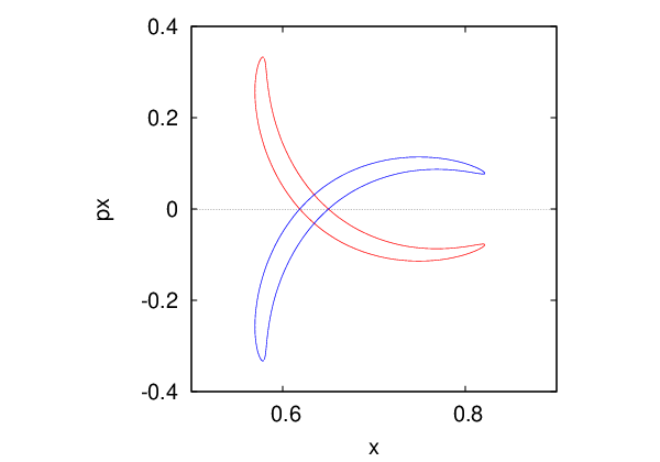
In this section we present rigorous-computer-assisted results in which we verify assumptions of Lemma 22 and thus conclude the proof of Theorem 5. For each x∈Ix\in I there are four points of intersection of Wu​(L​(x))W^{u}(L(x)) and Ws​(L​(x))W^{s}(L(x)) on {y=0}\{y=0\}. They can be seen on the left hand plot in Figure 14. We consider only the point which is furthermost to the right.

We define the set BE=[𝗑l,𝗑r]×BcB_{E}=\left[\mathsf{x}^{l},\mathsf{x}^{r}\right]\times B_{c} with 𝗑l,𝗑r\mathsf{x}^{l},\mathsf{x}^{r} chosen as

𝗑m=4.461867506615821⋅10−6,\mathsf{x}^{m}=4.461867506615821\cdot 10^{-6},
𝗑l=𝗑m−10−11,𝗑r=𝗑m+10−11.\mathsf{x}^{l}=\mathsf{x}^{m}-10^{-11},\qquad\qquad\mathsf{x}^{r}=\mathsf{x}^{m}+10^{-11}.

We verify that assumption (41) of Lemma 22 holds by computing 𝒢⁡(BEl)\mathcal{G}(B_{E}^{l}) and 𝒢⁡(BEr).\mathcal{G}(B_{E}^{r}). We plot the obtained bounds in red on the right hand side plot of Figure 14.

Next, using Remark 23 we compute

𝐚=[1.7695,1.7725],\mathbf{a}=\mathtt{[1.7695,1.7725],} (49)

hence assumption (42) of Lemma 22 holds. Applying Lemma 22 concludes the proof of Theorem 5.
Refer to caption
Refer to caption
Fig. 14: Left: Numerical sketch of Ws​(L​(x))W^{s}(L(x)) (in red) and Wu​(L​(x))W^{u}(L(x)) (in blue) intersected with {y=0}\{y=0\}. Right: we have proved that {πx,px(Wu(L(x))∩{y=0})|x∈I}\{\pi_{x,p_{x}}(W^{u}(L(x))\cap\{y=0\})|x\in I\} consists of curves which pass through two red boxes. We have also proved that their slope is between [1.7695,1.7725]\mathtt{[1.7695,1.7725]}. The blue/green line is a non-rigorous plot of the curves.

We needed to subdivide BEB_{E} into 600600 parts to compute [D​𝒢​(BE)​V+]\left[D\mathcal{G}(B_{E})V^{+}\right] together with [D​𝒢​(BE)​V−]\left[D\mathcal{G}(B_{E})V^{-}\right] with sufficient accuracy to obtain (49). Verification of assumptions of Lemma 22 took 2424 minutes on a standard laptop.

Remark 27.

From 𝐚\mathbf{a} and by SS-symmetry of manifolds Wu​(L​(x))W^{u}(L(x)) and Ws​(L​(x))W^{s}(L(x)), we obtain an estimate [58.8637∘,58.9439∘]\mathtt{[58.8637}^{\circ}\mathtt{,58.9439}^{\circ}\mathtt{]} on the angle of intersection of the curves on the x,pxx,p_{x} plane.

Remark 28.

At one go we obtain an estimate for a whole family of curves on

πx,px(Wu(L(x))∩{y=0})for x∈I.\pi_{x,p_{x}}\left(W^{u}(L(x))\cap\{y=0\}\right)\quad\text{for }x\in I.

In reality these curves are very close to each other (at furthest distance along xx of about 2.65⋅10−92.65\cdot 10^{-9}). We plotted (using non-rigorous computations) two curves which are furthest from each other on the right hand side plot of Figure 14. One is in green and the other in blue. They are visible only after a large magnification, and on a paper printout will merge together. This means that our estimate on the position of the curves is somewhat rough in comparison to non-rigorous numerical simulation.

8 Closing Remarks and Future Work

In this paper we have presented a method for proving existence of families of Lyapunov orbits in the planar restricted circular three body problem. The method gives explicit bounds on a curve of initial points, which can continue up to half the distance from L2L_{2} to the smaller primary in the Jupiter-Sun system.

We also presented a method of proving transversal intersections of invariant manifolds associated with Lyapunov orbits. The method gives explicit bounds on where the intersection takes place. It has been applied to Lyapunov orbits with energy of the comet Oterma in the Jupiter-Sun system.

In this paper we have focussed on detection of homoclinic intersections. Using identical tools one could also prove heteroclinic intersections of manifolds in the spirit of the work of Wilczak and Zgliczyński [19, 20].

Due to the fact that the presented method gives explicit estimates on the position of investigated manifolds, it is our hope to later apply it to the study of diffusion. Here is an outline of future scheme that could be followed to prove diffusion. The family of Lyapunov orbits is normally hyperbolic, hence survives time periodic perturbations. In non-autonomous setting the system no longer preserves energy, which allows for diffusion between orbits of different energies. Such mechanism has been investigated in [6] for the planar restricted elliptic three body problem, for the system with special restriction on parameters. The discussed diffusion follows from the geometric method of Delshams, de la Llave and Seara [8, 9, 10] and requires computation of Melnikov type integrals along homoclinic orbits of the PRC3BP. Since our method allows for precise and rigorous estimates for such orbits, it is our hope that such integrals could be computed using rigorous-computer assisted techniques. This combined with topological methods [5, 7] for detection of normally hyperbolic manifolds could give first rigorous results for diffusion in the three body problem with real life parameters. From this perspective, the results of this paper are a first step in a larger scheme for investigation of real life systems.

9 Acknowledgements

The author would like to thank Rafael de la Llave for discussions and remarks regarding implementation of the parameterization method. Special thanks go also to Daniel Wilczak for discussions on rigorous-computer-assisted computations using the CAPD library (http://capd.ii.uj.edu.pl).

10 Appendix

10.1 Verification of Cone Conditions

Lemma 29.

Let 𝐀\mathbf{A} be an interval matrix of the form

𝐀=(𝐚11εT𝐁𝐂)\mathbf{A}=\left(\begin{array}[c]{cc}\mathbf{a}_{11}&\mathbf{\varepsilon}^{T}\\ \mathbf{B}&\mathbf{C}\end{array}\right)

where 𝐚11=[a¯11,a¯11]\mathbf{a}_{11}=\left[\underline{a}_{11},\overline{a}_{11}\right] with a¯11>0\underline{a}_{11}>0. If for any ε∈ε\varepsilon\in\mathbf{\varepsilon}, ‖ε‖≤ϵ\left\|\varepsilon\right\|\leq\epsilon holds

a¯11−ϵ​α1+α>m,\frac{\underline{a}_{11}-\epsilon\sqrt{\alpha}}{\sqrt{1+\alpha}}>m, (50)

then for v=(𝗑,𝗒)v=(\mathsf{x},\mathsf{y}) such that Q⁡(v)=α​𝗑2−‖𝗒‖2≥0Q(v)=\alpha\mathsf{x}^{2}-\left\|\mathsf{y}\right\|^{2}\geq 0 and any A∈𝐀A\in\mathbf{A} we have ‖A​v‖>m​‖v‖.\left\|Av\right\|>m\left\|v\right\|.

Proof.

For v=(𝗑,𝗒)v=(\mathsf{x},\mathsf{y}) satisfying Q⁡(v)≥0,Q(v)\geq 0, we have ‖𝗑‖2+‖𝗒‖2≤‖𝗑‖2​(1+α).\left\|\mathsf{x}\right\|^{2}+\left\|\mathsf{y}\right\|^{2}\leq\left\|\mathsf{x}\right\|^{2}(1+\alpha). Using (50) this gives the following estimate

‖A​v‖≥a¯11​‖𝗑‖−ϵ⁡‖𝗒‖≥(a¯11−ϵ​α)​‖𝗑‖>m​‖𝗑‖2+‖𝗒‖2=m⁡‖v‖.\left\|Av\right\|\geq\underline{a}_{11}\left\|\mathsf{x}\right\|-\epsilon\left\|\mathsf{y}\right\|\geq\left(\underline{a}_{11}-\epsilon\sqrt{\alpha}\right)\left\|\mathsf{x}\right\|>m\sqrt{\left\|\mathsf{x}\right\|^{2}+\left\|\mathsf{y}\right\|^{2}}=m\left\|v\right\|.

∎

Lemma 30.

Let Q⁡(v)=Q⁡(𝗑,𝗒)=α​𝗑2−‖𝗒‖2,Q\left(v\right)=Q(\mathsf{x},\mathsf{y})=\alpha\mathsf{x}^{2}-\left\|\mathsf{y}\right\|^{2}, let CQC_{Q} be a diagonal matrix such that vT​CQ​v=Q⁡(v),v^{T}C_{Q}v=Q(v), and let 𝐀=[D​F​(Q+​(v∗))].\mathbf{A}=[DF(Q^{+}(v^{*}))]. Assume that 𝐃=𝐀𝐓​CQ​𝐀\mathbf{D=\mathbf{A}^{T}}C_{Q}\mathbf{\mathbf{A}} is an interval matrix of the form

𝐃=(𝐝11𝜺T𝜺𝐁).\mathbf{D}=\left(\begin{array}[c]{cc}\mathbf{d}_{11}&\boldsymbol{\varepsilon}^{T}\\ \boldsymbol{\varepsilon}&\mathbf{B}\end{array}\right).

Assume that 𝐝11=[d¯11,d¯11]\mathbf{d}_{11}=\left[\underline{d}_{11},\overline{d}_{11}\right] with d¯11>0\underline{d}_{11}>0 and that for some M>0,M>0, for any symmetric matrix B∈𝐁B\in\mathbf{B}

inf{λ|λ∈spec⁡(B)}>−M.\inf\left\{\lambda|\lambda\in\mathrm{spec}\left(B\right)\right\}>-M. (51)

If for any ε∈𝛆\varepsilon\in\boldsymbol{\varepsilon} we have ‖ε‖≤ϵ\left\|\varepsilon\right\|\leq\epsilon and d¯11−2​ϵ>M​α\underline{d}_{11}-2\epsilon>M\alpha, then for any v1,v2∈U,v_{1},v_{2}\in U, v1≠v2v_{1}\neq v_{2} such that Q⁡(v1−v2)≥0Q\left(v_{1}-v_{2}\right)\geq 0

Q⁡(F⁡(v1)−F⁡(v2))>0.Q\left(F(v_{1})-F(v_{2})\right)>0.
Proof.

By (33) Q⁡(F⁡(v1)−F⁡(v2))=(v1−v2)T​D​(v1−v2)Q\left(F(v_{1})-F(v_{2})\right)=\left(v_{1}-v_{2}\right)^{T}D\left(v_{1}-v_{2}\right) for some symmetric matrix D∈𝐃D\in\mathbf{D}.

For v=(𝗑,𝗒)v=\left(\mathsf{x},\mathsf{y}\right) such that Q⁡(𝗑,𝗒)≥0Q(\mathsf{x},\mathsf{y})\geq 0 and for any symmetric D∈𝐃D\in\mathbf{D}

D=(d11εTεB)D=\left(\begin{array}[c]{cc}d_{11}&\varepsilon^{T}\\ \varepsilon&B\end{array}\right)

we compute the following bounds

vT​A​v\displaystyle v^{T}Av =d11​𝗑2+𝗑​εT​𝗒+𝗒T​ε​𝗑+𝗒T​B​𝗒\displaystyle=d_{11}\mathsf{x}^{2}+\mathsf{x}\varepsilon^{T}\mathsf{y}+\mathsf{y}^{T}\varepsilon\mathsf{x}+\mathsf{y}^{T}B\mathsf{y}
≥d¯11​𝗑2−2​ϵ​‖𝗒‖​|𝗑|−M​‖𝗒‖2\displaystyle\geq\underline{d}_{11}\mathsf{x}^{2}-2\epsilon\left\|\mathsf{y}\right\|\left|\mathsf{x}\right|-M\left\|\mathsf{y}\right\|^{2}
≥(d¯11−2​ϵ)​𝗑2−M​‖𝗒‖2\displaystyle\geq\left(\underline{d}_{11}-2\epsilon\right)\mathsf{x}^{2}-M\left\|\mathsf{y}\right\|^{2}
=M⁡(d¯11−2​ϵM​𝗑2−‖𝗒‖2)\displaystyle=M\left(\frac{\underline{d}_{11}-2\epsilon}{M}\mathsf{x}^{2}-\left\|\mathsf{y}\right\|^{2}\right)
>M​Q​(𝗑,𝗒)\displaystyle>MQ\left(\mathsf{x},\mathsf{y}\right)
>0.\displaystyle>0.

∎

Remark 31.

Assumption (51) is easily verifiable from Gershgorin theorem.

10.2 Bounds for the Images in Local Coordinates

Here we give a proof of Lemma 17.

Proof.

Inclusion (39) is equivalent to showing that for any τ∈𝐓,\tau\in\mathbf{T,} and any v1∈U1v_{1}\in U_{1} there exists an v2v_{2}\mathbf{\ }in U2U_{2} such that

G⁡(τ,v1,v2)=0.G(\tau,v_{1},v_{2})=0. (52)

Let us fix a τ∈𝐓\tau\in\mathbf{T} and v1∈U1v_{1}\in U_{1} and use a notation Gτ,v1​(v2)=G⁡(τ,v1,v2)G_{\tau,v_{1}}(v_{2})=G(\tau,v_{1},v_{2}). Observe that [D​Gτ,v1​(U2)]⊂𝐀⁡(U2)\left[DG_{\tau,v_{1}}(U_{2})\right]\subset\mathbf{A}(U_{2}) and [Gτ,v1​(v0)]⊂[G⁡(𝐓,U1,v0)].\left[G_{\tau,v_{1}}(v_{0})\right]\subset\left[G(\mathbf{T},U_{1},v_{0})\right]. Since from (38)

v0−[D​Gτ,v1​(U2)]−1​Gτ,v1​(v0)⊂N⁡(𝐓,v0,U1,U2)⊂U2,v_{0}-\left[DG_{\tau,v_{1}}(U_{2})\right]^{-1}G_{\tau,v_{1}}(v_{0})\subset N(\mathbf{T},v_{0},U_{1},U_{2})\subset U_{2},

by the interval Newton method (Theorem 1) there exists a unique v2=v2​(τ,v1)∈U2,v_{2}=v_{2}\left(\tau,v_{1}\right)\in U_{2}, which satisfies (52). ∎

Remark 32.

When applying Lemma 17, due to very strong hyperbolicity of the map Φτ\Phi_{\tau} it pays off to use the mean value theorem. Taking U1=v1+BU_{1}=v_{1}+B we can compute

N⁡(𝐓,v0,U1,U2)=v0−[𝐀⁡(U2)]−1​G​(𝐓,v1,v0)−[(𝐀​(U2)−1​∂G∂v1​(𝐓,U1,v0))​B].N(\mathbf{T},v_{0},U_{1},U_{2})=v_{0}-\left[\mathbf{A}\left(U_{2}\right)\right]^{-1}G(\mathbf{T},v_{1},v_{0})-\left[\left(\mathbf{A}\left(U_{2}\right)^{-1}\frac{\partial G}{\partial v_{1}}(\mathbf{T},U_{1},v_{0})\right)B\right].

This is a better form since in (below we neglect arguments in order to keep the formula compact)

𝐀−1∂G∂v1=−Dλ−1⋅((Dψ)−1⋅DΦ~τ⋅Dψ),\mathbf{A}^{-1}\frac{\partial G}{\partial v_{1}}=-D\lambda^{-1}\cdot\left(\left(D\psi\right)^{-1}\cdot D\tilde{\Phi}_{\tau}\cdot D\psi\right), (53)

the strong hyperbolic expansion cancels out. This is the main advantage of Lemma 17.

Here we give a technical lemma that can be used for computation of

ψ−1​(C−1​((x,0,0,κ⁡(x))−q0))for ​x∈I\psi^{-1}(C^{-1}\left((x,0,0,\kappa(x))-q^{0}\right))\quad\text{for }x\in I

and q0=(x0,0,0,py0)q^{0}=(x^{0},0,0,p_{y}^{0}). Below, RR can be any matrix close to D​ψ−1​(0)​C−1​AD\psi^{-1}(0)C^{-1}A.

Lemma 33.

Let a∈ℝa\in\mathbb{R} and J1⊂ℝJ_{1}\subset\mathbb{R} be from Lemma 2 and let

A=(100001000010a001).A=\left(\begin{array}[c]{llll}1&0&0&0\\ 0&1&0&0\\ 0&0&1&0\\ a&0&0&1\end{array}\right).

Let 𝐁\mathbf{B} be a set in ℝ4\mathbb{R}^{4}, let RR be a 4×44\times 4 matrix and let

M:=[A−1​P​D​ψ​(R​𝐁)​R]−1​(I−x0,0,0,J1−py0).M:=\left[A^{-1}PD\psi\left(R\mathbf{B}\right)R\right]^{-1}\left(I-x^{0},0,0,J_{1}-p_{y}^{0}\right)\mathbf{.}

If

M⊂𝐁M\subset\mathbf{B} (54)

then ψ−1​(C−1​((x,0,0,κ⁡(x))−q0))⊂R​𝐁\psi^{-1}(C^{-1}\left((x,0,0,\kappa(x))-q^{0}\right))\subset R\mathbf{B}.

Proof.

By Lemma 2

(x,0,0,κ⁡(x))\displaystyle\left(x,0,0,\kappa(x)\right) ∈(x0,0,0,py0)+(I−x0,0,0,a⁡(I−x0)+J1−py0)\displaystyle\in(x^{0},0,0,p_{y}^{0})+\left(I-x^{0},0,0,a(I-x^{0})+J_{1}-p_{y}^{0}\right)
=q0+A⁡(I−x0,0,0,J1−py0),\displaystyle=q^{0}+A\left(I-x^{0},0,0,J_{1}-p_{y}^{0}\right),

hence

(x,0,0,κ⁡(x))−q0∈A⁡(I−x0,0,0,J1−py0).(x,0,0,\kappa(x))-q^{0}\in A\left(I-x^{0},0,0,J_{1}-p_{y}^{0}\right). (55)

Let

Gq​(p)=A−1​C​ψ​(R​p)−qG_{q}(p)=A^{-1}C\psi(Rp)-q

If we can show that for any q∈(I−x0,0,0,J1−py0)q\in\left(I-x^{0},0,0,J_{1}-p_{y}^{0}\right) there exists a p∈𝐁p\in\mathbf{B} such that

Gq​(p)=0G_{q}(p)=0 (56)

then

ψ−1​(C−1​A​q)=R​p,\psi^{-1}\left(C^{-1}Aq\right)=Rp,

hence by (55)

ψ−1​(C−1​((x,0,0,κ⁡(x))−q0))⊂R​𝐁.\psi^{-1}(C^{-1}\left((x,0,0,\kappa(x))-q^{0}\right))\subset R\mathbf{B.}

To show (56) we apply the interval Newton method (Theorem 1). Since ψ⁡(0)=0\psi(0)=0 we can compute

N⁡(0,𝐁)\displaystyle N(0,\mathbf{B}) =−[dd​p​Gq​(𝐁)]−1​Gq​(0)\displaystyle=-\left[\frac{d}{dp}G_{q}(\mathbf{B})\right]^{-1}G_{q}(0)
=−[A−1​C​D​ψ​(R​𝐁)​R]−1​(−q)\displaystyle=-\left[A^{-1}CD\psi(R\mathbf{B})R\right]^{-1}\left(-q\right)
⊂M,\displaystyle\subset M,

and by (54) combined with Theorem 1 obtain (56), and hence obtain our claim. ∎

References

  • [1] R. Abraham, J. Marsden, Foundations of mechanics. Benjamin/Cummings Publishing Co., Inc., Advanced Book Program, Reading, Mass. (1978).
  • [2] G. Alefeld, Inclusion methods for systems of nonlinear equations - the interval Newton method and modifications. Topics in validated computations (Oldenburg, 1993), 7–26, Stud. Comput. Math., 5, North-Holland, Amsterdam, 1994.
  • [3] R. Broucke. Periodic orbits in the restricted three–body problem with Earth–Moon masses. NASA–JPL technical report 32-1168 (1968), available at: ntrs.nasa.gov/archive/nasa/casi.ntrs.nasa.gov/19680013800_1968013800.pdf.
  • [4] X. Cabré, E. Fontich, R. de la Llave, The parameterization method for invariant manifolds. III. Overview and applications. J. Differential Equations 218 (2005), no. 2, 444–515.
  • [5] M. J. Capiński, P. Roldán, Existence of a Center Manifold in a Practical Domain around L1L_{1} in the Restricted Three Body Problem, to appear in SIADS.
  • [6] M. J. Capiński and Piotr Zgliczyński. Transition tori in the planar restricted elliptic three-body problem Nonlinearity, 24:1395–1432, 2011.
  • [7] M. J. Capiński and Piotr Zgliczyński. Cone conditions and covering relations for topologically normally hyperbolic manifolds. Discrete Contin. Dyn. Syst., 30(3):641–670, 2011.
  • [8] A. Delshams, R.de la Llave, T. Seara, A geometric approach to the existence of orbits with unbounded energy in generic periodic perturbations by a potential of generic geodesic flows of T2. Comm. Math. Phys. 209 (2000), no. 2, 353–392.
  • [9] A. Delshams, D. de la Llave, T. Seara, A geometric mechanism for diffusion in Hamiltonian systems overcoming the large gap problem: heuristics and rigorous verification on a model. Mem. Amer. Math. Soc. 179 (2006), no. 844,
  • [10] A. Delshams, D. de la Llave, T. Seara, Geometric properties of the scattering map of a normally hyperbolic invariant manifold. Adv. Math. 217 (2008), no. 3, 1096–1153.
  • [11] G. Gómez, À. Jorba, C. Simó, and J. Masdemont. Dynamics and mission design near libration points. Vol. III, volume 4 of World Scientific Monograph Series in Mathematics. World Scientific Publishing Co. Inc., River Edge, NJ, 2001. Advanced methods for collinear points.
  • [12] G. Gómez, W. S. Koon, M. W. Lo, J. E. Marsden, J. Masdemont, and S. D. Ross. Connecting orbits and invariant manifolds in the spatial restricted three-body problem. Nonlinearity, 17(5):1571–1606, 2004.
  • [13] À. Jorba and C. Simó. Effective stability for periodically perturbed Hamiltonian systems in Hamiltonian mechanics (Toruń, 1993), volume 331 of NATO Adv. Sci. Inst. Ser. B Phys., pages 245–252. Plenum, New York, 1994.
  • [14] À. Jorba and J. Villanueva. Numerical computation of normal forms around some periodic orbits of the restricted three-body problem. Phys. D, 114(3-4):197–229, 1998.
  • [15] W. Koon, M. Lo, J. Marsden and S. Ross, Heteroclinic connections between periodic orbits and resonance transitions in celestial mechanics Chaos 10 (2000), 427–69
  • [16] J. Llibre, R. Martinez, C. Simó,Transversality of the Invariant Manifolds Associated to the Lyapunov Family of Periodic Orbits Near L2L_{2} in the Restricted Three Body Problem, Journal of Differential Equations 58 (1985), 104-156.
  • [17] Jürgen Moser. On the generalization of a theorem of A. Liapounoff. Comm. Pure Appl. Math., 11:257–271, 1958.
  • [18] C. L. Siegel and J. K. Moser. Lectures on celestial mechanics. Classics in Mathematics. Springer-Verlag, Berlin, 1995. Translated from the German by C. I. Kalme, Reprint of the 1971 translation.
  • [19] D. Wilczak, P. Zgliczyński, Heteroclinic Connections between Periodic Orbits in Planar Restricted Circular Three Body Problem - A Computer Assisted Proof, Comm. Math. Phys. 234 (2003) 1, 37-75,
  • [20] D. Wilczak, P. Zgliczyński, Heteroclinic Connections between Periodic Orbits in Planar Restricted Circular Three Body Problem - Part II , Comm. Math. Phys. 259, 561-576 (2005),
  • [21] P. Zgliczyński, Covering relations, cone conditions and the stable manifold theorem. J. Differential Equations 246 (2009), no. 5, 1774–1819.