Antlia Dwarf Galaxy: Distance, quantitative morphology and recent formation history via statistical field correction
Abstract
We apply a statistical field correction technique originally designed to determine membership of high redshift galaxy clusters to Hubble Space Telescope imaging of the Antlia Dwarf Galaxy; a galaxy at the very edge of the Local Group. Using the tip of the red giant branch standard candle method coupled with a simple Sobel edge detection filter we find a new distance to Antlia of Mpc. For the first time for a Local Group Member, we compute the concentration, asymmetry and clumpiness (CAS) quantitative morphology parameters for Antlia from the distribution of resolved stars in the HST/ACS field, corrected with a new method for contaminants and complement these parameters with the Gini coefficient () and the second order moment of the brightest 20 per cent of the flux (). We show that it is a classic dwarf elliptical (, , , and in the F814W band), but has an appreciable blue stellar population at its core, confirming on-going star-formation. The values of asymmetry and clumpiness, as well as Gini and are consistent with an undisturbed galaxy. Although our analysis suggests that Antlia may not be tidally influenced by NGC 3109 it does not necessarily preclude such interaction.
Keywords:
methods: statistical — stars: Hertzsprung-Russell and colour-magnitude diagrams — Local Group — galaxies: individual: Antlia Dwarf Galaxy — galaxies: distances and redshifts — galaxies: structure1 Introduction
In the successful hierarchical cold dark matter paradigm, galaxies grow through repeated mergers with other galaxies (e.g. Guo & White 2008; De Lucia & Blaizot 2007; White & Rees 1978). Inside this hierarchy, the dwarf galaxy sits at the bottom; analogous to a fundamental galaxy ‘building block’ that can be combined with other blocks in a large variety of ways (cf. Durhuus & Eilers 2005). Indeed, in the local Universe, both the Milky Way and Andromeda are observed to still be under-going construction due to the accretion of such dwarf galaxies (Martin et al. 2004; Ibata et al. 2001). Further, the Milky Way, Andromeda and M33 seem to be the few galaxies in the Local Group that are not dwarfs – Mateo (1998) reports that there are likely in excess of 40 bona fide dwarf galaxy members of the Local Group (see also Grebel 1997).
Dwarf galaxies are not only the basic building block for galaxy evolution, but they are also the most numerous across all redshifts (Marzke & Da Costa 1997; Ferguson & Binggelli 1994). The Local Group presents a solid test bed for studying the varied properties of dwarf galaxies. Often, they appear to have had strong (sometimes on-going) star-formation whose origin is somewhat enigmatic (Mateo 1998 and references therein) but probably triggered by recent (tidal) interactions with their close neighbours (see Tolstoy, Hill & Tosi 2009 for a detailed review; Lewis et al. 2007). Mateo (1998) further point out that it is the case that no two Local Group dwarfs have the exact same star-formation history (see also Koleva et al. 2009; Weisz et al. 2011).
In the present work, we focus on the Antlia Dwarf Galaxy with the broad aims of discerning its distance, morphology and recent star-formation history through the use of an extensively used extra-galactic contamination subtraction technique (Pimbblet et al. 2002) and a quantitative morphology approach (Conselice 2003).
Although Antlia was noted by Corwin, de Vaucouleurs & de Vaucouleurs (1985) as a possible local dwarf galaxy, it was Whiting, Irwin & Hau (1997) who published its distance for the first time and confirmed it as being a probable member of the Local Group. Whiting et al. (1997) suggest that Antlia is a ‘typical’ dwarf elliptical galaxy, reminiscent of the Tucana dwarf and the various Milky Way satellites. More recent publications suggest that Antlia is anything but a regular dwarf elliptical, with a strong blue stellar component and on-going star-formation (e.g. Aparicio et al. 1997; Sarajedini et al. 1997; Piersimoni et al. 1999; Dalcanton et al. 2009; McQuinn et al. 2010). McQuinn et al. (2010) made a study of the star-formation histories of 18 dwarf galaxies that appear to be under-going star-bursts. Taking data from the Hubble Space Telescope (HST) archive, they suggest that the majority of their sample is still under-going present-day starbursts, whilst 30 per cent have indicators of ‘fossil’ star-bursting within the past few hundred Myr or so. Amongst those with a fossil burst, McQuinn et al. (2010) note that the Antlia Dwarf Galaxy has both the lowest mass and star-formation rate in their sample. However, set against the context of its own history, the fossil burst in Antlia is both significant and observationally measurable. Yet, this galaxy would not be considered to have a significant star-formation rate from a simple analysis of its archival ground-based imaging.
Antlia presents an unique target since it is located on the edge of the Local Group and may have had relatively few interactions with other group members; its nearest neighbour being NGC 3109. Given the distance between these two galaxies may be as large as 180 kpc and their relative velocity 45 km s-1 (Aparicio et al. 1997), it is unlikely they are gravitationally bound and interacting at present. But if the distance difference is much lower, (e.g. 28 kpc due to them being at the same radial distance; Aparicio et al. 1997), then it may be the case that Antlia is a satellite of NGC 3109 (as suggested by van den Bergh 1999) and have had historic interactions with it. Newer measurements of the distance to Antlia (Dalcanton et al. 2009) suggest that it could be much further away – perhaps over 300 kpc. Yet, a number of authors suggest that warping in the disk of NGC 3109 may be due to interaction with Antlia (Lee, Grebel & Hodge 2003; Grebel, Gallagher & Harbeck 2003; Barnes & de Blok 2001; Jobin & Carignan 1990). Our approach to determining Antlia’s quantitative morphology will help address both its distance and recent evolution.
The format of this work is as follows. In Section 2, we detail the HST dataset that is used in this work and indicate how we sample the stellar contaminants. In Section 3, we fully detail the contamination correction technique of Pimbblet et al. (2002) and how we modify it to be better suited to the present case. To calculate the distance to Antlia, we employ a tip of the red giant branch standard candle method in Section 4. Section 5 details our investigation of the morphology of Antlia using the Conselice (2003) CAS parameters, as well as the Gini and parameters, and we summarize our findings in Section 6.
2 Data
In this work, we utilize the archival HST F814W and F606W passband observations (i.e. a single colour) that have been processed by the Advanced Camera for Surveys (ACS) Nearby Galaxy Treasury Survey (ANGST) of Dalcanton et al. (2009) from an original survey by Tully et al. (2006). Here, we summarize the pertinent points from Dalcanton et al. (2009) concerning the ANGST data pipeline and refer the reader to that article for a full description and treatment. ANGST is more than an HST imaging survey: systematic object detection, classification and quality control checks have been implemented uniformly across legacy images of nearby galaxies.
Following standard image reduction steps (flat fielding, bias subtraction), photometry is performed with the dolphot package (Dolphin 2000). The package aligns the stars contained in the ACS images to a high precision ( arcsec) and calculates a local point spread function for each star from Tiny Tim (Krist 1995). The flux (and hence magnitude) for each star is then determined in an iterative process by calculating the flux arising from each star in the crowded field. The final catalogue is then culled of objects of low ‘sharpness’ (i.e. probable galaxies) and stars from highly crowded regions whose photometry may be significantly compromised.
The resultant multi-colour photometry catalogues are publically available at www.nearbygalaxies.org. ANGST reaches several magnitudes below the expected tip of the red giant branch that we will use in Section 4 to determine the distance to Antlia with and is therefore ideal for our work. An image of the ACS observations of Antlia is shown in Fig. 1. From ANGST, we use only those stars that have passed the quality cuts for sharpness and crowding (see Dalcanton et al. 2009).
We now divide the data up into three samples (see Fig. 1): an inner sample (covering the very centre of the galaxy and the highest stellar density regimes; deg); an outer sample (at larger radii from the galaxy centre and lower stellar densities; deg); and a ‘field’ sample (where we assume the contribution from the Antlia Dwarf Galaxy is minimized and the majority of the stars are likely foreground Milky Way stars; deg). These divisions provide broad analogues of divisions made by Aparicio et al. (1997) and will facilitate comparison in order to test (e.g.) the presence of a blue stellar core. Most of the analysis in this work will concentrate on the inner sample and we display a schematic of these divisions in Fig. 1. We note that we intentionally build in a small buffer zone between the outer sample and the field sample.

3 Contamination subtraction
At bright magnitudes (F814W), it is likely that of the order 10’s of Milky Way stars contaminate the colour-magnitude diagram for the Antlia Dwarf Galaxy (Aparicio et al. 1997). As one proceeds to fainter magnitudes, the errors in the photometry increase and we may expect a higher proportion of stars could be interlopers. In order to correct this foreground contamination, we follow the statistical method of Pimbblet et al. (2002) to generate artificial star counts to correct for contamination. Although the method was originally developed to tackle galaxy clusters at modest redshifts, the concept underlying the correction technique is identical in the present case and has been utilized & emulated extensively in the literature (e.g. Tanaka et al. 2005; Wake et al. 2005; Rudnick et al. 2009; Urquhart et al. 2010). Here, we outline the pertinent details of the procedure.

Each of the three samples are firstly represented on a colour-magnitude grid. We can then compute the probability of a given object at a particular grid location being a field object (i.e. a contaminant) as
| (1) |
where is an areal scaling factor that matches the size of the field sample to that of either the inner or outer samples. In this work, we deviate from the original Pimbblet et al. (2002) formulation by taking care of through perturbing the field sample. This is achieved adding in extra ‘field’ objects to the field sample until the area covered matches that of the inner or outer samples (assuming a fixed stellar density for the field sample). We do this by randomly selecting an object from the field sample and modifying its colour and magnitude by a random Gaussian deviation multiplied by the errors on both colour and magnitude (respectively). This is repeated until the area of the field sample matches that of the inner or outer samples, as required. The reason that we choose this approach rather than simply use a factor, , to scale the probability by is due to the coverage of the field sample itself being only modest in size. Ideally, we would use an extensive suite of field observations that are close to the target (Antlia) so that gross fluctuations in the stellar foreground do not affect the sample. In the present case, this is the only HST data that is available near to Antlia11 1 A search with the high-level science archive (hla.stsci.edu) shows that although there are other fields within 10 degrees of Antlia with the correct combination of filters, none of them constitute a more appropriate field sample as they are primarily targeted on other large, nearby galaxies. and we therefore argue that perturbing the field sample in this manner is more desirable and representative than just applying the scaling. Once the field sample is area-scaled, is computed for each grid in the colour-magnitude plane, using bin sizes of 0.5 in (F606W-F814W) and 1.0 in F814W magnitude.
gives us the probability of an object at a particular location on the colour-magnitude plane of being a contaminant. We use this to determine which objects are members of Antlia by generating a random number and comparing it to for each star. If the random number is less than , then it is classed as a contaminant and thrown out. An illustrative example of this method is depicted in Fig. 2 where we display the colour-magnitude plane of the original inner and outer samples, an area-matched field sample and the resultant colour-magnitude diagram after the field correction. As can be seen, relatively few are removed from the critical region near the tip of the red giant branch, whilst 100’s to 1000’s are removed at both fainter magnitudes and redder colours. Already we can see that Antlia possesses a significant population of blue stars and is under-going recent and / or present-day star-formation (cf. Aparicio et al. 1997). Moreover, the bluer stars are largely confined to the inner sample whereas the outer sample largely lacks this population. This qualitative observation supports the findings of previous works (Aparicio et al. 1997; McQuinn et al. 2010) and means that they are not adversely affected by stellar contamination.
The statistical field correction is repeated 100 times in a Monte-Carlo fashion for both the inner and outer samples to give better statistics for this work. However, it is apparent from Fig. 2 that a large number of objects are removed in comparison to models of the Milky Way’s stellar distribution (Robin et al. 2003). Part of this may be intrinsic to the methodology employed and choice of field sample. By this, we mean that there are likely stars from Antlia contained in the field sample and will therefore be part of the subtraction. Ryś et al. (2011) show that red giant stars in the outer halo of other dwarf galaxies are well fit by a de Vaucouleurs profile. Using such a profile, at the radii of the field sample we would expect 0–1 Antlia stars arcmin-2 to be present, which at worst would correspond to stars. Given the constraints of the data, we are happy to live with this level of self-contamination.
However, there may be further contamination from other sources (i.e. background galaxies). Given that galaxy profiles are generally very different from stellar profiles, we are confident that the ANGST pipeline results in only small contamination from galaxies for our study at bright magnitudes. But there could certainly be an appreciable population of (unresolved) galaxies that masquerade as stars – especially at faint magnitudes (cf. Radburn-Smith et al. 2011). To be confused with a star, a background galaxy would have to have a light profile similar to a compact dwarf galaxy (cf. Gregg et al. 2003; Drinkwater et al. 2003). In the absence of redshifts, it is practically impossible to differentiate such galaxies from stars. Alternatively, an unresolved galaxy can be readily confused with a star simply by being near to the photometric limit. This type of contaminant would account for the majority of the low magnitude “stars” that are subtracted. Since we’re using a statistical correction, such galaxies should be properly subtracted assuming that there are no large galaxy clusters in the background.
We contend that within the limits of our chosen method and field sample, the large number of objects removed will have minimal impact on the parameters of merit (e.g. distance) that we will derive below.
4 Tip of the Red Giant Branch
The tip of the red giant branch (TRGB) is an excellent indicator of galaxy distance if one can resolve individual stars inside a given target galaxy (Lee, Freedman & Madore 1993; see also Madore & Freedman 1998 and references therein). Since the tip of the red giant branch represents the first ascent (core helium flash) of red giant branch, the method is analogous to finding standard candles in nearby galaxies. Use of HST imaging combined with this method has directly lead to accurate determinations of distances to nearby systems ranging from the Large Magellanic Cloud (Romaniello et al. 2000) to NGC 300 (Rizzi et al. 2006) and beyond (Dalcanton et al. 2009; Radburn-Smith et al. 2011).
One of the strengths of the method is its simplicity: the key observable is to determine the -band magnitude of the red giant branch where the luminosity function is abruptly truncated. At -band wavelengths, the dependence of this position along the luminosity function is largely independent of metallicity (Da Costa & Armandroff 1990). Further, the TRGB magnitude is only expected to vary by mag over a large range of of ages (2–15 Gyr; Iben & Renzini 1983). Although the TRBG was determined by eye in its early days (e.g. Mould & Kristian 1986), a straight-forward edge detection technique (e.g. Sakai, Madore & Freedman 1996; see also Méndez et al. 2002) is now more frequently applied to the data to determine the position of the tip.
There are many approaches to edge detection, ranging from the Canny (1986) algorithm, Laplacian edge detection, to more complex methodologies (e.g. Frayn & Gilmore 2003; Méndez et al. 2002). In general, the task of edge detection is a non-trivial endeavour due to how data is binned and noise properties present. In astronomical imaging and two dimensional edge detection problems, there are a wide range of edge detection approaches employed for various ends such as cosmic ray detection and rejection (e.g. Laplacian edge detection; see Farage & Pimbblet 2005; van Dokkum 2001) and morphological measurements to differentiate stars from galaxies (e.g. the mathematical morphology gradient operator; see Moore, Pimbblet & Drinkwater 2006). Considering the high quality of the colour magnitude diagrams (Fig. 2), the standard Sobel filter approach (Lee et al. 1993) is sound enough for this work (Svalbe, priv. comm.).
For each of the realizations of the contamination correction technique (Fig 2), we now compute the position of the -band (i.e. F814W band) TRGB by creating a luminosity function and passing a Sobel filter with a kernel of [-2,-1,0,+1,+2] across it. The luminosity function is limited to (F606W-F814W) to curtail the influence of non-red-giant stars on the resultant TRGB measurement. This kernel is in keeping with Lee et al. (1993; see also Sakai et al. 1996) and will yield a maximum value for the greatest count discontinuity. An example of the application of this filtering technique is displayed in Fig. 3.

We now apply this method to all of field subtracted realizations of the Antlia colour magnitude diagram. We find a raw (i.e. not extinction corrected) for the inner sample, whereas the outer sample yields where the quoted error is the standard deviation from the 100 realizations. The difference between the inner and outer samples is likely due to extinction (cf. Holwerda et al. 2009 who report a few tenths mag extinction in the outer regions of more massive galaxies).
Using the approach of Méndez et al. (2002), Dalcanton et al. (2009) report a raw – using the same HST dataset, the only difference being that they employ the full field of view and avoided the highly crowded parts of Antlia – less than away from the value that we derive for the inner sample. We note that Dalcanton et al. (2009) also perturbed the stellar data points by a Guassian random error in Monte Carlo trials to obtain their result. This suggests that the more complex approach of Méndez et al. (2002) who Gaussian smooth the luminosity function prior to applying a continuous logarithmic edge detection (a subtle modification of the Sakai et al. 1996 approach) does not dramatically improve the computation of . This is likely due to the fact that this bright part of the colour magnitude diagram is not significantly affected by noise. Following Dalcanton et al. (2009; inparticular using the extinction and absolute value; from Table 5), we compute a distance of Mpc to Antlia.
From a search of the NASA/IPAC Extragalactic Database (NED), our results are completely congruous with Dalcanton et al. (2009) who themselves derive a distance of Mpc to Antlia and the earlier studies of Aparicio et al. (1997) who report Mpc, van den Bergh (1999) at Mpc, Blitz & Robishaw (2000) with Mpc, and Tully et al. (2006) with 1.25 Mpc22 2 Tully et al. (2006) do not quote an error on Antlia’s distance. However, they do quote , which would produce an error on their distance that is bigger than ours by a factor of 2–3.. However, it is somewhat smaller than the value of Mpc reported by Piersimoni et al. (1999) who obtained from ground-based observations; although the amount of dust affecting the galaxy may be significant and cause the distance estimate to vary by as much as 0.1 Mpc (see Sarajedini, Claver, & Ostheimer 1997 who quote a range of distances from 1.24 to 1.33 Mpc depending on the amount of dust present). Finally, we note that Whiting, Irwin & Hau (1997) found a distance of Mpc which seems the most discrepant distance in the literature. We suggest the depth and photometric accuracy of HST is a prime factor in the difference to this earlier analysis.
We note that our distance places Antlia over 300 kpc from NGC 3109, thereby implying little present interaction.
5 Morphology of Antlia
Motivated by tying together the structure of a galaxy to its formation and evolutionary history, the use of quantitative morphology has bloomed over the past few decades. One of the most widely adopted (and straight forward) approaches to quantitative galaxy morphology is the use of the model-independant ‘CAS’ paradigm (Conselice 2003; see also Conselice 2006 and references therein). We also make use of the non-parametric Gini () and coefficients (see Lotz et al. 2004) to complement the CAS paradigm. Before we compute the CAS values, we must first turn the contamination corrected realizations of Antlia stars in to new images.
5.1 Image Creation
Each realization of Antlia resulting from our correction technique contains both (RA,Dec) and the HST pixel (x,y) positions. In principle, we can simply bin up these positions to create a new image of Antlia for each contamination-corrected realization. But as Fig. 4 demonstrates, there are several issues to deal with in binning up the image.
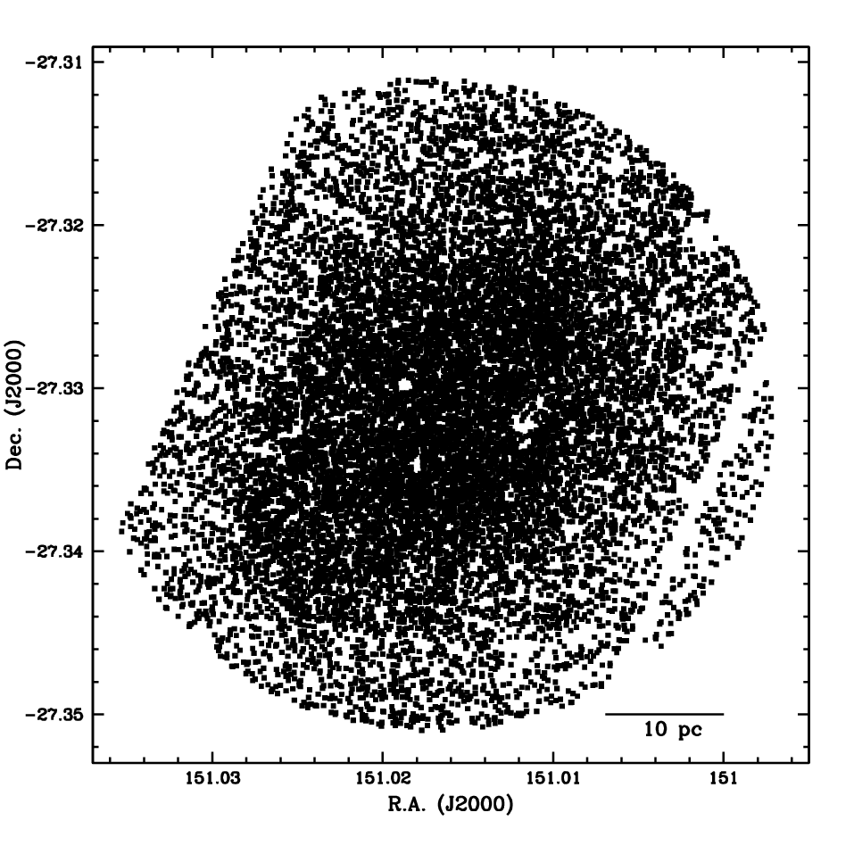
Firstly, there is a very obvious gap between the HST chips, as well as an edge on the opposite side. Secondly, there are clear holes in the stellar distribution due to large, saturated stars in the original HST image (cf. Fig. 1) Thirdly, the data need to be binned up into larger pixels, but the exact amount of binning required is unclear.
We tackle the latter question first. When the original CAS parameters were tested out, they were applied to and benchmarked against the Frei et al. (1996) dataset (Bershady et al. 2000; Conselice 2003; see also Conselice et al. 2000). The Frei et al. (1996) sample consists of 113 nearby galaxies imaged in multiple pass-bands from ground based telescopes, with various auxiliary data available (Conselice et al. 2000). Therefore, it makes logical sense to attempt to bin up our data so that it appears to be at the same distance as these benchmark galaxies. From Fig. 4 and Table 1 of Frei et al. (1996), the mean heliocentric recession velocity of the sample is a little above kms-1. Given our calculation of the distance to Antlia above, we would have to move Antlia outward by a factor of to match its physical scale to angular size ratio to that of a typical Frei et al. (1996) galaxy. Rounding down, this yields pixels to fit the points displayed in Fig. 4 into. To populate the bins, we weigh each pixel proportional to the brightness of the stars contained within (Fig. 5).
To ensure that chip edge effects are minimized, we replace all pixel values that were set at zero with a random value scattered about the mean of the pixel values in the edge regions. This makes the edges of the inner sample blend in with surrounding noise. Finally, to take care of the holes in the pixel distribution due to the saturated stars near the centre of the stellar distribution, we draw values from nearby populated pixels to interpolate over then. An example of one of the images this process produces can be seen in Fig. 6. In this image, the 100 pixels cover pc at the TRGB distance of Antlia. This process is performed for both the F814W and F606W bands. We suggest that this resultant image is sufficient for the subsequent application of the CAS quantitative morphology algorithms.

5.2 Concentration ()
The first of the CAS parameters that we measure is the concentration of the galaxy, . Central light concentration can be measured in a variety of ways (e.g. Kent 1985; Abraham et al. 1994), but each provides sensitivity to different galaxy morphological populations (Conselice 2003) and can readily be used for star-galaxy differentiation (e.g. Pimbblet et al. 2001). We follow Conselice (2003) and Bershady et al. (2000) and define
| (2) |
where and is 80% and 20% of the curve of growth radii (Bershady et al. 2000; see also Petrosian 1976; Wirth, Koo & Kron 1994).
For our 100 realizations of Antlia, we find that for F814W and for F606W (where the quoted error is the standard deviation of from the 100 realizations). This is a remarkably low central concentration, amongst the lowest values produced through this method (for comparison, elliptical galaxies tend to give whereas disk dominated galaxies produce values in the range for band images which sits between the F814W and F606W bands; Conselice 2003). Conselice (2003) suggest that this value may be consistent with irregular galaxies, very late disk types, as well as dwarf elliptical galaxies.
5.3 Asymmetry ()
The second CAS parameter, asymmetry is a very straight forward measure of how symmetric the galaxy is. Formally, we follow Conselice (2003) and define it as
| (3) |
where is the original image, and is rotated through 180 degrees about its centre. Both and around found by summing over all pixel values in the image. has been shown to correlate well with both morphological type and colour of a galaxy (Conselice et al. 2000; Conselice 2003) with lower values denoting both redder colours and morphologically earlier types. We refer the reader to Conselice (2003) for more detail about this parameter.
There are usually issues with its derivation that are noteworthy, however. Firstly, the exact choice of the centre of the image can result in dramatic changes to the value of – Conselice et al. (2000) report that even a 1 per cent shift of the centre can cause per cent change in . The usual manner to cope with this is to find which of the 8 pixels surrounding the nominal central pixel has the minimum value of . In this work, we use the luminosity-weighted centre of Antlia quoted by Whiting et al. (2007). This should be accurate to within less than ’ (i.e. sub-pixel accuracy in our binned up image) and adequate for our purposes.
The second main issue with the computation of is background subtraction. Typically one needs to sample a nearby ‘blank’ region and subtract off the nominal ‘sky’ background from the image. We note that we have already (partially) performed this operation through use of our statistical correction technique. The noise we added at the image creation step (Fig. 5) is a real issue though, since we are normalizing the value of by (see above). We therefore subtract off the average noise value from the denominator of the above equation in our computation of .
This results in a mean value of for F814W and for F606W for all of our realizations. This value of is consistent with a morphological classification of an early-disk type (Sa) according to the figures presented in Conselice et al. (2000; in turn based on the Frei et al. 1996 sample). In colour space, Antlia is most consistent with an integrated () colour of (see equation 5 of Conselice 2003) – very much inline with other early-disk types.
5.4 Clumpiness ()
The clumpiness of a galaxy physically traces patchiness of the light distribution of a galaxy at high spatial frequencies. Given that star-formation occurs in clumps and clusters that later disperse (Harris et al. 2001), Conselice (2003) shows that correlates well with (recent) star-formation. Formally,
| (4) |
where is the initial image and is a blurred version of . Hence for smooth, elliptical galaxies, should take values of . The image is produced by smoothing with a tophat filter of width . The exact value of can, in principle, take on any value in order to better probe clumpiness on a variety of scales. Here, we follow Conselice (2003) and Bershady et al. (2000) and set to – the equivalent of pixels33 3 Following Conselice (2003), we adopt Petrosion’s (1976) concept of deducing the rate of change of the enclosed light as a function of radius. As with Conselice (2003), we use the inverted form, . Hence the radius would be interpreted as approximately the half-light radius, . . As with , we need to subtract off the (known) average value of the noise that we added to the constructed image in order to compute .
We find that for F814W and for F606W in our 100 realizations of the inner sample’s contamination corrected colour-magnitude diagram. This value of indicates an early-disk type morphology (i.e. Sa), and therefore agrees with the interpretation of , above.
5.5 Gini ()
When applied to astronomical imaging, the Gini coefficient, , measures how strongly nucleated (or, conversely, how patulous) a distribution of pixels is (Gini 1912; Glasser 1962; Abraham et al. 2003; Lotz et al. 2004; Law et al. 2007). Following Glasser (1962), the Gini coefficient is defined as:
| (5) |
where the pixel values, , are sorted from smallest to largest before summing over all pixels. A value of is therefore interpreted as a single pixel possessing the entire flux of the image whereas at the opposite extreme, , each pixel has an equal share of the flux.
We find that in the F814W band and in F606W (again, where the error is the standard deviation on our 100 realizations of Antlia). This is a very low value of (cf. Abraham et al. 2003). We note here that is sensitive to signal-to-noise ratios and dependant on the aperture used (Lisker 2008). However, our derived value is very much in-line with the interpretation of (above) of Antlia being a very late type.
5.6
The parameter measures the second order moment of the brightest 20 per cent of the flux of the image (Lotz et al. 2004) and is somewhat more sensitive than to signatures of mergers such as multiple nuclei (see Förster Schreiber et al. 2011 for a recent example of its application). The total second order moment of the pixels is defined as:
| (6) |
where is the flux (pixel value) of each pixel and the subscript denotes the central pixel, as defined for above. In order to obtain the pixels are rank-ordered (brightest first) and summed until 20 per cent of the total pixel values is reached, thus:
| (7) |
whilst . For the F814W band, we find , whilst in the F606W band. These are modest values for and suggestive of late-type disks (e.g., see Lotz et al. 2004; 2006; 2008), although we explicitly note that these previous studies investigating do not include dwarf elliptical populations. However, in general and tend to anti-correlate and our derived values reflect this general trend for ‘normal’ undisturbed galaxies.
5.7 Surface Brightness
In the above analysis, we have applied the CAS formalism to HST imaging and compared it to parameters presented by Conselice (2003) that are based on the Frei et al. (1996) dataset. But these two datasets are not directly comparable. For the HST imaging of Antlia, Sharina et al. (2008) demonstrate that the limiting surface brightness within the central arcmin of the Antlia HST/ACS dataset is mag arcsec-2 and mag arcsec-2. Further, the peak surface brightness is given as mag arcsec-2 and mag arcsec-2 (Sharina et al. 2008; their Table 1).
However, for the Frei et al. (1996) dataset, Bershady et al. (2000; their Table 3) show that the average surface brightness varies from to mag arcsec-2 within one half-light radius for morphologically elliptical to late sprial and irregular (respectively). Therefore, we are unable to compare our results in a direct manner to the (bright) Frei et al. (1996) sample through cutting our Antlia images to the same surface brightness limits.
Conselice (2003; inparticular Table 3) extend the Frei et al. (1996) sample with supplemental dwarf elliptical galaxies from Conselice, Gallagher & Wyse (2003). For this modest dataset, the surface brightness limits are comparable since Conselice et al. (2003) by design only select dwarfs with mag arcsec-2.
5.8 Interpretation
Before we interpret the results, we note an important caveat. In the above application of CAS, and to our dataset, we have not strictly followed the literature prescription since we have not segmented our image before calculation. This leads to more noise in our data than our comparison sample (Conselice 2003; see also Lotz et al. 2004; Lisker 2008). Performing a segmentation operation on our images has multiple issues since (a) each realization arises from a different contamination correction; and (b) the images are already (artificially) truncated to the inner regions of Antlia (Fig. 1). To evaluate if segmenting the image would make any difference to our results and interpretations, we follow Hambleton et al. (2011) and re-compute the asymmetry as:
| (8) |
where is the ‘background’ of the image, taken to be a pixel area in a corner of the image, and is rotated through 180 degrees. We find that the change in due to subtracting off the background term is per cent – the dominant factor in the variation of is found to come from the contamination correction. Similar changes are found for and using an analogous approach.
The combination of CAS with and allow us to investigate how disturbed Antlia is and therefore assess any degree of recent morphological change (e.g., due to NGC 3109). Conselice (2003) derives the relationship between and for the Frei et al. sample as . Hence given our F814W value of , the predicted value of would be , 0.0164 (i.e. less than ) from our derived value. Large deviations away from the predicted value of would be suggestive of galaxies which are involved in mergers (Conselice 2003). We are also able to use and to evaluate if there are any signatures of recent major merging activity (modulo the caveats given by Lisker 2008). For instance, Lotz et al. (2008) suggest that galaxies at higher redshifts with are mergers – Antlia lies far away from this regime. Comparison to Lotz et al. (2004; inparticular their Fig. 9) underscores that Antlia is a relatively ‘normal’ undisturbed galaxy.
There are further ways in which mergers (at least of more massive galaxies) have been quantified using combinations of these parameters. For example, Lotz et al. (2004) define ULIRG mergers as and (or ; cf. Conselice 2003 who use ). None of these criteria are met for our analysis of Antlia. One final way in which morphological disturbance can be quantified from these parameters is introduced by Holwerda et al. (2011a) from their quantitative analysis of Hi morphologies: the Gini coefficient for the distribution of second order moments, . This is defined in a completely analogous way to the original Gini coefficient, but replacing pixel values with values:
| (9) |
With the caveat that this parameter has not been fully explored for an optical dataset (e.g. Frei et al. 1996) yet, we find that for all the realizations of our background correction . This indicates a lack of interaction using Holwerda et al.’s (2011a) definition.
While the Antlia Dwarf Galaxy may be may be star-forming to a degree, we suggest that it does not show clear morphological signatures of interaction under any combination of the quantitative morphological parameters investigated here. Yet that does not preclude historic interaction. A number of studies have been made describing how long a timescale the parameters investigated in this work may show signatures of interactions after a merger event (Holwerda et al. 2011b; Lotz et al. 2010a; Lotz et al. 2010b; Conselice 2009). But in general, none of them investigate dwarf galaxies. Therefore although it is likely to have been at least 0.5 Gyr since Antlia’s last significant interaction with another galaxy based on these studies, further simulations are urgently needed in to how long such signatures remain observable for dwarf galaxies.
Overall, we suggest that our analysis is contributing evidence that NCG 3109 is having little effect on Antlia and may not be its satellite (as opposed to van den Bergh 1999; see also Lee et al. 2003; Barnes & de Blok 2001).
We now turn to Antlia’s overall morphology. The values derived for both and indicate a galaxy with an early disk – approximately an Sa morphology. When we combine the result for concentration, , and the Gini coefficient, , to the other two parameters, we are able to unambiguously resolve the morphology of Antlia in to the dwarf elliptical category (Fig. 15 of Conselice 2003). The value of is much too small to be that of an early-type disk (expectation: ; Conselice 2003). Indeed, Conselice (2003) gives expected values for dwarf ellipticals as ; ; based on their extended sample of cluster dwarf ellipticals observations (Conselice, Gallagher & Wyse 2003). The reason for the low value of (and indeed, ) becomes obvious from an inspection of a smoothed contour plot of one of our realizations (Fig. 6) which displays multiple (yet small) peaks in stellar density. These peaks also explain the modest value of .
The developing picture of Antlia is that it has been relatively isolated in space for some time. We confirm that it has a modestly blue colour and stellar population coupled with an appreciable on-going star-formation rate at its core (Fig. 2), agreeing with, e.g., Aparicio et al. (1997) and McQuinn et al. (2010). Although tidal interactions can in principle transform a dwarf irregular galaxy in to a dwarf spheroidal and help promote their star-formation rates, it would take several Gyr to do so (Pasetto, Chiosi & Carraro 2003). Whilst it may be the case that Antlia has undergone historic interactions to alter its morphology, they are likely to have been several Gyr ago at minimum. Indeed, Weisz et al. (2011) report that the typical dwarf galaxy in the local group has formed the bulk of their stars by and that the differences seen in star-formation histories between dwarfs become most pronounced during the past Gyr. A search for tidal debris in the vincinity of both Antlia and NGC 3109 would appear a prudent next step to independently confirm the lack of recent interaction.

6 Conclusions
This paper has successfully transferred a statistical correction technique from galaxy cluster studies (Pimbblet et al. 2002) and applied it to the Antlia dwarf galaxy – a recently discovered member of the Local Group – in order to make new determinations of its distance, morphology and formation history. Our main findings are:
(1) Using the tip of the red giant branch standard candle method, we compute a new distance to Antlia of Mpc that places it at the outermost location of the Local Group. This value is in excellent agreement with earlier works (Dalcanton et al. 2009; Aparicio et al. 1997), even though we have used a simple Sobel filter approach to TRGB edge detection. This distance places Antlia over 300 kpc from NGC 3109.
(2) The colour-magnitude diagram of Antlia qualitatively shows that the galaxy is presently forming stars (or has been within the past few 10’s of Myr). The bluer stars are concentrated in the inner regions, whilst the outer regions ( deg) are largely devoid of such blue stars. This agrees with more detailed studies (e.g. Aparicio et al. 1997; McQuinn et al. 2010) and means that these blue stars are not contaminants.
(3) We have applied the CAS formalism to a Local Group member for the first time (to the best of our knowledge) and complemented these parameters with and to better derive its morphology in a quantitative manner and evaluate its formation history. We find , , , , and in the F814W band (with errors less than per cent across the 100 realizations of the background subtraction) for Antlia which places it into the category of a classic dwarf elliptical galaxy.
(4) Antlia has probably not had recent merger events with other galaxies as evidenced by the insignificant deviation of its asymmetry () away from the predicted value based on its clumpiness (). This is underscored with a complementary analysis of and in concert with one-another which similarly indicates a lack of recent interaction. We tentatively suggest that this is contributing evidence against Antlia being the satellite of NCG 3109, particularly when combined with the new distance derived for Antlia which means it is over 300 kpc away from NCG 3109. This does not necessarily preclude a previous interaction, however.
At the very edge of the Local Group, Antlia appears to have been relatively un-touched by recent tidal interactions. Despite having quantitative morpological values of a classic dwarf elliptical, it is likely under-going star-formation at the present day or in the recent past (’s of Myr; cf. Aparacio et al. 1999; McQuinn et al. 2010).
This work is very much a pilot study. It is our intent to perform analogous analyses on more ANGST galaxies in a similar manner that would yield (e.g.) a derivation of new distances to other Local Group members.
Acknowledgements
We sincerely thank the referee, Benne Holwerda, for the thorough feedback that has improved earlier versions of this manuscript. Some of the underlying ideas in this manuscript (notably the developed background correction technique) have been progressively refined for the best part of a decade. We would like to thank various people who have influenced our thinking over that time, including our LARCS collaborators, Tadayuki Kodama, Michael Bulmer, Richard Bower, Jason Moore, Heath Jones, and Chris Conselice (amongst many others). We also thank Imants Svalbe for additional insight about the edge detection algorithms discussed in this work.
Based on observations made with the NASA/ESA Hubble Space Telescope, obtained from the data archive at the Space Telescope Science Institute. STScI is operated by the Association of Universities for Research in Astronomy, Inc. under NASA contract NAS 5-26555.
This research has made use of the NASA/IPAC Extragalactic Database (NED) which is operated by the Jet Propulsion Laboratory, California Institute of Technology, under contract with the National Aeronautics and Space Administration.
Finally, and most importantly, we are very grateful to the ANGST team for their work in creating the excellent legacy data products that this work has used and benefitted from.
References
- [\citeauthoryearAbraham et al.1994] Abraham R. G., Valdes F., Yee H. K. C., van den Bergh S., 1994, ApJ, 432, 75
- [\citeauthoryearAbraham, van den Bergh, & Nair2003] Abraham R. G., van den Bergh S., Nair P., 2003, ApJ, 588, 218
- [\citeauthoryearAparicio et al.1997] Aparicio A., Dalcanton J. J., Gallart C., Martinez-Delgado D., 1997, AJ, 114, 1447
- [\citeauthoryearBarnes & de Blok2001] Barnes D. G., de Blok W. J. G., 2001, AJ, 122, 825
- [\citeauthoryearBershady, Jangren, & Conselice2000] Bershady M. A., Jangren A., Conselice C. J., 2000, AJ, 119, 2645
- [\citeauthoryearBlitz & Robishaw2000] Blitz L., Robishaw T., 2000, ApJ, 541, 675
- [\citeauthoryearCanny1986] Canny J., 1986, IEEE Transactions on Pattern Analysis and Machine Intelligence, 8, 679
- [\citeauthoryearConselice, Bershady, & Jangren2000] Conselice C. J., Bershady M. A., Jangren A., 2000, ApJ, 529, 886
- [\citeauthoryearConselice, Gallagher, & Wyse2003] Conselice C. J., Gallagher J. S., III, Wyse R. F. G., 2003, AJ, 125, 66
- [\citeauthoryearConselice2003] Conselice C. J., 2003, ApJS, 147, 1
- [Conselice(2006)] Conselice C. J., 2006, MNRAS, 373, 1389
- [\citeauthoryearConselice2009] Conselice C. J., 2009, MNRAS, 399, L16
- [\citeauthoryearCorwin, de Vaucouleurs, & de Vaucouleurs1985] Corwin H. G., de Vaucouleurs A., de Vaucouleurs G., 1985, Southern Galaxy Catalog, University of Texas Monographs in Astronomy, (Austin: University of Texas)
- [\citeauthoryearDa Costa & Armandroff1990] Da Costa G. S., Armandroff T. E., 1990, AJ, 100, 162
- [\citeauthoryearDalcanton et al.2009] Dalcanton J. J., et al., 2009, ApJS, 183, 67
- [\citeauthoryearDe Lucia & Blaizot2007] De Lucia G., Blaizot J., 2007, MNRAS, 375, 2
- [Dolphin(2000)] Dolphin A. E., 2000, PASP, 112, 1383
- [\citeauthoryearDrinkwater et al.2003] Drinkwater M. J., Gregg M. D., Hilker M., Bekki K., Couch W. J., Ferguson H. C., Jones J. B., Phillipps S., 2003, Nature, 423, 519
- [\citeauthoryearDurhuus & Eilers2005] Durhuus B., Eilers S., 2005, arXiv:math/0504039
- [\citeauthoryearFarage & Pimbblet2005] Farage C. L., Pimbblet K. A., 2005, PASA, 22, 249
- [\citeauthoryearFörster Schreiber et al.2011] Förster Schreiber N. M., Shapley A. E., Erb D. K., Genzel R., Steidel C. C., Bouché N., Cresci G., Davies R., 2011, ApJ, 731, 65
- [\citeauthoryearFrayn & Gilmore2003] Frayn C. M., Gilmore G. F., 2003, MNRAS, 339, 887
- [\citeauthoryearFrei et al.1996] Frei Z., Guhathakurta P., Gunn J. E., Tyson J. A., 1996, AJ, 111, 174
- [Ferguson & Binggeli(1994)] Ferguson H. C., & Binggeli B., 1994, A&A Review, 6, 67
- [Gini(1912)] Gini C., 1912, reprinted in Memorie di Metodologia Statistica, ed. E. Pizetti & T. Salvemini (1955; Rome: Libreria Eredi Virgilio Veschi)
- [Glasser(1962)] Glasser G. J., 1962, J. Am. Stat. Assoc., 57, 648
- [\citeauthoryearGrebel, Gallagher, & Harbeck2003] Grebel E. K., Gallagher J. S., III, Harbeck D., 2003, AJ, 125, 1926
- [\citeauthoryearGrebel1997] Grebel E. K., 1997, RvMA, 10, 29
- [\citeauthoryearGregg et al.2003] Gregg M. D., Drinkwater M. J., Hilker M. J., Phillipps S., Jones J. B., Ferguson H. C., 2003, Ap&SS, 285, 113
- [\citeauthoryearGuo & White2008] Guo Q., White S. D. M., 2008, MNRAS, 384, 2
- [Hambleton et al.(2011)] Hambleton K. M., Gibson B. K., Brook C. B., Stinson G. S., Conselice C. J., 2011, MNRAS, in press (arXiv:1107.6045)
- [\citeauthoryearHarris et al.2001] Harris J., Calzetti D., Gallagher J. S., III, Conselice C. J., Smith D. A., 2001, AJ, 122, 3046
- [\citeauthoryearHolwerda et al.2009] Holwerda B. W., Keel W. C., Williams B., Dalcanton J. J., de Jong R. S., 2009, AJ, 137, 3000
- [\citeauthoryearHolwerda et al.2011] Holwerda B. W., Pirzkal N., de Blok W. J. G., Bouchard A., Blyth S.-L., van der Heyden K. J., Elson E. C., 2011a, MNRAS, in press (arXiv:1104.3292)
- [\citeauthoryearHolwerda et al.2011] Holwerda B. W., Pirzkal N., Cox T. J., de Blok W. J. G., Weniger J., Bouchard A., Blyth S.-L., van der Heyden K. S., 2011b, MNRAS, in press (arXiv:1104.3306)
- [\citeauthoryearIbata et al.2001] Ibata R., Irwin M., Lewis G., Ferguson A. M. N., Tanvir N., 2001, Natur, 412, 49
- [\citeauthoryearIben & Renzini1983] Iben I., Jr., Renzini A., 1983, ARA&A, 21, 271
- [\citeauthoryearJobin & Carignan1990] Jobin M., Carignan C., 1990, AJ, 100, 648
- [\citeauthoryearKent1985] Kent S. M., 1985, ApJS, 59, 115
- [\citeauthoryearKoleva et al.2009] Koleva M., de Rijcke S., Prugniel P., Zeilinger W. W., Michielsen D., 2009, MNRAS, 396, 2133
- [Krist(1995)] Krist J., 1995, Astronomical Data Analysis Software and Systems IV, 77, 349
- [\citeauthoryearLaw et al.2007] Law D. R., Steidel C. C., Erb D. K., Pettini M., Reddy N. A., Shapley A. E., Adelberger K. L., Simenc D. J., 2007, ApJ, 656, 1
- [\citeauthoryearLisker2008] Lisker T., 2008, ApJS, 179, 319
- [\citeauthoryearLee, Grebel, & Hodge2003] Lee H., Grebel E. K., Hodge P. W., 2003, A&A, 401, 141
- [\citeauthoryearLee, Freedman, & Madore1993] Lee M. G., Freedman W. L., Madore B. F., 1993, ApJ, 417, 553
- [\citeauthoryearLewis et al.2007] Lewis G. F., Ibata R. A., Chapman S. C., McConnachie A., Irwin M. J., Tolstoy E., Tanvir N. R., 2007, MNRAS, 375, 1364
- [Lotz et al.(2004)] Lotz J. M., Primack J., Madau P., 2004, AJ, 128, 163
- [\citeauthoryearLotz et al.2006] Lotz J. M., Madau P., Giavalisco M., Primack J., Ferguson H. C., 2006, ApJ, 636, 592
- [\citeauthoryearLotz et al.2008] Lotz J. M., Jonsson P., Cox T. J., Primack J. R., 2008, MNRAS, 391, 1137
- [\citeauthoryearLotz et al.2010] Lotz J. M., Jonsson P., Cox T. J., Primack J. R., 2010a, MNRAS, 404, 575
- [\citeauthoryearLotz et al.2010] Lotz J. M., Jonsson P., Cox T. J., Primack J. R., 2010b, MNRAS, 404, 590
- [\citeauthoryearMcQuinn et al.2010] McQuinn K. B. W., et al., 2010, ApJ, 721, 297
- [\citeauthoryearMadore & Freedman1998] Madore B. F., Freedman W. L., 1998, in Stellar Astrophysics for the Local Group, eds. A. Aparicio, A. Herrero, F. Sanchez (New York: Cambridge Univ. Press), 263
- [\citeauthoryearMartin et al.2004] Martin N. F., Ibata R. A., Bellazzini M., Irwin M. J., Lewis G. F., Dehnen W., 2004, MNRAS, 348, 12
- [\citeauthoryearMarzke & da Costa1997] Marzke R. O., da Costa L. N., 1997, AJ, 113, 185
- [\citeauthoryearMateo1998] Mateo M. L., 1998, ARA&A, 36, 435
- [\citeauthoryearMéndez et al.2002] Méndez B., Davis M., Moustakas J., Newman J., Madore B. F., Freedman W. L., 2002, AJ, 124, 213
- [\citeauthoryearMoore, Pimbblet, & Drinkwater2006] Moore J. A., Pimbblet K. A., Drinkwater M. J., 2006, PASA, 23, 135
- [\citeauthoryearMould & Kristian1986] Mould J., Kristian J., 1986, ApJ, 305, 591
- [\citeauthoryearPasetto, Chiosi, & Carraro2003] Pasetto S., Chiosi C., Carraro G., 2003, A&A, 405, 931
- [\citeauthoryearPetrosian1976] Petrosian V., 1976, ApJ, 209, L1
- [\citeauthoryearPiersimoni et al.1999] Piersimoni A. M., Bono G., Castellani M., Marconi G., Cassisi S., Buonanno R., Nonino M., 1999, A&A, 352, L63
- [\citeauthoryearPimbblet et al.2001] Pimbblet K. A., Smail I., Edge A. C., Couch W. J., O’Hely E., Zabludoff A. I., 2001, MNRAS, 327, 588
- [\citeauthoryearPimbblet et al.2002] Pimbblet K. A., Smail I., Kodama T., Couch W. J., Edge A. C., Zabludoff A. I., O’Hely E., 2002, MNRAS, 331, 333
- [Radburn-Smith et al.(2011)] Radburn-Smith D. J., et al. 2011, ApJS, 195, 18
- [\citeauthoryearRizzi et al.2006] Rizzi L., Bresolin F., Kudritzki R.-P., Gieren W., Pietrzyński G., 2006, ApJ, 638, 766
- [\citeauthoryearRobin et al.2003] Robin A. C., Reylé C., Derrière S., Picaud S., 2003, A&A, 409, 523
- [\citeauthoryearRomaniello et al.2000] Romaniello M., Salaris M., Cassisi S., Panagia N., 2000, ApJ, 530, 738
- [\citeauthoryearRudnick et al.2009] Rudnick G., et al., 2009, ApJ, 700, 1559
- [\citeauthoryearRyś et al.2011] Ryś A., Grocholski A. J., van der Marel R. P., Aloisi A., Annibali F., 2011, A&A, 530, A23
- [\citeauthoryearSakai, Madore, & Freedman1996] Sakai S., Madore B. F., Freedman W. L., 1996, ApJ, 461, 713
- [\citeauthoryearSarajedini, Claver, & Ostheimer1997] Sarajedini A., Claver C. F., Ostheimer J. C., Jr., 1997, AJ, 114, 2505
- [Sharina et al.(2008)] Sharina M. E., et al. 2008, MNRAS, 384, 1544
- [\citeauthoryearTanaka et al.2005] Tanaka M., Kodama T., Arimoto N., Okamura S., Umetsu K., Shimasaku K., Tanaka I., Yamada T., 2005, MNRAS, 362, 268
- [\citeauthoryearTolstoy, Hill, & Tosi2009] Tolstoy E., Hill V., Tosi M., 2009, ARA&A, 47, 371
- [\citeauthoryearTully et al.2006] Tully R. B., et al., 2006, AJ, 132, 729
- [\citeauthoryearUrquhart et al.2010] Urquhart S. A., Willis J. P., Hoekstra H., Pierre M., 2010, MNRAS, 406, 368
- [\citeauthoryearvan den Bergh1999] van den Bergh S., 1999, ApJ, 517, L97
- [\citeauthoryearvan Dokkum2001] van Dokkum P. G., 2001, PASP, 113, 1420
- [\citeauthoryearWake et al.2005] Wake D. A., Collins C. A., Nichol R. C., Jones L. R., Burke D. J., 2005, ApJ, 627, 186
- [\citeauthoryearWeisz et al.2011] Weisz D. R., et al., 2011, ApJ, submitted (arXiv:1101.1093)
- [\citeauthoryearWhite & Rees1978] White S. D. M., Rees M. J., 1978, MNRAS, 183, 341
- [\citeauthoryearWhiting, Irwin, & Hau1997] Whiting A. B., Irwin M. J., Hau G. K. T., 1997, AJ, 114, 996
- [\citeauthoryearWhiting et al.2007] Whiting A. B., Hau G. K. T., Irwin M., Verdugo M., 2007, AJ, 133, 715
- [\citeauthoryearWirth, Koo, & Kron1994] Wirth G. D., Koo D. C., Kron R. G., 1994, ApJ, 435, L105