Quantum Control of Two-Qubit Entanglement Dissipation
Abstract.
We investigate quantum control of the dissipation of entanglement under environmental decoherence. We show by means of a simple two-qubit model that standard control methods - coherent or open-loop control - will not in general prevent entanglement loss. However, we propose a control method utilising a Wiseman-Milburn feedback/measurement control scheme which will effectively negate environmental entanglement dissipation.
1. Introduction
Entanglement has recently emerged as a significant resource in quantum information and other applications. However, an important problem is to ensure the robustness of this resource; that is, the ability to maintain it against decay. Unlike other quantum properties, entanglement is not invariant under general unitary transformations, and this implies the possibility of decay under unitary forces. These are however, reversible and thus conversely enable entanglement production, given appropriate control methods.
Additionally, environmental dissipation is an ever-present source of the loss of entanglement; and it is therefore important to devise quantum control procedures to protect against this loss, where possible.
In this note we analyze the possibility of preservation of entanglement against decay for a simple two-qubit Bell state by means of quantum control. We conclude that this is not possible for a simple hamiltonian quantum control process (open-loop control) but show that an appropriate feedback/measurement control procedure can prove effective protection against environmental loss in certain cases.
2. Unitary Dissipation
Quantum dissipation is usually associated with non-unitary, non-reversible processes. However entanglement is subject to unitary dissipation, since unitary evolution associated with a (hermitian) hamiltonian does not necessarily preserve entanglement. Conversely, entanglement may be produced by the evolution induced by a quantum control hamiltonian. We choose a simple example to illustrate the bipartite case.
2.1. Entanglement production
Consider the unitary evolution induced by the hamiltonian given by
| (2.1) |
which corresponds to a system with Heisenberg coupling and local control terms
| (2.2) |
with , , , , . For simplicity we assume so that .
We shall use the Concurrence [1] as a measure of entanglement for a bipartite two-qubit system. The concurrence of a two-qubit state is given by
| (2.3) |
where the quantities are the square roots of the eigenvalues of the matrix
| (2.4) |
in descending order, where .
Acting with the unitary evolution matrix induced by Eq.(2.1) on the base vector gives 11 1 Note that for such calculations it is important to choose a fixed basis - here we choose the standard basis.
from which we can easily obtain the concurrence of to be .
2.2. Unitary dissipation of Entanglement
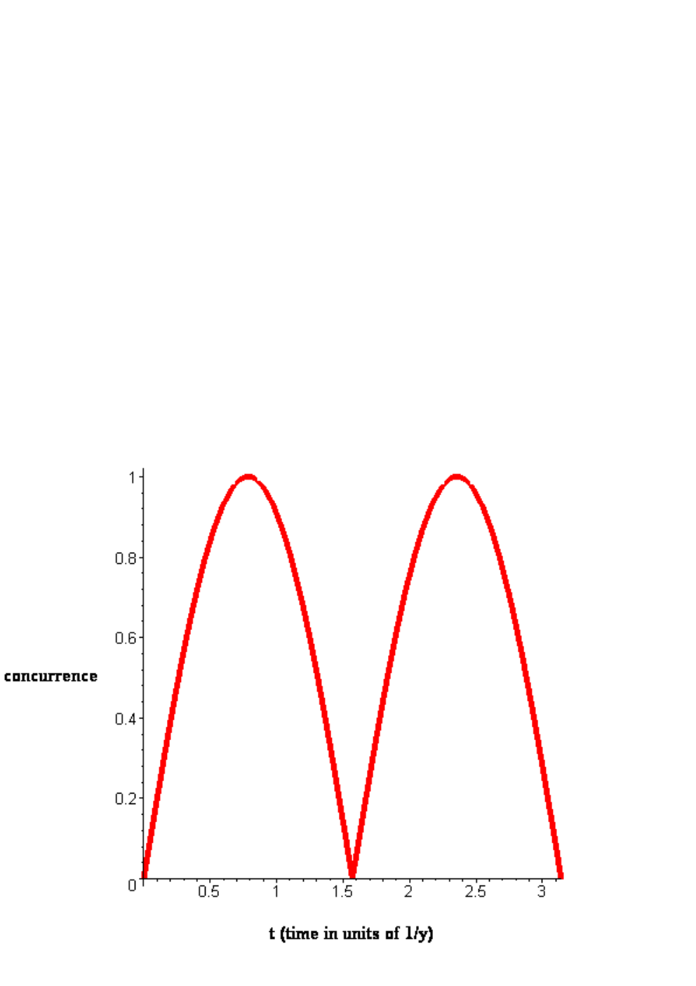
The off-diagonal coupling term changes the entanglement. This can be used to create entanglement but it also destroys entanglement.
Referring to Figure 1, we see immediately that if we start in the state then at (in units of ) we have the maximally entangled (Bell) state (up to a global phase factor) but the unitary action destroys the entanglement, completely at .
3. Environmental Dissipation
The standard form of a general Markovian dissipative process in Quantum Mechanics is governed by the Liouville equation obtained by adding a dissipation (super-)operator to the usual hamiltonian term:
| (3.1) |
where the density matrix for an -level system is an (semi-)positive matrix.
3.1. Lindblad Equation
In order that the quantum Liouville equation Eq.(3.1) should define a physical dissipation process, certain constraints must be imposed, most notably complete positivity. The appropriate constraints emerge from physical stochastic dissipation equations such as those given by Lindblad and others in differential form [4], as well as in global form [5]. The result is that completely positive evolution of the system is guaranteed provided the dissipation super-operator takes following form
| (3.2) |
where the matrices are arbitrary. Denoting the standard basis for matrices by
| (3.3) |
and relabelling, using the notation , we have
| (3.4) |
The virtue of Eq. (3.1) is that every Markovian dissipation process has to satisfy it and so results derived from its use have great generality. A drawback, however, is that it is often not obvious how to relate phenomenological observations of dissipative effects to dissipation operators of the form (3.2).
3.2. Phenomenological description
Having chosen a certain computational or preferred basis, one can phenomenologically distinguish two types of dissipation: phase decoherence and population relaxation. The former occurs when the interaction with the environment destroys the phase correlations of certain superposition states. In the simplest case this leads to a decay of the diagonal elements of the density operator at a constant (dephasing) rate :
| (3.5) |
Population relaxation occurs, for instance, when a quantum particle in a certain state spontaneously emits a photon and transitions to a less energetic quantum state. In the simplest case, when there are only jumps between the basis states, and say, occurring at fixed rates , the resulting population changes can be modelled as
| (3.6) |
where is the population loss for level due to transitions , and is the population gain caused by transitions . The population relaxation rate is determined by the lifetime of the state and, for multiple decay pathways, the relative probability for the transition .
Phase decoherence and population relaxation lead to a dissipation super-operator (represented by an matrix) whose non-zero elements are
| (3.7a) | |||||
| (3.7b) | |||||
| (3.7c) | |||||
where and are taken to be positive numbers, with symmetric in its indices, and again we employ the convenient notation introduce above.
The matrix super-operator may be thought of as acting on the -vector obtained from by
| (3.8) |
The resulting vector equation is
| (3.9) |
where is the anti-hermitian matrix corresponding to the hamiltonian . We obtain explicitly by using the standard algebraic trick applied in evaluating Liouville equations (see, for example [2]). The correspondence between and as given in Eq. (3.8) tells us, after some manipulation of indices, that
| (3.10) |
using the direct (Kronecker) product of matrices.
3.3. Constraints on Dephasing Rates
The phenomenological description above does not impose any constraints on the population relaxation and decoherence parameters present in the dissipation matrix. In practice, however, the values of the dissipation parameters and must satisfy various constraints [3] to ensure that they describe physical processes, which can be derived by use of the Lindblad equation.
For simplicity we restrict ourselves here to the case of pure dephasing. Experimentally, this is often the dominant decoherence process as the population relaxation (or ) times for most systems are much longer than the dephasing (or ) times so that we may effectively neglect the relaxation rates . In the pure decoherence (dephasing) case, comparison of Eq.(3.2) and Eq.(3.4) with Eq.(3.7) tells us that the terms vanish if we choose for . The decoherence parameters are then given by
| (3.11) |
This leads to a mathematically very simple situation, as the dissipation matrix is then diagonal. For the system, this gives six pure dephasing parameters (, ), determined by four constants, so there are two relations between the ’s. Explicitly, we have for the two-qubit, 4-level case,
| (3.12a) | ||||
with , and the constraints that must be imposed to ensure that we have physical process are then
| (3.13) |
3.4. Markovian dissipation of entanglement
We now give an example of a standard dephasing process acting on a maximally entangled state.
Example 1.
Consider the Bell state
| (3.14) |
The corresponding Liouville vector is and the action of the dephasing operator of Eq.(3.12) is given by
| (3.15) |
as in Eq. (3.9). This equation may be immediately integrated to give
| (3.16) |
corresponding to the density matrix
| (3.17) |
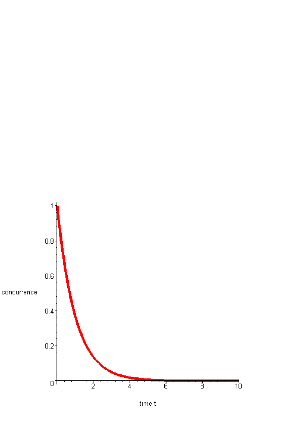
Note that this does not represent a pure state except at . The concurrence as defined in Section 2.1 evaluates to . (See Figure 2).
4. Quantum control of entanglement dissipation
In this section we analyze two quantum control schemes for mitigating entanglement dissipation. We first consider a simple scheme based on open-loop coherent control and then a measurement-based feedback scheme.
4.1. Coherent quantum control
For pure dephasing and a hamiltonian of the form (2.1) the -subspace is invariant, i.e. if a state starts in this subspace it remains there. Thus if the system is initially prepared in the Bell state Eq. (3.14) then we may consider the reduced dynamics on the -subspace. The density operator restricted to the -subspace is essentially a qubit, i.e., a positive matrix . Introducing the Pauli matrices
| (4.1) |
then the Lindblad equation Eq(3.2), with a single term , takes the simple form
| (4.2) |
where .
It is convenient to use the Bloch representation, for which the 3-vector associated with the density matrix is given by
| (4.3) |
For hamiltonian dynamics, is constant and the motion is governed by the orthogonal group acting on the Bloch Sphere. In the case of dissipation, the motion takes place in its interior, the Bloch Ball, and is locally governed by the affine Lie algebra ; this is globally a semi-group due to boundary conditions [7]. Therefore in general the Bloch equation is
| (4.4) |
In the simple case considered here, we have
| (4.5) |
For the Bloch matrix is invertible and any initial state eventually goes to the unique steady state , which corresponds to the completely mixed state on the -subspace, which has zero concurrence. Thus regardless of the value of the control the system will eventually go to the completely mixed state on the -subspace and all entanglement will be lost. If (no control) then all the Bloch vectors along the -axis in the -subspace are steady states, but if we start with a Bell state we still go to the completely mixed state on the subspace for . So in this case there is no way coherent control can prevent the decay of the entanglement. This is understandable as the hamiltonian term determines the anti-symmetric part of while the decoherence term defines the symmetric part, so the control cannot change the contraction of the Bloch vector introduced by the dephasing term. If we want to stabilize an entangled state we need to employ a more sophisticated method. One approach is to utilize a measurement and feedback scheme.
4.2. Measurement/feedback control scheme
One approach that has shown recent promise in particular for stabilizing quantum states [8] is reservoir engineering, in particular using direct feedback.
Suppose we have a system whose evolution is governed by a Lindblad master equation (3.1). If we add a fixed continuous weak measurement of an observable and apply a fixed feedback hamiltonian conditioned directly on the measurement current, then according to the general theory developed by Wiseman and Milburn [9, 10] the master equation is modified as follows:
| (4.6) |
where is the original system hamiltonian plus the open-loop control hamiltonian plus a feedback correction term (see the diagrammatic scheme of Figure 3).
Suppose we have a system with hamiltonian as in (2.1) subject to environmental dephasing described by a diagonal Lindblad operator . If we now add a weak continuous measurement of the observable and apply a feedback hamiltonian of the form then the evolution of the system according to (4.6) is governed by
| (4.7) |
As observed before, the subspace is invariant under and . It is also invariant under , i.e. any state starting in this subspace will remain in it. Thus, if we are only interested in initial states in this subspace we can again restrict our attention to the dynamics on this subspace. The subspace operators are
| (4.8) |
and noting that shows that the master equation for the density operator restricted to the subspace takes the form
| (4.9) |
Here is the effective energy level splitting and the effective environmental decoherence rate, and , and are the effective strengths of the open-loop control, measurement and feedback, respectively. The corresponding Bloch operator is
| (4.10) |
and .
For calculational simplicity we choose the open-loop control term to be , i.e., . In this case it is easy to compute the eigenvalues of :
| (4.11) |
Thus is non-degenerate if and the system therefore has a unique steady state on the subspace, which in density operator form is
| (4.12) |
The purity of the steady state is given by
| (4.13) |
and the concurrence is
| (4.14) |
Note that , i.e. there is a one-to-one correspondence between the concurrence and purity in this case. If we further choose (adjust energy level splitting to be ) then the expressions simplify:
| (4.15) |
and the purity and concurrence are given by
| (4.16) | ||||
| (4.17) |
For a given fixed decoherence rate , we can choose and in units of and set . In this case the steady-state concurrence becomes
| (4.18) |
Figure 4 shows the logarithm of as a function of the measurement and feedback strengths. We see that the optimum choice to maximize the concurrence is with and as large as practically feasible. The plot given in Figure 4 shows that if the measurement and feedback strengths are about 100 times the environmental decoherence rate then the steady-state concurrence is greater than .
Although this scheme may be difficult to realize in practice because we require a non-local feedback hamiltonian of the form , with some experimental ingenuity such a procedure may well be implemented.
References
- [1] Wootters W K 1998 Phys. Rev. Lett. 80, 2245-2248
- [2] Havel T F 2003 J. Math. Phys. 44, 534
- [3] Schirmer S G and Solomon A I 2004 Phys. Rev. A 70, 022107
- [4]
Lindblad G 1976 Comm. Math. Phys. 48, 119
Lindblad G 1975 Comm. Math. Phys. 40, 147
Gorini V, Kossakowski A, and Sudarshan E C G 1976 J. Math. Phys. 17, 821 - [5]
Sudarshan E C G, Matthews P M, and Rau J 1961 Phys. Rev.121, 920
Kraus K 1971 Ann.Phys.64 311 - [6] Solomon A I 2008 European Physical Journal (Special Topics) 160 391
- [7] Solomon A I and Schirmer S G 2002 Dissipative ‘Groups’ and the Bloch Ball CONFERENCE SERIES- INSTITUTE OF PHYSICS 173 485
- [8] S. G. Schirmer, X. Wang, Phys. Rev. A 81, 062306 (2010); Ticozzi, S. G. Schirmer, X. Wang, IEEE Trans. Autom. Control (2010)
- [9] Wiseman H M 1994 Phys. Rev. A 49, 2133
- [10] Wiseman H M and Milburn G J 2010 Quantum Measurement and Control Cambridge: CUP). See especially Chapter 5.
.