Quadrupole moment of a magnetically confined mountain on an accreting neutron star: effect of the equation of state
Abstract
Magnetically confined mountains on accreting neutron stars are promising sources of continuous-wave gravitational radiation and are currently the targets of directed searches with long-baseline detectors like the Laser Interferometer Gravitational Wave Observatory (LIGO). In this paper, previous ideal-magnetohydrodynamic models of isothermal mountains are generalized to a range of physically motivated, adiabatic equations of state. It is found that the mass ellipticity drops substantially, from (isothermal) to (non-relativistic degenerate neutrons), (relativistic degenerate electrons) and (non-relativistic degenerate electrons) (assuming a magnetic field of at birth). The characteristic mass at which the magnetic dipole moment halves from its initial value is also modified, from (isothermal) to , , and for the above three equations of state, respectively. Similar results are obtained for a realistic, piecewise-polytropic nuclear equation of state. The adiabatic models are consistent with current LIGO upper limits, unlike the isothermal models. Updated estimates of gravitational-wave detectability are made. Monte Carlo simulations of the spin distribution of accreting millisecond pulsars including gravitational-wave stalling agree better with observations for certain adiabatic equations of state, implying that X-ray spin measurements can probe the equation of state when coupled with magnetic mountain models.
Keywords:
accretion, accretion discs – stars: magnetic field – stars: neutron – pulsars: general1 Introduction
Neutron star spins in low-mass X-ray binaries (LMXBs), measured from X-ray pulsations or thermonuclear burst oscillations, are found to lie in the range (Chakrabarty 2008; Galloway 2008; Watts et al. 2008; Galloway et al. 2010). The upper end of this range falls well short of the centrifugal breakup frequency for most equations of state (Cook et al. 1994; Haensel et al. 1999; Chakrabarty 2008), even though the objects accrete enough angular momentum during their X-ray lifetime of years (Podsiadlowski et al. 2002) to spin up to (Bildsten 1998; Chakrabarty et al. 2003). This discrepancy cannot be attributed to an observational selection effect, because the Rossi X-ray Timing Explorer (RXTE) remains sensitive up to (Chakrabarty 2008; Galloway 2008). To describe the apparent spin clustering and cut-off, Bildsten (1998) invoked gravitational radiation torques to stall the spin-up process; see also Papaloizou & Pringle (1978) and Wagoner (1984). To achieve this, a mass quadrupole moment of order is required.
Quadrupoles on accreting neutron stars are of two kinds: (i) core deformations, e.g. from r-modes (Brink et al. 2004; Nayyar & Owen 2006; Bondarescu et al. 2007) and (ii) permanent crustal deformations, e.g. supported by thermal (Bildsten 1998; Ushomirsky et al. 2000) or magnetic (Brown & Bildsten 1998; Melatos & Phinney 2001; Choudhuri & Konar 2002; Payne & Melatos 2004; Vigelius & Melatos 2008) gradients. In the absence of a magnetic field, the maximum crustal quadrupole depends on the breaking strain (Ushomirsky et al. 2000; Haskell et al. 2006) and can be as large as in the light of recent molecular dynamics simulations (Horowitz & Kadau 2009). When magnetic stresses are included, the quadrupole increases, as matter is funnelled to the magnetic poles of the star and compresses the magnetic field laterally (Hameury et al. 1983; Melatos & Phinney 2001; Choudhuri & Konar 2002; Payne & Melatos 2004; Vigelius & Melatos 2008).
Payne & Melatos (2004), hereafter PM04, calculated self-consistent, axisymmetric, ideal-magnetohydrodynamic (ideal-MHD) equilibria of isothermal magnetic mountains as a function of accreted mass . They found that the magnetic field distorts appreciably for , in accord with the phenomenological field decay relation of Shibazaki et al. (1989) and well above previous calculations, which predicted without including the back reaction from the compressed equatorial magnetic field (Hameury et al. 1983; Brown & Bildsten 1998; Litwin et al. 2001). Payne & Melatos (2007) showed that the mountain oscillates stably in a superposition of Alfvén and acoustic modes when perturbed, following a transient adjustment via the undular submode of the magnetic buoyancy instability (Mouschovias 1974; Hughes & Cattaneo 1987; Vigelius & Melatos 2008). Vigelius & Melatos (2008) found that the equilibrium state remains mountain-like after this transient instability, with the mass quadrupole moment decreasing by per cent. Ohmic dissipation contributes to the decay of the mass quadrupole by allowing slippage of accreted matter across magnetic field lines, with a resistive relaxation timescale of depending on the conductivity (Vigelius & Melatos 2009b). Wette et al. (2010) examined the subsidence of mountains into a fluid crust, generalizing earlier calculations on a rigid surface, and found that the quadrupole shrinks by up to per cent.
The existing literature on magnetic mountains, summarized above, suffers from several limitations. First, the time-dependent feedback between the magnetosphere and the accretion disc is neglected (Romanova et al. 2003; Romanova et al. 2004; Kulkarni & Romanova 2008; Long et al. 2008). Secondly, the mountain should solidify into a body-centred-cubic crystal as it sinks, when the ionic coupling parameter exceeds the crystallization threshold (Farouki & Hamaguchi 1993; Horowitz & Berry 2009). This occurs at different depths, depending on the local composition, density and temperature (Brown 2000). The sudden transition to a solid affects the magnetic line-tying boundary condition, which now depends on the local magnetic stresses and critical strain. Thirdly, a nuclear reaction network that follows accreted matter elements as they descend has not yet been implemented (Haensel & Zdunik 1990a; Haensel & Zdunik 1990b; Haensel & Zdunik 2003; Chamel & Haensel 2008). Deep crustal heating deposits per accreted baryon (Haensel & Zdunik 2008), reduces the Ohmic decay time-scale, and introduces thermal and electrical conductivity gradients due to compositional variations (Chamel & Haensel 2008), all of which affect the mountain structure. Finally, the equation of state (EOS) of the accreted matter needs to be modelled realistically. The calculations cited in the previous paragraph all utilize an isothermal EOS, an accurate model for very low mass mountains with maximum density (Shapiro & Teukolsky 1983). The isothermal EOS is too soft and does not accurately represent all pressure components (e.g. degenerate neutron and electron pressures in the inner crust) for realistically sized mountains with or equivalently (Shapiro & Teukolsky 1983; Brown 2000; Chamel & Haensel 2008).
This work aims to quantify how the EOS influences the structure of the magnetic mountain and its mass quadrupole moment. It turns out that the effect is large. In Section 2, we generalize the Grad–Shafranov framework for solving numerically the MHD equilibrium problem to incorporate an adiabatic EOS. The numerical algorithm is validated against published isothermal results in Section 3. We directly compare the structure of adiabatic and isothermal magnetic mountains in Section 4, quantifying the relation between the accreted mass and measurable quantities such as dipole moment and ellipticity. In Section 5, we approximate the realistic EOS in the neutron star crust by an effective polytrope and calculate the structure of the associated mountain. In Section 6, we examine the implications of the theoretical models for gravitational-wave (GW) stalling of LMXB spins. The detectability of magnetic mountains as GW sources is assessed briefly in Section 7, revising the latest estimates in Vigelius & Melatos (2009a).
2 Hydromagnetic Equilibrium
To compute the structure of a magnetic mountain with an adiabatic EOS, we generalize the isothermal Grad–Shafranov solver described in PM04 to handle a general, barotropic, pressure-density relation of the form , where is the polytropic index and is the adiabatic index (Paczynski 1983; Shapiro & Teukolsky 1983).
2.1 Grad–Shafranov equation
Let us define a spherical coordinate system , where is the magnetic symmetry axis before accretion begins and the neutron star surface is situated at (i.e. the inner boundary of the simulation; see Appendix A). Time-dependent ideal MHD and resistive simulations of magnetic mountains in ZEUS-MP show that the magnetic field relaxes to an almost axisymmetric configuration (deviation from axisymmetry per cent) within a few Alfvén times, following a transient, Parker-type instability (Vigelius & Melatos 2008). Hence, to a good approximation, the magnetic field is given everywhere by
| (1) |
where is a flux function. In the steady state, the MHD equations reduce to
| (2) |
where denotes the Grad–Shafranov operator,
| (3) |
We solve the projection of equation (2) along by the method of characteristics. The result depends critically on the EOS. Under isothermal conditions, i.e. , we find
| (4) |
where denotes the reference gravitational potential at the neutron star surface, and is the isothermal sound speed (Payne & Melatos 2004). Under adiabatic conditions, i.e. , we find
| (5) |
The pressure along a flux surface under isothermal and adiabatic conditions is given by
| (6) |
and
| (7) |
respectively. Formally speaking, is an arbitrary function of the magnetic flux in equations (4)–(7). Equation (6) is the usual barometric formula; the base pressure varies from field line to field line, and decreases with arc length along any particular field line because is inversely proportional to . Equation (7) behaves similarly, but its form is not barometric, in the sense that does not factorize out.
In order to establish a one-to-one mapping between the initial (pre-accretion) and final (post-accretion) states that preserves the flux freezing encoded in the mass-continuity and magnetic-induction equations of ideal MHD, we require that the final, steady-state, mass-flux distribution , defined as the mass enclosed by the infinitesimally separated flux surfaces and , equals that of the initial state plus the accreted mass. This approach uniquely determines through
| (8) |
for the isothermal EOS and
| (9) | ||||
for the adiabatic EOS. This approach is self-consistent and therefore preferable to guessing (Hameury et al. 1983; Brown & Bildsten 1998; Melatos & Phinney 2001), but it renders the solution more difficult. [Duez & Mathis (2010) also solved self-consistently for by minimizing the total energy while conserving invariants like the helicity and mass-flux ratio.] The integrals in equations (8) and (9) are performed along the magnetic field line . In accordance with earlier work, we prescribe the mass-flux distribution in one hemisphere to be
| (10) |
where is the accreted mass, labels the flux surface emerging from the magnetic equator, labels the field line that closes just inside the inner edge of the accretion disc, and we write . Equation (10) ensures that per cent of the accreted mass accumulates within the polar cap for .
The gravitational acceleration is assumed to be constant in this paper, with a gravitational potential of the form . This assumption is justified, because the mountain never rises more than above the hard surface at (see Section 4.5). A simple numerical check shows that the altitude above where the density distribution falls to zero changes by per cent when is replaced by . Self-gravity is also ignored, although the correction to the gravitational potential is significant in LMXBs with .
We conduct our numerical simulations as follows: a fixed dipolar magnetic field at the inner radial boundary of the numerical mesh is assumed, and a prescribed amount of accreted matter (described by one of the EOS in Table 1) is added into the simulation volume according to the mass-flux relation (10). We then allow the system to relax quasi-statically to hydromagnetic equilibrium by solving equation (4) or (5) simultaneously with equation (8) or (9) for , using an iterative under-relaxation algorithm combined with a finite-difference Poisson solver. The details can be found in Appendix A. We adopt the following boundary conditions, as in previous papers (e.g. PM04): (surface dipole; magnetic line tying), (outflow), (straight polar field line) and (north–south symmetry), where and delimit the computational volume. The outer radius is chosen large enough to encompass most of the screening currents (isothermal EOS) or the outer edge of the accreted matter (adiabatic EOS).
2.2 Inner boundary
The nature of the rigid inner boundary at deserves special mention. It is not the stellar surface; it is not meaningful to build a mountain high and reaching neutron drip density at its base on top of a low-density ocean, using a realistic EOS. Instead, the outer layers of the neutron star are ‘constructed’ from the accreted material of mass . Thus, does not correspond to the neutron star surface , but to the depth in the neutron star crust above which lies the mass (for a given EOS). Since and are fixed, the total mass and radius vary slightly (few per cent) between models with different but the same EOS (Table 1). The inner boundary of our simulation volume represents a solid surface at the corresponding base density. This simplification assumes that movement of matter below this depth is approximately radial due to compression and that the solid-surface prescription is valid. In reality, accreting matter is expected to displace both radially and laterally (Choudhuri & Konar 2002). The lateral flow would alter our computed results by decreasing the mass quadrupole moment slightly and increasing the magnetic dipole moment. We can eliminate this approximation by injecting the accreted matter according to the approach advocated by Wette et al. (2010), generalizing the latter paper to a realistic EOS. Such a procedure is feasible but technically difficult; we defer it to future work.
Referring to fig. 12 of Wette et al. (2010), the ellipticity of an isothermal mountain in the fluid-surface model appears to converge to the saturation ellipticity of the hard-surface model as increases; the difference in ellipticities relative to the hard-surface model decreases from to per cent as increases from to . We expect similar convergent behaviour for adiabatic mountains at significantly lower , since saturation ellipticities of adiabatic mountains are attained at accreted masses – orders of magnitude below that of the isothermal one (see Fig. 4). Realistic accreted masses in LMXB systems of are – orders of magnitude greater (depending on the EOS) than the accreted masses which we can reliably simulate. At realistic accreted masses, we expect the saturation ellipticities of mountains with and without sinking to approximately converge. The population-synthesis results in Section 6 and GW-detectability estimates in Section 7 depend solely on the saturation ellipticity.
2.3 Adiabatic index
The realistic EOS of a neutron star crust is piecewise adiabatic, as discussed in Section 5. However, before modelling the realistic EOS, we conduct numerical experiments in Sections 3 and 4 to see how the mountain structure depends on the adiabatic index . In these numerical experiments, we employ a purely adiabatic EOS with unique and . The values of and are chosen to correspond to density regimes of interest in the crust, e.g. degenerate non-relativistic electron gas , degenerate relativistic electron gas and degenerate neutron gas . In an ideal electron gas, which is approximately isothermal, radiation and lattice pressures dominate, but this occurs at much lower densities , which are irrelevant to the mountain problem.
Table 1 displays the magnetic mountain models we compute here, with the details of their respective EOS. is a function of mean molecular weight per electron, , according to the scaling , where is the mean baryon rest mass, is the atomic mass unit, and is the mean number of electrons per baryon. Under the assumption of symmetric nuclear matter, we take and and hence is a constant (i.e. independent of ). This form of the EOS describes well a completely degenerate, ideal Fermi gas (Shapiro & Teukolsky 1983). Hence we use it to model degenerate relativistic electrons (), degenerate non-relativistic electrons () and degenerate non-relativistic neutrons ().
| Model | (cgs) | Equation of State | |
|---|---|---|---|
| A | 1 | Isothermal | |
| B | 5/3 | Non-relativistic degenerate electrons | |
| C | 4/3 | Relativistic degenerate electrons | |
| D | 5/3 | Non-relativistic degenerate neutrons | |
| E | Variable | Variable | Piecewise polytropic |
3 Validation in the isothermal limit
We assume the following neutron star parameters throughout this paper, except where stipulated otherwise: , and (with , where is the polar magnetic field strength before accretion begins). The fiducial value of the magnetic field, , is chosen in accord with population synthesis models, which predict natal magnetic fields of (Hartman et al. 1997; Arzoumanian et al. 2002; Faucher-Giguère & Kaspi 2006).
The adiabatic Grad–Shafranov formalism in Section 2, and the numerical solver described in Appendix A, must reproduce the results of PM04 in the isothermal limit (i.e. ). In this limit, the isodensity contours and magnetic field lines of an adiabatic mountain with must converge to those plotted in figs 4, 5 and 9 in PM04 for identical accreted masses. As there is no unique way to continuously transform an adiabatic EOS into an isothermal EOS, we test the adiabatic/isothermal correspondence by taking the limit in three different ways below.
- 1.
We set and let tend to unity, such that
(11) - 2.
Exploiting the tendency for the surface pressure and density to be roughly EOS-independent for , we write to eliminate , and hence obtain
(12) where is a function of .
- 3.
We take and interpolate between a selected polytrope and the isothermal target according to
(13) with .
We apply these three approaches to the case , starting from a relativistic degenerate electron EOS (model C in Table 1). This EOS prevails over a large logarithmic range of densities in a realistic stellar crust [; see Section 5] and gives way to an isothermal EOS in the upper atmosphere (). We find that all three approaches converge correctly to the results of PM04 after iterations. Fig. 1 displays the mass ellipticity, magnetic dipole moment, and grid-averaged residual (relative to the result) as a function of for approaches (i) (red diamonds), (ii) (green rectangles) and (iii) (blue triangles). As indicated by Fig. 1, the rate of convergence towards the isothermal results differs between models. The abnormally high dipole moment for case (i) at in Fig. 1 is caused by insufficient resolution in and can be prevented by scaling the grid logarithmically in to handle the steep magnetic field gradients at the equator. We defer this project to future work.
We compute the mass enclosed within the computational grid as a function of iteration number, to track the mass lost through the outer boundary. In every converged equilibrium, the total mass in the final state is always within per cent (and typically within per cent) of the initial mass. The iterative solver also preserves the divergence-free nature of the magnetic field, with to machine precision everywhere on the grid.


4 Adiabatic mountains
In this section, we compute Grad–Shafranov equilibria for several adiabatic EOS using the method described in Section 2 and validated in Section 3. Table 1 lists the parameters of each EOS, corresponding to different depth intervals within the stellar crust (see Section 5). The scalings of the magnetic dipole moment and mass ellipticity with accreted mass are studied in Sections 4.1 and 4.2, respectively. The maximum density and local magnetic field strength are computed in Sections 4.3 and 4.4, respectively. In Section 4.5, we compare the equilibrium density and magnetic field distributions for adiabatic and isothermal magnetic mountains. For each model in Table 1, we stop our simulations once is less than per cent averaged over the grid (see Appendix A).
4.1 Magnetic burial: versus
As accretion proceeds and the initial dipolar magnetic field lines are distorted, magnetic energy is transferred from the dipole to higher order multipole moments. The north–south antisymmetry of precludes the existence of even multipoles. Fig. 2 displays the magnetic dipole moment (normalized by its initial, or surface, value) as a function of the accreted mass for models A–E in Table 1. The maximum accreted mass for which the iterative solver converges reliably (grid-averaged residual per cent) depends on the EOS, with for models A–D, respectively. (As a corollary, the gradient in the vicinity of the rightmost data point for each model in Fig. 2 is unphysically steep.) The method we use to calculate the dipole moment differs slightly from that in PM04; we integrate directly rather than , according to
| (14) |
for the lth multipole moment, circumventing one set of numerical derivatives and improving the accuracy of the results. Equation (14) is per cent more accurate than equation (34) in PM04 for a grid. The discrepancy shrinks to per cent for a grid.
It is clear from Fig. 2 that the characteristic mass required to significantly distort the initial configuration varies with the EOS. If we define to be the accreted mass that halves from its initial value , to be consistent with the empirical scaling introduced by Shibazaki et al. (1989), viz.
| (15) |
then Fig. 2 yields , , and for models A–D in Table 1. Plainly, varying the EOS makes a big difference. is reduced by a factor of between (model D) and (model B) relative to an isothermal mountain. This is because adiabatic mountains are up to times taller than isothermal ones for (see Fig. 3 below and Section 4.5). At higher altitudes, the magnetic stress () is weaker and hence the pressure gradient pushes the magnetic field sideways more than in an isothermal mountain.
In the limit of small , one can show (see Appendix B) that the scaling of the characteristic mass for adiabatic mountains is proportional to the square of the magnetic field strength, as for isothermal magnetic mountains (see Section 3.2 in PM04). Additionally, is also inversely proportional to an extra factor (evaluated as a contour plot on the – plane in Fig. 14), which depends only on the EOS parameters and the accreted mass through equations (41) and (45). In this limit, one finds the following scalings of the magnetic dipole moment: (model A), (models B and D) and (model C), where are constants. We confirm in Section 5 that the realistic EOS (model E) is well approximated by model C and hence follows the same scaling. It is important to note that these scalings are only valid in the small- limit (i.e. , where is EOS-dependent). For , the analytical solution no longer applies and numerical results have to be used.
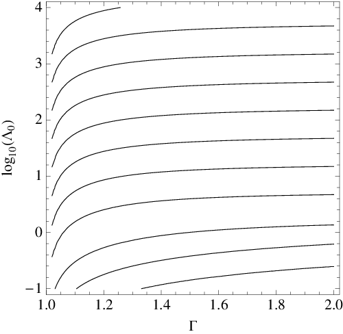
In Fig. 3, we plot as a function of altitude above the surface for models A–D by replacing with in equation (14). The purpose is to illustrate how the screening currents are distributed radially for different EOS. The accreted masses are chosen to be the characteristic masses of each model in Table 1. The dipole moment turns up by per cent at because the Neumann boundary condition , which holds the field lines perpendicular to the outer grid boundary, does not apply strictly to a dipole field. For the isothermal mountain (model A), the screening currents are located times closer to the neutron star surface than in models B–D, and the isodensity contours contract towards the surface by the same factor (see Section 4.5).


4.2 Mass quadrupole: versus
Fig. 4 displays the mass quadrupole moment of the mountain, expressed in terms of the mass ellipticity , as a function of . The ellipticity is given by , where denotes the moment-of-inertia tensor, the -axis lies along the magnetic axis of symmetry, and we define . To zeroth order, both and are proportional to the surface density . Hence, the ellipticity is proportional to accreted mass for . At , the hydrostatic pressure overwhelms the Lorentz force and the mountain spreads laterally, distributing the extra accreted mass evenly over a larger area (the enlarged magnetic polar cap) and moderating the growth of the ellipticity such that .
The apparent turnover in after it peaks in Fig. 4 is a numerical artefact, which sets in as the convergence of the numerical algorithm worsens (see Section 4.1). In reality, for , the ellipticity saturates at the value where in a hard-surface model. Wette et al. (2010) examined accretion on to a non-rigid neutron star crust, thereby allowing the accreted matter to sink, and showed that the ellipticity does not saturate (i.e. ) up to . Despite this monotonic increase, the ellipticity of soft-surface mountains is always less than that of hard-surface mountains by – per cent in the mass range .

4.3 Equatorial magnetic compression


The accreted matter transports frozen-in magnetic flux equatorward as it spreads sideways under its own weight. As a result, the magnetic field lines are ‘pinched’ near the surface at the equator and flare outwards at higher altitudes like a ‘tutu’ (Melatos & Phinney 2001; Payne & Melatos 2006). The maximum magnetic field strength in the equatorial belt is computed as a function of and graphed in Fig. 5 for models A–D in Table 1. Naturally, the latitude where maximizes moves towards the equator as increases, and the equatorial belt narrows. From Fig. 5, we see that adiabatic magnetic mountains produce a larger (and hence a narrower belt, by flux conservation) than isothermal ones with the same . Referring to Fig. 6, this can be understood as follows. The top panel of Fig. 6 shows the equilibrium magnetic field configuration of an adiabatic and an isothermal mountain, at their characteristic masses (these masses are different since is EOS-dependent). At equilibrium, the hydrostatic pressure gradient at the base of the mountain (dotted red/blue arrow for adiabatic/isothermal mountain in Fig. 6) is balanced by magnetic stresses (red/blue arrow for adiabatic/isothermal mountain in Fig. 6) within the equatorial magnetic belt (the extent of the magnetic belt is denoted by red/blue shaded regions for adiabatic/isothermal mountains in Fig. 6). The hydrostatic pressure gradients for both EOSs are comparable at characteristic accreted masses, because the magnetic field lines are bent by a similar angle for all models at [since is EOS-independent]. This can be expressed equivalently in terms of the comparable width of the equatorial magnetic belt of both mountains, since comparable deformation angles of the magnetic field lines result in corresponding widths of the magnetic belt. Referring to the bottom panel of Fig. 6, the hydrostatic pressure gradient at the base of the accreted layer is greater for adiabatic mountains than isothermal ones at an equivalent , because , where the subscripts A–D denote the models in Table 1 (see Section 4.1). Hence, magnetic-field lines of an adiabatic mountain are more deformed than those of an isothermal one to counteract this. This decreases the lateral extent of the magnetic belt and, by magnetic flux conservation, increases as the belt shrinks. This explains why the point where is reached moves equatorward as increases, and why is greater for an adiabatic rather than an isothermal mountain for the same .
The compressed magnetic field can surpass the yield strength of the crust, at which point the magnetic stresses break the Coulomb lattice as the field deforms. Taking the breaking strain of the neutron star crust to be from recent molecular dynamics simulations (Horowitz & Kadau 2009), the magnetic field strength at which the crustal matter yields (Romani 1990) is
| (16) |
where and are the mean atomic and mass numbers, respectively. We evaluate at the base of a mountain of mass from the nuclides present at base pressure (Haensel & Zdunik 1990a; Haensel & Zdunik 1990b; Chamel & Haensel 2008). The results are plotted as curves in Fig. 5 for the models in Table 1. In an isothermal mountain, we find , so that the accreted matter does not crack and remains polycrystalline, with a frozen-in magnetic field. As the substrate of an isothermal mountain does not spread significantly, and are larger. Indeed, strictly speaking, crustal freezing should be included in the boundary conditions of an isothermal mountain calculation (implemented dynamically at the depth where it first occurs). On the other hand, adiabatic mountains compress the magnetic field in excess of for and for models D and C respectively, while is surpassed for all accreted masses in the case of model B. This suggests that the accreted matter continuously cracks or flows plastically at most depths (Horowitz & Kadau 2009), validating the fluid approximation for models with .
4.4 Maximum Density
The maximum density at the base of a magnetic mountain is reached at the magnetic pole (see Section 4.5). We extract the maximum density as a function of from the simulated models listed in Table 1 and graph the results in Fig. 7.
A deficiency of isothermal mountains, noted by PM04, is the unrealistically high density at the base, which exceeds the neutron drip point11 1 depends on whether the crust is cold-catalyzed or accreted, as well as the exact EOS (Chamel & Haensel 2008). Here we consider the compressible liquid drop model for the EOS of the accreted crust (Haensel & Zdunik 1990a; Haensel & Zdunik 1990b; Chamel & Haensel 2008). at relatively small accreted masses of (cf. in a typical LMXB). In contrast, Fig. 7 shows that is several orders of magnitude lower for an adiabatic EOS; none of the adiabatic mountains surpass for .
At accreted masses approaching , models C and D attain crust--core densities22 2 We choose large enough to contain the crust–core transitions of both the Friedman–Pandharipande–Skyrme and Skyrme–Lyon EOS (Pethick et al. 1995; Haensel et al. 2007; Chamel & Haensel 2008). at their bases. These models are good approximations to the EOS of the neutron star crust at and , respectively (see Section 5). On the other hand, model B does not reach the crust–core interface because it is too stiff and approximates the true crustal EOS only at low densities . In the isothermal mountain (model A), exceeds for .

4.5 Hydromagnetic structure
A meridional cross-section of the magnetic mountain produced by models A–D in Table 1 is displayed in Fig. 8, for . The magnetic field lines and isodensity contours are graphed as solid and dashed curves, respectively; the shading also represents the density and is included to guide the eye. Note that the vertical scale changes dramatically from panel to panel. Adiabatic mountains stand times higher than an isothermal mountain for (see also Section 4.1). Moreover, one finds as in an isothermal mountain, whereas an adiabatic mountain drops to at a finite altitude. Mountains with an ideal degenerate electron gas EOS (models B and C in Table 1) are approximately 1 order of magnitude taller than those with an ideal degenerate non-relativistic neutron gas EOS (model D).
The polar () and equatorial () mountain heights as well as their ratio can be estimated analytically in the small- approximation developed in Appendix B. For models B, C and D, and fiducial neutron star values (see Section 3), we obtain
| (17) |
| (18) |
| (19) |
Comparing with Fig. 8, we see that the analytic formula in Appendix B generally overestimates and underestimates . This discrepancy arises because the small- approximation assumes the magnetic field is nearly dipolar, whereas, at , the dipole is significantly deformed. For , there is better agreement between the numerical and analytical solutions.


5 Crustal equation of state
A realistic crustal EOS is not a simple polytrope. It includes various pressure contributions from thermal electrons, relativistic/non-relativistic degenerate electrons, non-relativistic degenerate neutrons and the ionic lattice (Brown 2000). These partial pressures depend on the composition of the crust; accreted matter undergoes nuclear reactions (e.g. electron captures and pycnonuclear fusion) as the mass density and electron Fermi energy of the compressed matter increases with depth (Chamel & Haensel 2008). Our models of magnetic mountains in accreting X-ray systems necessitate the inclusion of a realistic accreted EOS of the neutron star crust. In this section, we start from the realistic crustal EOS investigated by other authors (Negele & Vautherin 1973; Paczynski 1983; Brown 2000) and derive an equivalent effective adiabatic EOS () as a function of . This EOS is labelled model E in Table 1. The magnetic mountains produced by this more realistic EOS are compared with the pure adiabatic ones from Section 4.
We adopt the one-component plasma approximation for the accreted matter (Haensel & Zdunik 1990a; Haensel & Zdunik 1990b; Brown 2000; Chamel & Haensel 2008), together with the nuclear composition proposed by Haensel & Zdunik (1990a); Haensel & Zdunik (1990b) at temperature . This temperature is representative of the steady-state thermal profile for in accreting neutron stars containing no exotic matter such as a pion condensate or strange quarks in their interior (Miralda-Escude et al. 1990). The foregoing assumptions hold for accretion rates in the range .
Recent work by Read et al. (2009) [see also Vuille & Ipser (1999)] produced a four-parameter fit to the set of candidates for high-density EOSs in order to systematize the study of various observational constraints on the EOSs. The low-density EOS was assumed to be that of ground-state cold matter given by Douchin & Haensel (2001), while the high-density candidate EOSs were parametrized by three free-parameter piecewise polytropes. Since the EOS of the accreted crust is stiffer than that of a cold-catalyzed one (Chamel & Haensel 2008), making the radius of a – star – larger than that in the cold-catalyzed case (Zdunik & Haensel 2011), the effective polytropic form for the accreted crust calculated in this section can be combined with observations of accreting neutron stars to constrain the parameters of the parametric EOS of Read et al. (2009).


5.1 Partial pressures
There are three principal contributions to the pressure in a mountain at densities . They are as follows. (i) Electron pressure: this is exerted by non-relativistic, relativistic and thermal electron populations (Paczynski 1983). (ii) Lattice pressure: the ionic lattice exerts negative pressure due to electrostatic interactions within the Wigner–Seitz cells. It is calculated by fitting to the free energy in Monte Carlo simulations of a one-component plasma (Farouki & Hamaguchi 1993). (iii) Neutron pressure: the effect is included in a cold-catalyzed EOS which is parametrized to fit ground state nuclei above the neutron drip line (Negele & Vautherin 1973). We sum the partial pressures (i)–(ii) subject to pressure continuity across reaction surfaces, matching to the cold-catalyzed EOS of Negele & Vautherin (1973) at densities above neutron drip. Although the ground-state and accreted crusts contain different nuclei, their respective EOS are indistinguishable for , where the composition-insensitive neutron pressure dominates (Chamel & Haensel 2008).
The pressure and the adiabatic index of the resultant EOS are graphed versus density in Fig. 9. Although some parts of the EOS are piecewise adiabatic, other parts are not. At certain densities where electron capture reactions occur rapidly, e.g. , the density jumps discontinuously to compensate for the sharp decline in electron pressure at a compositional interface. This behaviour is accompanied by a sharp drop in the adiabatic index. These discontinuities are an artefact of the one-component plasma approximation. The presence of nuclear reactions softens the EOS for , relative to uniform composition, whereas the addition of neutron pressure stiffens the EOS for .
5.2 Effective polytrope
The realistic EOS [] in Fig. 9 is transformed into an effective adiabatic EOS, of the form , by computing the mass-weighted averages
| (20) |
for a spherically symmetric accreted layer of mass whose density profile satisfies hydrostatic equilibrium. For simplicity, we ignore general relativistic effects and assume the acceleration due to gravity to be uniform, as in models A–D.
The scaling of and with is shown in Fig. 10. The large radial variations of and within the crust imply that and depend strongly on the maximum achieved density and hence . The mass-weighted averages are dominated by the base of the mountain. Hence, the mass ellipticity and magnetic dipole moment of an adiabatic mountain with a realistic nuclear EOS depend on , not just through the weight of the accreted layer and the confining magnetic stresses but also through the density-dependent thermodynamics at the mountain’s base.
We simulate magnetic mountains with the EOS of model E for by utilizing and given in Fig. 10. The dipole moment , ellipticity , maximum magnetic field strength and maximum density of model E are compared with those of models B, C and D in Fig. 11. The hydromagnetic equilibrium for model E is also plotted in Fig. 11 for (cf. Fig. 8). As the partial pressures are dominated by relativistic degenerate electrons at , , , and in model E behave like in model C at these accreted masses. At , of model B approaches that of model C due to the presence of non-relativistic degenerate electron gas. Relativistic degenerate electrons dominate model E for , so model C can be used to approximate the realistic mountain for . For (e.g. in LMXBs), the dominant partial pressure comes from degenerate non-relativistic neutrons (model D).
For the range of natal magnetic fields inferred by Faucher-Giguère & Kaspi (2006), stays within the range where model C applies [see equations (49)–(52) of Appendix B, which give the model-dependent scaling of with respect to and ]. If rises to , appropriate for a magnetar, increases from to for model C, still below where degenerate neutron pressure dominates (see Fig. 10). We can therefore use model C to calculate under all plausible astrophysical scenarios.


6 Application to gravitational-wave spin stalling
Several mechanisms can brake the spin-up of an accreting neutron star: the magnetospheric centrifugal barrier (Illarionov & Sunyaev 1975; Ghosh & Lamb 1979), GW emission (Wagoner 1984; Bildsten 1998) and the magnetic-dipole torque (Ostriker & Gunn 1969). Every one of these mechanisms eventually balances the accretion torque and stalls the spin-up process, when the spin frequency is large enough. We use equation (21) for spin balance which assumes the usual thin-disc accretion model (Bildsten 1998). It should be noted that this is not necessarily valid, as more refined accretion models weaken the spin-up torque or strengthen the propeller effect, thus obviating the need for a strong GW torque. The feedback provided by radiation pressure in rapidly accreting systems could lead to a thick and sub-Keplerian inner accretion disc, which modulates the accretion torque of the standard thin-disc model (Andersson et al. 2005). Also, for weak accretors, if the magnetospheric radius becomes larger than the corotation radius, the star can exist in either a strong or weak ‘propeller’ phase (see Romanova et al. (2008) and references therein), with the transition between these phases being strongly dependent on the kinematic viscosity and magnetic diffusivity of the accreting matter (Romanova et al. 2004; Romanova et al. 2005). Nevertheless, these improved accretion models do not invalidate any of the proposed GW-generating mechanisms.
In this section, we investigate how the stalling frequency depends on the EOS, if all the braking comes from gravitational radiation reaction. In this work, we do not consider radiation-pressure feedback on the accretion disc since we are interested in modelling moderately accreting LMXBs where this effect is small. Also, in the vicinity of the bottom magnetic field [; see van den Heuvel & Bitzaraki (1995) and Zhang & Kojima (2006)], where the magnetosphere touches the stellar surface and the propeller effect can be neglected, the GW torque dominates the magneto-centrifugal and magnetic-dipole torques. Clearly, this approach yields an upper bound on ; the other mechanisms can lower further.
We synthesize five Monte Carlo populations of LMXBs, whose spins are such that their gravitational radiation reaction torque exactly balances the accretion torque. We assume that each simulated LMXB population undergoes magnetic burial according to one of the five EOS in Table 1. The number of neutron stars in each population is chosen large enough to yield an accurate cumulative spin distribution. We assume fiducial neutron star parameters (see Section 3) and solve
| (21) |
for the equilibrium spin frequency, assuming the wobble angle tends to due to GW back reaction (Cutler 2002) or crust–core coupling (Alpar & Saulis 1988). The accretion rates are selected from the empirical luminosity function of Galactic LMXB sources (Grimm et al. 2002),
| (22) |
where is the apparent luminosity in the band, and is the cut-off luminosity, combined with the luminosity-dependent mass fraction of the Galaxy which is visible to the RXTE All-Sky Monitor [see fig. 11 of Grimm et al. (2002)]. The long-term average bolometric luminosity is related crudely to the accretion rate by the familiar expression.
| (23) |
The results of the Monte Carlo simulations are shown in Fig. 12, where we compare the cumulative distribution function of our spin-equilibrium models with the observed distribution of nuclear-powered millisecond pulsars (NMPs) (i.e. sources that show brightness oscillations in the tails of Type I X-ray bursts), accretion-powered millisecond pulsars (AMPs) (i.e. sources that exhibit X-ray pulsations) and accreting millisecond X-ray pulsars (AMXPs) (i.e. sources that exhibit either millisecond burst oscillations, X-ray pulsations or both). We obtain data on the spins of these objects from table 1 of Watts et al. (2008). To be consistent with contemporary literature on millisecond X-ray binaries (Chakrabarty et al. 2003; Galloway 2008), we adopt the following naming convention for these sources: accreting millisecond pulsars are AMPs, burst oscillation sources are NMPs, and we combine these two populations into AMXPs33 3 By contrast, the naming convention used by Watts et al. (2008) reflects how the spins are inferred observationally: accreting millisecond pulsars, burst oscillation sources and quasi-periodic oscillation sources.. To distinguish between the confirmed and unconfirmed sources, we plot all/confirmed NMPs (thin/thick triple-dot–dashed green lines), AMPs (thick orange line) and all/confirmed AMXPs (thin/thick dashed blue lines). Curves represent cumulative distribution functions of models A (dot–dashed black curves), B (triple-dot–dashed red curves), C (short-dashed green curves), D (long-dashed blue curves) and E (solid purple curves). We update the spin of EXO 0748–676 from to (Galloway et al. 2010), and we do not discriminate between intermittent pulsars and AMPs (i.e. those sources which exhibit intermittent or persistent X-ray pulsations during outburst, respectively).
The luminosity function is defined for the RXTE All-Sky Monitor catalogue ( band), which is flux-limited below (Grimm et al. 2002). Two maximum luminosity cut-offs are investigated, namely (to include the most luminous LMXB Sco X-1) and (most luminous AMP Aql X-1), encompassing the luminosity range of all confirmed and unconfirmed AMXPs. All sources are assumed to follow the same power-law scaling of the luminosity function.
The All-Sky Monitor underestimates the true bolometric luminosity, and hence the accretion rate, due to the presence of significant hard X-ray tails in LMXB X-ray spectra (Barret 2001). Although this can be corrected (Galloway et al. 2008), we do not attempt to do so here, because equation (23) is approximate anyway, equation (21) depends weakly on , and the bolometric correction factors differ by up to per cent between sources.
Considering typical LMXB lifetimes of (Podsiadlowski et al. 2002), the accreted masses in these systems are evaluated to be in the range of . Therefore, enough matter has been transferred in these systems to reach the characteristic masses and saturation ellipticities for the models in Table 1, given initial magnetic fields of . Hence, for each simulated LMXB population, we assign the ellipticities of the neutron stars to be the saturation values for the respective EOS in Table 1.
From Fig. 12, we see that an isothermal magnetic mountain (model A) stalls the star at , where the scaling follows from of equation (30) in PM04 and equation (21). One would therefore need to fit the observed spin distribution, contradicting population synthesis studies of isolated pulsars (Hartman et al. 1997; Arzoumanian et al. 2002; Faucher-Giguère & Kaspi 2006). Adiabatic magnetic mountains (models B–E) are generally in better agreement with the observed spin distribution. In fact, models B, C and E produce a good fit to all of the observed spin distributions. Equation (49) in Appendix B for implies for models B and D, and for model C. Thus, a better fit to the empirical spin distributions can be obtained for models B and C if the fiducial magnetic field in the range of , rather than , is considered. Although model D cannot match the observed spin distribution in this range, it is possible that Ohmic diffusion can improve the agreement by allowing the mountain to spread, resulting in a lower saturation ellipticity and hence higher equilibrium spin frequencies.
It appears that the equilibrium spin frequencies of confirmed NMPs are systematically higher than those of AMPs; their cumulative distributions are offset to the right and left of the AMXP distribution, respectively (see Fig. 12). This is qualitatively consistent with the GW spin stalling mechanism, as the median time-averaged accretion luminosities of NMPs are times higher than those of AMPs, resulting in higher equilibrium spin frequencies by a factor of (under the assumption of similar ellipticities in these systems). This roughly corresponds to the frequency separation between the observed NMP and AMP distributions in Fig. 12, supporting the GW spin stalling hypothesis. On the other hand, if outburst luminosities of these objects are considered instead, the separation in predicted equilibrium spin frequencies becomes negligible.
Another noteworthy feature of Fig. 12 is the steep gradient of the observed distribution at (D. K. Galloway, private communication). The theoretical curves for models A–E can reproduce the shape of the distribution for . For the range of investigated, theoretical curves do not rise steeply enough to fit the higher-frequency () end of the distribution. This is a problem for stalling models in general, not just magnetic mountains; the scaling in equation (21) is too gentle. The observed steepening could be caused by differences between the luminosity functions of Galactic LMXB sources and AMPs/NMPs. Allowing for a realistic distribution of saturation ellipticities (e.g. due to a lognormal natal magnetic field distribution of isolated pulsars, predicted by population synthesis studies) worsens the steepening problem, if the luminosity function is assumed to be independent of the magnetic field. It is possible that another mechanism (such as the ‘propeller’ effect) sets , but its dependence on underlying variables (i.e. ) is even gentler than gravitational radiation reaction. We defer a full investigation of this puzzle to a future paper.


7 Discussion
Magnetic burial in accreting neutron stars has several important astrophysical consequences. It creates a significant mass quadrupole moment, which potentially stalls the spin-up of an LMXB by gravitational radiation reaction. It also reduces the magnetic dipole moment, in accord with the observed versus relation in neutron star binaries presented in fig. 2 in Taam & van den Heuvel (1986). In the context of the statistical evidence against field decay over in isolated pulsars (Bhattacharya et al. 1992; Lorimer et al. 1997), magnetic burial can be invoked to explain both the low magnetic fields in LMXBs and millisecond pulsars (Chanmugam 1992; Lamb & Yu 2005; Zhang & Kojima 2006) and the observed spin distribution of LMXBs (Chakrabarty et al. 2003). However, before magnetic burial is deemed a viable explanation for the above phenomena, the effect of the EOS on the burial process must be quantified.
In this paper, we show that the effect of the EOS is large. Magnetic burial is more effective for than for , in the sense that less matter must be accreted in the former case than in the latter in order to achieve the same amount of magnetic dipole screening. For the EOS listed in Table 1, decreases from (model A) to (model B), (model C), (model D) and (model E), for . Likewise, the saturation ellipticities decrease from (model A) to (model B), (model C), (model D) and (model E). This is a general result, applicable to a variety of scenarios where magnetic confinement of accreted matter can occur, such as T Tauri stars (Bertout et al. 1988; Hartmann et al. 1998), young neutron stars accreting from a fallback disc (Chatterjee et al. 2000; Wang et al. 2006) and magnetic white dwarfs (King & Lasota 1979; Wickramasinghe & Ferrario 2000). The characteristic mass scales quadratically with the magnetic field strength in all models but with different powers of the accreted mass: we have , with (model A), (model B), (model C) and (model D) (see Appendix B). The maximum density at the base of an adiabatic mountain satisfies , unlike for isothermal mountains, where it is unrealistically high. We find that crustal cracking occurs as burial proceeds, because the yield magnetic field strength is typically surpassed in non-isothermal models.
A Monte Carlo analysis of neutron stars in LMXBs, with drawn from an empirical distribution and set to the fiducial , shows that models B, C and E yield within the gravitational spin-equilibrium scenario (Bildsten 1998). This is in accord with the – confirmed spins of AMXPs. Model D predicts , slightly too low to explain the data. In comparison, the isothermal magnetic mountain (model A) does not agree with the data at all, yielding values order of magnitude lower than those from model D.
We compute the magnitude of the GW strain of the AMXPs and quasi-periodic oscillation (QPO) sources by applying the gravitational spin-equilibrium argument of Bildsten (1998) to the sources in table 1 in Watts et al. (2008). Here, we differentiate between the confirmed and unconfirmed sources, as well as AMPs, NMPs and sources that exhibit both persistent pulsations and burst oscillations. The results for AMPs (orange diamonds), confirmed NMPs (teal squares), unconfirmed NMPs (unfilled squares), QPOs (yellow triangles) and sources exhibiting both pulsations and burst oscillations (teal diamonds) are shown on a wave strain versus wave frequency plot in Fig. 13, where . The highest value considered here corresponds to , where is the maximum inferred spin in NMPs via Bayesian analysis (Chakrabarty et al. 2003). When computing , we assume that the transient sources are in torque balance during outburst. This is in accord with Hartman et al. (2008), who argued that SAX J1808.4--3658 is secularly spinning down between outbursts and is thus likely to be in spin equilibrium during outburst44 4 The transition between the spin-up and spin-down episode within the 2002 outburst of SAX J1808.4–3658 found by Burderi et al. (2006) is probably due to pulse shape changes..
The characteristic GW strain [defined in Jaranowski et al. (1998)] detectable by Laser Interferometer Gravitational Wave Observatory (LIGO) and the proposed Einstein Telescope from a periodic source at a distance of kpc [representative of Sco X-1; see Bradshaw et al. (1999)] with a false alarm rate of per cent and a false dismissal rate of per cent for a computationally feasible integration time of days is overplotted in Fig. 13 for LIGO S5 (thin solid curve), LIGO S6 (thin short-dashed curve), Advanced LIGO in the broad-band configuration (thin dot--dashed curve), lower envelope of Advanced LIGO in the narrow-band configuration (thin triple-dot--dashed curve) and the proposed conventional55 5 The xylophone configuration of the Einstein Telescope closely matches the sensitivity of the conventional configuration at frequencies (Hild et al. 2010). Einstein Telescope (thin long-dashed curve) (Hild et al. 2011; Watts et al. 2008; Smith et al. 2009). We also plot versus for neutron stars with magnetic mountains at a distance of , with magnetic field of , for models A (thick dot–dashed black curve), B (thick triple-dot–dashed red curve), C (thick short-dashed green curve), D (thick long-dashed blue curve) and E (thick solid purple curve).
Model A significantly overestimates with respect to both the interferometer sensitivity curves and the inferred Bildsten (1998) limits. In contrast, model E undercuts the Bildsten (1998) limit for QPO sources, implying either the natal magnetic fields of these sources are , or that these objects are not in GW spin equilibrium. All the confirmed AMXPs and most of the unconfirmed AMXPs are consistent with model E. They lie below the model E curve either because they have or because Ohmic diffusion prevents the ellipticity from saturating. We note that the current magnetic mountain models are still preliminary. Effects that have not yet been modelled faithfully in the context of magnetic burial may modify the saturation ellipticities. Therefore, it is still premature to quantify the absolute detectability of magnetic mountains as GW sources.
There have been two directed searches for GWs from the accreting neutron star Sco X-1 (Abbott et al. 2007a; Abbott et al. 2007b), which is expected to be the strongest emitter of its class in the GW spin stalling scenario (Bildsten 1998). The first, coherent search computed the F-statistic on 6 h of LIGO S2 data, coincident between the Hanford and Livingston interferometers. Assuming a non-eccentric orbit, it placed a per cent confidence upper limit on the GW strain from Sco X-1 of in the – frequency band, and in the – frequency band (Abbott et al. 2007a), which corresponds to an upper limit on the ellipticity of the neutron star of . The second, semicoherent search performed a radiometer analysis of days of triple-coincidence LIGO S4 data. It yielded a per cent confidence upper limit of (Abbott et al. 2007b). As required by the non-detection of gravitational emission from accreting neutron stars (Abbott et al. 2007a; Abbott et al. 2007b), adiabatic EOS reduce the GW detectability of magnetic mountains below the current detection threshold of . In comparison, the saturation ellipticities of ideal isothermal magnetic mountains of model A are above this threshold and should have already been detected.
The models in this paper are not the final word on magnetically confined mountains. The range of accreted masses investigated here is well below , the typical value for an LMXB (Burderi et al. 1999), due to numerical breakdown. If truly saturates for , then this failing is less serious for the GW applications than for understanding , but it should be noted that the saturation hypothesis has not been tested rigorously for (Payne & Melatos 2004; Vigelius & Melatos 2009a). A precise calculation of mountain equilibria for an exact, depth-dependent nuclear EOS cannot be carried out within our Grad–Shafranov formulation, although a relativistic degenerate electron EOS (model C) is a fair approximation for . The models in this paper are constructed on an impenetrable and EOS- and -dependent surface within the crust, which prevents sinking past this boundary. Wette et al. (2010) showed that, for isothermal mountains, sinking reduces by up to per cent. In the presence of Ohmic diffusion, a balance is achieved after a mass is accreted ( depends on magnetic field, temperature, accretion rate and EOS), in which the rate of cross-field mass transport equals the accretion rate (Melatos & Payne 2005). As our model is not time-dependent, the Hall effect is also missing. Hall drift acts to break down the magnetic field to shorter scales (Hollerbach & Rüdiger 2002; Hollerbach & Rüdiger 2004) and may operate in isolated neutron stars (Rheinhardt & Geppert 2002; Rheinhardt et al. 2004) but is thought to be relatively unimportant in accreting neutron stars, where it is dominated by Ohmic diffusion (Cumming et al. 2004). The crystalline lattice of the crust is thought to melt in thin layers where electron captures have significantly reduced the nuclear charge (Brown 2000). This is expected to have non-negligible effects on magnetic burial, as the boundary condition on the magnetic field becomes a function of density rather than radius (line-tying where solid, free where liquid). Finally, the three-dimensional stability of MHD equilibria depends on the EOS (Kosiński & Hanasz 2006). We leave the investigation of these phenomena to future work.

Acknowledgements
The authors are grateful for computing time allocated by the Victorian Partnership for Advanced Computing (http://www.vpac.org/). MP was supported by an Australian Postgraduate Award.
References
- Abbott et al. (2007a) Abbott B., et al. 2007a, Phys. Rev. D, 76, 082001
- Abbott et al. (2007b) Abbott B., et al. 2007b, Phys. Rev. D, 76, 082003
- Alpar & Saulis (1988) Alpar M. A., Saulis J. A., 1988, ApJ, 327, 723
- Andersson et al. (2005) Andersson N., Glampedakis K., Haskell B., Watts A. L., 2005, MNRAS, 361, 1153
- Arzoumanian et al. (2002) Arzoumanian Z., Chernoff D. F., Cordes J. M., 2002, ApJ, 568, 289
- Barret (2001) Barret D., 2001, Advances in Space Research, 28, 307
- Bertout et al. (1988) Bertout C., Basri G., Bouvier J., 1988, ApJ, 330, 350
- Bhattacharya et al. (1992) Bhattacharya D., Wijers R. A. M. J., Hartman J. W., Verbunt F., 1992, A&A, 254, 198
- Bildsten (1998) Bildsten L., 1998, ApJ, 501, L89+
- Bondarescu et al. (2007) Bondarescu R., Teukolsky S. A., Wasserman I., 2007, Phys. Rev. D, 76, 064019
- Bradshaw et al. (1999) Bradshaw C. F., Fomalont E. B., Geldzahler B. J., 1999, ApJ, 512, L121
- Brink et al. (2004) Brink J., Teukolsky S. A., Wasserman I., 2004, Phys. Rev. D, 70, 121501
- Brown (2000) Brown E. F., 2000, ApJ, 531, 988
- Brown & Bildsten (1998) Brown E. F., Bildsten L., 1998, ApJ, 496, 915
- Burderi et al. (2006) Burderi L., Di Salvo T., Menna M. T., Riggio A., Papitto A., 2006, ApJ, 653, L133
- Burderi et al. (1999) Burderi L., Possenti A., Colpi M., di Salvo T., D’Amico N., 1999, ApJ, 519, 285
- Chakrabarty (2008) Chakrabarty D., 2008, in Wijnands R., Altamirano D., Soleri P., Degenaar N., Rea N., Casella P., Patruno A., Linares M., eds, American Institute of Physics Conference Series Vol. 1068 of American Institute of Physics Conference Series, The spin distribution of millisecond X-ray pulsars. pp 67–74
- Chakrabarty et al. (2003) Chakrabarty D., Morgan E. H., Muno M. P., Galloway D. K., Wijnands R., van der Klis M., Markwardt C. B., 2003, Nature, 424, 42
- Chamel & Haensel (2008) Chamel N., Haensel P., 2008, Living Reviews in Relativity, 11, 10
- Chanmugam (1992) Chanmugam G., 1992, ARA&A, 30, 143
- Chatterjee et al. (2000) Chatterjee P., Hernquist L., Narayan R., 2000, ApJ, 534, 373
- Choudhuri & Konar (2002) Choudhuri A. R., Konar S., 2002, MNRAS, 332, 933
- Cook et al. (1994) Cook G. B., Shapiro S. L., Teukolsky S. A., 1994, ApJ, 424, 823
- Cumming et al. (2004) Cumming A., Arras P., Zweibel E., 2004, ApJ, 609, 999
- Cutler (2002) Cutler C., 2002, Phys. Rev. D, 66, 084025
- Douchin & Haensel (2001) Douchin F., Haensel P., 2001, A&A, 380, 151
- Duez & Mathis (2010) Duez V., Mathis S., 2010, A&A, 517, A58+
- Farouki & Hamaguchi (1993) Farouki R. T., Hamaguchi S., 1993, Phys. Rev. E, 47, 4330
- Faucher-Giguère & Kaspi (2006) Faucher-Giguère C.-A., Kaspi V. M., 2006, ApJ, 643, 332
- Galloway (2008) Galloway D., 2008, in Bassa C., Wang Z., Cumming A., Kaspi V. M., eds, 40 Years of Pulsars: Millisecond Pulsars, Magnetars and More Vol. 983 of American Institute of Physics Conference Series, Accreting neutron star spins and the equation of state. pp 510–518
- Galloway et al. (2010) Galloway D. K., Lin J., Chakrabarty D., Hartman J. M., 2010, ApJ, 711, L148
- Galloway et al. (2008) Galloway D. K., Muno M. P., Hartman J. M., Psaltis D., Chakrabarty D., 2008, The Astrophysical Journal Supplement Series, 179, 360
- Ghosh & Lamb (1979) Ghosh P., Lamb F. K., 1979, ApJ, 234, 296
- Grimm et al. (2002) Grimm H.-J., Gilfanov M., Sunyaev R., 2002, A&A, 391, 923
- Haensel et al. (1999) Haensel P., Lasota J. P., Zdunik J. L., 1999, A&A, 344, 151
- Haensel et al. (2007) Haensel P., Potekhin A. Y., Yakovlev D. G., eds, 2007, Neutron Stars 1 : Equation of State and Structure Vol. 326 of Astrophysics and Space Science Library
- Haensel & Zdunik (1990a) Haensel P., Zdunik J. L., 1990a, A&A, 229, 117
- Haensel & Zdunik (1990b) Haensel P., Zdunik J. L., 1990b, A&A, 227, 431
- Haensel & Zdunik (2003) Haensel P., Zdunik J. L., 2003, A&A, 404, L33
- Haensel & Zdunik (2008) Haensel P., Zdunik J. L., 2008, A&A, 480, 459
- Hameury et al. (1983) Hameury J. M., Bonazzola S., Heyvaerts J., Lasota J. P., 1983, A&A, 128, 369
- Hartman et al. (2008) Hartman J. M., Patruno A., Chakrabarty D., Kaplan D. L., Markwardt C. B., Morgan E. H., Ray P. S., van der Klis M., Wijnands R., 2008, ApJ, 675, 1468
- Hartman et al. (1997) Hartman J. W., Bhattacharya D., Wijers R., Verbunt F., 1997, A&A, 322, 477
- Hartmann et al. (1998) Hartmann L., Calvet N., Gullbring E., D’Alessio P., 1998, ApJ, 495, 385
- Haskell et al. (2006) Haskell B., Jones D. I., Andersson N., 2006, MNRAS, 373, 1423
- Hild et al. (2010) Hild S., Chelkowski S., Freise A., Franc J., Morgado N., Flaminio R., DeSalvo R., 2010, Classical and Quantum Gravity, 27, 015003
- Hild et al. (2011) Hild S., et al. 2011, Classical and Quantum Gravity, 28, 094013
- Hollerbach & Rüdiger (2002) Hollerbach R., Rüdiger G., 2002, MNRAS, 337, 216
- Hollerbach & Rüdiger (2004) Hollerbach R., Rüdiger G., 2004, MNRAS, 347, 1273
- Horowitz & Berry (2009) Horowitz C. J., Berry D. K., 2009, Phys. Rev. C, 79, 065803
- Horowitz & Kadau (2009) Horowitz C. J., Kadau K., 2009, Physical Review Letters, 102, 191102
- Hughes & Cattaneo (1987) Hughes D. W., Cattaneo F., 1987, Geophysical and Astrophysical Fluid Dynamics, 39, 65
- Illarionov & Sunyaev (1975) Illarionov A. F., Sunyaev R. A., 1975, A&A, 39, 185
- Jaranowski et al. (1998) Jaranowski P., Królak A., Schutz B. F., 1998, Phys. Rev. D, 58, 063001
- King & Lasota (1979) King A. R., Lasota J. P., 1979, MNRAS, 188, 653
- Kosiński & Hanasz (2006) Kosiński R., Hanasz M., 2006, MNRAS, 368, 759
- Kulkarni & Romanova (2008) Kulkarni A. K., Romanova M. M., 2008, MNRAS, 386, 673
- Lamb & Yu (2005) Lamb F., Yu W., 2005, in F. A. Rasio & I. H. Stairs ed., Binary Radio Pulsars Vol. 328 of Astronomical Society of the Pacific Conference Series, Spin Rates and Magnetic Fields of Millisecond Pulsars. pp 299–+
- Litwin et al. (2001) Litwin C., Brown E. F., Rosner R., 2001, ApJ, 553, 788
- Long et al. (2008) Long M., Romanova M. M., Lovelace R. V. E., 2008, MNRAS, 386, 1274
- Lorimer et al. (1997) Lorimer D. R., Bailes M., Harrison P. A., 1997, MNRAS, 289, 592
- Melatos & Payne (2005) Melatos A., Payne D. J. B., 2005, ApJ, 623, 1044
- Melatos & Phinney (2001) Melatos A., Phinney E. S., 2001, Publications of the Astronomical Society of Australia, 18, 421
- Miralda-Escude et al. (1990) Miralda-Escude J., Paczynski B., Haensel P., 1990, ApJ, 362, 572
- Mouschovias (1974) Mouschovias T. C., 1974, ApJ, 192, 37
- Nayyar & Owen (2006) Nayyar M., Owen B. J., 2006, Phys. Rev. D, 73, 084001
- Negele & Vautherin (1973) Negele J. W., Vautherin D., 1973, Nuclear Physics A, 207, 298
- Ostriker & Gunn (1969) Ostriker J. P., Gunn J. E., 1969, ApJ, 157, 1395
- Paczynski (1983) Paczynski B., 1983, ApJ, 267, 315
- Papaloizou & Pringle (1978) Papaloizou J., Pringle J. E., 1978, MNRAS, 184, 501
- Payne & Melatos (2004) Payne D. J. B., Melatos A., 2004, MNRAS, 351, 569
- Payne & Melatos (2006) Payne D. J. B., Melatos A., 2006, ApJ, 652, 597
- Payne & Melatos (2007) Payne D. J. B., Melatos A., 2007, MNRAS, 376, 609
- Pethick et al. (1995) Pethick C. J., Ravenhall D. G., Lorenz C. P., 1995, Nuclear Physics A, 584, 675
- Podsiadlowski et al. (2002) Podsiadlowski P., Rappaport S., Pfahl E. D., 2002, ApJ, 565, 1107
- Read et al. (2009) Read J. S., Lackey B. D., Owen B. J., Friedman J. L., 2009, Phys. Rev. D, 79, 124032
- Rheinhardt & Geppert (2002) Rheinhardt M., Geppert U., 2002, Physical Review Letters, 88, 101103
- Rheinhardt et al. (2004) Rheinhardt M., Konenkov D., Geppert U., 2004, A&A, 420, 631
- Romani (1990) Romani R. W., 1990, Nature, 347, 741
- Romanova et al. (2008) Romanova M. M., Kulkarni A. K., Long M., Lovelace R. V. E., 2008, in R. Wijnands, D. Altamirano, P. Soleri, N. Degenaar, N. Rea, P. Casella, A. Patruno, & M. Linares ed., American Institute of Physics Conference Series Vol. 1068 of American Institute of Physics Conference Series, Modeling of Disk-Star Interaction: Different Regimes of Accretion and Variability. pp 87–94
- Romanova et al. (2004) Romanova M. M., Ustyugova G. V., Koldoba A. V., Lovelace R. V. E., 2004, ApJ, 610, 920
- Romanova et al. (2005) Romanova M. M., Ustyugova G. V., Koldoba A. V., Lovelace R. V. E., 2005, ApJ, 635, L165
- Romanova et al. (2003) Romanova M. M., Ustyugova G. V., Koldoba A. V., Wick J. V., Lovelace R. V. E., 2003, ApJ, 595, 1009
- Shapiro & Teukolsky (1983) Shapiro S. L., Teukolsky S. A., 1983, Black holes, white dwarfs, and neutron stars: The physics of compact objects
- Shibazaki et al. (1989) Shibazaki N., Murakami T., Shaham J., Nomoto K., 1989, Nature, 342, 656
- Smith et al. (2009) Smith J. R., et al. 2009, Classical and Quantum Gravity, 26, 114013
- Taam & van den Heuvel (1986) Taam R. E., van den Heuvel E. P. J., 1986, ApJ, 305, 235
- Ushomirsky et al. (2000) Ushomirsky G., Cutler C., Bildsten L., 2000, MNRAS, 319, 902
- van den Heuvel & Bitzaraki (1995) van den Heuvel E. P. J., Bitzaraki O., 1995, A&A, 297, L41+
- Vigelius & Melatos (2008) Vigelius M., Melatos A., 2008, MNRAS, 386, 1294
- Vigelius & Melatos (2009a) Vigelius M., Melatos A., 2009a, MNRAS, 395, 1972
- Vigelius & Melatos (2009b) Vigelius M., Melatos A., 2009b, MNRAS, 395, 1985
- Vuille & Ipser (1999) Vuille C., Ipser J., 1999, in C. P. Burgess & R. C. Myers ed., General Relativity and Relativistic Astrophysics Vol. 493 of American Institute of Physics Conference Series, On the maximum mass of neutron stars. pp 60–62
- Wagoner (1984) Wagoner R. V., 1984, ApJ, 278, 345
- Wang et al. (2006) Wang Z., Chakrabarty D., Kaplan D. L., 2006, Nature, 440, 772
- Watts et al. (2008) Watts A. L., Krishnan B., Bildsten L., Schutz B. F., 2008, MNRAS, 389, 839
- Wette et al. (2010) Wette K., Vigelius M., Melatos A., 2010, MNRAS, 402, 1099
- Wickramasinghe & Ferrario (2000) Wickramasinghe D. T., Ferrario L., 2000, PASP, 112, 873
- Zdunik & Haensel (2011) Zdunik J. L., Haensel P., 2011, A&A, 530, A137+
- Zhang & Kojima (2006) Zhang C. M., Kojima Y., 2006, MNRAS, 366, 137
Appendix A Numerical Algorithm
The iterative solver described in appendix B of PM04 must be modified to handle an adiabatic EOS. Equations (5) and (9) show that two quantities, and , must be solved for at each iteration step.
appears implicitly in both the left- and right-hand sides of equation (9) for , whereas it is derived explicitly from in one go via equation (8) for . Below we outline briefly the major steps necessary to calculate hydromagnetic equilibria in the general case.
- 1.
A two-dimensional mesh is defined, of size (typically ). The X-axis scales proportionally to to increase the resolution close to the surface, where most of the screening currents lie; we write , with . The Y-axis scales as , with .
- 2.
The flux function is initialized across the mesh, with (i.e. dipole).
- 3.
contours are laid down (the number is chosen to minimize the occurrence of grid crossings), with contour values spaced linearly in (i.e. linear in ).
- 4.
Equation (10) is used to compute along each contour.
- 5.
For , compute via equation (8). For , iteratively solve equation (9) using the previous iterate as a starting point [with uniform]. The value of is chosen to guarantee that the term in square brackets within the integral in (9), which equals the density, vanishes at the edge of the computational grid after every iteration, so that the integral in (9) is always well defined. The iteration is halted when the grid-averaged fractional residual drops below a threshold, usually . Convergence is usually achieved after iterations.
- 6.
The resultant is under-relaxed with the initial input value via . The under-relaxation parameter is usually set to .
- 7.
Fit with a polynomial fit of the form , where the degree of the polynomial is typically . is computed analytically from the coefficients of the polynomial.
- 8.
- 9.
The Grad–Shafranov equation is solved for the intermediate quantity by an iterative Poisson solver that utilizes successive over-relaxation with Chebyshev acceleration (Payne & Melatos 2004). The Poisson solver halts when the fractional residuals are everywhere across the grid.
- 10.
The solution for is subsequently under-relaxed via . The under-relaxation parameter is typically given by for for and for .
- 11.
Appendix B Analytic approximation for the characteristic mass
An analytic formula can be obtained for the characteristic mass by calculating analytically in the small- limit and looking for the value of where drops to half its unperturbed value.
To calculate in the small- limit, we follow appendix A3 in PM04 and proceed in three steps. First, we pick a simple form of which linearizes the Grad–Shafranov equation while approximating the exact numerical result:
| (24) |
Secondly, we evaluate the right-hand side of the Grad–Shafranov equation assuming that the flux function is approximately dipolar:
| (25) |
This is justified because the magnetic field is weakly distorted in the small- limit. Thirdly, we solve the Grad–Shafranov equation with the above source term to obtain the leading-order correction to .
We begin by re-expressing the radial coordinate in terms of the fractional altitude
| (26) |
In a typical mountain, with height (see Section 4.5), one always has within the mountain. With equations (24)–(26), the Grad–Shafranov equation (5) in the small- approximation becomes
| (27) |
The Lorentz force vanishes when the right-hand side of equation (27) is zero. Therefore, the maximum height of the magnetic mountain as a function of latitude can be written as
| (28) |
for , and
| (29) |
for (i.e. near the magnetic equator). (It is easy to check that one has a posteriori for typical parameters.) Therefore, for adiabatic magnetic mountains, the ratio of polar to equatorial heights is
| (30) |
Equation (27) can be solved by the method of Green’s functions. From Section 3.1 in PM04, we write
| (31) |
| (32) |
| (33) |
| (34) |
| (35) |
with and . The symbol denotes the lth Gegenbauer polynomial. The first few are listed for reference: , , . Since we are interested in how the dipole moment is screened at large , we assume always, where is the top of the mountain. This simplifies the radial Green’s function to
| (36) |
Away from the magnetic equator, i.e. , equations (24)–(26), (28) and (31)–(34) combine to give
| (37) |
| (38) | ||||
with
| (39) |
Our goal is to calculate the dipole moment as a function of given (37) and (38). In the limit , the contributions to vanish, and equations (37) and (38) reduce to
| (40) |
with
| (41) | ||||
Contours of are plotted in Fig. 14 for reference.
To express in terms of the other variables, we substitute equations (10), (24), (25) and (39) into equation (9) to give
| (42) | ||||
where is a constant that parametrizes the lateral extent of the accretion column. Equation (42) is not strictly an equality; the linear ansatz is not an exact solution in the small- limit (see fig. 6 in PM04, which presents a numerical comparison). Hence, to evaluate approximately, it is enough to integrate equation (42) through the centre of the mountain, where most of the mountain mass resides (i.e. along the polar flux line ). This has the added advantage that the resultant contour integral has no dependence (, ). Changing variables according to equation (26), substituting equation (28) for the upper integration limit in , and taking inside the integral, we arrive at
| (43) | ||||
The expression for is therefore
| (44) |
and hence equation (39) becomes
| (45) |
For fiducial neutron star parameters (e.g. Section 3) and the adiabatic equations of state B–D in Table 1, equation (45) reduces to
| (46) | ||||
| (47) | ||||
| (48) |
Upon substituting equations (40) and (44) into equation (14) (with , and instead of ) and comparing with the phenomenological burial law postulated by Shibazaki et al. (1989) in the small- limit, we obtain
| (49) | ||||
The integral in equation (41) is computed for models B, C and D with fiducial neutron star parameters and plotted as a function of in Fig. 15. For the case , equation (41) reduces to the following expressions
| (50) | ||||
| (51) | ||||
| (52) |
with , and .
In contrast to equation (49), the scaling of for isothermal magnetic mountains [from equations (29) and (30) in PM04] is
| (53) | ||||