Efficient Large Scale Electromagnetics Simulations Using Dynamically Adapted Meshes with the Discontinuous Galerkin Method
Abstract
A framework for performing dynamic mesh adaptation with the discontinuous Galerkin method (DGM) is presented. Adaptations include modifications of the local mesh step size (-adaptation) and the local degree of the approximating polynomials (-adaptation) as well as their combination. The computation of the approximation within locally adapted elements is based on projections between finite element spaces (FES), which are shown to preserve an upper limit of the electromagnetic energy. The formulation supports high level hanging nodes and applies precomputation of surface integrals for increasing computational efficiency. Error and smoothness estimates based on interface jumps are presented and applied to the fully -adaptive simulation of two examples in one-dimensional space. A full wave simulation of electromagnetic scattering form a radar reflector demonstrates the applicability to large scale problems in three-dimensional space.
Keywords:
Discontinuous Galerkin method, dynamic mesh adaptation, -adaptation, Maxwell time-domain problem, large scale simulationsMSC
65M60 , 78A251 Introduction
The discontinuous Galerkin method [1, 2] nowadays is a well-established method for solving partial differential equations, especially for time-dependent problems. It has been thoroughly investigated by Cockburn and Shu as well as Hesthaven and Warburton, who summarized many of their findings in [3] and [4], respectively. Concerning Maxwell’s equations in time-domain, the DGM has been studied in particular in [5, 6, 7, 8]. The former two apply tetrahedral meshes, which provide flexibility for the generation of meshes also for complicated structures. The latter two make use of hexahedral meshes, which allow for a computationally more efficient implementation [9].
In [3] the authors state that the method can easily deal with meshes with hanging nodes since no inter-element continuity is required, which renders it particularly well suited for -adaptivity. Indeed, many works are concerned with -, - or -adaptivity within the DG framework. The first published work of this kind is presumably [10], where the authors consider linear scalar hyperbolic conservation laws in two space dimensions. For a selection of other publications see [11, 12, 13, 14, 15] and references therein. The latter three are concerned with the adaptive solution of Maxwell’s equations in the time-harmonic case.
In this article, we are concerned with solving the Maxwell equations for electromagnetic fields with arbitrary time dependence in a three-dimensional domain . They read
| (1a) | |||||
| (1b) | |||||
with the spatial variable and the temporal variable subject to boundary conditions specified at the domain boundary and initial conditions specified at time . The vectors of the electric field and flux density are denoted by and and the vectors of the magnetic field and flux density by and . The electric current density is denoted by . However, we assume the domain to be source free and free of conductive currents (). Furthermore, we assume heterogeneous, linear, isotropic, non-dispersive and time-independent materials in the constitutive relations
| (2a) | |||||
| (2b) | |||||
The material parameters and are the magnetic permeability and dielectric permittivity. At the domain boundary, we apply either electric () or radiation boundary conditions (), where denotes the local speed of light . We also introduce the electromagnetic energy contained in a volume obtained by integrating the energy density as
| (3) |
This paper focuses on a general formulation of the DGM on non-regular hexahedral meshes as well as the projection of solutions during mesh adaptation. The issues of optimality of the projections and stability of the adaptive algorithm are addressed. Special emphasis is put on discussing the computational efficiency. To the best of our knowledge, this is the first publication dealing with dynamical -meshes for the Maxwell time-domain problem employing the DG method in three-dimensional space.
As they are key aspects of adaptive and specifically -adaptive methods, we will also address the issues of local error and smoothness estimation. This includes comments on the computational efficiency of the estimates. As estimators are not at the core of this article the discussion is, however, rather short.
2 Discontinuous Galerkin discretization on non-regular hexahedral grids
2.1 Discretization of space
We perform a tesselation of the domain of interest into hexahedra such that the tesselation is a polyhedral approximation of . The tesselation is not required to be regular, however, it is assumed to be derivable from a regular root tesselation by means of element bisections. The number of element bisections along each Cartesian coordinate, which is required to an obtain element of is referred to as the refinement levels . As we allow for anisotropic bisecting the refinement levels of one element may differ. In case of isotropic refinement we simply use . The intersection of two neighboring elements is called their interface, which we denote as . As we consider non-regular grids, every face of a hexahedral element may be partitioned into several interfaces depending on the number of neighbors such that . The face orientation is described by the outward pointing unitary normal . The union of all faces is denoted as , and the internal faces are denoted as . Finally, the volume, area and length measures of elements, interfaces, faces and edges are referred to as , , and , where denotes any of the Cartesian coordinates. Every element of the tesselation is related to a master element through the mapping
| (4) |
where denotes the element center.
2.2 General formulation
Multiplying Maxwell’s equations (1) by a test function , integrating over and performing integration by parts yields
| (5a) | |||||
| (5b) | |||||
where the explicit dependencies of and have been omitted. Equations (5) constitute the generic weak formulation of the time-dependent Maxwell’s equations. In the following, we will replace the exact field solutions and by approximations using the discontinuous Galerkin framework.
The space and time continuous electromagnetic field quantities are approximated on as
| (6) |
where . The element-local approximation reads
| (7) |
with the polynomial basis functions and the time-dependent vector of coefficients
| (8) |
representing the numerical degrees of freedom. The basis functions are defined with element-wise compact support, which is an essential property of DG methods
| (9) |
We define the basis functions on the master element and obtain the element-specific basis through the mapping as
| (10) |
We employ Cartesian grids and tensor product basis functions of the form
| (11) |
where is a multi-index obtained from all . We denote by the local maximum approximation orders of element . The finite element space (FES) spanned by the basis functions is given by the tensor product of the respective one-dimensional spaces
| (12) |
The approximation may, thus, make use of different orders in each of the coordinate directions, where we drop the subscript if they are equal. The basis functions are Legendre polynomials scaled such that [8]
| (13) |
In the following the dependence of the spatial and temporal variable is not written down explicitly.
If now we were to substitute the exact electromagnetic field solution for its approximation the surface integral term of (5) cannot be evaluated straightforwardly at the internal faces . This is due to the ambiguity of the DG approximation at any interface as a result of (6) and (9). Weak continuity at internal faces is obtained locally by introducing numerical interface fluxes as
| (14) |
where is a unique interface value computed solely from and , where is a neighboring element. Common choices include centered and upwind fluxes. The centered interface value is given as
| (15) |
Computing the upwind value is more involved. It is obtained as the exact solution of Maxwell’s equations for piece-wise constant initial data after an infinitesimal time span, which is referred to as the Riemannian problem [17]. For the -component of the electric and magnetic field at an interface with normal they read
| (16a) | |||||
| (16b) | |||||
with the intrinsic impedance and admittance
| (17) |
Other components are obtained by cycling the component indices and signs.
Note that centered fluxes preserve the Hamiltonian structure of Maxwell’s equations while this property does not carry over to the semi-discrete equations when applying upwind fluxes due to the mixing of electric and magnetic quantities in (16). Consequently, an energy conservation property [6, 8] can be obtained with the centered flux formulation only, determining the kind of time integration schemes to be used as well [18]. Our implementation includes both flux types.
Having resolved the ambiguity at interfaces, we insert the approximations (6) into the weak formulation (5) and follow the Galerkin procedure yielding the semi-discrete DG formulation
| (18a) | |||||
| (18b) | |||||
, . The volume integrals are referred to as the mass and stiffness terms, the surface integrals represent face fluxes. Note that no assumptions on the grid regularity have been made in the derivation.
2.3 Employing non-regular grids containing high level hanging nodes
Due to the strictly element-local support of the basis and test functions, the DGM is highly suited for the application on non-regular grids. The actual difference of the refinement levels and of neighboring elements, i.e., the level of hanging nodes, plays a minor role as shown in the following.
Inspecting equations (18) it is seen that the mass and stiffness terms are not affected by the grid regularity as they are strictly local to the element . The flux term, however, involves neighboring elements as well. Decomposing the surface integral into the six contributing face integrals
| (19) |
and considering centered fluxes for brevity each of these can be expressed as
| (20) |
Accounting for the kind of non-regular grids described above, i.e. grids obtained from a regular root tesselation, requires no more than summing up the contributions of all neighboring elements to the total flux. This is independent of the hanging node levels as well as the actual number of neighboring elements. Inserting the approximation (7) into (20) yields
| (21) |
Again, the first integral term does not depend on the grid regularity. Assuming to be aligned with the -coordinate and to point towards positive direction it amounts to
| (22) |
due to the basis function scaling (13). The second integral term can be expressed as
| (23) |
In this case the orthogonality property of the basis functions is lost due to non-identical supports of and . We gather the terms (22) and (23) in the interior and exterior flux matrices and . Following to the usual notation the sign indicates the evaluation from the interior and exterior side of the interface. Any non-regularity of the grid is now concealed within , which reduces to the standard form on regular grids.
For high level hanging nodes the number of integrals to compute quickly becomes large, imposing a heavy computational burden if integration is performed at run time. However, as the integrals in (23) do not include the actual approximation but basis functions only, they can be precomputed analytically (making use of the master basis functions) and stored in tabulated form in the code. This has to be done for all combinations of and as well as for each possible edge overlap according to the respective difference in the refinement levels (cf. Fig. 1). The number of possible overlaps grows as . We tabulated the integrals up to and for basis functions up to order six, yielding 247 matrices of size . In the isotropic refinement case corresponds to one element interfacing with neighbors. In the case of even larger differences in the refinement levels of neighboring elements, which are unlikely to occur a numerical integration is invoked at run time. If the neighboring element has a smaller instead of higher refinement level the respective transposed matrix is applied. For upwind fluxes, the interior and exterior flux matrices do not change, however, they are applied to both, the electric and the magnetic field due to (16).
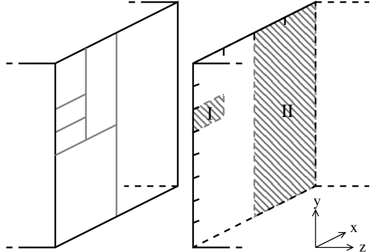
In order to further enhance computational performance, all combinations of and the integrals arising form the stiffness terms of (18) are evaluated and tabulated as well. Precomputing the interface integrals maintains the high computational efficiency of the DG methods also for non-regular grids. Using matrix notation, the semi-discrete DG Maxwell equations (18) read
| (24) |
where S and Z denotes the stiffness and impedance matrix. The matrix operator on the right hand side of (24) represents a weak DG curl operator. Choosing as either zero or one yields centered or upwind fluxes, respectively. By applying centered fluxes the Hamiltonian structure of Maxwell’s equations in continuum is preserved, whereas upwind fluxes lead to a mixed form. Symplectic explicit time integration can be applied in the former case but not in the latter one [18]. For examples of symplectic time integration for Maxwell’s equations in the DG framework see, e.g., [6, 8, 19]. In [3, 5] upwind fluxes and Runge-Kutta schemes are applied for the time integration, where the latter one is concerned with Maxwell’s equations.
3 Local refinement techniques
The adaptation techniques presented in the following are based on projections between the finite element spaces introduced in (12). The projection operators have been introduced in [16], however, they are included for completeness. Also, we address the issue of stability in depth and amended this section with examples.
The approximation to a given function in the FES is obtained by performing an orthogonal projection. The projection is carried out in an element-wise manner, by means of the projection operator given by
| (25) |
where denotes the inner product on the element with the associated 2-norm . When applied successively to all elements and all components of given initial conditions of the electric field, , and the magnetic field, , the respective DG approximations and are obtained. These approximations are optimal in the sense that the projection errors are orthogonal to the space of basis functions
| (26) |
3.1 -Refinement
As stated above -refinement is achieved by means of element bisections along the coordinate directions, where we allow for anisotropic refinements. The refined elements are referred to as the left and right hand side element and with basis functions denoted as and spanning the spaces and in a full analogy to defined in (12). The approximation orders and in each child element do not have to be identical, neither are they required to be equal to the respective order of the parent element. The direct sum of the spaces and is denoted by
| (27) |
In the following, the projection (25) can be applied in order to project an approximation given in an element to the FES associated with an -refined or -reduced element. For -refinement this yields
| (28) |
Due to the tensor product character of the basis, this can be expressed as
| (29) |
for the left and right child, respectively. If refinement is carried out along one coordinate only, e.g. , this further simplifies to
| (30) |
where denotes the Kronecker delta. Note that above we loop over , whereas in (29) the loop parameter is . As, moreover, vanishes for any , we can limit the above loop to the range , which reduces the number of addends to the minimum possible.
3.2 -Refinement
For the case of -enrichments, the local FES are amended with the order basis functions
| (32) |
where any (non-zero) number of the local maximum approximation orders may be increased. Also, an enrichment by more than one higher order basis function is possible. Formally, we perform the orthogonal projection (25), however, due to the orthogonality property of the basis functions the coefficients remain unaltered under a projection from to . Practically, we simply extend the local vectors of coefficients with the new coefficients , which are initialized to zero.
Conversely, for the case of a -reduction, the local FES is reduced by discarding the -order basis functions
| (33) |
Again, by virtue of the orthogonality, we find that the coefficients are deleted from the local vectors of coefficients while the coefficients remain unaltered.
We denote by the projection of the global approximation from the current discretization to another one obtained by local - and -adaptations.
3.3 Optimality, Efficiency and Stability
3.3.1 Optimality
An approximation with coefficients according to (25) is optimal in the sense of (26). The approximations within refined and merged elements with coefficients obtained through the orthogonal projections (28) and (31) are, hence, optimal in the same sense.
If and holds true for all , the FES is a subspace of (cf. (27)) and every function of is representable in but not vice versa. In this case, a given approximation is exactly represented within an element under -refinement but not under -reduction. See Fig. 2 for an example.

3.3.2 Efficiency
Since the projections (28) for performing -refinement are independent of the actual approximation, we also tabulated the projection operators and (expressed in master basis functions) yielding the matrix operators and , where the superscript denotes that the refinement level is increased. Accordingly, we make use of the matrix operators and for evaluating the projections of (31) in the case of element merging. The matrix operators are related as
| (34) |
This allows for the computation of the approximations within adapted elements by means of efficient matrix-vector multiplications. As all projection matrices are triangular the evaluation can be carried out as an in-place operation requiring no allocation of temporary memory.
3.3.3 Stability
The global approximation associated with an adapted grid is computed as . It can be considered as initial conditions applied on the new discretization obtained by performing the refinement operations. Assuming stability of the time stepping scheme (cf. [5, 6, 8]), it is sufficient to show that the application of the projection operators at some time does not increase the electromagnetic energy associated with the approximate DG solution, i.e.,
| (35) |
In this case it follows and, thus, stability of the adaptive scheme.
Following (3) the energy associated with element is given as
| (36) |
As a consequence of (29), it is sufficient to show that the energy (36) is non-increasing during any adaptation involving one coordinate only.
-Refinement
For the following discussion of stability it is assumed that refinement is carried out along the -coordinate. Also we assume the maximum approximation orders and to be identical. It is clarified later, that this does not pose a restriction to the general validity of the results.
In the case of -refinement, the operators and project from the space to the larger space . Following the argument of paragraph 3.3.1 on optimality, any function defined in the space is exactly represented in . The conservation of the discrete energy is a direct consequence as the approximation in the parent and child elements are point-wise identical11 1 Identical material properties are assumed for the parent and child elements..
We find the following relation for the 2-norms of the respective local vectors of coefficients
| (37) |
The exemplary parent element approximation plotted in Fig. 2a has a maximum order of with all coefficients equal to one. The coefficients of the child element approximations and the square values of their 2-norms are given in Tab. 1. If the vector is considered to be either the vector of coefficients of the electric field or the magnetic field the result agrees with (37).
| -1.0000 | -1.0000 | -1.0000 | -1.0000 | -1.0000 | -1.0000 | -1.0000 | 7.0000 | |
| -0.2574 | -0.1355 | -0.2606 | -0.1446 | -0.4276 | -0.1563 | -0.0156 | 0.3808 | |
| -1.7426 | -1.5631 | -1.6819 | -2.0399 | -1.0494 | -0.2181 | -0.0156 | 13.6192 |
The -coarsening operators and project a function from the space to the smaller space . Since is a subspace of , it is immediately concluded that, in general, energy is lost during the coarsening process. The discrete energy can only be preserved if the union of the left and right hand functions is an element of the smaller space . Starting with the coefficients of the child elements, given in Tab. 1, the parent element coefficients are exactly recovered and the discrete energy is preserved.
In particular, it can be shown from algebraic properties of the projection matrices, that the discrete energy for arbitrary fine grid coefficients is always non-increasing during -coarsening. First, the projection matrix is defined as
| (38) |
The coefficients of the child elements are gathered in one vector
| (39) |
Then, the coefficients of the parent element are given as
| (40) |
which is equivalent to Eqn. (31). Using (36) and (37), the following must hold true in order to guarantee a non-increasing discrete energy
| (41) |
In order to fulfill this it is sufficient to demand
| (42) |
Since the matrix has the -times degenerated eigenvalues and this is always fulfilled.
The coefficients for the example shown in Fig. 2b are listed in Table 2. The sum of the 2-norms for the left and right hand child vectors of coefficients yields 1.9003 while twice the value obtained for the parent element evaluates to 1.8996. Thus, energy was lost during -coarsening.
| 0.9500 | -0.0433 | -0.2073 | -0.0498 | 0.9498 | |
| 1.0000 | -0.2000 | -0.1000 | -0.0100 | 1.0501 | |
| 0.9000 | -0.2000 | -0.0100 | -0.0100 | 0.8502 |
-Refinement
In order to show stability of the -adaptation we again consider the energy stored in an element given by (36). In the case of -enrichment, the local vectors of DoF are extended by the coefficients corresponding to the -order basis functions. Since these coefficients are initialized to zero, it holds true
| (43) |
The discrete energy is exactly conserved.
In the case of a -reduction, the coefficients assigned to the highest order basis functions are removed from the vectors of DoF. Consequently, it holds true
| (44) |
and the discrete energy is either preserved or otherwise reduced. If the decision for reducing the order is a correct one, the highest order coefficients are small and the induced energy loss is small.
In the discussion of stability for -adaptations it was assumed that the maximum approximation orders and are identical. After showing that -adaptation does not increase the electromagnetic energy either, it can be concluded that this assumption does not restrict the validity of the results obtained as the problem can be reduced to performing - and -adaptations sequentially.
Finally, we will make some remarks on mixed - and -adaptations. If an -coarsening goes along with a -enrichment, the latter should be performed first. It amounts to a projection to the superspace . Projection errors are limited to the projection onto the space . If the projections are carried out in reversed order the final space is as well, however, the second projection from adds zeros to the local vector of DoF only, resulting in an increased overall projection error. On the contrary, if an -refinement goes along with a -reduction, the former should be carried out first for the same reason. However, the two adaptations can be performed simultaneously by employing projection matrices of the size .
4 Automatic -adaptivity: Error and smoothness estimation
In the preceding section we presented efficient techniques for performing local - and -adaptations, which can be considered as the basic toolbox within the larger frame of an -adaptive DG method. In this section we address the critical issues of locally estimating the approximation error and solution smoothness, which is required for driving the adaptation process. Note that as we are interested in estimating the smoothness of the actual solution, the discontinuous nature of the DG approximation is not a concern. In fact, we will show how the discontinuities at element boundaries can be exploited for constructing a smoothness indicator.
In order to perform an adaptation of an -mesh two steps have to be carried out. First, the elements requiring adaptation have to be identified. This is achieved by an element-wise error estimation. If the estimate exceeds some tolerance the element requires refinement, elements having a small error are eligible for coarsening. In a second step, the kind of adaptation ( or ) suitable for the respective element has to be decided upon. Here, we distinguish between the refinement and the coarsening case.
For the coarsening case the best option is obtained by consecutively testing possible de-refinements from a set of candidates [20, 21]. The set contains at least the candidates obtained by -reducing the refinement level to and by reducing the polynomial order to but larger sets of candidates are possible as well. The list of candidates can be extended hierarchically. If, e.g., reducing the polynomial order yields an approximation still fulfilling the accuracy requirements, subsequent candidates can be generated as long as the accuracy demands are met.
An extension to the refinement case is possible as shown in [22, 20, 21], however, at the price of computing a globally - and -refined solution. We pursued a different approach based on a local smoothness indicator (cf. Sec. 4.2).
4.1 Error Estimation
Error estimation is addressed in a large number of publications out of which we refer to the introductions [23, 24] and references therein. In the context of this paper, we focus on [25], where a relation between the size of the jumps of some quantity at element boundaries
| (45) |
and the residual within in the respective element is derived for a model problem. Following this idea, we obtained a similar result for Maxwell’s equations, which we apply as an error estimate. This is a valuable tool for the development of an adaptive DG method because the evaluation of the jumps is a computationally inexpensive operation. Moreover, it can be incorporated with the computation of the fluxes, which renders the extra costs negligible. The derivation is outlined in the following.
The starting point is equation (18a), where we integrate the second term of the volume integral by parts to obtain
| (46) |
where we returned to denoting the test function by (cf. (5)) for emphasizing the freedom of choice. Taking we obtain
| (47) |
with the residual
| (48) |
and the element error estimate
| (49) |
The global error estimate is obtained as . By inserting either of the fluxes (15) or (16), i.e. centered or upwind, in (47) we obtain
| (50a) | ||||
| (50b) | ||||
where numbers all interfaces of element . This establishes the link between the jump sizes and the residual. Note, that there is a consistency with the observation that in homogeneous regions the jumps disappear if the numerical solution is exact.
Figure 3 shows results of tests we conducted for investigating the estimate performance. The tests were carried out in a one-dimensional domain using a Gaussian and a trapezoidal wave form as examples for a smooth solution and non-smooth solution. Bold lines in Fig. 3 correspond to the global approximation error in the -norm, dashed lines represent the global error estimate .
The estimate performs well for the Gaussian wave form. It tends to overestimate the error, however, we consider the discrepancies to be acceptable, especially given that it reproduces the correct trend under grid refinement. The situation is not as good for the trapezoidal wave form, where the overestimation of the error is more significant. Nevertheless, also for this example the trend under grid refinement is correct.

4.2 Smoothness Estimation
Once an element is marked for refinement, it has to be decided upon the kind of adaptation to perform. This -decision is based on the solution smoothness. If the approximation within the element under consideration is sufficiently smooth we perform -refinement in order to obtain spectral convergence [26, 27]. Otherwise, we choose -refinement. Hence, the discretization error and the achievable order of convergence critically depend on correct -decisions. This in turn makes reliable smoothness estimators a necessity for adaptive codes.
The subject of smoothness estimation has a good coverage in the literature as well. In one of the first publications on adaptive DG methods [28] the authors propose to estimate the local solution regularity based on the decay rate of the local error. As the local error is unknown and subject to estimation itself the adaptation procedure critically hinges on the error estimate. More recent works such as [29, 30, 31, 32, 33, 34] attempt to estimate the solution smoothness based on a variety of properties of the local solution, but they do not include the error estimate. See [29] also for a more complete overview of different smoothness estimation concepts.
A first family of popular methods estimates the local analyticity by projecting the solution to a set of orthogonal functions (e.g. Legendre polynomials) and investigates the decay of the coefficients in on way or another. This approach is being followed by [29, 31, 32, 33], where the latter one builds on top of [31] and obtains improved results especially when the sequence of coefficients exhibits a pronounced odd-even behavior. As we express the approximation as a Legendre series within each element the projection step would not be required. In [29, 34] the authors attempt to estimate the local Sobolev regularity index directly, where the former one requires the representation of the solution as a Legendre series as well whereas the latter one is a novel idea based on continuous Sobolev embeddings and does not require a series expansion. Finally, smoothness indicators can also be built from superconvergence properties of the DG method [35, 30], which will be described in more details below.
The first family of smoothness estimates are mainly applied in the context of shock capturing, specifically for controlling artificial viscosity within high order DG simulations. In this context they proved to reliably achieve a good performance. In our experience, however, they are rather not suited for controlling an -decision as they require a minimum number of coefficients for estimating the decay rate, which might not be available for low order elements.
We adapted the smoothness indicator for hyperbolic conservation laws [30], which exploits the difference in the convergence rate of interface jumps for smooth and non-smooth solutions. From our experience this indicator works very robust and, most importantly, this remains valid down to very low polynomial orders of one and even zero. This coincides with the experiences reported in [36, 37]. It should be noted, however, that no estimated value for the local analyticity or regularity is obtained. We plan to test the estimate [34] since it appears to be working down to low orders while obtaining an estimated regularity index at the same time. For the time being, however, we consider an adapted version of the smoothness indicator [30].
For a scalar quantity that can be a solution component or a derived quantity as well, it holds true [35]
| (51) |
where denotes an outflow boundary regarding the quantity . Following [30] the superconvergence property (51) can be exploited for constructing a smoothness indicator. To this end we consider
| (52) |
As a result of (51) the last integral converges as and the left hand side expression is in regions of smooth solution. If, however, is non-smooth in the vicinity of then both right hand side integrals are only . Normalizing (52) by an average convergence rate and the -norm of the considered quantity on yields a smoothness indicator
| (53) |
where is a characteristic measure of the size of element . We use the length of the edge normal to the interface , which for the one-dimensional case is simply the element length. For the solution on is considered to be non-smooth and smooth otherwise with -refinement being performed in the former case and -refinement in the latter one. As the indicator is applied at element faces, it allows for indicating the solution smoothness along each coordinate separately which can be expoited for driving anisotropic -refinement.
We use components of the Poynting vector as the considered quantity . Then, inflow boundaries are recognized by . The Poynting vector represents the energy flux density. As a consequence of this particular choice, the nominator of (53) is large for big jumps of the energy flux density across the element boundary. This is likely to indicate a low regularity of the local field solution and allows for interpreting the smoothness indicator based on the underlying physics. As this interpretation does not depend on the element order, we assume that this explains our observation of a good performance also for low orders (see Example 5.1).
5 Application examples
In this section we will present two examples of the fully automatic -adaptive solution of wave propagation problems in one-dimensional space and one example which proves the capability of our implementation to handle large problems in three-dimensional space including thousands of mesh adaptations. However, in the latter example we drive the adaptation using a simple energy density criterion for the practical reason that the implementation of the estimates for the three-dimensional case is not yet completed.
5.1 Automatic adaptation in one-dimensional space
The adaptation strategy described above is being tested with a Gaussian and a trapezoidal wave packet in a one-dimensional setting as shown in Fig. 4. The error tolerances are for the former and for the latter case. The gray dashed lines depict the position of the grid points and the red circles indicate the approximation order employed for the respective element divided by ten. For the Gaussian packet the adaptation algorithm chooses medium sized to big elements and the preset maximum approximation order of five in the vicinity of the packet. For the non-smooth trapezoidal packet, the maximum approximation order chosen by the algorithm throughout the simulation is two. In the vicinity of the pulse edges a high degree of -refinement is applied, thus showing the desired behavior for the second packet as well.
Figure 5 shows a comparision of the -error achieved for varying numbers of DoF using -adaptivity (corresponding to different error tolerances) and fixed meshes of uniform polynomial order. Using -meshes the number of DoF required for obtaining a certain accuracy is clearly reduced. The achievable gain by using -adaptivity, however, strongly depends on the problem under consideration. For the examples considered here, e.g., enlarging the domain while preserving the size of the wave packet will increase the separation between the curves corresponding to the adaptive and non-adaptive solutions in favor of the -solution and vice versa. In other words, the more pronounced the multiscale character of the problem is the higher is the gain by applying -adaptivity.


5.2 Proof of feasibility example in three-dimensional space
In this section we consider the backscattering of a wide-band electromagnetic pulse from a passive radar reflector. As stated above, the implementation of the error and smoothness estimates for applications in three-dimensional space is underway, and we resorted to applying a physics based criterion for driving the mesh adaptation process. The purpose of this example is to demonstrate the ability of our implementation [38] to handle large scale problems using -meshes. This involves the handling of meshes with hanging nodes and thousands of adaptations on the element level, which are carried out by means of the efficient techniques presented above.
In this example a radar reflector is illuminated off-center by a horn antenna, which emits a Gaussian-modulated sinusoidal pulse covering the frequency range from 20 to 30 GHz. The initial waveform is a TE10 (transverse electric) wave. The setup is depicted in Fig. 6, where the antenna is shown in a cut view along with contour plots of the pulse at two instances in time ( ns and ns). Table 3 lists the parameters and dimensions. We simulated the full scattering process starting from the excitation inside the waveguide to the recording of the reflected fields at the same position. The total propagation distance is about sixty wavelengths.

| Parameter | Value |
|---|---|
| Waveform mode | TE10 |
| Waveform frequency range | 20 – 30 GHz |
| Waveguide type | WR-62 |
| Waveguide width | 15.8 mm |
| Waveguide height | 7.9 mm |
| Horn width | 39.7 mm |
| Horn height | 29.0 mm |
| Horn depth | 67.5 mm |
We chose a maximum -refinement level of two and the local element order to vary in between zero and four. The local energy density, introduced in (3), serves as the criterion for controlling the adaptation procedure. Denoting by the average energy density of element and by the normalized energy density with , we assigned the local refinement levels according to and polynomial orders as with .
The initial discretization consisted of elements. During the simulation the number of elements varies and grew strongly after scattering from the reflector took place, when it reached close to 800,000 elements corresponding to slightly more than 55 million DoF. For comparison, we note that employing the finest mesh resolution globally as well as fourth order approximations uniformly would lead to approximately 7.5 billion () DoF. This corresponds to a factor of approximately 130 in terms of memory savings. We emphasize that the simulations were carried out on a single machine. The implementation takes full advantage of multi-core capabilities through OpenMP parallelization. The numerous run-time memory allocations and deallocations are handled through a specialized memory management library based on memory blocking, which we implemented for supporting the main code [39].
Figure 7 depicts cut-views of the -component of the electric field and the respective -mesh at three instances in time. Note that the scaling of the electric field differs for every time instance, which is necessary to allow for a visual inspection. The enlargement shows details of the computational grid. All elements are of hexahedral kind, however, we make use of the common tensor product visualization technique (cf. [40, 41]) using embedded tetrahedra for displaying the three tensor product orders (out of which only and are visible in the depicted -plane). As we employed isotropic - as well as -refinement all tetrahedra associated with one element share the same color. Figure 8 shows plots of the outgoing and reflected waveform recorded along the waveguide center. The blue dashed line was obtained with the commercial CST Microwave Studio software [42] on a very fine mesh and serves as a cross comparison result.


6 Conclusions
We presented a discontinuous Galerkin formulation for non-regular hexahedral meshes and showed that hanging nodes of high level can easily be included into the framework. In fact, any non-regularity of the grid can be included in a single term reflecting the contribution of neighboring elements to the local interface flux. We demonstrated that the method can be implemented such that it maintains its computational efficiency also on non-regular and locally refined meshes as long as the mesh is derived from a regular root tesselation by means of element bisections. This is achieved by extensive tabulations of flux and projection matrices, which are obtained through (analytical) precomputations of integral terms.
We also presented local refinement techniques for - and -refinements, which are based on projections between finite element spaces. These projections were shown to guarantee minimal projection errors in the -sense and to lead to an overall stable time-domain scheme.
Local error and smoothness estimates have been addressed, both of them relate to the size of the interface jumps of the DG solution. We considered the simulation of a smooth and a non-smooth waveform in a one-dimensional domain for validating the error and smoothness estimates.
As an application example in three-dimensional space the backscattering of a broadband waveform from a radar reflector was considered. In this example the total wave propagation distance corresponds to approximately sixty wavelengths involving thousand of local mesh adaptations. As the implementation of the derived error and smoothness estimates for three-dimensional problems is subject of ongoing work, we chose to drive the grid adaptation using the energy density as refinement indicator. Crosschecking with a result obtained using a commercial software package showed good agreement.
References
- [1] W. Reed, T. Hill, Triangular mesh methods for the neutron transport equation, Tech. rep., Los Alamos Scientific Laboratory Report (1973).
- [2] P. LeSaint, P.-A. Raviart, On a finite element method for solving the neutron transport equation, Academic Press, 1974, pp. 89–123.
- [3] B. Cockburn, C. Shu, Runge–kutta discontinuous galerkin methods for convection-dominated problems, J Sci Comput 16 (3) (2001) 173–261.
- [4] J. S. Hesthaven, T. Warburton, Nodal Discontinuous Galerkin Methods, Springer, 2008.
- [5] J. S. Hesthaven, T. Warburton, Nodal high-order methods on unstructured grids i. time-domain solution of maxwell’s equations, J Comput Phys 181 (1) (2002) 186–221.
- [6] L. Fezoui, S. Lanteri, S. Lohrengel, S. Piperno, Convergence and stability of a discontinuous galerkin time-domain method for the 3d heterogeneous maxwell equations on unstructured meshes, ESAIM-Math Model Num 39 (6) (2005) 1149–1176.
- [7] G. Cohen, X. Ferrieres, S. Pernet, A spatial high-order hexahedral discontinuous Galerkin method to solve Maxwell’s equations in time domain, J Comput Phys 217 (2) (2006) 340–363.
- [8] E. Gjonaj, T. Lau, S. Schnepp, F. Wolfheimer, T. Weiland, Accurate modelling of charged particle beams in linear accelerators, New J Phys 8 (2006) 1–21.
- [9] D. Wirasaet, S. Tanaka, E. J. Kubatko, J. J. Westerink, C. Dawson, A performance comparison of nodal discontinuous galerkin methods on triangles and quadrilaterals, Int J Numer Meth Fluids 64 (10-12) (2010) 1336–1362.
- [10] K. Bey, J. Oden, hp-version discontinuous galerkin methods for hyperbolic conservation laws, Comput Method Appl M 133 (1996) 259–286.
- [11] C. Baumann, J. Oden, A discontinuous hp finite element method for convection–diffusion problems, Comput Method Appl M 175 (3-4) (1999) 311–341.
- [12] P. Houston, E. Süli, hp-adaptive discontinuous galerkin finite element methods for first-order hyperbolic problems, SIAM J Sci Comput 23 (2001) 1226–1252.
- [13] I. Perugia, D. Schötzau, P. Monk, Stabilized interior penalty methods for the time-harmonic maxwell equations, Comput Method Appl M 191 (41) (2002) 4675–4698.
- [14] I. Perugia, D. Schotzau, The hp-local discontinuous galerkin method for low-frequency time-harmonic maxwell equations, Math Comput 72 (243) (2003) 1179–1214.
- [15] P. Houston, I. Perugia, D. Schotzau, Energy norm a posteriori error estimation for mixed discontinuous galerkin approximations of the maxwell operator, Comput Method Appl M 194 (2-5) (2005) 499–510.
- [16] S.M. Schnepp, T. Weiland, Discontinuous galerkin methods with transient hp-adaptation, Radio Sci 46 (2011) RS0E03.
- [17] R. J. LeVeque, Numerical Methods for Conservation Laws, Birkhäuser, 1990.
- [18] S. Schnepp, E. Gjonaj, T. Weiland, A hybrid finite integration–finite volume scheme, J Comput Phys 229 (11) (2010) 4075–4096.
- [19] N. Canouet, L. Fezoui, S. Piperno, Discontinuous galerkin time-domain solution of maxwell’s equations on locally-refined nonconforming cartesian grids, COMPEL 24 (4) (2005) 1381–1401.
- [20] L. Demkowicz, J. Oden, W. Rachowicz, Toward a universal hp adaptive finite element strategy, part 1. constrained approximation and data structure, Comput Method Appl M 77 (1-2) (1989) 181–212.
- [21] P. Solin, L. Dubcova, J. Cerveny, I. Dolezel, Adaptive hp-fem with arbitrary-level hanging nodes for maxwell’s equations, Advances in Applied Mathematics and Mechanics 2 (4) (2010) 518–532.
- [22] W. Rachowicz, J. T. Oden, L. Demkowicz, Toward a universal h-p adaptive finite element strategy part 3. design of h-p meshes, Comput Method Appl M 77 (1-2) (1989) 181–212.
- [23] M. Ainsworth, J. T. Oden, A posteriori error estimation in finite element analysis, Wiley-Interscience, 2000.
- [24] B. Cockburn, A simple introduction to error estimation for nonlinear hyperbolic conservation laws, School of Mathematics, University of Minnesota.
- [25] B. Cockburn, Discontinuous galerkin methods, ZAMM-Z Angew Math Me 83 (11) (2003) 731–754.
- [26] I. Babuska, The p and hp versions of the finite element method, basic principles and properties, SIAM review.
- [27] C. Schwab, p- and hp- Finite Element Methods: Theory and Applications to Solid and Fluid Mechanics, Oxford University Press, USA, 1999.
- [28] K. Bey, J. Tinsley Oden, A. Patra, A parallel hp-adaptive discontinuous Galerkin method for hyperbolic conservation laws, Appl Numer Math 20 (4) (1996) 321–336.
- [29] P. Houston, E. Suli, A note on the design of hp-adaptive finite element methods for elliptic partial differential equations, Comput Method Appl M 194 (2-5) (2005) 229–243.
- [30] L. Krivodonova, J. Xin, J. Remacle, N. Chevaugeon, J. Flaherty, Shock detection and limiting with discontinuous Galerkin methods for hyperbolic conservation laws, Appl Numer Math 48 (3-4) (2004) 323–338.
- [31] P.-O. Persson, J. Peraire, Sub-cell shock capturing for discontinuous galerkin methods, Proc. of the 44th AIAA Aerospace Sciences Meeting and Exhibit 112 (2006).
- [32] E. Casoni, J. Peraire, A. Huerta, One-dimensional shock-capturing for high-order discontinuous galerkin methods, ECCOMAS Multidisciplinary Jubilee Symposium (2009) 307–325.
- [33] A. Klöckner, T. Warburton, J. S. Hesthaven, Viscous shock capturing in a time-explicit discontinuous Galerkin method, Mathematical Modelling of Natural Phenomena 6 (3) (2011) 57–83.
- [34] T. P. Wihler, An hp-adaptive strategy based on continuous Sobolev embeddings, J Comput Appl Math 235 (8) (2011) 2731–2739.
- [35] S. Adjerid, K. Devine, J. Flaherty, L. Krivodonova, A posteriori error estimation for discontinuous Galerkin solutions of hyperbolic problems, Comput Method Appl M 191 (11-12) (2002) 1097–1112.
- [36] H. Luo, J. Baum, R. Löhner, On the computation of steady-state compressible flows using a dg method, Computational Fluid Dynamics 2006 (2009) 47–52.
- [37] A. Richter, J. Stiller, R. Grundmann, Stabilized high-order discontinuous galerkin methods for aeroacoustic investigations, Computational Fluid Dynamics 2008 (2009) 77–82.
- [38] SMOVE, A program for the adaptive simulation of electromagnetic fields and arbitrarily shaped charged particle bunches using moving meshes, technical documentation: http://www.graduate-school-ce.de/files2/schnepp/SMOVE/.
- [39] DynaMO, A dynamic memory organization library, technical documentation: http://www.graduate-school-ce.de/files2/schnepp/DynaMO/.
- [40] P. Solin, J. Cerveny, I. Dolezel, Arbitrary-level hanging nodes and automatic adaptivity in the hp-fem, Math Comput Simulat 77 (1) (2008) 117 – 132.
- [41] L. Demkowicz, Computing with HP-Adaptive Finite Elements: Volume 1: One and Two Dimensional Elliptic and Maxwell Problems, Chapman & Hall/CRC, 2007.
- [42] CST AG, Bad Nauheimer Str. 19, 64289 Darmstadt, Germany.