跳到论文正文
W Papers独立论文阅读器 arXiv:1109.0827 论文正文 计算阅读时间 · 0%
引用这篇论文根据当前论文元数据生成,正式投稿前建议核对。


License: arXiv.org perpetual non-exclusive license
arXiv:1109.0827v1 [cs.IT] 05 Sep 2011

A Trellis Coded Modulation Scheme for the Fading Relay Channel

Vijayvaradharaj T Muralidharan Affiliation: Dept. of ECE, Indian Institute of Science
Bangalore 560012, India
Email: tmvijay@ece.iisc.ernet.in
   B. Sundar Rajan Affiliation: Dept. of ECE, Indian Institute of Science,
Bangalore 560012, India
Email: bsrajan@ece.iisc.ernet.in
Abstract

A decode and forward protocol based Trellis Coded Modulation (TCM) scheme for the half-duplex relay channel, in a Rayleigh fading environment, is presented. The proposed scheme can achieve any spectral efficiency greater than or equal to one bit per channel use (bpcu). A near-ML decoder for the suggested TCM scheme is proposed. It is shown that the high SNR performance of this near-ML decoder approaches the performance of the optimal ML decoder. The high SNR performance of this near-ML decoder is independent of the strength of the Source-Relay link and approaches the performance of the optimal ML decoder with an ideal Source-Relay link. Based on the derived Pair-wise Error Probability (PEP) bounds, design criteria to maximize the diversity and coding gains are obtained. Simulation results show a large gain in SNR for the proposed TCM scheme over uncoded communication as well as the direct transmission without the relay. Also, it is shown that even for the uncoded transmission scheme, the choice of the labelling scheme (mapping from bits to complex symbols) used at the source and the relay significantly impacts the BER vs SNR performance. We provide a good labelling scheme for 2l2^{l}-PSK signal set, where l≥2l\geq 2 is an integer.

I PRELIMINARIES AND BACKGROUND

Refer to caption
Fig. 1: The Relay Channel

We consider the Rayleigh fading relay channel shown in Fig. 1, consisting of the source node SS, the relay node RR and the destination node DD. It is assumed that R can operate only in the half-duplex mode, i.e., it cannot receive and transmit simultaneously in the same frequency band. It is assumed that R has perfect knowledge about the instantaneous value of the fade coefficient associated with the S-R link and D has perfect knowledge about the instantaneous values of the fade coefficients associated with the S-R, R-D and S-D links. Throughout, the phase during which the relay is in reception mode is referred to as Phase 1 and the phase during which the relay is in transmission mode is referred to as Phase 2.

In all practical scenarios the S-R and R-D links are stronger than the S-D link. As a result, the use of coding schemes which involve both S and R, can potentially outperform the coding schemes involving S alone. The problem addressed in this paper is the design of a Trellis Coded Modulation (TCM) scheme for the relay channel, which achieves a spectral efficiency greater than or equal to one bit per channel use (bpcu) and provides a large gain compared to the TCM scheme for the direct transmission without the relay.

A comparison of the proposed TCM scheme is made with the uncoded transmission scheme for the relay channel operating in the Decode and Forward (DF) mode, in which no coding is done at S and R, which is described as follows: At S, uncoded bits are directly mapped onto complex symbols from a signal set during Phase 1 and transmitted. During Phase 2, S and R map the uncoded bits (S uses the same bits as in Phase 1 and R uses the bits it decoded during Phase 1) onto complex symbols from a signal set for transmission. The signal sets used at S during Phase 1, S during Phase 2 and R during Phase 2 are assumed to be the same, but the mapping from bits to complex symbols can be different.

I-A The Proposed Scheme

Refer to caption
(a) Phase 1
Refer to caption
(b) Phase 2
Fig. 2: The TCM Scheme

The proposed TCM scheme for the fading relay channel is shown in Fig. 2(a) and Fig. 2(b) (shown at the top of the next page). It is assumed that TCM encoding at S during Phase 1 and Phase 2 and at R during Phase 2 take place using the same encoder, but the labelling schemes used for mapping coded bits onto signal points can be different. By a trellis, we refer to the states of the TCM encoder, the edges connecting these states in two successive stages and the complex numbers which are labelled on these edges. By a path in the trellis, we refer to the sequence of connected edges (the complex numbers labelled on the edges are not included). Let 𝒯S1\mathcal{T}_{S_{1}}, 𝒯S2\mathcal{T}_{S_{2}} and 𝒯R\mathcal{T}_{R} represent the trellises used for encoding by S during Phase 1, by S during Phase 2 and by R during Phase 2 respectively. Since the encoder corresponding to the trellises 𝒯S1\mathcal{T}_{S_{1}}, 𝒯S2\mathcal{T}_{S_{2}} and 𝒯R\mathcal{T}_{R} are the same, they differ only in the complex numbers labelled on the edges. Let ζ{\zeta} denote the set of edges connecting the states in two successive stages of the trellis. The labelling of the edges in the trellis 𝒯S1\mathcal{T}_{S_{1}} is given by the map 𝒳s1:ζ⟶𝒮\mathcal{X}_{s_{1}}:\zeta\longrightarrow\mathcal{S}, where 𝒮\mathcal{S} is the signal set used at S and R. Similarly, the maps 𝒳s2\mathcal{X}_{s_{2}} and 𝒳r\mathcal{X}_{r} are defined for the the trellises 𝒯S2\mathcal{T}_{S_{2}} and 𝒯R\mathcal{T}_{R} respectively.

During Phase 1, input bits at SS are encoded by the TCM encoder, mapped onto complex symbols from the signal set 𝒮\mathcal{S} and interleaved by the block interleaver as shown in Fig. 2(a). Each transmission made is assumed to be a block of LL complex symbols. After each transmission, the encoder state is brought back to the all zeros state by appending zero input bits at the end. Let 𝒫S\mathcal{P}_{S} denote the path in the trellis corresponding to the output of the TCM encoder at S. Let xs1i​(𝒫S)x_{s_{1}}^{i}(\mathcal{P}_{S}) denote the symbol to be transmitted corresponding to the it​hi^{th} branch of the path 𝒫S\mathcal{P}_{S}, where 1≤i≤L1\leq i\leq L.

The received complex signal sequence at R and D during Phase 1 are given by,

Yri=hs​ri​xs1i​(𝒫S)+zr;Yd1i=hs​d1i​xs1i​(𝒫S)+zd1;}​1≤i≤L\displaystyle\left.\begin{array}[]{ll}Y_{r}^{i}&=h_{sr}^{i}x_{s_{1}}^{i}(\mathcal{P}_{S})+z_{r};\\ Y_{d_{1}}^{i}&=h_{sd_{1}}^{i}x_{s_{1}}^{i}(\mathcal{P}_{S})+z_{d_{1}};\end{array}\right\}1\leq i\leq L

where hs​rih_{sr}^{i} and hs​d1ih_{{sd}_{1}}^{i} are the independent zero mean circularly symmetric complex Gaussian fading coefficients associated with the S-R and S-D links respectively with the corresponding variances given by σs​r2\sigma^{2}_{sr} and σs​d2\sigma^{2}_{sd}. The additive noises zrz_{r} and zd1z_{d_{1}} are assumed to be C​N​(0,1)CN(0,1), where C​N​(0,1)CN(0,1) denotes the standard circularly symmetric complex Gaussian random variable. An interleaver with sufficiently large block length is assumed to make the block fading channel appear as a fading channel with independent fade coefficients for successive channel uses. At R, after deinterleaving, an ML decoder using the Viterbi algorithm is used to decode the bits (Fig. 2(a)). Let 𝒫R\mathcal{P}_{R} denote the path in the trellis to which R decodes. At D, the received complex numbers are deinterleaved and stored (Fig. 2(a)).

During Phase 2, S encodes the same bits used during Phase 1 and R encodes the bits it decoded during Phase 1, using the TCM encoder. The encoded bits at S and R are mapped onto complex symbols from the signal set 𝒮\mathcal{S} (possibly with different mappings and also possibly different from the mapping used at S during Phase 1) and interleaved using the block interleavers (same as the interleaver used at S during Phase 1) as shown in Fig. 2(b). Let xs2i​(𝒫S)x_{s_{2}}^{i}(\mathcal{P}_{S}) and xri​(𝒫R)x_{r}^{i}(\mathcal{P}_{R}) denote the symbols transmitted by S and R respectively during Phase 2, corresponding to the it​hi^{th} branch of the paths 𝒫S\mathcal{P}_{S} and 𝒫R\mathcal{P}_{R}, where 1≤i≤L1\leq i\leq L.

The received complex signal sequence at D during Phase 2 is given by,

Yd2i\displaystyle Y_{d_{2}}^{i} =hs​d2i​xs2i​(𝒫S)+hr​di​xri​(𝒫R)+zd2,\displaystyle=h_{sd_{2}}^{i}x_{s_{2}}^{i}(\mathcal{P}_{S})+h_{rd}^{i}x_{r}^{i}(\mathcal{P}_{R})+z_{d_{2}},

where 1≤i≤L1\leq i\leq L. The random variables hs​d2ih_{sd_{2}}^{i} and hr​dih_{rd}^{i} are the independent zero mean circularly symmetric complex Gaussian fading coefficients associated with the S-D and R-D links respectively with the corresponding variances given by σs​d2\sigma^{2}_{sd} and σr​d2\sigma^{2}_{rd}. The additive noise zd2z_{d_{2}} is C​N​(0,1)CN(0,1). Throughout, it is assumed that σs​d2≪σr​d2\sigma^{2}_{sd}\ll\sigma^{2}_{rd}, due to the proximity of the relay to the destination than the source to the destination.

During Phase 2, at D the received complex numbers are deinterleaved and along with the complex numbers stored during Phase 1 are fed to the proposed near-ML TCM decoder described in Section III.

I-B Background and Related Work

Achievable rates and upper bounds on the capacity for the discrete memoryless relay channel for the full-duplex and the more practical half-duplex relay channel were obtained in [1],[2]. These results were extended for the half duplex Gaussian relay channel in [3]. Optimal power allocation strategies to maximize the achievable rate for the Rayleigh fading relay channel were investigated in [4]. Several protocols like Amplify and Forward (AF), Decode and Forward (DF), Compress and Forward (CF) were proposed [5]. Power allocation strategies for the Non Orthogonal DF (NODF) protocol were discussed in [6]. Non-orthogonal relay protocols offer higher spectral efficiency when compared with orthogonal relay protocols [7], [8], [9]. Hence, the proposed TCM scheme in this paper is based on the NODF protocol.

A turbo-coding scheme for the full duplex and more practical half-duplex relay channels were proposed in [10],[11]. These coding schemes achieve a spectral efficiency strictly less than one bpcu, i.e., they pay in bandwidth. Coding schemes for the relay channel with bandwidth constraints, which achieve a spectral efficiency greater than or equal to one bpcu are not reported in the literature, to the best of our knowledge. In this paper, we propose a Trellis Coded Modulation (TCM) scheme for the half-duplex relay channel for any spectral efficiency greater than or equal to one bpcu.

Implementation as well as the performance analysis of the optimal ML decoder for the relay channel operating in the DF mode is complicated [12],[13]. To solve these problems, several sub-optimal decoders for uncoded DF scheme were proposed in [12], [13], [14] and [15]. These problems carry over to coded communication using DF protocol as well. If the decoder at D is designed assuming that R always decodes the bits correctly, the diversity order obtained is dependent on whether the relay decoded correctly or not. To circumvent this problem, relay selection strategies [16], fountain codes [17], Cyclic Redundancy Check (CRC) codes [18] etc. are used. To solve these problems of finding a decoder with implementable complexity and tractable performance analysis, we propose a near-ML decoder, whose performance at high SNR approaches the performance of the optimal ML decoder. The form of this decoder allows a DF scheme in which the relay need not check whether it has decoded correctly before forwarding the message. This eliminates the need for embedding CRC bits as well as the need for feedback from the relay to the source. Furthermore, the diversity order of the proposed scheme does not depend on whether the relay decoded correctly or not.

The proposed TCM scheme is different from the Co-operative Multiple Trellis Coded Modulation (CMTCM) scheme proposed in [18] in the following aspects:

  • •

    The presence of embedded CRC bits and feedback from R to S is assumed in [18], whereas we make no such assumptions.

  • •

    Interleaving/Deinterleaving is not assumed in [18] whereas we assume interleaving/deinterleaving which makes the quasi-static fading scenario appear as a fast fading scenario.

I-C Contributions and Organization

The main contributions of this paper are as follows:

  • •

    A TCM scheme for the fading relay channel is proposed which achieves any spectral efficiency greater than or equal to one bpcu.

  • •

    A near-ML decoder is obtained for the proposed TCM scheme. The relay need not check whether it has decoded correctly before forwarding the message which eliminates the need for embedded CRC bits as well as the feedback from the relay to the source.

  • •

    The proposed near-ML decoder enables the formulation of design criteria to maximize the diversity order and the coding gain.

  • •

    Bounds on the PEP are derived for the near-ML decoder based on which the criteria to maximize the diversity order and coding gain are obtained.

  • •

    The BER vs SNR performance of the near-ML decoder proposed with a non-ideal S-R link, at high SNR, approaches the performance of the optimal ML decoder with an ideal S-R link. This implies that the high SNR performance of the near-ML decoder for the relay channel with a non-ideal S-R link approaches the performance of the optimal ML decoder.

  • •

    It is shown that even for the uncoded transmission scheme, a proper choice of the labelling at S and R provides a significant performance improvement. We give a good labelling scheme for 2l2^{l}-PSK signal set, where l≥2l\geq 2 is an integer.

  • •

    Simulation results show a large gain in the BER vs SNR performance for the proposed TCM scheme over the uncoded transmission scheme as well as the TCM scheme for the direct transmission without the relay.

The organization of the rest of the paper is as follows: In Section II, the bounds on the ergodic capacity of the fading relay channel with Gaussian input alphabet are compared with the capacity bounds when the input is constrained to take values from a finite signal set. The description of the near-ML decoder for the TCM scheme constitutes Section III. In Section IV, the PEP expressions are derived, based on which the code design criteria to maximize the diversity order and coding gain are obtained. In Section V, effect of the choice of the labelling scheme for the uncoded transmission scheme is discussed and a good labelling scheme for 2l2^{l}-PSK constellation is presented. In Section VI, TCM code design examples are presented. Simulation results are presented in Section VII.

Notations: For a random variable XsX_{s} which takes value from the set 𝒮\cal S, we use xs,ix_{s,i} to represent the ii-th element of 𝒮\cal S. Ez​[Y]\textbf{E}_{z}[Y] denotes the expectation of YY with respect to the random variable z. Throughout, l​o​glog refers to l​o​g2log_{2} and C⁡(a)C(a) denotes l​o​g​(1+a)log(1+a). Let C​N​(0,In)CN(0,I_{n}) denote the standard circularly symmetric complex Gaussian random vector of length nn. Also let N⁡(0,c)N(0,c) denote the scalar real valued Gaussian random variable with mean zero and variance cc. For simplicity, distinction is not made between the random variable and a particular realization of the random variable, in expressions involving probabilities of random variables. In some probability expressions involving conditioning of the fading coefficients, the fact that the probability is conditioned on the values taken by the fading coefficients is not explicitly written, as it can be understood from the context. For a set 𝒜\mathcal{A}, |𝒜||\mathcal{A}| denotes the cardinality of 𝒜\mathcal{A}. For two sets 𝒜\mathcal{A} and ℬ\mathcal{B}, 𝒜∪ℬ\mathcal{A}\cup\mathcal{B} denotes the union of the sets 𝒜\mathcal{A} and ℬ\mathcal{B}. The superscript (.)T(.)^{T} denotes the transpose operation. The set {x∣c⁡(x)}\{x\mid c(x)\} denotes the set of all values of xx for which the condition c⁡(x)c(x) is satisfied. ℜ⁡(x)\Re(x) denotes the real part of the complex number xx. Throughout, E𝒮E_{\mathcal{S}} denotes the average energy in dB of the signal set 𝒮\mathcal{S} used at the source and the relay. Let Q[.] denote the complementary CDF of the standard Gaussian random variable.

R1≜I(Xs1;Yr)]=log(Ms1)−1Ms1∑i1=0Ms1−1Ezr[log(∑i=0Ms1−1e​x​p​(−|zr−hs​r​xs1,i+hs​r​xs1,i1|2)e​x​p​(−|zr|2))]\displaystyle R_{1}~\triangleq~I(X_{s_{1}};Y_{r})]=log(M_{s_{1}})-\frac{1}{M_{s_{1}}}\sum_{i_{1}=0}^{M_{s_{1}}-1}\textbf{E}_{z_{r}}\left[log\left(\dfrac{\sum_{i=0}^{M_{s_{1}}-1}exp\left(-|z_{r}-h_{sr}x_{s_{1},i}+h_{sr}x_{s_{1},i_{1}}|^{2}\right)}{exp(-|z_{r}|^{2})}\right)\right] (1)
R2≜I(Xs2;Yd2|Xr)]=log(Ms2)−1Ms2∑i1=0Ms2−1Ezd2[log(∑i=0Ms2−1e​x​p​(−|zd2−hs​d​xs2,i+hs​d​xs2,i1|2)e​x​p​(−|zd2|2))]\displaystyle R_{2}~\triangleq~I(X_{s_{2}};Y_{d_{2}}|X_{r})]=log(M_{s_{2}})-\frac{1}{M_{s_{2}}}\sum_{i_{1}=0}^{M_{s_{2}}-1}\textbf{E}_{z_{d_{2}}}\left[log\left(\dfrac{\sum_{i=0}^{M_{s_{2}}-1}exp\left(-|z_{d_{2}}-h_{sd}x_{s_{2},i}+h_{sd}x_{s_{2},i_{1}}|^{2}\right)}{exp(-|z_{d_{2}}|^{2})}\right)\right] (2)
R3≜I(Xs1;Yd1)]=log(Ms1)−1Ms1∑i1=0Ms1−1Ezd1[log(∑i=0Ms1−1e​x​p​(−|zd1−hs​d​xs1,i+hs​d​xs1,i1|2)e​x​p​(−|zd1|2))]\displaystyle R_{3}~\triangleq~I(X_{s_{1}};Y_{d_{1}})]=log(M_{s_{1}})-\frac{1}{M_{s_{1}}}\sum_{i_{1}=0}^{M_{s_{1}}-1}\textbf{E}_{z_{d_{1}}}\left[log\left(\dfrac{\sum_{i=0}^{M_{s_{1}}-1}exp\left(-|z_{d_{1}}-h_{sd}x_{s_{1},i}+h_{sd}x_{s_{1},i_{1}}|^{2}\right)}{exp(-|z_{d_{1}}|^{2})}\right)\right] (3)
R4≜I⁡(Xs2,Xr,Yd2)=l​o​g​(Ms2​Mr)\displaystyle R_{4}~\triangleq~I(X_{s_{2}},X_{r};Y_{d_{2}})=log(M_{s_{2}}M_{r})
−1Ms2​Mr∑i1=0Ms2−1∑j1=0Mr−1Ezd2[log(∑i=0Ms2−1∑j=0Mr−1e​x​p​(−|zd2−hs​d​xs2,i−hr​d​xr,j+hs​d​xs2,i1+hr​d​xr,j1|2)e​x​p​(−|zd2|2))]\displaystyle\hskip 85.35826pt-\dfrac{1}{M_{s_{2}}M_{r}}\sum_{i_{1}=0}^{M_{s_{2}}-1}\sum_{j_{1}=0}^{M_{r}-1}\textbf{E}_{z_{d_{2}}}\left[log\left(\dfrac{\sum_{i=0}^{M_{s_{2}}-1}\sum_{j=0}^{M_{r}-1}exp\left(-|z_{d_{2}}-h_{sd}x_{s_{2},i}-h_{rd}x_{r,j}+h_{sd}x_{s_{2},i_{1}}+h_{rd}x_{r,j_{1}}|^{2}\right)}{exp(-|z_{d_{2}}|^{2})}\right)\right] (4)
R5≜I(Xs1;Yr,Yd1)]=log(Ms1)−1Ms1∑i1=0Ms1−1Ezr,zd1[log(∑i=0Ms1−1e​x​p​(−|zr−hs​r​xs1,i+hs​r​xs1,i1|2−|zd1−hs​d​xs1,i+hs​d​xs1,i1|2)e​x​p​(−|zr|2−|zd1|2))]\displaystyle R_{5}~\triangleq~I(X_{s_{1}};Y_{r},Y_{d_{1}})]=log(M_{s_{1}})-\frac{1}{M_{s_{1}}}\sum_{i_{1}=0}^{M_{s_{1}}-1}\textbf{E}_{z_{r},z_{d_{1}}}\left[log\left(\dfrac{\sum_{i=0}^{M_{s_{1}}-1}exp\left(-|z_{r}-h_{sr}x_{s_{1},i}+h_{sr}x_{s_{1},i_{1}}|^{2}-|z_{d_{1}}-h_{sd}x_{s_{1},i}+h_{sd}x_{s_{1},i_{1}}|^{2}\right)}{exp(-|z_{r}|^{2}-|z_{d_{1}}|^{2})}\right)\right] (5)

II INFORMATION THEORETIC LIMITS

Throughout this section, the achievable rate of the decode and forward scheme is taken to be the lower bound on the capacity and the cut-set bound [1] is taken to be the upper bound on the capacity.

For the half duplex relay channel, the received signal at RR during Phase 1 is given by,

Yr=hs​r​Xs1+zr.\displaystyle\hskip-42.67912ptY_{r}=h_{sr}X_{s_{1}}+z_{r}.

The received signal at DD during Phase 1 and phase 2 are given by,

Yd1=hs​d​Xs1+zd1;\displaystyle Y_{d_{1}}=h_{sd}X_{s_{1}}+z_{d_{1}};
Yd2=hs​d​Xs2+hr​d​Xr+zd2.\displaystyle Y_{d_{2}}=h_{sd}X_{s_{2}}+h_{rd}X_{r}+z_{d_{2}}.

where Xs1X_{s_{1}} and Xs2X_{s_{2}} denote the symbols transmitted by SS during Phase 1 and Phase 2 respectively, XrX_{r} denotes the symbol transmitted by RR during Phase 2. The random variables zd1z_{d_{1}}, zd2z_{d_{2}} and zrz_{r} are independent and C​N​(0,1)CN(0,1).

For the relay channel with Gaussian input alphabet, the lower and upper bounds on the capacity are given by [3] [4],

CLG\displaystyle C_{L}^{G} =12​max0≤β≤1​min\displaystyle=\dfrac{1}{2}\max_{0\leq\beta\leq 1}\min
{Ehs​r[C(|hs​r|2E𝒮)]+Ehs​d[C((1−β)|hs​d|2E𝒮)],\displaystyle\left\{\textbf{E}_{h_{sr}}\left[\textbf{$C$}\left(|h_{sr}|^{2}E_{\mathcal{S}}\right)\right]+\textbf{E}_{h_{sd}}\left[\textbf{$C$}\left((1-\beta)|h_{sd}|^{2}E_{\mathcal{S}}\right)\right],\right.
Ehs​d​[C⁡(|hs​d|2​E𝒮)]\displaystyle\hskip 5.69046pt\textbf{E}_{h_{sd}}[\textbf{$C$}\left(|h_{sd}|^{2}E_{\mathcal{S}}\right)]
{+Ehs​d,hr​d​[C⁡(|hs​d|2​E𝒮+|hr​d|2​E𝒮+2​β​|hs​d|​|hr​d|​E𝒮)]};\displaystyle\hskip-853.58267pt\left\{\hskip 853.58267pt+\textbf{E}_{h_{sd},h_{rd}}\left[\textbf{$C$}\left(|h_{sd}|^{2}E_{\mathcal{S}}+{|h_{rd}|^{2}E_{\mathcal{S}}}+2\sqrt{\beta}|h_{sd}||h_{rd}|E_{\mathcal{S}}\right)\right]\right\}; (6)
CUG\displaystyle C_{U}^{G} =12max0≤β≤1min{Ehs​d,hs​r[C((|hs​d|2+|hs​r|2)E𝒮)]}\displaystyle=\dfrac{1}{2}\max_{0\leq\beta\leq 1}\min\left\{\textbf{E}_{h_{sd},h_{sr}}[\textbf{$C$}\left((|h_{sd}|^{2}+|h_{sr}|^{2})E_{\mathcal{S}}\right)]\hskip 2845.27559pt\right\}
+Ehs​d​[C⁡((1−β)​|hs​d|2​E𝒮)],\displaystyle\hskip 113.81102pt+\textbf{E}_{h_{sd}}\left[\textbf{$C$}\left((1-\beta)|h_{sd}|^{2}E_{\mathcal{S}}\right)\right],
Ehs​d,hr​d​[C⁡(|hs​d|2​E𝒮+|hr​d|2​E𝒮+2​β​|hs​d|​|hr​d|​E𝒮)]\displaystyle\textbf{E}_{h_{sd},h_{rd}}\left[\textbf{$C$}\left(|h_{sd}|^{2}E_{\mathcal{S}}+{|h_{rd}|^{2}E_{\mathcal{S}}}+2\sqrt{\beta}|h_{sd}||h_{rd}|E_{\mathcal{S}}\right)\right]
{+Ehs​d​[C⁡(|hs​d|2​E𝒮)]}.\displaystyle\hskip-569.05511pt\left\{\hskip 697.09251pt+\textbf{E}_{h_{sd}}\left[\textbf{$C$}\left(|h_{sd}|^{2}E_{\mathcal{S}}\right)\right]\right\}. (7)

To compute the achievable rate bounds with finite input constellation, assume Xs1∈𝒮s1X_{s_{1}}\in\mathcal{S}_{s_{1}}, Xs2∈𝒮s2X_{s_{2}}\in\mathcal{S}_{s_{2}} and Xr∈𝒮rX_{r}\in\mathcal{S}_{r}, where 𝒮s1\mathcal{S}_{s_{1}}, 𝒮s2\mathcal{S}_{s_{2}} and 𝒮r\mathcal{S}_{r} are signal sets such that |𝒮s1|=Ms1|\mathcal{S}_{s_{1}}|=M_{s_{1}}, |𝒮s2|=Ms2|\mathcal{S}_{s_{2}}|=M_{s_{2}} and |𝒮r|=Mr|\mathcal{S}_{r}|=M_{r}. Define R4R_{4} = I⁡(Xs1,Yr)I(X_{s_{1}};Y_{r}), R5R_{5} = I⁡(Xs2;Yd2|Xr)I(X_{s_{2}};Y_{d_{2}}|X_{r}), R6R_{6} = I⁡(Xs1,Yd1)I(X_{s_{1}};Y_{d_{1}}), R7R_{7} = I⁡(Xs2,Xr,Yd2)I(X_{s_{2}},X_{r};Y_{d_{2}}) and R8R_{8} = I⁡(Xs1,Yr,Yd1)I(X_{s_{1}};Y_{r},Y_{d_{1}}). It is assumed that coding schemes in which all the possible choices for (Xs1,Xs2,Xr)(X_{s_{1}},X_{s_{2}},X_{r}) occur with equal probability only are of interest. This forces the marginal distributions of Xs1X_{s_{1}}, Xs2X_{s_{2}}, XrX_{r} to be independent and uniformly distributed.

The achievable rate bounds of the half duplex relay channel with finite input constellation can be shown to be [19],

CLC​C=min{12Ehs​r[R1]+12Ehs​d[R2],}\displaystyle C_{L}^{CC}=\min\left\{\dfrac{1}{2}\textbf{E}_{h_{sr}}\left[R_{1}\right]+\dfrac{1}{2}\textbf{E}_{h_{sd}}\left[R_{2}\right],\hskip 2845.27559pt\right\}
{12​Ehs​d​[R3]+12​Ehs​d,hr​d​[R4]};\displaystyle\hskip-711.3189pt\left\{\hskip 810.90353pt\dfrac{1}{2}\textbf{E}_{h_{sd}}\left[R_{3}\right]+\dfrac{1}{2}\textbf{E}_{h_{sd},h_{rd}}\left[R_{4}\right]\right\}; (8)
CUC​C=min{12Ehs​r,hs​d[R5]+12Ehs​d[R2],}\displaystyle C_{U}^{CC}=\min\left\{\dfrac{1}{2}\textbf{E}_{h_{sr},h_{sd}}\left[R_{5}\right]+\dfrac{1}{2}\textbf{E}_{h_{sd}}\left[R_{2}\right],\hskip 2845.27559pt\right\}
{12​Ehs​d​[R3]+12​Ehs​d,hr​d​[R4]}.\displaystyle\hskip-711.3189pt\left\{\hskip 810.90353pt\dfrac{1}{2}\textbf{E}_{h_{sd}}\left[R_{3}\right]+\dfrac{1}{2}\textbf{E}_{h_{sd},h_{rd}}\left[R_{4}\right]\right\}. (9)

where R1R_{1}-R5R_{5} are given by (1)-(5), shown at the top of this page.

The expressions for the capacity bounds (6), (7), (8) and (9) can be evaluated using Monte-Carlo simulations. The plots for the E𝒮E_{\mathcal{S}} Vs Capacity bounds for the relay channel with Gaussian alphabet as well as 4-PSK and 8-PSK constellations, for σs​d2\sigma^{2}_{sd}=0 dB, σs​r2\sigma^{2}_{sr}=15 dB, σr​d2\sigma^{2}_{rd}=15 dB, are shown in Fig. 3. Fig. 3 also shows the capacity with Gaussian alphabet and the constellation constrained capacity with 4-PSK signal set for the direct transmission (S-D link). From Fig. 3, it is clear that the use of relay can provide significant advantage over the direct transmission. From Fig. 3, we can see that for a spectral efficiency of 1 bpcu, for σs​d2\sigma^{2}_{sd}=0 dB, σs​r2\sigma^{2}_{sr}=15 dB, σr​d2\sigma^{2}_{rd}=15 dB, the achievable rate using DF scheme for 4-PSK and 8-PSK input constellations are about 3.5 dB and 1.5 dB away from that of the Gaussian alphabet. Hence in order to be within 1.5 dB away from the achievable rate of the DF scheme using Gaussian alphabet, for a spectral efficiency equal to 1 bpcu, 8 point signal set needs to be used. Hence, in the proposed TCM scheme, to achieve a spectral efficiency rr bpcu, a signal set with 22​r+12^{2r+1} points is used.

Note 1

To achieve a spectral efficiency of rr bpcu, a total of 2​r2r bits get transmitted from S to D in the two Phases of relaying.

The value of E𝒮{E}_{\mathcal{S}} required for a BER of 10−410^{-4} and the diversity order for the different schemes achieving a spectral efficiency of 1 bpcu are shown in Table I, at the top of the next page (The details regarding the design of TCM schemes for the relay channel are presented in Section VI and E𝒮E_{\mathcal{S}} vs B​E​RBER plots are given in Section VII. The TCM schemes for the direct transmission were designed based on the design criteria for TCM for fading channels [21]). From Table I, it can be seen that the proposed schemes for the relay channel, which exploit the fact that the S-R and R-D links are better than the S-D link, outperform the corresponding schemes for the direct transmission without relay. From Fig. 3, we see that the capacity of the direct transmission without relay with 4 PSK signal set and Gaussian alphabet are respectively 2 dB and 1.5 dB, which are greater than the value of E𝒮E_{\mathcal{S}} (0 dB) required for the 16 state TCM scheme for the relay channel, for a BER of 10−410^{-4}. This means that under the given assumptions, the proposed 16 state 8 PSK TCM scheme for the relay channel, will outperform even the best possible coding scheme for the direct transmission without relay. The claim made above is valid even for other values of the variances of the fading links, possibly with a higher number of states if not with 16 states.

Refer to caption
Fig. 3: Rate vs E𝒮E_{\mathcal{S}} for Half Duplex relay Channel with σs​d2\sigma^{2}_{sd}=0 dB, σs​r2\sigma^{2}_{sr}=15 dB, σr​d2\sigma^{2}_{rd}=15 dB
TABLE I: Comparison of different schemes for a spectral efficiency of 1 bpcu
Scheme Diversity Order E𝒮E_{\mathcal{S}} in dB for B​E​R=10−4BER=10^{-4}
Direct Tx. - BPSK 1 37 dB
Direct Tx. - 2 State TCM 2 18 dB
Direct Tx. - 4 State TCM 3 12 dB
Relay Channel - Uncoded Tx. Scheme 2 12.5 dB
Relay Channel - 2 State TCM 2 8 dB
Relay Channel - 4 State TCM 4 3 dB
Relay Channel - 8 State TCM 4 1.5 dB
Relay Channel - 16 State TCM 6 0 dB

III A NEAR-ML TCM DECODER

Refer to caption
Fig. 4: 4-PSK signal set
Refer to caption
Fig. 5: Trellises 𝒯S1\mathcal{T}_{S_{1}}, 𝒯R\mathcal{T}_{R} and 𝒯S2\mathcal{T}_{S_{2}}
Refer to caption
Fig. 6: Trellis 𝒯D\mathcal{T}_{D} used for decoding at D

The trellis used for decoding at D is constructed as described in the following subsection. The reason why the decoding trellis is of the form described will be clear by the end of Subsection B of this section.

III-A Decoding Trellis at D

Let {ai,ai+1}\{a^{i},a^{i+1}\} and {bi,bi+1}\{b^{i},b^{i+1}\} respectively denote any two pairs of states in the it​hi^{th} and i+1t​hi+1^{th} stages of the trellises 𝒯S1\mathcal{T}_{S_{1}} and 𝒯R\mathcal{T}_{R}. Let ℰai,ai+1\mathcal{E}_{a^{i},a^{i+1}} and ℰbi,bi+1\mathcal{E}_{b^{i},b^{i+1}} denote the sets of edges from aia^{i} to ai+1a^{i+1} and bib^{i} to bi+1b^{i+1} respectively.

The trellis used for decoding at D, denoted as 𝒯D\mathcal{T}_{D}, is constructed as follows: The states of 𝒯D\mathcal{T}_{D} at the it​hi^{th} and i+1t​hi+1^{th} stages are denoted by the two tuples [ai,bi][a^{i},b^{i}] and [ai+1,bi+1][a^{i+1},b^{i+1}] respectively. The set of edges from [ai,bi][a^{i},b^{i}] to [ai+1,bi+1][a^{i+1},b^{i+1}], denoted as ℰ[ai,bi],[ai+1,bi+1]\mathcal{E}_{[a^{i},b^{i}],[a^{i+1},b^{i+1}]}, contains an edge denoted by the pair {eai,ai+1,ebi,bi+1}\{e_{a^{i},a^{i+1}},e_{b^{i},b^{i+1}}\} if eai,ai+1∈ℰai,ai+1e_{a^{i},a^{i+1}}\in\mathcal{E}_{a^{i},a^{i+1}} and ebi,bi+1∈ℰbi,bi+1e_{b^{i},b^{i+1}}\in\mathcal{E}_{b^{i},b^{i+1}}. The edge {eai,ai+1,ebi,bi+1}\{e_{a^{i},a^{i+1}},e_{b^{i},b^{i+1}}\} is labelled with the four tuple (𝒳s1​(eai,ai+1),𝒳s2​(eai,ai+1),𝒳s1​(ebi,bi+1),𝒳r​(ebi,bi+1))∈𝒮4(\mathcal{X}_{s_{1}}(e_{a^{i},a^{i+1}}),\mathcal{X}_{s_{2}}(e_{a^{i},a^{i+1}}),\mathcal{X}_{s_{1}}(e_{b^{i},b^{i+1}}),\mathcal{X}_{r}(e_{b^{i},b^{i+1}}))\in\mathcal{S}^{4}.

Note 2

Even though encoding at S and R during the two Phases take place using a total of three trellises, the edges connecting the states in two successive stages in the trellis 𝒯D\mathcal{T}_{D} are constructed based on the trellises 𝒯S1\mathcal{T}_{S_{1}} and 𝒯R\mathcal{T}_{R}. The reason is as follows: The uncoded bits at the input of the TCM encoders at S during Phase 1 and Phase 2 are the same. Hence, the encoded paths in the trellises 𝒯S1\mathcal{T}_{S_{1}} and 𝒯S2\mathcal{T}_{S_{2}} are always the same (though the complex signal sequences may be different, due to different labellings) and it is enough to consider one of the two trellises 𝒯S1\mathcal{T}_{S_{1}} and 𝒯S2\mathcal{T}_{S_{2}}.

Example 1

For the trellis triple {𝒯S1,𝒯S2,𝒯R}\{\mathcal{T}_{S_{1}},\mathcal{T}_{S_{2}},\mathcal{T}_{R}\} (shown in Fig. 5), labelled with signal points from 𝒮\mathcal{S} (shown in Fig. 4), the trellis 𝒯D\mathcal{T}_{D} is shown in Fig. 6.

The decoding metric for the proposed near-ML decoder is obtained in the following subsection.

III-B Near-ML Decoding Metric

By assumption, R has perfect knowledge about the instantaneous value of the fade coefficient associated with the S-R link and D has perfect knowledge about the instantaneous values of the fade coefficients associated with the S-R, R-D and S-D links. Let 𝒜L\mathcal{A}_{L} denote the set of all paths of length LL in the trellis (since the TCM encoder used at S during Phase 1, at S during Phase 2 and at R during Phase 2 are the same, the set 𝒜L\mathcal{A}_{L} is the same for the trellises 𝒯S1\mathcal{T}_{S_{1}}, 𝒯S2\mathcal{T}_{S_{2}} and 𝒯R\mathcal{T}_{R}). Let 𝒫S\mathcal{P}_{S} denote the path which corresponds to the symbols transmitted by the source during Phase 1. Let 𝒫R\mathcal{P}_{R} denote the path to which the Viterbi decoder at RR decodes during Phase 1, i.e.,

𝒫R=arg⁡min⁡∑i=1L𝒫∈𝒜L⁡|Yri−hs​ri​xs1i​(𝒫)|2.\displaystyle\mathcal{P}_{R}=\arg\min_{\mathcal{P}\in\mathcal{A}_{L}}\sum_{i=1}^{L}\left|Y_{r}^{i}-h_{sr}^{i}x_{s_{1}}^{i}\left(\mathcal{P}\right)\right|^{2}.

The optimal ML decoder at D decides in favour of the path,

𝒫^𝒮=argmax𝒫S∈𝒜LPr{Yd11,L,Yd21,L|𝒫S},\displaystyle\mathcal{\hat{P}_{S}}=\arg\max_{\mathcal{P}_{S}\in\mathcal{A}_{L}}Pr\left\{Y_{d_{1}}^{1,L},Y_{d_{2}}^{1,L}|\mathcal{P}_{S}\right\},

where Yd11,LY_{d_{1}}^{1,L} and Yd21,LY_{d_{2}}^{1,L} denote the sequences Yd11,Yd12,….,Yd1LY_{d_{1}}^{1},Y_{d_{1}}^{2},....,Y_{d_{1}}^{L} and Yd21,Yd22,….,Yd2LY_{d_{2}}^{1},Y_{d_{2}}^{2},....,Y_{d_{2}}^{L} respectively and Pr{Yd11,L,Yd21,L|𝒫S}Pr\left\{Y_{d_{1}}^{1,L},Y_{d_{2}}^{1,L}|\mathcal{P}_{S}\right\} is the probability that Yd11,LY_{d_{1}}^{1,L} and Yd21,LY_{d_{2}}^{1,L} are the received sequences by D during Phase 1 and Phase 2, given that the path corresponding to the complex numbers transmitted by S is 𝒫S\mathcal{P}_{S}. The probability which needs to be maximized is given by,

Pr{Yd11,L,Yd21,L|𝒫S}=∑𝒫R∈𝒜LPr{Yd11,L,Yd21,L|𝒫S,𝒫R}Pr{𝒫R|𝒫S}.\displaystyle Pr\left\{Y_{d_{1}}^{1,L},Y_{d_{2}}^{1,L}|\mathcal{P}_{S}\right\}=\sum_{\mathcal{P}_{R}\in\mathcal{A}_{L}}Pr\left\{Y_{d_{1}}^{1,L},Y_{d_{2}}^{1,L}|{\mathcal{P}_{S}},{\mathcal{P}_{R}}\right\}Pr\left\{{\mathcal{P}_{R}}|{\mathcal{P}_{S}}\right\}. (10)

where Pr{Yd11,L,Yd21,L|𝒫S,𝒫R}Pr\left\{Y_{d_{1}}^{1,L},Y_{d_{2}}^{1,L}|{\mathcal{P}_{S}},{\mathcal{P}_{R}}\right\} is the probability that Yd11,LY_{d_{1}}^{1,L} and Yd21,LY_{d_{2}}^{1,L} are the received sequences by D during Phase 1 and Phase 2, given that the paths corresponding to the complex numbers transmitted by S and R are 𝒫S\mathcal{P}_{S} and 𝒫R\mathcal{P}_{R} respectively. The quantity P​r​{𝒫R|𝒫S}Pr\left\{{\mathcal{P}_{R}}|{\mathcal{P}_{S}}\right\} is the probability that R decodes to the path 𝒫R\mathcal{P}_{R} given that 𝒫S\mathcal{P}_{S} is the path corresponding to the complex symbols transmitted by S.

The probability P​r​{𝒫R|𝒫S}Pr\left\{\mathcal{P}_{R}|\mathcal{P}_{S}\right\} can be upper bounded by the corresponding PEP, i.e.,

P​r​{𝒫R|𝒫S}\displaystyle Pr\left\{{\mathcal{P}_{R}}|{\mathcal{P}_{S}}\right\} ≤∏i=1LQ⁡[|hs​ri​(xs1i​(𝒫R)−xs1i​(𝒫S))|2]\displaystyle\leq\prod_{i=1}^{L}Q\left[\dfrac{\left|h_{sr}^{i}\left(x_{s_{1}}^{i}\left(\mathcal{P}_{R}\right)-x_{s_{1}}^{i}\left(\mathcal{P}_{S}\right)\right)\right|}{\sqrt{2}}\right]
≤exp{−14∑i=1L|hs​ri(xs1i(𝒫S)−xs1i(𝒫R))|2},\displaystyle\leq\exp\left\{-\dfrac{1}{4}\sum_{i=1}^{L}\left|h_{sr}^{i}\left(x_{s_{1}}^{i}\left(\mathcal{P}_{S}\right)-x_{s_{1}}^{i}\left(\mathcal{P}_{R}\right)\right)\right|^{2}\right\}, (11)

and we also have,

Pr{Yd11,L,Yd21,L|𝒫S,𝒫R}\displaystyle Pr\left\{Y_{d_{1}}^{1,L},Y_{d_{2}}^{1,L}|{\mathcal{P}_{S}},{\mathcal{P}_{R}}\right\} =\displaystyle=
1π2​Lexp{−∑i=1L(|Yd1i−hs​d1ixs1i(𝒫S)|2)}\displaystyle\hskip-56.9055pt\dfrac{1}{\pi^{2L}}\exp\left\{-\sum_{i=1}^{L}\left(\left|Y_{d_{1}}^{i}-h_{sd_{1}}^{i}x_{s_{1}}^{i}\left(\mathcal{P}_{S}\right)\right|^{2}\hskip 2845.27559pt\right)\right\}
{(+|Yd2i−hs​d2i​xs2i​(𝒫S)−hr​di​xri​(𝒫R)|2)}.\displaystyle\hskip-910.48817pt\left\{\left(\hskip 882.03543pt+\left|Y_{d_{2}}^{i}-h_{sd_{2}}^{i}x_{s_{2}}^{i}\left(\mathcal{P}_{S}\right)-h_{rd}^{i}x_{r}^{i}\left(\mathcal{P}_{R}\right)\right|^{2}\right)\right\}. (12)

Substituting (11) and (12) in (10) we get (13), shown at the top of the next page.

Pr{Yd11,L,Yd21,L|𝒫S}≤1π2​L∑𝒫R∈𝒜Lexp{−∑i=1L(|Yd1i−hs​d1ixs1i(𝒫S)|2+|Yd2i−hs​d2ixs2i(𝒫S)−hr​dixri(𝒫R)|2+14|hs​ri(xs1i(𝒫R)−xs1i(𝒫S))|2)}\displaystyle Pr\left\{Y_{d_{1}}^{1,L},Y_{d_{2}}^{1,L}|\mathcal{P}_{S}\right\}\leq\dfrac{1}{\pi^{2L}}\sum_{\mathcal{P}_{R}\in\mathcal{A}_{L}}\exp\left\{-\sum_{i=1}^{L}\left(\left|Y_{d_{1}}^{i}-h_{sd_{1}}^{i}x_{s_{1}}^{i}\left(\mathcal{P}_{S}\right)\right|^{2}+\left|Y_{d_{2}}^{i}-h_{sd_{2}}^{i}x_{s_{2}}^{i}\left(\mathcal{P}_{S}\right)-h_{rd}^{i}x_{r}^{i}\left(\mathcal{P}_{R}\right)\right|^{2}+\dfrac{1}{4}\left|h_{sr}^{i}\left(x_{s_{1}}^{i}\left(\mathcal{P}_{R}\right)-x_{s_{1}}^{i}\left(\mathcal{P}_{S}\right)\right)\right|^{2}\right)\right\} (13)
ϕi​(𝒫S,𝒫R)=|Yd1i−hs​d1i​xs1i​(𝒫S)|2+|Yd2i−hs​d2i​xs2i​(𝒫S)−hr​di​xri​(𝒫R)|2+14​|hs​ri​(xs1i​(𝒫S)−xs1i​(𝒫R))|2\displaystyle\phi_{i}\left(\mathcal{P}_{S},\mathcal{P}_{R}\right)=\left|Y_{d_{1}}^{i}-h_{sd_{1}}^{i}x_{s_{1}}^{i}\left(\mathcal{P}_{S}\right)\right|^{2}+\left|Y_{d_{2}}^{i}-h_{sd_{2}}^{i}x_{s_{2}}^{i}\left(\mathcal{P}_{S}\right)-h_{rd}^{i}x_{r}^{i}\left(\mathcal{P}_{R}\right)\right|^{2}+\dfrac{1}{4}\left|h_{sr}^{i}\left(x_{s_{1}}^{i}\left(\mathcal{P}_{S}\right)-x_{s_{1}}^{i}\left(\mathcal{P}_{R}\right)\right)\right|^{2} (14)


If we maximize only the dominant exponential in the upper bound (13), then the decoded path is given by,

𝒫^S=arg⁡min𝒫S∈𝒜L​{min⁡∑i=1L𝒫R∈𝒜L⁡ϕi​(𝒫S,𝒫R)},\displaystyle\mathcal{\hat{P}}_{S}=\arg\min_{\mathcal{P}_{S}\in\mathcal{A}_{L}}\left\{\min_{\mathcal{P}_{R}\in\mathcal{A}_{L}}\sum_{i=1}^{L}\phi_{i}\left(\mathcal{P}_{S},\mathcal{P}_{R}\right)\right\}, (15)

where the metric ϕi​(𝒫S,𝒫R)\phi_{i}\left(\mathcal{P}_{S},\mathcal{P}_{R}\right) is given by (14) (shown at the top of the next page).

This near-ML decoder given by (15) involves minimizing the additive metric over two distinct paths and hence the decoding takes place in the trellis 𝒯D\mathcal{T}_{D} described in the previous subsection. Throughout, it is assumed that decoding at D takes place using this near-ML decoder.

The branch metric for the Viterbi decoder corresponding to the edge {eai,ai+1,ebi,bi+1}\{e_{a^{i},a^{i+1}},e_{b^{i},b^{i+1}}\} in 𝒯D\mathcal{T}_{D} can be obtained from (14) and is given by

fi​(eai,ai+1,ebi,bi+1)=|Yd1i−hs​d1i​𝒳s1​(eai,ai+1)|2\displaystyle f^{i}\left(e_{a^{i},a^{i+1}},e_{b^{i},b^{i+1}}\right)=\left|Y_{d_{1}}^{i}-h_{sd_{1}}^{i}\mathcal{X}_{s_{1}}(e_{a^{i},a^{i+1}})\right|^{2}
+|Yd2i−hs​d2i​𝒳s2​(eai,ai+1)−hr​di​𝒳r​(ebi,bi+1)|2\displaystyle\hskip 62.59596pt+\left|Y_{d_{2}}^{i}-h_{sd_{2}}^{i}\mathcal{X}_{s_{2}}(e_{a^{i},a^{i+1}})-h_{rd}^{i}\mathcal{X}_{r}(e_{b^{i},b^{i+1}})\right|^{2}
+14​|hs​ri​(𝒳s1​(eai,ai+1)−𝒳s1​(ebi,bi+1))|2.\displaystyle\hskip 85.35826pt+\dfrac{1}{4}\left|h_{sr}^{i}\left(\mathcal{X}_{s_{1}}(e_{a^{i},a^{i+1}})-\mathcal{X}_{s_{1}}(e_{b^{i},b^{i+1}})\right)\right|^{2}.

For example, for the edge from state [1,0][1,0] to state [0,1][0,1] in 𝒯D\mathcal{T}_{D} in Example 1, denoted as {e1,0,e0,1}\{e_{1,0},e_{0,1}\}, from Fig. 6, the four tuple (𝒳s1​(e1,0),𝒳s2​(e1,0),𝒳s1​(e0,1),𝒳r​(e0,1))(\mathcal{X}_{s_{1}}(e_{1,0}),\mathcal{X}_{s_{2}}(e_{1,0}),\mathcal{X}_{s_{1}}(e_{0,1}),\mathcal{X}_{r}(e_{0,1})) is (s2,s2,s3,s4)(s_{2},s_{2},s_{3},s_{4}) and hence the decoding metric is given by,

fi​(e1,0,e0,1)=|Yd1i−hs​d1i​s2|2+|Yd2i−hs​d2i​s2−hr​di​s4|2\displaystyle f^{i}\left(e_{1,0},e_{0,1}\right)=\left|Y_{d_{1}}^{i}-h_{sd_{1}}^{i}s_{2}\right|^{2}+\left|Y_{d_{2}}^{i}-h_{sd_{2}}^{i}s_{2}-h_{rd}^{i}s_{4}\right|^{2}
+14​|hs​ri​(s2−s3)|2.\displaystyle\hskip 165.02606pt+\dfrac{1}{4}\left|h_{sr}^{i}\left(s_{2}-s_{3}\right)\right|^{2}.

Let KK denote the number of branches which originate from each state and let NN denote the number of states in the trellises 𝒯S1\mathcal{T}_{S_{1}}, 𝒯S2\mathcal{T}_{S_{2}} and 𝒯R\mathcal{T}_{R},. In the N2N^{2} state trellis 𝒯D\mathcal{T}_{D}, K2K^{2} branches originate from a state. As a result, in each step, the Viterbi algorithm used for decoding involves N2​K2N^{2}K^{2} additions and N2N^{2} comparisons of K2K^{2} values. Hence the decoding complexity of the proposed near-ML decoder is approximately 2​N2​K2/(l​o​g2​K)2N^{2}K^{2}/(log_{2}K) operations per decoded bit, since log2⁡K\log_{2}K bits get transmitted in the two phases of relaying.

IV PEP ANALYSIS OF THE NEAR-ML DECODER AND CODE DESIGN CRITERIA

The following Lemma is useful for the PEP analysis of the near-ML decoder.

Lemma 1

Consider a communication system with one transmitter and one receiver. The transmitter transmits one of the two nn-dimensional complex vectors x1x_{1} and x2x_{2} ∈\in ℂn\mathbb{C}^{n} corresponding to two messages. The received nn-dimensional complex vector y=x+zy=x+z ∈\in ℂn\mathbb{C}^{n}, where xx ∈\in {x1,x2}\{x_{1},x_{2}\} and zz is C​N​(0,In)CN(0,I_{n}). The decoding rule used at the receiver is as follows: The decoder decides in favour of message 11, if ‖y−x1‖2≤‖y−x2‖2+c||y-x_{1}||^{2}\leq||y-x_{2}||^{2}+c and it decides in favour of message 22 otherwise, where c∈ℝc\in\mathbb{R} is a constant. Then the probability that the decoder decides in favour of message 22, given that message 11 was transmitted is upper bounded as,

P​r​(1⟶2)≤12​exp⁡{−‖x1−x2‖24−c2}.\displaystyle Pr\left(1\longrightarrow 2\right)\leq\dfrac{1}{2}\exp\left\{-\dfrac{||x_{1}-x_{2}||^{2}}{4}-\dfrac{c}{2}\right\}.
Proof:

We have,

P​r​(1⟶2)\displaystyle Pr\left(1\longrightarrow 2\right) =P​r​((‖y−x1‖2≥‖y−x2‖2+c)∣x=x1)\displaystyle=Pr\left(\left(||y-x_{1}||^{2}\geq||y-x_{2}||^{2}+c\right)\mid x=x_{1}\right)
=Pr(ℜ{(y−x1+x22)∗(x2−x1)}≥c2|x=x1)\displaystyle=Pr\left(\Re\left\{\left(y-\dfrac{x_{1}+x_{2}}{2}\right)^{*}\left(x_{2}-x_{1}\right)\right\}\geq\dfrac{c}{2}\right|x=x_{1})
=P​r​(ℜ⁡{(z+x1−x22)∗​(x2−x1)}≥c2)\displaystyle=Pr\left(\Re\left\{\left(z+\dfrac{x_{1}-x_{2}}{2}\right)^{*}\left(x_{2}-x_{1}\right)\right\}\geq\dfrac{c}{2}\right)
=Pr(ℜ{z∗x2−x1‖x2−x1‖})\displaystyle=Pr\left(\Re\left\{z^{*}\dfrac{x_{2}-x_{1}}{||x_{2}-x_{1}||}\right\}\hskip 853.58267pt\right)
(≥c2​‖x2−x1‖+‖x2−x1‖2)\displaystyle\hskip-426.79134pt\left(\hskip 495.07777pt\geq\dfrac{c}{2{||x_{2}-x_{1}||}}+{\dfrac{||x_{2}-x_{1}||}{2}}\right)

Since zz is C​NCN(0,InI_{n}), it can be shown that ℜ⁡{z∗​x2−x1‖x2−x1‖}\Re\left\{z^{*}\dfrac{x_{2}-x_{1}}{||x_{2}-x_{1}||}\right\} is N⁡(0,12)N\left(0,\dfrac{1}{2}\right).
Hence,

P​r​(1⟶2)\displaystyle Pr\left(1\longrightarrow 2\right) =Q​[2​(‖x1−x2‖2+c2​‖x2−x1‖)]\displaystyle=Q\left[\sqrt{2}\left(\dfrac{||x_{1}-x_{2}||}{2}+\dfrac{c}{2{||x_{2}-x_{1}||}}\right)\right]
≤exp⁡{−(‖x1−x2‖2+c2​‖x2−x1‖)2}\displaystyle\leq\exp\left\{-\left(\dfrac{||x_{1}-x_{2}||}{2}+\dfrac{c}{2{||x_{2}-x_{1}||}}\right)^{2}\right\}
≤exp⁡{−‖x1−x2‖24−c2}.\displaystyle\leq\exp\left\{-\dfrac{||x_{1}-x_{2}||^{2}}{4}-\dfrac{c}{2}\right\}.

∎

IV-A PEP Analysis of the Near-ML Decoder

In this subsection, an upper bound on the PEP that a transmitted path 𝒫S\mathcal{P}_{S} at S is decoded by the near-ML decoder at D as 𝒫~S{\mathcal{\tilde{P}}_{S}} is derived.

For the trellis 𝒯S1\mathcal{T}_{S_{1}}, let ηs1​(𝒫S,𝒫~S)\eta_{s_{1}}(\mathcal{P}_{S},\mathcal{\tilde{P}}_{S}) denote the set of values of ii for which xs1i​(𝒫S)x_{s_{1}}^{i}(\mathcal{P}_{S}) and xs1i​(𝒫~S)x_{s_{1}}^{i}(\mathcal{\tilde{P}}_{S}) are different, for 1≤i≤L1\leq i\leq L. Similarly, ηs2​(𝒫S,𝒫~S)\eta_{s_{2}}(\mathcal{P}_{S},\mathcal{\tilde{P}}_{S}) and ηr​(𝒫S,𝒫~S)\eta_{r}(\mathcal{P}_{S},\mathcal{\tilde{P}}_{S}) are defined for the trellises 𝒯S2\mathcal{T}_{S_{2}} and 𝒯R\mathcal{T}_{R} respectively.

Theorem 1

For the proposed TCM scheme, the PEP that a transmitted path 𝒫S\mathcal{P}_{S} in the trellis is decoded as 𝒫~S\mathcal{\tilde{P}}_{S}, under the proposed near-ML decoder, is upper bounded by (16) (shown at the top of the next page).

Pr{𝒫S⟶𝒫~S}≤(∏i∈ηs1​(𝒫S,𝒫~S)[11+|σs​d​(xs1i​(𝒫S)−xs1i​(𝒫~S))|24]\displaystyle Pr\left\{\mathcal{P}_{S}\longrightarrow{\mathcal{\tilde{P}}_{S}}\right\}\leq\left(\prod_{i\in\eta_{s_{1}}(\mathcal{P}_{S},\mathcal{\tilde{P}}_{S})}\left[\dfrac{1}{1+\dfrac{\left|\sigma_{sd}\left(x_{s_{1}}^{i}\left(\mathcal{P}_{S}\right)-x_{s_{1}}^{i}(\mathcal{\tilde{P}}_{S})\right)\right|^{2}}{4}}\right]\right.
OPEN∏i∈{ηs2​(𝒫S,𝒫~S)∪ηr​(𝒫S,𝒫~S)}[11+|σs​d​(xs2i​(𝒫S)−xs2i​(𝒫~S))|2+|σr​d​(xri​(𝒫S)−xri​(𝒫~S))|24])\displaystyle\hskip 199.16928pt\left.\prod_{i\in\left\{\eta_{s_{2}}(\mathcal{P}_{S},\mathcal{\tilde{P}}_{S})\cup\eta_{r}(\mathcal{P}_{S},\mathcal{\tilde{P}}_{S})\right\}}\left[\dfrac{1}{1+\dfrac{\left|\sigma_{sd}\left(x_{s_{2}}^{i}\left(\mathcal{P}_{S}\right)-x_{s_{2}}^{i}(\mathcal{\tilde{P}}_{S})\right)\right|^{2}+\left|\sigma_{rd}\left(x_{r}^{i}\left(\mathcal{P}_{S}\right)-{x}_{r}^{i}(\mathcal{\tilde{P}}_{S})\right)\right|^{2}}{4}}\right]\right)
+∑𝒫R∈𝒜L𝒫R≠𝒫S∑𝒫~R∈𝒜L𝒫~R≠𝒫~S(∏i∈ηs1​(𝒫S,𝒫~S)[11+|σs​d​(xs1i​(𝒫S)−xs1i​(𝒫~S))|24])\displaystyle+\sum_{\begin{subarray}{c}{\mathcal{{P}}_{R}\in\mathcal{A}_{L}}\\ {\mathcal{{P}}_{R}\neq\mathcal{{P}}_{S}}\end{subarray}}\sum_{\begin{subarray}{c}{\mathcal{\tilde{P}}_{R}\in\mathcal{A}_{L}}\\ {\mathcal{\tilde{P}}_{R}\neq\mathcal{\tilde{P}}_{S}}\end{subarray}}\left(\prod_{i\in\eta_{s_{1}}(\mathcal{P}_{S},\mathcal{\tilde{P}}_{S})}\left[\dfrac{1}{1+\dfrac{\left|\sigma_{sd}\left(x_{s_{1}}^{i}\left(\mathcal{P}_{S}\right)-x_{s_{1}}^{i}(\mathcal{\tilde{P}}_{S})\right)\right|^{2}}{4}}\right]\hskip 5690.55118pt\right)
∏i∈{ηs2​(𝒫S,𝒫~S)∪ηr​(𝒫R,𝒫~R)}[11+|σs​d​(xs2i​(𝒫S)−xs2i​(𝒫~S))|2+|σr​d​(xri​(𝒫R)−xri​(𝒫~R))|24]\displaystyle\hskip 142.26378pt\prod_{i\in\left\{\eta_{s_{2}}(\mathcal{P}_{S},\mathcal{\tilde{P}}_{S})\cup\eta_{r}(\mathcal{P}_{R},\mathcal{\tilde{P}}_{R})\right\}}\left[\dfrac{1}{1+\dfrac{\left|\sigma_{sd}\left(x_{s_{2}}^{i}\left(\mathcal{P}_{S}\right)-x_{s_{2}}^{i}(\mathcal{\tilde{P}}_{S})\right)\right|^{2}+\left|\sigma_{rd}\left(x_{r}^{i}\left(\mathcal{P}_{R}\right)-{x}_{r}^{i}(\mathcal{\tilde{P}}_{R})\right)\right|^{2}}{4}}\right]
OPEN∏i∈{ηs1​(𝒫S,𝒫R)∪ηs1​(𝒫~S,𝒫~R)}[11+|σs​r​(xs1i​(𝒫~R)−xs1i​(𝒫~S))|2+|σs​r​(xs1i​(𝒫S)−xs1i​(𝒫R))|28])\displaystyle\hskip 199.16928pt\left.\prod_{i\in\left\{\eta_{s_{1}}(\mathcal{P}_{S},\mathcal{{P}}_{R})\cup\eta_{s_{1}}(\mathcal{\tilde{P}}_{S},\mathcal{\tilde{P}}_{R})\right\}}\left[\dfrac{1}{1+\dfrac{\left|\sigma_{sr}\left({x}_{s_{1}}^{i}(\mathcal{\tilde{P}}_{R})-x_{s_{1}}^{i}(\mathcal{\tilde{P}}_{S})\right)\right|^{2}+\left|\sigma_{sr}\left({x}_{s_{1}}^{i}(\mathcal{P}_{S})-x_{s_{1}}^{i}(\mathcal{{P}}_{R})\right)\right|^{2}}{8}}\right]\right) (16)

 
Proof:

The PEP that a transmitted path 𝒫S\mathcal{P}_{S} is decoded as 𝒫~S{\mathcal{\tilde{P}}_{S}} at D is

Pr{𝒫S⟶𝒫~S}=∑𝒫R∈𝒜LPr{𝒫S⟶𝒫~S|𝒫R}Pr{𝒫R|𝒫S},\displaystyle Pr\left\{\mathcal{P}_{S}\longrightarrow{\mathcal{\tilde{P}}_{S}}\right\}=\sum_{\mathcal{P}_{R}\in\mathcal{A}_{L}}Pr\left\{\mathcal{P}_{S}\longrightarrow{\mathcal{\tilde{P}}_{S}}|\mathcal{P}_{R}\right\}Pr\left\{\mathcal{P}_{R}|\mathcal{P}_{S}\right\}, (17)

where 𝒫R\mathcal{P}_{R} is the path to which R decodes. The probability P​r​{𝒫R|𝒫S}Pr\left\{{\mathcal{P}_{R}}|{\mathcal{P}_{S}}\right\} is upper bounded by (11).

Also,

P​r​{𝒫S⟶𝒫~S|𝒫R}\displaystyle Pr\left\{\mathcal{P}_{S}\longrightarrow{\mathcal{\tilde{P}}_{S}}|\mathcal{P}_{R}\right\}
=P​r​{min⁡∑i=1L𝒫~R∈𝒜L⁡ϕi​(𝒫S,𝒫~R)≥min⁡∑i=1L𝒫~R∈𝒜L⁡ϕi​(𝒫~S,𝒫~R)|(𝒫S,𝒫R)}.\displaystyle\hskip-85.35826pt=Pr\left\{\min_{\mathcal{\tilde{P}}_{R}\in\mathcal{A}_{L}}\sum_{i=1}^{L}\phi_{i}\left(\mathcal{P}_{S},\mathcal{\tilde{P}}_{R}\right)\geq\min_{\mathcal{\tilde{P}}_{R}\in\mathcal{A}_{L}}\sum_{i=1}^{L}\phi_{i}(\mathcal{\tilde{P}}_{S},\mathcal{\tilde{P}}_{R})|\left(\mathcal{P}_{S},\mathcal{P}_{R}\right)\right\}. (18)

Let ℱ1\mathcal{F}_{1} and ℱ2\mathcal{F}_{2} be two sets defined as,

ℱ1={(Yd11,L,Yd21,L)∣min𝒫~R∈𝒜L∑i=1Lϕi(𝒫S,𝒫~R)\displaystyle\mathcal{F}_{1}=\left\{\left(Y_{d_{1}}^{1,L},Y_{d_{2}}^{1,L}\right)\mid\min_{\mathcal{\tilde{P}}_{R}\in\mathcal{A}_{L}}\sum_{i=1}^{L}\phi_{i}\left(\mathcal{P}_{S},\mathcal{\tilde{P}}_{R}\right)\right.
≥min𝒫~R∈𝒜L∑i=1Lϕi(𝒫~S,𝒫~R)},\displaystyle\hskip 142.26378pt\left.\geq\min_{\mathcal{\tilde{P}}_{R}\in\mathcal{A}_{L}}\sum_{i=1}^{L}\phi_{i}(\mathcal{\tilde{P}}_{S},\mathcal{\tilde{P}}_{R})\right\},
ℱ2={(Yd11,L,Yd21,L)∣∑i=1Lϕi​(𝒫S,𝒫R)≥min⁡∑i=1L𝒫~R∈𝒜L⁡ϕi​(𝒫~S,𝒫~R)}.\displaystyle\mathcal{F}_{2}=\left\{\left(Y_{d_{1}}^{1,L},Y_{d_{2}}^{1,L}\right)\mid\sum_{i=1}^{L}\phi_{i}\left(\mathcal{P}_{S},\mathcal{P}_{R}\right)\geq\min_{\mathcal{\tilde{P}}_{R}\in\mathcal{A}_{L}}\sum_{i=1}^{L}\phi_{i}(\mathcal{\tilde{P}}_{S},\mathcal{\tilde{P}}_{R})\right\}.

Since ℱ1⊂ℱ2\mathcal{F}_{1}\subset\mathcal{F}_{2}, from (18) we have,

P​r​{𝒫S⟶𝒫~S|𝒫R}\displaystyle Pr\left\{\mathcal{P}_{S}\longrightarrow{\mathcal{\tilde{P}}_{S}}|\mathcal{P}_{R}\right\}
≤P​r​{∑i=1Lϕi​(𝒫S,𝒫R)≥min⁡∑i=1L𝒫~R∈𝒜L⁡ϕi​(𝒫~S,𝒫~R)|(𝒫S,𝒫R)}\displaystyle\hskip-56.9055pt\leq Pr\left\{\sum_{i=1}^{L}\phi_{i}\left(\mathcal{P}_{S},\mathcal{P}_{R}\right)\geq\min_{\mathcal{\tilde{P}}_{R}\in\mathcal{A}_{L}}\sum_{i=1}^{L}\phi_{i}(\mathcal{\tilde{P}}_{S},\mathcal{\tilde{P}}_{R})|\left(\mathcal{P}_{S},\mathcal{P}_{R}\right)\right\} (19)

Let ℱ3\mathcal{F}_{3} be the set defined as,

ℱ3=⋃𝒫~ℛ∈𝒜L{(Yd11,L,Yd21,L)∣∑i=1Lϕi​(𝒫S,𝒫R)≥∑i=1Lϕi​(𝒫~S,𝒫~R)}.\displaystyle\mathcal{F}_{3}=\bigcup_{\mathcal{\tilde{P}_{R}}\in\mathcal{A}_{L}}\left\{\left(Y_{d_{1}}^{1,L},Y_{d_{2}}^{1,L}\right)\mid\sum_{i=1}^{L}\phi_{i}\left(\mathcal{P}_{S},\mathcal{{P}}_{R}\right)\geq\sum_{i=1}^{L}\phi_{i}(\mathcal{\tilde{P}}_{S},\mathcal{\tilde{P}}_{R})\right\}.

From (19), noting that ℱ2⊂ℱ3\mathcal{F}_{2}\subset\mathcal{F}_{3} and using the union bound, we have,

P​r​{𝒫S⟶𝒫~S|𝒫R}\displaystyle Pr\left\{\mathcal{P}_{S}\longrightarrow{\mathcal{\tilde{P}}_{S}}|\mathcal{P}_{R}\right\}
≤∑𝒫~ℛ∈𝒜LP​r​{∑i=1Lϕi​(𝒫S,𝒫R)≥∑i=1Lϕi​(𝒫~S,𝒫~R)|(𝒫S,𝒫R)}.\displaystyle\hskip-56.9055pt\leq\sum_{\mathcal{\tilde{P}_{R}}\in\mathcal{A}_{L}}Pr\left\{\sum_{i=1}^{L}\phi_{i}\left(\mathcal{P}_{S},\mathcal{P}_{R}\right)\geq\sum_{i=1}^{L}\phi_{i}\left(\mathcal{\tilde{P}}_{S},\mathcal{\tilde{P}}_{R}\right)|\left(\mathcal{P}_{S},\mathcal{P}_{R}\right)\right\}. (20)

The probability inside the summation in (20) can be upper bounded using Lemma 1. The constant cc, the vectors xix_{i}, i∈{1,2}i\in\{1,2\} and the vector yy , defined in Lemma 1, are chosen as given by (21)-(24) (shown at the top of the next page).

c=14​∑i=1L(|hs​ri​(xs1i​(𝒫~ℛ)−xs1i​(𝒫~S))|2−|hs​ri​(xs1i​(𝒫ℛ)−xs1i​(𝒫S))|2)\displaystyle c=\dfrac{1}{4}\sum_{i=1}^{L}\left(\left|h_{sr}^{i}\left({x}_{s_{1}}^{i}({\mathcal{{\tilde{P}}_{R}}})-x_{s_{1}}^{i}(\mathcal{\tilde{P}}_{S})\right)\right|^{2}-\left|h_{sr}^{i}\left({x}_{s_{1}}^{i}({\mathcal{{{P}}_{R}}})-x_{s_{1}}^{i}(\mathcal{{P}}_{S})\right)\right|^{2}\right) (21)
x1=[hs​d11​xs11​(𝒫S),hs​d12​xs12​(𝒫S),…,hs​d1L​xs1L​(𝒫S),hs​d21​xs21​(𝒫S)+hr​d1​xr​d1​(𝒫R),hs​d22​xs22​(𝒫S)+hr​d2​xr​d2​(𝒫R),…,hs​d2L​xs2L​(𝒫S)+hr​dL​xr​dL​(𝒫R)]T\displaystyle x_{1}=[h_{sd_{1}}^{1}x_{s_{1}}^{1}(\mathcal{P}_{S}),h_{sd_{1}}^{2}x_{s_{1}}^{2}(\mathcal{P}_{S}),...,h_{sd_{1}}^{L}x_{s_{1}}^{L}(\mathcal{P}_{S}),h_{sd_{2}}^{1}x_{s_{2}}^{1}(\mathcal{P}_{S})+h_{rd}^{1}x_{rd}^{1}(\mathcal{P}_{R}),h_{sd_{2}}^{2}x_{s_{2}}^{2}(\mathcal{P}_{S})+h_{rd}^{2}x_{rd}^{2}(\mathcal{P}_{R}),...,h_{sd_{2}}^{L}x_{s_{2}}^{L}(\mathcal{P}_{S})+h_{rd}^{L}x_{rd}^{L}(\mathcal{P}_{R})]^{T} (22)
x2=[hs​d11​xs11​(𝒫~S),hs​d12​xs12​(𝒫~S),…,hs​d1L​xs1L​(𝒫~S),hs​d21​xs21​(𝒫~S)+hr​d1​xr​d1​(𝒫~R),hs​d22​xs22​(𝒫~S)+hr​d2​xr​d2​(𝒫~R),…,hs​d2L​xs2L​(𝒫~S)+hr​dL​xr​dL​(𝒫~R)]T\displaystyle x_{2}=[h_{sd_{1}}^{1}x_{s_{1}}^{1}(\mathcal{\tilde{P}}_{S}),h_{sd_{1}}^{2}x_{s_{1}}^{2}(\mathcal{\tilde{P}}_{S}),...,h_{sd_{1}}^{L}x_{s_{1}}^{L}(\mathcal{\tilde{P}}_{S}),h_{sd_{2}}^{1}x_{s_{2}}^{1}(\mathcal{\tilde{P}}_{S})+h_{rd}^{1}x_{rd}^{1}(\mathcal{\tilde{P}}_{R}),h_{sd_{2}}^{2}x_{s_{2}}^{2}(\mathcal{\tilde{P}}_{S})+h_{rd}^{2}x_{rd}^{2}(\mathcal{\tilde{P}}_{R}),...,h_{sd_{2}}^{L}x_{s_{2}}^{L}(\mathcal{\tilde{P}}_{S})+h_{rd}^{L}x_{rd}^{L}(\mathcal{\tilde{P}}_{R})]^{T} (23)
y=[Yd11,Yd12,…,Yd1L,Yd21,Yd22,…,Yd2L]T\displaystyle y=[Y_{d_{1}}^{1},Y_{d_{1}}^{2},...,Y_{d_{1}}^{L},Y_{d_{2}}^{1},Y_{d_{2}}^{2},...,Y_{d_{2}}^{L}]^{T} (24)


Using Lemma 1 in (20) gives rise to (25) ((25)-(27) are shown on the next page). Substituting (11) and (25) in (17) gives (26). Taking expectation in (26) with respect to hs​d1ih_{sd_{1}}^{i}, hs​d2ih_{sd_{2}}^{i}, hr​dih_{rd}^{i} and hs​rih_{sr}^{i}, 1≤i≤L1\leq i\leq L, yields (27) which is the same as (16).

Pr{𝒫S⟶𝒫~S|𝒫R}≤∑𝒫~R∈𝒜Lexp{∑i=1L(−12|hs​d1i(xs1i(𝒫S)−xs1i(𝒫~S))|2−12|hs​d2i(xs2i(𝒫S)−xs2i(𝒫~S))+hr​di(xri(𝒫R)−xri(𝒫~R))|2)}\displaystyle Pr\left\{\mathcal{P}_{S}\longrightarrow{\mathcal{\tilde{P}}_{S}}|\mathcal{P}_{R}\right\}\leq\sum_{\mathcal{\tilde{P}}_{R}\in\mathcal{A}_{L}}\exp\left\{\sum_{i=1}^{L}\left(-\dfrac{1}{2}\left|h_{sd_{1}}^{i}\left(x_{s_{1}}^{i}\left(\mathcal{P}_{S}\right)-x_{s_{1}}^{i}(\mathcal{\tilde{P}}_{S})\right)\right|^{2}-\dfrac{1}{2}\left|h_{sd_{2}}^{i}\left(x_{s_{2}}^{i}\left(\mathcal{P}_{S}\right)-x_{s_{2}}^{i}(\mathcal{\tilde{P}}_{S})\right)+h_{rd}^{i}\left(x_{r}^{i}\left(\mathcal{P}_{R}\right)-{x}_{r}^{i}(\mathcal{\tilde{P}}_{R})\right)\right|^{2}\hskip 2845.27559pt\right)\right\}
({−18|hs​ri(xs1i(𝒫~ℛ)−xs1i(𝒫~S))|2+18|hs​ri(xs1i(𝒫ℛ)−xs1i(𝒫S))|2)}\displaystyle\hskip-711.3189pt\left(\left\{\hskip 953.16731pt-\dfrac{1}{8}\left|h_{sr}^{i}\left({x}_{s_{1}}^{i}({\mathcal{{\tilde{P}}_{R}}})-x_{s_{1}}^{i}(\mathcal{\tilde{P}}_{S})\right)\right|^{2}+\dfrac{1}{8}\left|h_{sr}^{i}\left({x}_{s_{1}}^{i}({\mathcal{{{P}}_{R}}})-x_{s_{1}}^{i}(\mathcal{{P}}_{S})\right)\right|^{2}\right)\right\} (25)
Pr{𝒫S⟶𝒫~S}≤∑𝒫R∈𝒜L∑𝒫~R∈𝒜Lexp{∑i=1L(−12|hs​d1i(xs1i(𝒫S)−xs1i(𝒫~S))|2−12|hs​d2i(xs2i(𝒫S)−xs2i(𝒫~S))+hr​di(xri(𝒫R)−xri(𝒫~R))|2)}\displaystyle Pr\left\{\mathcal{P}_{S}\longrightarrow{\mathcal{\tilde{P}}_{S}}\right\}\leq\sum_{\mathcal{{P}}_{R}\in\mathcal{A}_{L}}\sum_{\mathcal{\tilde{P}}_{R}\in\mathcal{A}_{L}}\exp\left\{\sum_{i=1}^{L}\left(-\dfrac{1}{2}\left|h_{sd_{1}}^{i}\left(x_{s_{1}}^{i}\left(\mathcal{P}_{S}\right)-x_{s_{1}}^{i}(\mathcal{\tilde{P}}_{S})\right)\right|^{2}-\dfrac{1}{2}\left|h_{sd_{2}}^{i}\left(x_{s_{2}}^{i}\left(\mathcal{P}_{S}\right)-x_{s_{2}}^{i}(\mathcal{\tilde{P}}_{S})\right)+h_{rd}^{i}\left(x_{r}^{i}\left(\mathcal{P}_{R}\right)-{x}_{r}^{i}(\mathcal{\tilde{P}}_{R})\right)\right|^{2}\hskip 2845.27559pt\right)\right\}
({−18|hs​ri(xs1i(𝒫~R)−xs1i(𝒫~S))|2−18|hs​ri(xs1i(𝒫S)−xs1i(𝒫R))|2)}\displaystyle\hskip-853.58267pt\left(\left\{\hskip 1123.88385pt-\dfrac{1}{8}\left|h_{sr}^{i}\left({x}_{s_{1}}^{i}(\mathcal{\tilde{P}}_{R})-x_{s_{1}}^{i}(\mathcal{\tilde{P}}_{S})\right)\right|^{2}-\dfrac{1}{8}\left|h_{sr}^{i}\left({x}_{s_{1}}^{i}(\mathcal{P}_{S})-x_{s_{1}}^{i}(\mathcal{{P}}_{R})\right)\right|^{2}\right)\right\} (26)
Pr{𝒫S⟶𝒫~S}≤∑𝒫R∈𝒜L∑𝒫~R∈𝒜L∏i=1L([11+|σs​d(xs1i(𝒫S)−(xs1i(𝒫~S))|24][11+|σs​d(xs2i(𝒫S)−(xs2i(𝒫~S))|2+|σr​d(xri(𝒫R)−xri(𝒫~R))|24])\displaystyle Pr\left\{\mathcal{P}_{S}\longrightarrow{\mathcal{\tilde{P}}_{S}}\right\}\leq\sum_{\mathcal{{P}}_{R}\in\mathcal{A}_{L}}\sum_{\mathcal{\tilde{P}}_{R}\in\mathcal{A}_{L}}\prod_{i=1}^{L}\left(\left[\dfrac{1}{1+\dfrac{\left|\sigma_{sd}\left(x_{s_{1}}^{i}\left(\mathcal{P}_{S}\right)-(x_{s_{1}}^{i}(\mathcal{\tilde{P}}_{S})\right)\right|^{2}}{4}}\right]\left[\dfrac{1}{1+\dfrac{\left|\sigma_{sd}\left(x_{s_{2}}^{i}\left(\mathcal{P}_{S}\right)-(x_{s_{2}}^{i}(\mathcal{\tilde{P}}_{S})\right)\right|^{2}+\left|\sigma_{rd}\left(x_{r}^{i}\left(\mathcal{P}_{R}\right)-{x}_{r}^{i}(\mathcal{\tilde{P}}_{R})\right)\right|^{2}}{4}}\right]\hskip 5690.55118pt\right)
([11+|σs​r​(xs1i​(𝒫~R)−xs1i​(𝒫~S))|2+|σs​r​(xs1i​(𝒫S)−xs1i​(𝒫R))|28])\displaystyle\hskip-569.05511pt\left(\hskip 825.12991pt\left[\dfrac{1}{1+\dfrac{\left|\sigma_{sr}\left({x}_{s_{1}}^{i}(\mathcal{\tilde{P}}_{R})-x_{s_{1}}^{i}(\mathcal{\tilde{P}}_{S})\right)\right|^{2}+\left|\sigma_{sr}\left({x}_{s_{1}}^{i}(\mathcal{P}_{S})-x_{s_{1}}^{i}(\mathcal{{P}}_{R})\right)\right|^{2}}{8}}\right]\right) (27)
P​r​(𝒫S⟶𝒫~𝒮)≤K​∏i∈ηs1​(𝒫S,𝒫~S)[1|σs​d(xs1i(𝒫S)−(xs1i(𝒫~S))|2]​∏i∈{ηs2​(𝒫S,𝒫~S)∪ηr​(𝒫S,𝒫~S)}[1|σs​d(xs2i(𝒫S)−(xs2i(𝒫~S))|2+|σr​d(xri(𝒫S)−xri(𝒫~S))|2]\displaystyle Pr\left(\mathcal{P}_{S}\longrightarrow\mathcal{\tilde{P}_{S}}\right)\leq{K}\prod_{i\in\eta_{s_{1}}(\mathcal{P}_{S},\mathcal{\tilde{P}}_{S})}\left[\dfrac{1}{{\left|\sigma_{sd}\left(x_{s_{1}}^{i}\left(\mathcal{P}_{S}\right)-(x_{s_{1}}^{i}(\mathcal{\tilde{P}}_{S})\right)\right|^{2}}}\right]\prod_{i\in\left\{\eta_{s_{2}}(\mathcal{P}_{S},\mathcal{\tilde{P}}_{S})\cup\eta_{r}(\mathcal{P}_{S},\mathcal{\tilde{P}}_{S})\right\}}\left[\dfrac{1}{{\left|\sigma_{sd}\left(x_{s_{2}}^{i}\left(\mathcal{P}_{S}\right)-(x_{s_{2}}^{i}(\mathcal{\tilde{P}}_{S})\right)\right|^{2}+\left|\sigma_{rd}\left(x_{r}^{i}\left(\mathcal{P}_{S}\right)-{x}_{r}^{i}(\mathcal{\tilde{P}}_{S})\right)\right|^{2}}}\right] (28)


∎

The criteria to maximize the diversity order of the proposed TCM scheme is obtained in the following subsection.

IV-B Diversity Criteria
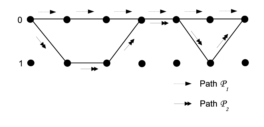
Refer to caption
Fig. 7: Example illustrating the notion of unmerged length between two paths
Definition 1

The unmerged length between the paths 𝒫1\mathcal{P}_{1} and 𝒫2\mathcal{{P}}_{2} in the trellis, denoted as h⁡(𝒫1,𝒫2)h(\mathcal{P}_{1},\mathcal{{P}}_{2}) is the number of branches in which the paths 𝒫1\mathcal{P}_{1} and 𝒫2\mathcal{{P}}_{2} differ. For example, for the paths 𝒫1\mathcal{P}_{1} and 𝒫2\mathcal{P}_{2} of length 6 shown in Fig. 7, the unmerged length h⁡(𝒫1,𝒫2)=5h(\mathcal{P}_{1},\mathcal{{P}}_{2})=5. The unmerged length of the code is the minimum value of h⁡(𝒫1,𝒫2)h(\mathcal{P}_{1},\mathcal{{P}}_{2}), over all possible pairs of paths (𝒫1,𝒫2)(\mathcal{P}_{1},\mathcal{{P}}_{2}) in the trellis.

Note 3

Since the unmerged length between a pair of paths 𝒫1,𝒫2\mathcal{P}_{1},\mathcal{{P}}_{2} is the same in all three trellises 𝒯S1\mathcal{T}_{S_{1}}, 𝒯S2\mathcal{T}_{S_{2}} and 𝒯R\mathcal{T}_{R}, we simply refer to it as the unmerged length in the trellis, without mentioning whether the trellis is 𝒯S1\mathcal{T}_{S_{1}}, 𝒯S2\mathcal{T}_{S_{2}} or 𝒯R\mathcal{T}_{R}.

For two paths 𝒫S\mathcal{P}_{S} and 𝒫~S\mathcal{\tilde{P}}_{S} whose unmerged length is equal to the unmerged length of the code, the first term in the PEP upper bound given by (16) is of diversity order upper bounded by twice the unmerged length of the code, since both |ηs1​(𝒫S,𝒫~S)||\eta_{s_{1}}(\mathcal{P}_{S},\mathcal{\tilde{P}}_{S})| and |ηs1​(𝒫S,𝒫~S)∪ηr​(𝒫S,𝒫~S)||\eta_{s_{1}}(\mathcal{P}_{S},\mathcal{\tilde{P}}_{S})\cup\eta_{r}(\mathcal{P}_{S},\mathcal{\tilde{P}}_{S})| are upper bounded by the unmerged length of the code. Hence, the diversity order of the proposed TCM scheme is upper bounded by twice the unmerged length of the code. The mappings 𝒳S1\mathcal{X}_{S_{1}}, 𝒳S2\mathcal{X}_{S_{2}} and 𝒳R\mathcal{X}_{R} should be chosen such that this bound is met with equality.

For two arbitrary paths 𝒫S\mathcal{P}_{S} and 𝒫~S\mathcal{\tilde{P}}_{S} in the trellis, let the diversity order corresponding to the error event (𝒫S⟶𝒫~𝒮)\left(\mathcal{P}_{S}\longrightarrow\mathcal{\tilde{P}_{S}}\right) be denoted as D⁡(𝒫S,𝒫~𝒮)D(\mathcal{P}_{S},\mathcal{\tilde{P}_{S}}).

Corollary 1

For the proposed TCM scheme, D⁡(𝒫S,𝒫~𝒮)D(\mathcal{P}_{S},\mathcal{\tilde{P}_{S}}) is bounded as,

|ηs1​(𝒫S,𝒫~S)|+|ηs2​(𝒫S,𝒫~S)|≤D⁡(𝒫S,𝒫~𝒮)\displaystyle|\eta_{s_{1}}(\mathcal{P}_{S},\mathcal{\tilde{P}}_{S})|+|\eta_{s_{2}}(\mathcal{P}_{S},\mathcal{\tilde{P}}_{S})|\leq D(\mathcal{P}_{S},\mathcal{\tilde{P}_{S}})
≤min{|ηs1(𝒫S,𝒫~S)|+|ηs2(𝒫s,𝒫~S)∪ηr(𝒫S,𝒫~S)|,\displaystyle\hskip 28.45274pt\leq\min\left\{|\eta_{s_{1}}(\mathcal{P}_{S},\mathcal{\tilde{P}}_{S})|+|\eta_{s_{2}}(\mathcal{P}_{s},\mathcal{\tilde{P}}_{S})\cup\eta_{r}(\mathcal{P}_{S},\mathcal{\tilde{P}}_{S})|,\right.
2|ηs1(𝒫S,𝒫~S)|+|ηs2(𝒫s,𝒫~S)|},\displaystyle\left.\hskip 113.81102pt2|\eta_{s_{1}}(\mathcal{P}_{S},\mathcal{\tilde{P}}_{S})|+|\eta_{s_{2}}(\mathcal{P}_{s},\mathcal{\tilde{P}}_{S})|\right\}, (29)

with equality on both the sides if and only if ηr​(𝒫S,𝒫~S)\eta_{r}(\mathcal{P}_{S},\mathcal{\tilde{P}}_{S}) is a subset of ηs2​(𝒫S,𝒫~S)\eta_{s_{2}}(\mathcal{P}_{S},\mathcal{\tilde{P}}_{S}).

Proof:

From (16), D⁡(𝒫S,𝒫~𝒮)D(\mathcal{P}_{S},\mathcal{\tilde{P}_{S}}) is given by,

D⁡(𝒫S,𝒫~𝒮)\displaystyle D(\mathcal{P}_{S},\mathcal{\tilde{P}_{S}}) =|ηs1(𝒫S,𝒫~S)|+min𝒫R,𝒫~R{|ηs2(𝒫s,𝒫~S)∪ηr(𝒫R,𝒫~R)|\displaystyle=|\eta_{s_{1}}(\mathcal{P}_{S},\mathcal{\tilde{P}}_{S})|+\min_{\mathcal{P}_{R},\mathcal{\tilde{P}}_{R}}\left\{|\eta_{s_{2}}(\mathcal{P}_{s},\mathcal{\tilde{P}}_{S})\cup\eta_{r}(\mathcal{P}_{R},\mathcal{\tilde{P}}_{R})|\right.
+|ηs1(𝒫~R,𝒫~S)∪ηs1(𝒫R,𝒫S)|},\displaystyle\left.\hskip 85.35826pt+|\eta_{s_{1}}(\mathcal{\tilde{P}}_{R},\mathcal{\tilde{P}}_{S})\cup\eta_{s_{1}}(\mathcal{P}_{R},\mathcal{{P}}_{S})|\right\},
≥|ηs1​(𝒫s,𝒫~S)|+min𝒫R,𝒫~R⁡|ηs2​(𝒫s,𝒫~S)∪ηr​(𝒫R,𝒫~R)|\displaystyle\geq|\eta_{s_{1}}(\mathcal{P}_{s},\mathcal{\tilde{P}}_{S})|+\min_{\mathcal{P}_{R},\mathcal{\tilde{P}}_{R}}|\eta_{s_{2}}(\mathcal{P}_{s},\mathcal{\tilde{P}}_{S})\cup\eta_{r}(\mathcal{P}_{R},\mathcal{\tilde{P}}_{R})|
+min𝒫R,𝒫~R⁡|ηs1​(𝒫~R,𝒫~S)∪ηs1​(𝒫R,𝒫S)|.\displaystyle\hskip 56.9055pt+\min_{\mathcal{P}_{R},\mathcal{\tilde{P}}_{R}}|\eta_{s_{1}}(\mathcal{\tilde{P}}_{R},\mathcal{\tilde{P}}_{S})\cup\eta_{s_{1}}(\mathcal{P}_{R},\mathcal{{P}}_{S})|. (30)

The quantity |ηs2​(𝒫s,𝒫~S)∪ηr​(𝒫R,𝒫~R)||\eta_{s_{2}}(\mathcal{P}_{s},\mathcal{\tilde{P}}_{S})\cup\eta_{r}(\mathcal{P}_{R},\mathcal{\tilde{P}}_{R})| attains the minimum value, for the case when 𝒫R=𝒫~R\mathcal{P}_{R}=\mathcal{\tilde{P}}_{R}, in which case ηr​(𝒫R,𝒫~R)\eta_{r}(\mathcal{P}_{R},\mathcal{\tilde{P}}_{R}) is an empty set, or for the case when the set ηr​(𝒫R,𝒫~R)\eta_{r}(\mathcal{P}_{R},\mathcal{\tilde{P}}_{R}) is a subset of ηs2​(𝒫s,𝒫~S)\eta_{s_{2}}(\mathcal{P}_{s},\mathcal{\tilde{P}}_{S}). In both the cases the minimum value attained is |ηs2​(𝒫s,𝒫~S)||\eta_{s_{2}}(\mathcal{P}_{s},\mathcal{\tilde{P}}_{S})|.

The minimum value of |ηs1​(𝒫~R,𝒫~S)∪ηs1​(𝒫R,𝒫S)||\eta_{s_{1}}(\mathcal{\tilde{P}}_{R},\mathcal{\tilde{P}}_{S})\cup\eta_{s_{1}}(\mathcal{P}_{R},\mathcal{{P}}_{S})| equal to zero is attained when 𝒫R=𝒫S\mathcal{P}_{R}=\mathcal{{P}}_{S} and 𝒫~R=𝒫~S\mathcal{\tilde{P}}_{R}=\mathcal{\tilde{P}}_{S}.

Hence from (30) we get the lower bound in (29).

The lower bound in (29) is met with equality if both the minima in (30) are attained for the same choice of the pair (𝒫R,𝒫~R)(\mathcal{P}_{R},\mathcal{\tilde{P}}_{R}), which occurs if and only if 𝒫R=𝒫S\mathcal{P}_{R}=\mathcal{{P}}_{S}, 𝒫~R=𝒫~S\mathcal{\tilde{P}}_{R}=\mathcal{\tilde{P}}_{S} and the the set ηr​(𝒫R,𝒫~R)\eta_{r}(\mathcal{P}_{R},\mathcal{\tilde{P}}_{R}) is a subset of ηs2​(𝒫S,𝒫~S)\eta_{s_{2}}(\mathcal{P}_{S},\mathcal{\tilde{P}}_{S}). In other words, equality in (30) occurs if and only if ηr​(𝒫S,𝒫~S)\eta_{r}(\mathcal{P}_{S},\mathcal{\tilde{P}}_{S}) is a subset of ηs2​(𝒫S,𝒫~S)\eta_{s_{2}}(\mathcal{P}_{S},\mathcal{\tilde{P}}_{S}).

The choice 𝒫R=𝒫S\mathcal{P}_{R}=\mathcal{{P}}_{S} and 𝒫~R=𝒫~S\mathcal{\tilde{P}}_{R}=\mathcal{\tilde{P}}_{S} results in,

|ηs2​(𝒫s,𝒫~S)∪ηr​(𝒫R,𝒫~R)|\displaystyle\left.|\eta_{s_{2}}(\mathcal{P}_{s},\mathcal{\tilde{P}}_{S})\cup\eta_{r}(\mathcal{P}_{R},\mathcal{\tilde{P}}_{R})|\right.
+|ηs1​(𝒫~R,𝒫~S)∪ηs1​(𝒫R,𝒫S)|=|ηs2​(𝒫s,𝒫~S)∪ηr​(𝒫S,𝒫~S)|.\displaystyle\left.\hskip 0.0pt+|\eta_{s_{1}}(\mathcal{\tilde{P}}_{R},\mathcal{\tilde{P}}_{S})\cup\eta_{s_{1}}(\mathcal{P}_{R},\mathcal{{P}}_{S})|\right.=|\eta_{s_{2}}(\mathcal{P}_{s},\mathcal{\tilde{P}}_{S})\cup\eta_{r}(\mathcal{P}_{S},\mathcal{\tilde{P}}_{S})|. (31)

The choice 𝒫R=𝒫~R=𝒫~S\mathcal{P}_{R}=\mathcal{\tilde{P}}_{R}=\mathcal{\tilde{P}}_{S} results in,

|ηs2​(𝒫s,𝒫~S)∪ηr​(𝒫R,𝒫~R)|\displaystyle\left.|\eta_{s_{2}}(\mathcal{P}_{s},\mathcal{\tilde{P}}_{S})\cup\eta_{r}(\mathcal{P}_{R},\mathcal{\tilde{P}}_{R})|\right.
+|ηs1​(𝒫~R,𝒫~S)∪ηs1​(𝒫R,𝒫S)|=|ηs2​(𝒫s,𝒫~S)|+|ηs1​(𝒫S,𝒫~S)|.\displaystyle\left.\hskip 0.0pt+|\eta_{s_{1}}(\mathcal{\tilde{P}}_{R},\mathcal{\tilde{P}}_{S})\cup\eta_{s_{1}}(\mathcal{P}_{R},\mathcal{{P}}_{S})|\right.=|\eta_{s_{2}}(\mathcal{P}_{s},\mathcal{\tilde{P}}_{S})|+|\eta_{s_{1}}(\mathcal{P}_{S},\mathcal{\tilde{P}}_{S})|. (32)

From (31) and (32) we get the upper bound in (29).

Equality in both the lower and upper bounds of (29) occurs if and only if ηr​(𝒫S,𝒫~S)\eta_{r}(\mathcal{P}_{S},\mathcal{\tilde{P}}_{S}) is a subset of ηs2​(𝒫S,𝒫~S)\eta_{s_{2}}(\mathcal{P}_{S},\mathcal{\tilde{P}}_{S}). ∎

Definition 2

The effective length of a pair of paths (𝒫S,𝒫~S)(\mathcal{P}_{S},\mathcal{\tilde{P}}_{S}) in the trellis 𝒯S1\mathcal{T}_{S_{1}} is defined to be the cardinality of the set ηs1​(𝒫S,𝒫~S)\eta_{s_{1}}(\mathcal{P}_{S},\mathcal{\tilde{P}}_{S}). The effective length of the trellis 𝒯S1\mathcal{T}_{S_{1}} is defined to be minimum among the effective lengths of all possible pairs of paths (𝒫S,𝒫~S)(\mathcal{P}_{S},\mathcal{\tilde{P}}_{S}). In a similar way, the effective lengths of the trellises 𝒯S2\mathcal{T}_{S_{2}} and 𝒯R\mathcal{T}_{R} can be defined.

Definition 3

The generalized effective length of a pair of paths (𝒫S,𝒫~S)(\mathcal{P}_{S},\mathcal{\tilde{P}}_{S}) in the trellis pair (𝒯S2,𝒯R)(\mathcal{T}_{S_{2}},\mathcal{T}_{R}) is defined to be the cardinality of the set {ηs2​(𝒫S,𝒫~S)∪ηr​(𝒫S,𝒫~S)}\left\{\eta_{s_{2}}(\mathcal{P}_{S},\mathcal{\tilde{P}}_{S})\cup\eta_{r}(\mathcal{P}_{S},\mathcal{\tilde{P}}_{S})\right\}.

Note 4

If the labellings 𝒳s2\mathcal{X}_{s_{2}} and 𝒳r\mathcal{X}_{r} are the same, the generalized effective length of the pair of paths reduces to the effective length of the pair of paths in the trellis 𝒯S2\mathcal{T}_{S_{2}}, which is equal to the effective length of the pair of paths in the trellis 𝒯R\mathcal{T}_{R}.

If 𝒳s1\mathcal{X}_{s_{1}} and 𝒳s2\mathcal{X}_{s_{2}} are chosen such that the effective lengths of the trellises 𝒯S1\mathcal{T}_{S_{1}} and 𝒯S2\mathcal{T}_{S_{2}} are equal to the unmerged length of the code, then for every pair of paths (𝒫S,𝒫~S)(\mathcal{P}_{S},\mathcal{\tilde{P}}_{S}), |ηs1​(𝒫S,𝒫~S)||\eta_{s_{1}}(\mathcal{P}_{S},\mathcal{\tilde{P}}_{S})| and |ηs2​(𝒫S,𝒫~S)||\eta_{s_{2}}(\mathcal{P}_{S},\mathcal{\tilde{P}}_{S})| are greater than the unmerged length of the code. In that case, from the lower bound in Corollary 1 and from the fact that the diversity order cannot exceed twice the unmerged length of the code, it follows that the diversity order for the proposed scheme is equal to twice the unmerged length of the code. Hence, a sufficient condition to obtain maximum diversity order is to maximize the effective lengths of the trellises 𝒯S1\mathcal{T}_{S_{1}} and 𝒯S2\mathcal{T}_{S_{2}}, independent of the labelling 𝒳r\mathcal{X}_{r}. This is not surprising, since during Phase 2 the source encodes the same bits it encoded and transmitted during Phase 1, maximum diversity order is obtained irrespective of whether the relay transmits during Phase 2 or not. But since σs​d2≪σr​d2\sigma_{sd}^{2}\ll\sigma_{rd}^{2}, from (28) it can be seen that the coding gain is greatly reduced if the relay does not transmit during Phase 2. It is shown in the following subsection that the effective length of 𝒯R\mathcal{T}_{R} also should equal the unmerged length of the code to avoid this reduction in coding gain.

Even though the above condition guarantees maximum diversity, there is no simple expression for D⁡(𝒫S,𝒫~S)D(\mathcal{P}_{S},\mathcal{\tilde{P}}_{S}) (Corollary 1 gives only the upper and lower bounds) and hence it is not clear which error events contribute to the minimum diversity order. Proposition 1 below gives the conditions under which an error event results in the minimum diversity order.

Proposition 1

Assuming that the sufficient condition to obtain full diversity is satisfied, the error event corresponding to a pair of paths contributes to the minimum diversity order if and only if the effective length of the pair of paths in 𝒯S1\mathcal{T}_{S_{1}} and the generalized effective length of the pair of paths in (𝒯S2,𝒯R)(\mathcal{T}_{S_{2}},\mathcal{T}_{R}), are equal to the unmerged length of the code.

Proof:

Let 𝒫S\mathcal{P}_{S} and 𝒫¯S\mathcal{\bar{P}}_{S} be two paths in the trellis. The maps 𝒳S1\mathcal{X}_{S_{1}} and 𝒳S2\mathcal{X}_{S_{2}} are chosen such that the effective lengths of the trellises 𝒯S1\mathcal{T}_{S_{1}} and 𝒯S2\mathcal{T}_{S_{2}} are equal to the unmerged length of the code.

From the lower bound in Corollary 1, D⁡(𝒫S,𝒫¯S)D(\mathcal{P}_{S},\mathcal{\bar{P}}_{S}) is greater than or equal to twice the unmerged length of the code, since |ηs1​(𝒫S,𝒫¯S)||\eta_{s_{1}}(\mathcal{P}_{S},\mathcal{\bar{P}}_{S})| and |ηs2​(𝒫S,𝒫¯S)||\eta_{s_{2}}(\mathcal{P}_{S},\mathcal{\bar{P}}_{S})| are greater than or equal to the unmerged length of the code. Equality can occur only when the set ηr​(𝒫S,𝒫¯S)\eta_{r}(\mathcal{P}_{S},\mathcal{\bar{P}}_{S}) is a subset of ηs2​(𝒫S,𝒫¯S)\eta_{s_{2}}(\mathcal{P}_{S},\mathcal{\bar{P}}_{S}), and the effective lengths of the pair (𝒫S,𝒫¯S)(\mathcal{P}_{S},\mathcal{\bar{P}}_{S}) in both the trellises 𝒯S1\mathcal{T}_{S_{1}} and 𝒯S2\mathcal{T}_{S_{2}}, i.e., |ηs1​(𝒫S,𝒫¯S)||\eta_{s_{1}}(\mathcal{P}_{S},\mathcal{\bar{P}}_{S})| and |ηs2​(𝒫S,𝒫¯S)||\eta_{s_{2}}(\mathcal{P}_{S},\mathcal{\bar{P}}_{S})|, are equal to the unmerged length of the code. Clearly, ηr​(𝒫S,𝒫¯S)\eta_{r}(\mathcal{P}_{S},\mathcal{\bar{P}}_{S}) is not a subset of ηs2​(𝒫S,𝒫¯S)\eta_{s_{2}}(\mathcal{P}_{S},\mathcal{\bar{P}}_{S}), if and only if |ηr​(𝒫S,𝒫¯S)∪ηs2​(𝒫S,𝒫¯S)|⪈|ηs2​(𝒫S,𝒫¯S)||\eta_{r}(\mathcal{P}_{S},\mathcal{\bar{P}}_{S})\cup\eta_{s_{2}}(\mathcal{P}_{S},\mathcal{\bar{P}}_{S})|\gneq|\eta_{s_{2}}(\mathcal{P}_{S},\mathcal{\bar{P}}_{S})|, in which case the generalized effective length of the pair of paths (𝒫S,𝒫¯S)(\mathcal{P}_{S},\mathcal{\bar{P}}_{S}) in the trellis pair (𝒯S2,𝒯R)(\mathcal{T}_{S_{2}},\mathcal{T}_{R}) is greater than unmerged length of the code. Hence, the error event corresponding to a pair of paths give rise to the minimum diversity order, if and only if the conditions given in the statement of the Proposition are satisfied. ∎

In the rest of the paper, it is assumed that the sufficient condition to obtain maximum diversity is satisfied.

For a pair of paths 𝒫S\mathcal{P}_{S} and 𝒫~S\mathcal{\tilde{P}}_{S} resulting in the minimum diversity, only the first term in (16) gives rise to minimum diversity order. Neglecting terms of higher diversity order in (16), we get (28) (shown on the previous to the previous page), where KK is a positive constant.

The criterion to maximize the coding gain is obtained in the following subsection.

IV-C Coding Gain Criterion

Let m1​(𝒫S,𝒫~S)m_{1}(\mathcal{P}_{S},\mathcal{\tilde{P}}_{S}) denote the product distance of the pair of paths (𝒫S,𝒫~S)(\mathcal{P}_{S},\mathcal{\tilde{P}}_{S}) in the trellis 𝒯S1\mathcal{T}_{S_{1}}, i.e.,

m1​(𝒫S,𝒫~S)=∏i∈ηs1​(𝒫S,𝒫~S)|xs1i​(𝒫S)−xs1i​(𝒫~S)|2.\displaystyle m_{1}(\mathcal{P}_{S},\mathcal{\tilde{P}}_{S})=\prod_{i\in\eta_{s_{1}}(\mathcal{P}_{S},\mathcal{\tilde{P}}_{S})}{\left|x_{s_{1}}^{i}\left(\mathcal{P}_{S}\right)-x_{s_{1}}^{i}(\mathcal{\tilde{P}}_{S})\right|^{2}}.
Definition 4

The generalized product distance of the pair of paths (𝒫S,𝒫~S)(\mathcal{P}_{S},\mathcal{\tilde{P}}_{S}) corresponding to the trellis pair (𝒯S2,𝒯R)(\mathcal{T}_{S_{2}},\mathcal{T}_{R}) denoted as m2​(𝒫S,𝒫~S)m_{2}(\mathcal{P}_{S},\mathcal{\tilde{P}}_{S}) is defined as,

m2(𝒫S,𝒫~S)=∏i∈{ηs2​(𝒫S,𝒫~S)∪ηr​(𝒫S,𝒫~S)}(γ|xs2i(𝒫S)−xs2i(𝒫~S)|2)\displaystyle m_{2}(\mathcal{P}_{S},\mathcal{\tilde{P}}_{S})=\prod_{i\in\left\{\eta_{s_{2}}(\mathcal{P}_{S},\mathcal{\tilde{P}}_{S})\cup\eta_{r}(\mathcal{P}_{S},\mathcal{\tilde{P}}_{S})\right\}}\left(\gamma\left|x_{s_{2}}^{i}\left(\mathcal{P}_{S}\right)-x_{s_{2}}^{i}(\mathcal{\tilde{P}}_{S})\right|^{2}\hskip 2845.27559pt\right)
(+|xri​(𝒫S)−xri​(𝒫~S)|2),\displaystyle\hskip-569.05511pt\left(\hskip 711.3189pt+\left|x_{r}^{i}\left(\mathcal{P}_{S}\right)-{x}_{r}^{i}(\mathcal{\tilde{P}}_{S})\right|^{2}\right), (33)

where γ=σs​d2/σr​d2\gamma=\sigma_{sd}^{2}/\sigma_{rd}^{2}.

Note 5

If the labelling used for the trellises 𝒯R\mathcal{T}_{R} and 𝒯S2\mathcal{T}_{S_{2}} are the same, the generalized product distance of the pair of paths (𝒫S,𝒫~S)(\mathcal{P}_{S},\mathcal{\tilde{P}}_{S}) corresponding to the trellis pair (𝒯S2,𝒯R)(\mathcal{T}_{S_{2}},\mathcal{T}_{R}), reduces within a constant scaling factor to the product distance of the pair of paths (𝒫S,𝒫~S)(\mathcal{P}_{S},\mathcal{\tilde{P}}_{S}) in the trellis 𝒯R\mathcal{T}_{R}, which is equal to the product distance of the pair of paths (𝒫S,𝒫~S)(\mathcal{P}_{S},\mathcal{\tilde{P}}_{S}) in the trellis 𝒯S2\mathcal{T}_{S_{2}}.

Definition 5

Consider the trellis triplet (𝒯S1,𝒯S2,𝒯R)(\mathcal{T}_{S_{1}},\mathcal{T}_{S_{2}},\mathcal{T}_{R}). The combined product distance of the pair of paths (𝒫S,𝒫~S)(\mathcal{P}_{S},\mathcal{\tilde{P}}_{S}), denoted by m⁡(𝒫S,𝒫~S)m(\mathcal{P}_{S},\mathcal{\tilde{P}}_{S}), is defined as the product of the product distance of the pair of paths (𝒫S,𝒫~S)(\mathcal{P}_{S},\mathcal{\tilde{P}}_{S}) in the trellis 𝒯S1\mathcal{T}_{S_{1}} and the generalised product distance of the pair of paths (𝒫S,𝒫~S)(\mathcal{P}_{S},\mathcal{\tilde{P}}_{S}) corresponding to the trellis pair (𝒯S2,𝒯R)(\mathcal{T}_{S_{2}},\mathcal{T}_{R}), i.e.,

m⁡(𝒫S,𝒫~S)=[m1​(𝒫S,𝒫~S)​m2​(𝒫S,𝒫~S)].\displaystyle{m(\mathcal{P}_{S},\mathcal{\tilde{P}}_{S})}=\left[m_{1}(\mathcal{P}_{S},\mathcal{\tilde{P}}_{S})m_{2}(\mathcal{P}_{S},\mathcal{\tilde{P}}_{S})\right].
Definition 6

The combined product distance of the trellis triplet (𝒯S1,𝒯S2,𝒯R)(\mathcal{T}_{S_{1}},\mathcal{T}_{S_{2}},\mathcal{T}_{R}), which is also the coding gain metric denoted by 𝒢\mathcal{G}, is defined to be the minimum value of m⁡(𝒫S,𝒫~S)m(\mathcal{P}_{S},\mathcal{\tilde{P}}_{S}), i.e.,

𝒢=min(𝒫S,𝒫~S)∈𝒵𝒫⁡[m⁡(𝒫S,𝒫~S)].\displaystyle\mathcal{G}=\min_{(\mathcal{P}_{S},\mathcal{\tilde{P}}_{S})\in\mathcal{Z_{P}}}\left[m(\mathcal{P}_{S},\mathcal{\tilde{P}}_{S})\right].

where 𝒵𝒫\mathcal{Z_{P}} denotes the set of all pairs of paths (𝒫S,𝒫~S)(\mathcal{P}_{S},\mathcal{\tilde{P}}_{S}) whose effective length in 𝒯S1\mathcal{T}_{S_{1}} and the generalized effective length in (𝒯S2,𝒯R)(\mathcal{T}_{S_{2}},\mathcal{T}_{R}) are equal to the unmerged length of the code.

From (28), it can be seen that the combined product distance of the trellis triplet (𝒯S1,𝒯S2,𝒯R)(\mathcal{T}_{S_{1}},\mathcal{T}_{S_{2}},\mathcal{T}_{R}) needs to be maximized, to maximize the coding gain. For a pair of paths (𝒫S,𝒫~S)(\mathcal{P}_{S},\mathcal{\tilde{P}}_{S}) which contribute to the minimum diversity order, if the effective length of (𝒫S,𝒫~S)(\mathcal{P}_{S},\mathcal{\tilde{P}}_{S}) in the trellis 𝒯R\mathcal{T}_{R} is not equal to the unmerged length of the code, then xri​(𝒫S)=xri​(𝒫~S)x_{r}^{i}(\mathcal{P}_{S})=x_{r}^{i}(\mathcal{\tilde{P}}_{S}) for some i∈ηr​(𝒫S,𝒫~S)i\in\eta_{r}(\mathcal{P}_{S},\mathcal{\tilde{P}}_{S}). In that case m2​(𝒫S,𝒫~S)m_{2}(\mathcal{P}_{S},\mathcal{\tilde{P}}_{S}) is greatly reduced since γ≪1\gamma\ll 1. In order to avoid this, the effective length of the trellis 𝒯R\mathcal{T}_{R} should be made equal to the unmerged length of the code.

IV-D Near Optimality of the Proposed Near-ML decoder

Pr{𝒫S⟶𝒫~S}≤exp{∑i=1L(−12|hs​d1i(xs1i(𝒫S)−(xs1i(𝒫~S))|2−12|hs​d2i(xs2i(𝒫S)−(xs2i(𝒫~S))+hr​di(xri(𝒫S)−xri(𝒫~S))|2)}\displaystyle Pr\left\{\mathcal{P}_{S}\longrightarrow{\mathcal{\tilde{P}}_{S}}\right\}\leq\exp\left\{\sum_{i=1}^{L}\left(-\dfrac{1}{2}\left|h_{sd_{1}}^{i}\left(x_{s_{1}}^{i}\left(\mathcal{P}_{S}\right)-(x_{s_{1}}^{i}(\mathcal{\tilde{P}}_{S})\right)\right|^{2}-\dfrac{1}{2}\left|h_{sd_{2}}^{i}\left(x_{s_{2}}^{i}\left(\mathcal{P}_{S}\right)-(x_{s_{2}}^{i}(\mathcal{\tilde{P}}_{S})\right)+h_{rd}^{i}\left(x_{r}^{i}\left(\mathcal{P}_{S}\right)-{x}_{r}^{i}(\mathcal{\tilde{P}}_{S})\right)\right|^{2}\right)\right\} (34)
P​r​(𝒫S⟶𝒫~𝒮)≤K​∏i∈ηs1​(𝒫S,𝒫~S)[1|σs​d(xs1i(𝒫S)−(xs1i(𝒫~S))|2]\displaystyle Pr\left(\mathcal{P}_{S}\longrightarrow\mathcal{\tilde{P}_{S}}\right)\leq{K}\prod_{i\in\eta_{s_{1}}(\mathcal{P}_{S},\mathcal{\tilde{P}}_{S})}\left[\dfrac{1}{{\left|\sigma_{sd}\left(x_{s_{1}}^{i}\left(\mathcal{P}_{S}\right)-(x_{s_{1}}^{i}(\mathcal{\tilde{P}}_{S})\right)\right|^{2}}}\right]
∏i∈{ηs2​(𝒫S,𝒫~S)∪ηr​(𝒫S,𝒫~S)}[1|σs​d(xs2i(𝒫S)−(xs2i(𝒫~S))|2+|σr​d(xri(𝒫S)−xri(𝒫~S))|2]\displaystyle\hskip 142.26378pt\prod_{i\in\left\{\eta_{s_{2}}(\mathcal{P}_{S},\mathcal{\tilde{P}}_{S})\cup\eta_{r}(\mathcal{P}_{S},\mathcal{\tilde{P}}_{S})\right\}}\left[\dfrac{1}{{\left|\sigma_{sd}\left(x_{s_{2}}^{i}\left(\mathcal{P}_{S}\right)-(x_{s_{2}}^{i}(\mathcal{\tilde{P}}_{S})\right)\right|^{2}+\left|\sigma_{rd}\left(x_{r}^{i}\left(\mathcal{P}_{S}\right)-{x}_{r}^{i}(\mathcal{\tilde{P}}_{S})\right)\right|^{2}}}\right] (35)


The following argument proves the high SNR near optimality of the proposed near-ML decoder for the TCM scheme. Consider the situation where the S-R link is ideal, i.e., the relay decodes all the bits correctly. The optimal ML decoder at D decides in favour of the path given by,

𝒫^S\displaystyle\mathcal{\hat{P}}_{S} =arg⁡min𝒫S∈𝒜L⁡(∑i=1L|Yd1i−hs​d1i​xs1i​(𝒫S)|2CLOSE\displaystyle=\arg\min_{\mathcal{P}_{S}\in\mathcal{A}_{L}}\left(\sum_{i=1}^{L}\left|Y_{d_{1}}^{i}-h_{sd_{1}}^{i}x_{s_{1}}^{i}\left(\mathcal{P}_{S}\right)\right|^{2}\right.
OPEN+|Yd2i−hs​d2i​xs2i​(𝒫S)−hr​di​xri​(𝒫S)|2).\displaystyle\hskip 71.13188pt\left.+\left|Y_{d_{2}}^{i}-h_{sd_{2}}^{i}x_{s_{2}}^{i}\left(\mathcal{P}_{S}\right)-h_{rd}^{i}x_{r}^{i}\left(\mathcal{P}_{S}\right)\right|^{2}\right).

For this case, the PEP that the path 𝒫S\mathcal{P}_{S} is decoded as 𝒫~S\mathcal{\tilde{P}}_{S} is upper bounded by (34) (shown at the top of the next page). Taking expectation with respect to the fading coefficients, we get (35) (shown at the top of the next page). From (28) and (35), we see that the high SNR bounds on the PEP for the proposed near ML decoder with a non-ideal S-R link is same as that of the optimal ML decoder with an ideal S-R link, if we consider only the error events giving rise to the minimum diversity order. The simulation results presented in Section VII confirm that the BER vs SNR performance of the proposed near ML decoder with a non-ideal S-R link approaches the performance of optimal ML decoder with an ideal S-R link, at high SNR. The high SNR performance of the optimal ML decoder for the proposed TCM scheme, with a non-ideal S-R link cannot be better than that of optimal ML decoder for the case when the S-R link is ideal. This implies the high SNR performance of the proposed near-ML decoder approaches the performance of the optimal ML decoder.

From (28), it is clearly seen that even for the uncoded transmission scheme, choosing the labelling schemes used at S and R properly can potentially yield a significant performance improvement. The effect of the choice of labelling on the performance for the uncoded transmission scheme is discussed in the following section.

V THE UNCODED TRANSMISSION SCHEME

Consider the uncoded transmission scheme in which bits are directly mapped onto complex symbols at S and R. A collection of l​o​g2​Mlog_{2}M bits constitutes a message. Let ℳ={1,2,…,M}\mathcal{M}=\{1,2,...,M\} denote this message set. The uncoded transmission scheme has an equivalent one state trellis representation, with MM edges connecting two successive stages. The unmerged length between every pair of distinct paths is one and hence no distinction needs to be made between paths and edges. The index ii in the transmitted complex numbers xs1i(.)x_{s_{1}}^{i}(.), xs2i(.)x_{s_{2}}^{i}(.) and xri(.)x_{r}^{i}(.) can be dropped and they are the same as the labellings on the edges 𝒳s1(.)\mathcal{X}_{s_{1}}(.), 𝒳s2(.)\mathcal{X}_{s_{2}}(.) and 𝒳r(.)\mathcal{X}_{r}(.). Each path (edge) in the trellis is identified by the message a∈ℳa\in\mathcal{M} which gets transmitted.

Corollary 2

For the uncoded transmission scheme, the PEP that the decoder at D decides in favour of message a¯∈ℳ\bar{a}\in\mathcal{M} given that the message transmitted by the source was a∈ℳa\in\mathcal{M} is upper bounded as,

P​r​(a⟶a¯)≤\displaystyle Pr\left(a\longrightarrow\bar{a}\right)\leq
[11+14​|σs​d|2​|xs1​(a)−xs1​(a¯)|2]\displaystyle\hskip 0.0pt\left[\dfrac{1}{1+\dfrac{1}{4}|\sigma_{sd}|^{2}|x_{s_{1}}({a})-x_{s_{1}}(\bar{a})|^{2}}\right]
[11+14​|σs​d|2​|xs2​(a)−xs2​(a¯)|2+14​|σr​d|2​|xr​(a)−xr​(a¯)|2]\displaystyle\left[\dfrac{1}{1+\dfrac{1}{4}|\sigma_{sd}|^{2}|x_{s_{2}}({a})-x_{s_{2}}(\bar{a})|^{2}+\dfrac{1}{4}|\sigma_{rd}|^{2}|x_{r}({a})-x_{r}(\bar{a})|^{2}}\right]
+H.O.T.\displaystyle\hskip 219.08612pt+H.O.T.

where H.O.T denotes the terms of diversity order greater than 2.

Proof:

From (16), replacing the paths 𝒫S\mathcal{P}_{S}, 𝒫~S\mathcal{\tilde{P}}_{S}, 𝒫R\mathcal{P}_{R} and 𝒫~R\mathcal{\tilde{P}}_{R} by the corresponding message indices, we get (36) (shown at the top of the next page). Neglecting terms of diversity order greater than 2 gives the result. ∎

Pr(a⟶a¯)≤∑l=1M([11+|σd​s​(xs1​(a)−xs1​(a¯))|24][11+|σd​s​(xs2​(a)−xs2​(a¯))|24+|σd​r​(xr​(a)−xr​(l))|24])\displaystyle Pr(a\longrightarrow\bar{a})\leq\sum_{l=1}^{M}\left(\left[\dfrac{1}{1+\dfrac{|\sigma_{ds}\left(x_{s_{1}}\left(a\right)-x_{s_{1}}\left(\bar{a}\right)\right)|^{2}}{4}}\right]\left[\dfrac{1}{1+\dfrac{|\sigma_{ds}\left(x_{s_{2}}\left(a\right)-x_{s_{2}}\left(\bar{a}\right)\right)|^{2}}{4}+\dfrac{|\sigma_{dr}\left(x_{r}\left(a\right)-x_{r}\left({l}\right)\right)|^{2}}{4}}\right]\hskip 853.58267pt\right)
([11+|σr​s​(xs1​(a¯)−xs1​(l))|28])\displaystyle\hskip-426.79134pt\left(\hskip 790.9867pt\left[\dfrac{1}{1+\dfrac{|\sigma_{rs}\left(x_{s_{1}}\left(\bar{a}\right)-x_{s_{1}}\left(l\right)\right)|^{2}}{8}}\right]\hskip 0.0pt\right)
+∑j=1,j≠aM∑m=1M([11+|σd​s​(xs1​(a)−xs1​(a¯))|24][11+|σd​s​(xs2​(a)−xs2​(a¯))|24+|σd​r​(xr​(j)−xr​(m))|24])\displaystyle\hskip 56.9055pt+\sum_{j=1,j\neq a}^{M}\sum_{m=1}^{M}\left(\left[\dfrac{1}{1+\dfrac{|\sigma_{ds}\left(x_{s_{1}}\left(a\right)-x_{s_{1}}\left(\bar{a}\right)\right)|^{2}}{4}}\right]\left[\dfrac{1}{1+\dfrac{|\sigma_{ds}\left(x_{s_{2}}\left(a\right)-x_{s_{2}}\left(\bar{a}\right)\right)|^{2}}{4}+\dfrac{|\sigma_{dr}\left(x_{r}\left(j\right)-x_{r}\left({m}\right)\right)|^{2}}{4}}\right]\hskip 853.58267pt\right)
([11+|σr​s​(xs1​(a)−xs1​(j))|28+|σr​s​(xs1​(a¯)−xs1​(m))|28])\displaystyle\hskip-569.05511pt\left(\hskip 825.12991pt\left[\dfrac{1}{1+\dfrac{|\sigma_{rs}\left(x_{s_{1}}\left({a}\right)-x_{s_{1}}\left(j\right)\right)|^{2}}{8}+\dfrac{|\sigma_{rs}\left(x_{s_{1}}\left(\bar{a}\right)-x_{s_{1}}\left(m\right)\right)|^{2}}{8}}\right]\right) (36)


From Corollary 2, it follows that the diversity order of the uncoded transmission scheme is two and in order to minimise the PEP, we need to maximize the following:

[1+14​|σs​d|2​|xs1​(a)−xs1​(a¯)|2]\displaystyle\hskip 0.0pt\left[{1+\dfrac{1}{4}|\sigma_{sd}|^{2}|x_{s_{1}}({a})-x_{s_{1}}(\bar{a})|^{2}}\right]
[1+14​|σs​d|2​|xs2​(a)−xs2​(a¯)|2+14​|σr​d|2​|xr​(a)−xr​(a¯)|2].\displaystyle\left[{1+\dfrac{1}{4}|\sigma_{sd}|^{2}|x_{s_{2}}({a})-x_{s_{2}}(\bar{a})|^{2}+\dfrac{1}{4}|\sigma_{rd}|^{2}|x_{r}({a})-x_{r}(\bar{a})|^{2}}\right].

At high SNR we need to maximize the metric,

m⁡(a,a¯)=\displaystyle m(a,\bar{a})= |xs1​(a)−xs1​(a¯)|2\displaystyle{|x_{s_{1}}({a})-x_{s_{1}}(\bar{a})|^{2}}
[γ​|xs2​(a)−xs2​(a¯)|2+|xr​(a)−xr​(a¯)|2],\displaystyle\left[{\gamma|x_{s_{2}}({a})-x_{s_{2}}(\bar{a})|^{2}+|x_{r}({a})-x_{r}(\bar{a})|^{2}}\right],

over all message pairs (a,a¯)(a,\bar{a}).

By a labelling scheme, we refer to the triplet (𝒳s1,𝒳s2,𝒳r)(\mathcal{X}_{s_{1}},\mathcal{X}_{s_{2}},\mathcal{X}_{r}). Let ℒ\mathcal{L} denote a labelling scheme used at S and R. Let us define,

d⁡(ℒ)\displaystyle d(\mathcal{L}) =mina,a¯,a≠a¯⁡m⁡(a,a¯),\displaystyle=\min_{a,\bar{a},a\neq\bar{a}}m(a,\bar{a}),

where a,a¯∈ℳa,\bar{a}\in\mathcal{M}.

Let ℒ0\mathcal{L}_{0} denote the labelling scheme in which the mapping from bits to complex symbols, used by S (during Phase 1 and Phase 2) and R (during Phase 2), are the same. Similar to d⁡(ℒ)d(\mathcal{L}), d⁡(ℒ0)d(\mathcal{L}_{0}) can be defined for the labelling scheme ℒ0\mathcal{L}_{0}.

Definition 7

The Labelling Gain of the labelling scheme ℒ\mathcal{L}, which is a measure of the performance gain provided by ℒ\mathcal{L} over ℒ0\mathcal{L}_{0}, is given by,
LG​(ℒ)=10​log10​[d⁡(ℒ)d⁡(ℒ0)]L_{G}(\mathcal{L})=10\log_{10}\left[{\dfrac{d(\mathcal{L})}{d(\mathcal{L}_{0})}}\right] dB.

It is important to note that the Labelling Gain is calculated based on the upper bound on the PEP, taking into consideration only those pair of messages aa and a¯\bar{a} which contribute dominantly to the metric m⁡(a,a¯)m(a,\bar{a}). The actual high SNR gain provided by the labelling scheme ℒ\mathcal{L} over the scheme ℒ0\mathcal{L}_{0} need not equal LG​(ℒ)L_{G}(\mathcal{L}).

Throughout, the phrase with our labelling means that S and R use the labelling scheme which is described in the following subsection and with constant labelling means that S and R use the labelling scheme ℒ0\mathcal{L}_{0}.

V-A A Labelling Scheme for PSK Constellation

In this subsection, we provide a good labelling scheme for 2l2^{l}-PSK constellation, where l≥2l\geq 2 is an integer. Let sk=exp⁡(j​k​2​π/M)s_{k}=\exp{\left(jk2\pi/M\right)}, where 0≤k≤M−10\leq k\leq M-1 and M=2lM=2^{l}, denote the signal points in the 2l2^{l}-PSK signal set.

Let ℒ¯\mathcal{\bar{L}} denote the labelling scheme described as follows: The maps 𝒳s1\mathcal{X}_{s_{1}}, 𝒳r\mathcal{X}_{r} and 𝒳s2\mathcal{X}_{s_{2}} are given by,

𝒳s1​(k)=sk,\displaystyle\mathcal{X}_{s_{1}}(k)=s_{k},
𝒳r​(k)={sk,if​k​is​even,s(k+M/2modM),if​k​is​odd,\displaystyle\mathcal{X}_{r}(k)=\left\{\begin{array}[]{ll}s_{k},&\>\mathrm{if}\>k\>\mathrm{is}\>\mathrm{even},\\ s_{(k+M/2\mod M)},&\>\mathrm{if}\>k\>\mathrm{is}\>\mathrm{odd},\\ \end{array}\right.
𝒳s2​(k)=sk,\displaystyle\mathcal{X}_{s_{2}}(k)=s_{k},

where 0≤k≤M−10\leq k\leq M-1.

Theorem 2

For the labelling scheme ℒ¯\mathcal{\bar{L}}, with 2l2^{l}-PSK signal set, the labelling gain, assuming γ≪1\gamma\ll 1, is approximately given by,

LG​(ℒ¯)\displaystyle{L}_{G}(\mathcal{\bar{L}}) ≈{20​log10​[cot⁡(π/2l)],for​l=2,3;20​log10​[4​cos2⁡(π/2l)],for​l≥4.\displaystyle\approx\left\{\begin{array}[]{ll}&20\log_{10}\left[\cot(\pi/2^{l})\right],\>\mathrm{for}\>l=2,3;\\ &20\log_{10}\left[4\cos^{2}(\pi/2^{l})\right],\>\mathrm{for}\>l\geq 4.\\ \end{array}\right.
Proof:

Let us define,

d1​(k,k′)\displaystyle d_{1}(k,k^{\prime}) =|𝒳s1​(k)−𝒳s1​(k′)|\displaystyle=|\mathcal{X}_{s_{1}}(k)-\mathcal{X}_{s_{1}}(k^{\prime})|
=|exp⁡(j​k​2​π/M)−exp⁡(j​k′​2​π/M)|\displaystyle=|\exp(jk2\pi/M)-\exp(jk^{\prime}2\pi/M)|
=|1−exp⁡(j⁡(k′−k)​2​π/M)|,\displaystyle=|1-\exp(j(k^{\prime}-k)2\pi/M)|,

where 0≤k,k′≤M−10\leq k,k^{\prime}\leq M-1.

Since d1​(k,k′)d_{1}(k,k^{\prime}) depends only on |k−k′||k-k^{\prime}|, let us denote it by d1​(n)d_{1}(n), where 0≤|k−k′|=n≤M0\leq|k-k^{\prime}|=n\leq M . Then,

d1​(n)\displaystyle d_{1}(n) =|1−exp⁡(j​n​2​π/M)|\displaystyle=|1-\exp(jn2\pi/M)|
=2​|sin⁡(π​n/M)|,\displaystyle=2|\sin(\pi n/M)|, (38)

where 0≤n≤M0\leq n\leq M. Similarly, let us define,

d2​(n)\displaystyle d_{2}(n) =|𝒳r​(k)−𝒳r​(k′)|\displaystyle=|\mathcal{X}_{r}(k)-\mathcal{X}_{r}(k^{\prime})|
={|1−exp⁡(j​n​2​π/M)|,for​n​even|1+exp⁡(j​n​2​π/M)|,for​n​odd\displaystyle=\left\{\begin{array}[]{ll}&|1-\exp(jn2\pi/M)|,\>\mathrm{for}\>n\>\mathrm{even}\\ &|1+\exp(jn2\pi/M)|,\>\mathrm{for}\>n\>\mathrm{odd}\\ \end{array}\right.
={2​|sin⁡(π​n/M)|,for​n​even2​|cos⁡(π​n/M)|,for​n​odd.\displaystyle=\left\{\begin{array}[]{ll}&2|\sin(\pi n/M)|,\>\mathrm{for}\>n\>\mathrm{even}\\ &2|\cos(\pi n/M)|,\>\mathrm{for}\>n\>\mathrm{odd}\\ \end{array}\right..

Since γ≪1\gamma\ll 1, we have

d⁡(ℒ¯)\displaystyle d(\mathcal{\bar{L}}) ≈mink≠k′⁡|𝒳s1​(k)−𝒳s1​(k′)|2​|𝒳r​(k)−𝒳r​(k′)|2\displaystyle\approx\min_{k\neq k^{\prime}}|\mathcal{X}_{s_{1}}({k})-\mathcal{X}_{s_{1}}(k^{\prime})|^{2}|\mathcal{X}_{r}({k})-\mathcal{X}_{r}({k^{\prime}})|^{2}
=min1≤n≤M⁡d12​(n)​d22​(n)\displaystyle=\min_{1\leq n\leq M}d_{1}^{2}(n)d_{2}^{2}(n)
=min1≤n≤M⁡(minn​even⁡[d12​(n)​d22​(n)],minn​odd⁡[d12​(n)​d22​(n)]).\displaystyle=\min_{1\leq n\leq M}(\min_{n\>\textrm{even}}[d_{1}^{2}(n)d_{2}^{2}(n)],\min_{n\>\textrm{odd}}[d_{1}^{2}(n)d_{2}^{2}(n)]). (42)

From (38) and (2) we have,

min1≤n≤Mn​even⁡[d12​(n)​d22​(n)]\displaystyle\min_{\begin{subarray}{c}{1\leq n\leq M}\\ {n\>\textrm{even}}\end{subarray}}[d_{1}^{2}(n)d_{2}^{2}(n)] =min1≤n≤Mn​even⁡[16​sin4⁡(π​n/M)]\displaystyle=\min_{\begin{subarray}{c}{1\leq n\leq M}\\ {n\>\textrm{even}}\end{subarray}}[16\sin^{4}(\pi n/M)]
=16​sin4⁡(2​π/M)\displaystyle=16\sin^{4}(2\pi/M) (43)

and similarly,

min1≤n≤Mn​odd⁡[d12​(n)​d22​(n)]\displaystyle\min_{\begin{subarray}{c}{1\leq n\leq M}\\ {n\>\textrm{odd}}\end{subarray}}[d_{1}^{2}(n)d_{2}^{2}(n)] =min1≤n≤Mn​odd⁡[16​sin2⁡(π​n/M)​cos2⁡(π​n/M)]\displaystyle=\min_{\begin{subarray}{c}{1\leq n\leq M}\\ {n\>\textrm{odd}}\end{subarray}}[16\sin^{2}(\pi n/M)\cos^{2}(\pi n/M)]
=4​sin2⁡(2​π/M).\displaystyle=4\sin^{2}(2\pi/M). (44)

Substituting (43) and (44) in (42) we have,

d⁡(ℒ¯)\displaystyle d(\mathcal{\bar{L}}) ≈min⁡[16​sin4⁡(2​π/M),4​sin2⁡(2​π/M)].\displaystyle\approx\min[16\sin^{4}(2\pi/M),4\sin^{2}(2\pi/M)]. (45)

Also, we have

d⁡(ℒ0)\displaystyle d(\mathcal{{L}}_{0}) ≈min1≤n≤M⁡d14​(n)\displaystyle\approx\min_{1\leq n\leq M}d_{1}^{4}(n)
=16​sin4⁡(π/M).\displaystyle=16\sin^{4}(\pi/M). (46)

Hence, from (45) and (46), by definition of LG​(ℒ¯){L}_{G}(\mathcal{\bar{L}}), we have,

LG​(ℒ¯)=20​log10​[min⁡(cot⁡(π/M),4​cos2⁡(π/M))].\displaystyle{L}_{G}(\mathcal{\bar{L}})=20\log_{10}[\min(\cot(\pi/M),4\cos^{2}(\pi/M))].

It can be verified that cot⁡(π/M)⪈4​cos2⁡(π/M)\cot(\pi/M)\gneq 4\cos^{2}(\pi/M) for M⪈12M\gneq 12, from which we get (). ∎

It can be seen from Theorem 2 that for l=2l=2, the labelling gain LG​(ℒ¯)≈0{L}_{G}(\mathcal{\bar{L}})\approx 0 dB. In other words, for the uncoded transmission scheme using 4 PSK, using different labelling schemes at S and R does not provide any performance improvement. It can be seen that cot⁡(π/2l)\cot(\pi/2^{l}) for l=3l=3, and 4​cos2⁡(π/2l)4\cos^{2}(\pi/2^{l}) for l≥4l\geq 4 are greater than one, whence the approximate value of LG​(ℒ¯){L}_{G}(\mathcal{\bar{L}}) is greater than 0 dB for l≥3l\geq 3. Since LG​(ℒ¯){L}_{G}(\mathcal{\bar{L}}) is always greater than the approximate value given by Theorem 2, for the uncoded transmission scheme using 2l2^{l} PSK, using our labelling scheme provides advantage over constant labelling, for all l≥3l\geq 3. Furthermore, since 4​cos2⁡(π/2l)4\cos^{2}(\pi/2^{l}) is an increasing function of ll, the labelling gain increases with increasing size of the PSK constellation. Simulation results presented in Section VII confirm that the uncoded transmission with our labelling outperforms the uncoded transmission with constant labelling.

VI TCM CODE DESIGN GUIDELINES AND EXAMPLES

VI-A TCM Code Design Guidelines

Let the generalized product distance m2​(𝒫S,𝒫~S)m_{2}(\mathcal{P}_{S},\mathcal{\tilde{P}}_{S}) be split into two parts as,

m2​(𝒫S,𝒫~S)=m21​(𝒫S,𝒫~S)+m22​(𝒫S,𝒫~S),\displaystyle m_{2}(\mathcal{P}_{S},\mathcal{\tilde{P}}_{S})=m_{21}(\mathcal{P}_{S},\mathcal{\tilde{P}}_{S})+m_{22}(\mathcal{P}_{S},\mathcal{\tilde{P}}_{S}),

where the product distances m21​(𝒫S,𝒫~S)m_{21}(\mathcal{P}_{S},\mathcal{\tilde{P}}_{S}) and m22​(𝒫S,𝒫~S)m_{22}(\mathcal{P}_{S},\mathcal{\tilde{P}}_{S}) are given by,

m21​(𝒫S,𝒫~S)=∏i∈η2​(𝒫S,𝒫~S)|xri​(𝒫S)−xri​(𝒫~S)|2,\displaystyle m_{21}(\mathcal{P}_{S},\mathcal{\tilde{P}}_{S})=\prod_{i\in\eta_{2}(\mathcal{P}_{S},\mathcal{\tilde{P}}_{S})}\left|x_{r}^{i}\left(\mathcal{P}_{S}\right)-{x}_{r}^{i}(\mathcal{\tilde{P}}_{S})\right|^{2},
m22​(𝒫S,𝒫~S)=∏i∈η2​(𝒫S,𝒫~S)γ​|xs2i​(𝒫S)−xs2i​(𝒫~S)|2.\displaystyle m_{22}(\mathcal{P}_{S},\mathcal{\tilde{P}}_{S})=\prod_{i\in\eta_{2}(\mathcal{P}_{S},\mathcal{\tilde{P}}_{S})}\gamma\left|x_{s_{2}}^{i}\left(\mathcal{P}_{S}\right)-x_{s_{2}}^{i}(\mathcal{\tilde{P}}_{S})\right|^{2}.

Let 𝒢1\mathcal{G}_{1} and 𝒢2\mathcal{G}_{2} be two metrics defined as,

𝒢1=min(𝒫S,𝒫~S)∈𝒴𝒫⁡[m1​(𝒫S,𝒫~S)],\displaystyle\mathcal{G}_{1}=\min_{(\mathcal{P}_{S},\mathcal{\tilde{P}}_{S})\in\mathcal{Y_{P}}}\left[m_{1}(\mathcal{P}_{S},\mathcal{\tilde{P}}_{S})\right],
𝒢2=min(𝒫S,𝒫~S)∈𝒵𝒫⁡[m1​(𝒫S,𝒫~S)​m21​(𝒫S,𝒫~S)],\displaystyle\mathcal{G}_{2}=\min_{(\mathcal{P}_{S},\mathcal{\tilde{P}}_{S})\in\mathcal{Z_{P}}}\left[m_{1}(\mathcal{P}_{S},\mathcal{\tilde{P}}_{S})m_{21}(\mathcal{P}_{S},\mathcal{\tilde{P}}_{S})\right],

where 𝒴𝒫\mathcal{Y_{P}} denotes the set of pairs of paths whose effective length is equal to the effective length of the trellis 𝒯S1\mathcal{T}_{S_{1}}.

The code design guidelines are summarized below. Some of the design rules for TCM for the point to point AWGN and fading channels ([20],[21]), carry over for the relay channel as well.

  • •

    Since trellises with parallel transitions limit the effective length of the trellis to one, they should be avoided.

  • •

    Signal points from the signal set should occur with equal frequency.

  • •

    In a trellis with regularity and symmetry, two branches which emerge from the same state form a part of a pair of paths which differ by a unmerged length equal to the unmerged length of the code. Since the coding gain metric 𝒢\mathcal{G} involves parameters m1​(𝒫S,𝒫~S)m_{1}(\mathcal{P}_{S},\mathcal{\tilde{P}}_{S}), m21​(𝒫S,𝒫~S)m_{21}(\mathcal{P}_{S},\mathcal{\tilde{P}}_{S}) and m22​(𝒫S,𝒫~S)m_{22}(\mathcal{P}_{S},\mathcal{\tilde{P}}_{S}), which are of the form of product of the branch Euclidean distances of the pair of paths (𝒫S,𝒫~S)(\mathcal{P}_{S},\mathcal{\tilde{P}}_{S}), signal points assigned to branches emerging from the same state should be from the same Ungerboeck partition [20].

Since γ≪1\gamma\ll 1, the values of 𝒢\mathcal{G} and 𝒢2\mathcal{G}_{2} are nearly equal and instead of maximizing 𝒢\mathcal{G}, 𝒢2\mathcal{G}_{2} can be maximized. In the design examples presented, the choice of 𝒳s1\mathcal{X}_{s_{1}} is made such that the effective length of 𝒯S1\mathcal{T}_{S_{1}} is maximized and the value of 𝒢1\mathcal{G}_{1} is made large. The choice of 𝒳s2\mathcal{X}_{s_{2}} and 𝒳r\mathcal{X}_{r} are made such that the effective length of 𝒯S2\mathcal{T}_{S_{2}} is maximized and the value of 𝒢2\mathcal{G}_{2} is made large. In the design examples presented, while the diversity order obtained is maximum, it is not claimed that the value of 𝒢2\mathcal{G}_{2} for all the cases is maximum. As was the case with TCM for fading channel, maximizing the coding gain is a separate problem in itself, as it heavily depends on the trellis and the signal set used.

VI-B Code Design Examples

In all the trellis diagrams shown, the labellings on the edges are shown to the left of each state. The triple inside [.][.], when read from left to right, denotes the labellings (𝒳s1,𝒳r,𝒳s2)(\mathcal{X}_{s_{1}},\mathcal{X}_{r},\mathcal{X}_{s_{2}}) corresponding to the edges emerging from top to bottom (the labellings 𝒳s1,𝒳r,𝒳s2\mathcal{X}_{s_{1}},\mathcal{X}_{r},\mathcal{X}_{s_{2}} are shown in the same trellis diagram instead of three different trellis diagrams). In Examples 2, 3, 4 and 5 considered in this subsection, S transmits two information bits to D in the two phases of relaying.

Example 2
Refer to caption
Fig. 8: 8-PSK signal set
Refer to caption
Fig. 9: Two State Trellis

Consider the case where encoding at S and R take place using a two state trellis (Fig. 9) with 8 PSK signal set with signal points labelled as shown in Fig. 8. Let δ0\delta_{0}, δ1\delta_{1}, δ2\delta_{2} and δ3\delta_{3} denote the ordered squared Euclidean distances between the points in the 8 PSK signal set, i.e., δ0=(2−2)=0.586\delta_{0}=(2-\sqrt{2})=0.586, δ1=2\delta_{1}=2, δ2=(2+2)=3.414\delta_{2}=(2+\sqrt{2})=3.414 and δ3=4\delta_{3}=4. Since the unmerged length of the code is equal to one, the diversity order cannot exceed two. The choice of 𝒳s1\mathcal{X}_{s_{1}} shown in Fig. 9 results in the value of the effective length of the trellis 𝒯S1\mathcal{T}_{S_{1}} equal to one and maximizes 𝒢1\mathcal{G}_{1}. The value of 𝒢1=δ3=4\mathcal{G}_{1}=\delta_{3}=4. Choosing 𝒳r\mathcal{X}_{r} and 𝒳s2\mathcal{X}_{s_{2}} same as 𝒳s1\mathcal{X}_{s_{1}} results in the value of the effective length of 𝒯S2\mathcal{T}_{S_{2}} equal to one and maximizes 𝒢2\mathcal{G}_{2}. For this example, the diversity order is 2 and the coding gain metric 𝒢=δ3​(δ3+γ​δ3)=16.5056\mathcal{G}=\delta_{3}(\delta_{3}+\gamma\delta_{3})=16.5056, for γ=0.0316\gamma=0.0316.

Example 3

Consider the case where encoding at S and R take place using a four state trellis (Fig. 10) with 8 PSK signal set. The unmerged length of the code is two and hence the diversity order cannot exceed four. From [22], the choice of 𝒳s1\mathcal{X}_{s_{1}} shown in Fig. 10 results in a value of the effective length of 𝒯S1\mathcal{T}_{S_{1}} equal to two and 𝒢1=δ0​δ3=2.344\mathcal{G}_{1}=\delta_{0}\delta_{3}=2.344.

If 𝒳s1\mathcal{X}_{s_{1}}, 𝒳s2\mathcal{X}_{s_{2}} and 𝒳r\mathcal{X}_{r} are chosen based on the design criteria for the fading channel (Jamali et al. labelling [22]), the value obtained for the metric 𝒢2=(δ0​δ3)2=5.49\mathcal{G}_{2}=(\delta_{0}\delta_{3})^{2}=5.49. Instead, if the labellings 𝒳s1\mathcal{X}_{s_{1}}, 𝒳s2\mathcal{X}_{s_{2}} and 𝒳r\mathcal{X}_{r} are chosen as shown in Fig. 10 the value of 𝒢2=δ0​δ1​δ2​δ3=16\mathcal{G}_{2}=\delta_{0}\delta_{1}\delta_{2}\delta_{3}=16 and the effective length of 𝒯S2\mathcal{T}_{S_{2}} equal to two. For this example, the diversity order is 4 and the coding gain metric 𝒢=δ0​δ3​(δ1​δ2+γ​δ0​δ3)=16.1735\mathcal{G}=\delta_{0}\delta_{3}(\delta_{1}\delta_{2}+\gamma\delta_{0}\delta_{3})=16.1735, for γ=0.0316\gamma=0.0316.

Refer to caption
Fig. 10: Four State Trellis
Example 4

Consider the case where encoding at S and R take place using an eight state trellis (Fig. 11) with 8 PSK signal set. For this trellis, the diversity order cannot exceed four since the unmerged length of the code is two. From [23], the choice of 𝒳s1\mathcal{X}_{s_{1}} shown in Fig. 11 (which is the same as Ungerboeck’s labelling [20]) results in a value of the effective length equal to two and 𝒢1=δ1​δ3=8\mathcal{G}_{1}=\delta_{1}\delta_{3}=8. Choosing 𝒳r\mathcal{X}_{r} and 𝒳s2\mathcal{X}_{s_{2}} same as 𝒳s1\mathcal{X}_{s_{1}} results in 𝒢2=(δ1​δ3)2=64\mathcal{G}_{2}=(\delta_{1}\delta_{3})^{2}=64 and ensures that the effective length of in 𝒯S2\mathcal{T}_{S_{2}} is equal to two. For this example, the diversity order is 4 and the coding gain metric 𝒢=(δ1​δ3)2​(1+γ)=66.0224\mathcal{G}=(\delta_{1}\delta_{3})^{2}(1+\gamma)=66.0224, for γ=0.0316\gamma=0.0316. Increasing the number of states from 4 to 8, while it provides an increase in the coding gain, does not provide diversity advantage.

Refer to caption
Fig. 11: 8 State Trellis
Example 5

Consider the case where encoding at S and R take place using a sixteen state trellis shown in Fig. 12. The unmerged length of the code is three and hence the diversity order cannot exceed six. From [22], the choice of 𝒳s1\mathcal{X}_{s_{1}} shown in Fig. 12 (which is the same as Ungerboeck’s labelling [20]) results in a value of the effective length of 𝒯S1\mathcal{T}_{S_{1}} equal to three and 𝒢1=δ0​δ1​δ​3=4.68\mathcal{G}_{1}=\delta_{0}\delta_{1}\delta 3=4.68. Labellings 𝒳r\mathcal{X}_{r} and 𝒳s2\mathcal{X}_{s_{2}} chosen to be the same as 𝒳s1\mathcal{X}_{s_{1}} result in 𝒢2=(δ0​δ1​δ3)2=21.96\mathcal{G}_{2}=(\delta_{0}\delta_{1}\delta_{3})^{2}=21.96 and the effective length of 𝒯S2\mathcal{T}_{S_{2}} equal to three. For this example, the diversity order is 6 and the coding gain metric 𝒢=(δ0​δ1​δ3)2​(1+γ)=22.66\mathcal{G}=(\delta_{0}\delta_{1}\delta_{3})^{2}(1+\gamma)=22.66, for γ=0.0316\gamma=0.0316.

Refer to caption
Fig. 12: 16 State Trellis

In the following example we consider the case where 3 bits of information get transmitted from S to D in the two phases of relaying.

Example 6
Refer to caption
Fig. 13: 16 PSK Signal Set

Consider the case where encoding at S and R take place using an eight state trellis (Fig. 14) with 16 PSK signal set whose points are labelled as shown in Fig. 13. For this trellis the diversity order cannot exceed four, since the unmerged length of the code is two. The choice of 𝒳s1\mathcal{X}_{s_{1}} shown in Fig. 14 results in a value of 𝒢1=0.0892\mathcal{G}_{1}=0.0892 and ensures that the effective length of 𝒯S1\mathcal{T}_{S_{1}} is two.The labellings 𝒳r\mathcal{X}_{r} and 𝒳s2\mathcal{X}_{s_{2}} shown in Fig. 14 result in 𝒢2=0.1177\mathcal{G}_{2}=0.1177 and ensures that the effective length of 𝒯S2\mathcal{T}_{S_{2}} is two.For this example, the diversity order is 4 and the coding gain metric 𝒢=0.1295\mathcal{G}=0.1295, for γ=0.1\gamma=0.1.

Refer to caption
Fig. 14: 8 State Trellis

VII SIMULATION RESULTS

TABLE II: Comparison of uncoded 8 PSK transmission scheme and 16 PSK TCM Schemes
Scheme Diversity Order E𝒮E_{\mathcal{S}} in dB for B​E​R=10−4BER=10^{-4}
Uncoded Transmission Scheme - 8 PSK - With Constant Labelling 2 20 dB
Uncoded Transmission Scheme - 8 PSK - With Our Labelling 2 18 dB
Relay Channel - 8 State TCM 4 12.5 dB
Refer to caption
Fig. 15: E𝒮E_{\mathcal{S}} vs B​E​RBER for the uncoded transmission scheme using 4 PSK and TCM Schemes for σs​d2=0\sigma^{2}_{sd}=0 dB, σs​r2=10\sigma^{2}_{sr}=10 dB and σr​d2=10\sigma^{2}_{rd}=10 dB
Refer to caption
Fig. 16: E𝒮E_{\mathcal{S}} vs B​E​RBER for the uncoded transmission scheme using 8 PSK and TCM Schemes for σs​d2=0\sigma^{2}_{sd}=0 dB, σs​r2=10\sigma^{2}_{sr}=10 dB and σr​d2=10\sigma^{2}_{rd}=10 dB
Refer to caption
Fig. 17: E𝒮E_{\mathcal{S}} vs B​E​RBER comparison for the proposed TCM scheme with ideal and non-ideal S-R links for σs​d2=0\sigma^{2}_{sd}=0 dB, σs​r2=10\sigma^{2}_{sr}=10 dB and σr​d2=10\sigma^{2}_{rd}=10 dB

The E𝒮E_{\mathcal{S}} vs B​E​RBER plots for the different schemes achieving a spectral efficiency of 1 bpcu are shown in Fig. 15, for σs​d2=0\sigma^{2}_{sd}=0 dB, σs​r2=15\sigma^{2}_{sr}=15 dB and σr​d2=15\sigma^{2}_{rd}=15 dB. The diversity order and the value of E𝒮E_{\mathcal{S}} required at a BER of 10−410^{-4} are summarized in Table I. As observed in the previous section, the uncoded transmission scheme provides a diversity order 2. We observe that using a 2 state trellis provides a diversity order 2 as expected. At a BER of 10−410^{-4}, the 2 state 8 PSK TCM scheme provides 4.5 dB gain over the uncoded transmission scheme using 4 PSK. When the number of states is increased to 4, we see that the diversity order increases to 4 as predicted and at a BER of 10−410^{-4} a large gain of 9.5 dB is obtained over the uncoded transmission scheme using 4 PSK. Also, it can be seen from Fig. 15, it can be seen that the 4 state 8 PSK scheme with our labelling provides a gain of 0.6 dB over the case when S and R use Jamali et al. labelling. Increasing the number of states to 8, from Fig. 15 the diversity order stays at 4 but a coding gain of 1.5 dB is obtained over the 4 state 8 PSK TCM scheme. With the 16 state 8 PSK TCM scheme, a diversity order of 6 is obtained and a gain of 1.5 dB is obtained over the 8 state 8 PSK TCM scheme. In essence, at a BER of 10−410^{-4}, a large gain of 12.5 dB is obtained using the 16 state 8 PSK TCM scheme over the uncoded transmission scheme using 4 PSK.

Fig. 16 shows the plots comparing the uncoded transmission scheme using 8 PSK with our labelling and with constant labelling, and the 8 state 16 PSK TCM scheme, for σs​d2=0\sigma^{2}_{sd}=0 dB, σs​r2=10\sigma^{2}_{sr}=10 dB and σr​d2=10\sigma^{2}_{rd}=10 dB. At a BER of 10−410^{-4} the uncoded transmission scheme using 8 PSK with our labelling and 8 state 16 PSK TCM provide a gain of 2 dB and 7.5 dB respectively over the 8 PSK uncoded transmission scheme with constant labelling. The diversity order and the value of E𝒮E_{\mathcal{S}} required at a BER of 10−410^{-4} are summarized in Table II.

Fig. 17 shows the E𝒮E_{\mathcal{S}} vs B​E​RBER plot for the 4 state 8 PSK TCM scheme, for the cases where the S-R link is ideal and non-ideal, for σs​d2=0\sigma^{2}_{sd}=0 dB, σs​r2=10\sigma^{2}_{sr}=10 dB and σr​d2=10\sigma^{2}_{rd}=10 dB. As observed in Section IV E, the high SNR performance of the proposed near-ML decoder with non-ideal S-R link approaches the performance of the optimal ML decoder with an ideal S-R link.

VIII DISCUSSION

A TCM scheme for the half duplex fading relay channel was proposed. A near-ML decoder whose high SNR performance approaches the performance of the optimal ML decoder was obtained. Based on the expression for PEP bounds, code design criteria to maximize the diversity order and coding gain were formulated. Maximizing the diversity order can be done by a proper choice of the labellings used at the source during Phase 1 and Phase 2. A unified procedure to find the labelling scheme which maximizes the coding gain for all signal sets and trellises is not known and will be an interesting topic for further research.

Acknowledgement

This work was supported partly by the DRDO-IISc program on Advanced Research in Mathematical Engineering through a research grant as well as the INAE Chair Professorship grant to B. S. Rajan.

References

  • [1] T. M. Cover and A. El Gamal, “Capacity theorems for the relay channel”, IEEE Trans. on Inform. Theory, vol. 25, no. 5, pp. 572–584, Sep. 1979.
  • [2] M. A. Khojastepour, A. Sabharwal, and B. Aazhang, “On the capacity of cheap relay networks”, Conference on Information Sciences and Systems, Baltimore, USA, March 2003.
  • [3] M. A. Khojastepour, A. Sabharwal, and B. Aazhang, “On the capacity of cheap relay networks”, IEEE GLOBECOM, USA, December 2003.
  • [4] A. Host-Madsen and J. Zhang, “Capacity bounds and power allocation for wireless relay channels”, IEEE Trans. on Inform. Theory, vol. 51, no. 6, pp. 2020-–2040, June 2005.
  • [5] Gerhard Kramer, Michael Gastpar and Piyush Gupta, “Cooperative Strategies and Capacity Theorems for Relay Networks”, IEEE Trans On Inform. Theory, Vol. 51, NO. 9, Ssptember 2005.
  • [6] Zhang Yong, Xu YouYun and Cai YueMing, “Power allocation for non-orthogonal decode and forward cooperation protocol”, Sci China Ser F-Inf Sci, 2009, 52: 1037–-1042.
  • [7] R. Nabar, H. Bolcskei, and F. W. Kneubhler, “Fading relay channels: Performance limits and space-time signal design”, IEEE J. Sel. Areas Commun., vol. 22, pp. 1099–-1109, Aug. 2004.
  • [8] K. Azarian, H. E. Gamal, and P. Schniter, “On the achievable diversity multiplexing tradeoff in half-duplex cooperative channels”, IEEE Trans. Inf. Theory, vol. 51, pp. 4152–-4172, Dec 2005.
  • [9] P. Elia, K. Vinodh, M. Anand, and P. V. Kumar, ”D-MG Tradeoff and Optimal Codes for a Class of AF and DF Cooperative Communication Protocols”, ISIT 2007, pp. 681-–685.
  • [10] Z. Zhang and T. M. Duman, “Capacity-approaching turbo coding and iterative decoding for relay channels”, IEEE Trans. Commun., vol. 53, no. 11, pp. 1895-–1905, Nov. 2005.
  • [11] Z. Zhang and T. M. Duman,, “Capacity-approaching turbo coding for half-duplex relaying”, IEEE Trans. Commun., vol. 55, no. 10, pp. 1895-–1906, Oct. 2007.
  • [12] Andrew Sendonaris, Elza Erkip and Behnaam Aazhang, “User Cooperation Diversity — Part II: Implementation Aspects and Performance Analysis”, IEEE Transactions on Communications, Vol. 51, No. 11, November 2003.
  • [13] Tairan Wang, Alfonso Cano, Georgios B. Giannakis and J. Nicholas Laneman, “High-Performance Cooperative Demodulation With Decode-and-Forward Relays”, IEEE Transactions on Communications, Vol. 55, No. 7, July 2007.
  • [14] Deqiang Chen and J. Nicholas Laneman, “Modulation and Demodulation for Cooperative Diversity in Wireless Systems”, IEEE Transactions On Wireless Communications, Vol. 5, No. 7, July 2006.
  • [15] Xianglan Jin, Dong-Sup Jin, Jong-Seon No, Dong-Joon Shin, “On the Diversity Analysis of Decode-and-Forward Protocol With Multiple Antennas”, ISIT 2009, Seoul, South Korea.
  • [16] R. Tannious and A. Nosratinia, “Spectrally-efficient relay selection with limited feedback”, IEEE J. Select. Areas Commun., vol. 26, no. 8, pp. 1419 – 1428, Oct. 2008.
  • [17] Xi Liu, Teng Joon Lim, “Fountain codes over fading relay channels”, IEEE TRANSACTIONS ON WIRELESS COMMUNICATIONS, VOL. 8, NO. 6, JUNE 2009.
  • [18] Jialing Li and Andrej Stefanov, “Cooperative Multiple Trellis Coded Modulation”,IEEE Transactions On Communications, Vol. 57, No. 3, March 2009.
  • [19] Vijayvaradharaj T. Muralidharan and B. Sundar Rajan, “Bounds on the Achievable Rate for the Fading Relay Channel with Finite Input Constellations,” available online at arXiv: http://arxiv.org/abs/1102.4272 [cs.IT], 21 Feb. 2011.
  • [20] Ungerboeck G,“Channel coding with multilevel/phase signals”, IEEE Transactions On Information Theory, Jan 1982.
  • [21] Dariush Divsalar, “The Design of Trellis Coded MPSK for Fading Channels: Performance Criteria”, IEEE Transactions On Communications, Vol. 36, No. 9, September 1988.
  • [22] S. Hamidreza Jamali and Ngoc Tho Le,“Coded-modulation techniques for fading channels”,Kluwer Acdemic Publishers 1994.
  • [23] C. Schlegel and D. J. Costello,Jr.,“Bandwidth efficient coding for fading channels: Code construction and performance analysis”, IEEE J. Select. Areas Commun., Vol. SAC-7, pp. 1356-1368, Dec. 1989.