Evaporation/condensation transition
of the two dimensional Potts model
in microcanonical ensemble
Abstract
Evaporation/condensation transition of the Potts model on square lattice is numerically investigated by the Wang-Landau sampling method. Intrinsically system size dependent discrete transition between supersaturation state and phase-separation state is observed in the microcanonical ensemble by changing constrained internal energy. We calculate the microcanonical temperature, as a derivative of microcanonical entropy, and condensation ratio, and perform a finite size scaling of them to indicate clear tendency of numerical data to converge to the infinite size limit predicted by phenomenological theory for the isotherm lattice gas model.
Keywords:
percolation, critical phenomena, nonamenable graphpacs
05.50.+q, 64.60.Cn, 64.60.My, 64.60.Q-, 02.50.NgI Introduction
First order transition as a state transformation of substances is observed in our everyday life, such as evaporation/condensation and melting/freezing. The thermodynamic mechanism of such transition is very clear; a phase transition occurs when the state of the lowest free energy alternates from one thermodynamic state to another by changing a certain environmental parameter. But dynamics of the transition is rather complicated and our knowledge cannot be said to be sufficient. Since the initial and final state is completely different unlike a second order transition, nucleation and large scale domain growth, i.e., invasion of the metastable state by the most stable state, is observed in the vicinity of the transition point, which includes various mechanisms depending on the spatio-temporal scale [1, 2, 3]. This is essentially nonequilibrium phenomena and the dynamics is difficult to understand by relating it to the well-understood equilibrium state near the transition point. There is a droplet formation phenomena, however, that can be discussed in an equilibrium framework as mentioned in the following. It can be a good starting point to understand first order transition dynamics.
About first order transition, we usually imagine discontinuous transformation with hysteresis controlled by intensive variable such as temperature, pressure and magnetic field. But once we constrain one conjugate extensive variable, such as internal energy, particle density and magnetization, and take it as a control variable, a coexisting phase is inserted in the phase diagram between two homogeneous phases and the transitions becomes continuous; the volume fraction of one phase continuously changes from zero to unity between the two edges of the coexisting phase. It is pointed out, however, that a droplet, which is a condensed domain of the minority state in phase separation, is not stable unless its volume is larger than a certain threshold and therefore there is a discontinuous droplet condensation transition [4, 5]. This is basically due to that the surface free energy of the droplet is not negligible in a finite size system. Therefore the threshold volume of -dimensional droplet depends on the system size, proportional to , where is a linear dimension of the system [6]. Although this threshold can be neglected in comparison with the whole system volume in an infinite size system, it actually diverges with . Consequently, the infinite size limit of the droplet condensation transition is well-defined if we observe the phenomena with proper size scale. It should be noted that the equilibrium droplet condensation in a large size system always contain single droplet in contrast with nonequilibrium transition where multiple droplets appear. The supersaturation state, where condensation is avoided due to small volume of minority state, is related to the metastable state under fixed intensive parameter condition.
Biskup et al. [4] and Binder [5] made quantitative analysis of the equilibrium droplet condensation transition which is supported by a number of numerical studies of Lenard-Jones particles [7, 8, 9] and lattice gas [10, 11, 12, 13] where particle density is constrained at given temperature. In this paper we consider a simpler situation where relevant extensive variable is only internal energy (magnetization is not taken account of) and treat the equilibrium state with constrained energy, i.e., microcanonical ensemble [14, 15]. By large scale numerical simulations of the two dimensional Potts model with the Wang-Landau sampling, we try to determine the large size limit of the droplet condensation transition, which has been rather difficult in small size systems [10].


II Model
We investigate the ferromagnetic -state Potts model [16] on square lattice with a periodic boundary condition. The interaction energy for the nearest neighbor pairs is written as
| (1) |
where means Kronecker’s delta and the spin variable takes integer value . This model in canonical ensemble exhibits paramagnetic-ferromagnetic transition at where is the inverse temperature. The transition is of second order for and of first order for . When is not sufficiently larger than 4, the correlation length of fluctuation is considerably large around the transition point and critical like fluctuation is observed to some extent. It is better to choose large to investigate the pure nature of a first order transition. But the amount of computation for equilibration becomes larger with increasing .
III Method
We perform the Wang-Landau sampling simulations [17, 18], which yields the density(number) of states , as a result of learning process to realize a flat energy histogram. The density of states enables us to calculate the Helmholtz’s free energy in canonical ensemble as , and its derivatives, i.e., mean energy and specific heat. The energy with maximum or minimum realization probability is given as a solution of , i.e., .
On the other hand, in microcanonical ensemble for given internal energy, fundamental thermodynamic function is microcanonical entropy and (inverse) microcanonical temperature is a quantity to be observed, which is defined as a response to energy perturbation as
| (2) |
This is equivalent to the extremal condition for the free energy in canonical ensemble. The -dependence of in microcanonical ensemble is not exactly related to the dependence of expectation value of in canonical ensemble except in the thermodynamic limit but is exactly related to the -dependence of the extremal value of even in the finite size system.

We perform parallel computation to treat large size system as done in Ref. [18]. The energy region is divided into a number of parts with constant width and each part is associated to a different thread. The spin flip trials which make the energy of the system go out of the given range is always rejected. Since the time needed to diffuse the energy range by random walk is proportional to , the time needed to obtain flat histogram is inversely proportional to the square of the number of threads. Although this method drastically reduces the total Monte-Carlo steps, we have to care about the possibility that a flat histogram is established in Monte-Carlo steps shorter than the relaxation time of the system. This occurs when the energy region is divided into too small parts. Another problem of the division of energy region is that it possibly causes the segmentation of the phase space, i.e., there are spin configurations which cannot be visited depending on the initial condition.
In order to enhance the relaxation and guarantees ergodicity, we make overlapping energy region for neighboring threads as illustrated in Fig. 2, where the exchange of spin configuration is allowed satisfying a detailed balance condition,
where and are indices of microscopic states, in the same spirit with the replica exchange method [19]. Here, is a density of states calculated by -th thread and means the transition probability from a compound state: for the -th thread and for the -th thread, to its exchanged state. Practically the exchange is accepted with a probability, , similarly with the Metropolis method.
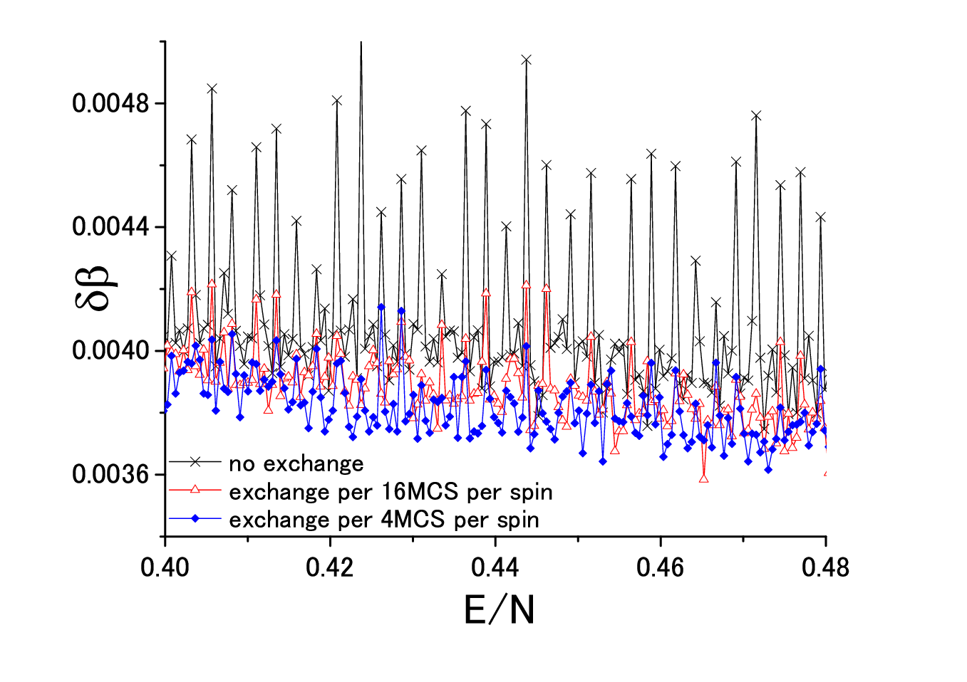
In order to check the efficiency of the replica exchange method, the sample to sample deviations of temperature, , where means average over samples, are shown in Fig. 3. The conditions of simulations are described in its caption. The peaks are observed in the system without exchange. The amplitudes of the peaks becomes smaller as the exchange frequency increases. The peaks exist at the seam points, which are the edges of the divided region. Except around the seam points, the reduction of fluctuations are moderate. This is because the present system does not exhibit large fluctuation for microcanonical state. The exchange method can work more effectively for the system with more complicated landscape in phase space.
IV Results
We perform simulation with and for system size by using threads. The density of states is calculated not for all energy region but restricted region of interest. The numerical data shown below are average over samples with different realizations of random number. In the Wang-Landau sampling we decrease the modification constant for step by step, (except for with and with , where modification constant is decreased down to ) with achieving 90 % flatness of energy histogram for all threads in every step. Typical number of total MCSs is per spin in the final step of simulations. The replica exchange is attempted in every 16 MCSs per spin.
IV.1 temperature vs internal energy characteristics
(a)

(b)

(a)

(b)

Figure 4 shows the inverse microcanonical temperature for and for various system size. While should be a monotonically decreasing function of to make the free energy a convex function of , it is not for the finite size system. In the region with positive derivative, i.e., negative specific heat, phase coexisting is observed as shown in Fig. 1. This state corresponds to the free energy maximum in the canonical ensemble. A dip and a peak exist inside the coexisting region in the thermodynamic limit, , where and for and and for . We note the bottom/top position of the dip/peak as = and , respectively. These points are regarded as the equilibrium spinodal points, i.e., saddle-node bifurcation points, where the second free energy minimum in canonical distribution annihilates together with one free energy maximum. As increasing system size, approaches and approaches for all with .
For , a plateau, where almost equals , is obviously observed in the middle of coexisting region. In this plateau region, the two coexisting phases form strips parallel to the horizontal or longitudinal axis, while minority phase forms a droplet in the side regions (see Fig. 1). With increasing system size, it is observed that the plateau region becomes wider and the step-like change of on the edge becomes sharper as a consequence of droplet-strip(slab) transition [10].
As increasing system size, the two spinodal points, , approach , respectively. The deviation and decreases as a power function of [20]. To show it clearly, we perform finite size scaling in Fig. 5 with expecting a formula
| (3) |
with a scaling function , that for isotherm lattice gas model is derived in Ref. [5], where and are replaced with magnetic field and magnetization, respectively. For , it is observed that the scaled curve approaches a large size limit; linearly increases as where is a specific heat, at in the evaporation phase and discontinuously drops down when entering the condensation phase. Note that this scaling does not aim the collapse of data to a universal curve as in standard finite size scaling for second order transitions, but it is intended to show the conversion to the large size limit by blowing up the transition region, which vanishes in macroscopic scale. (Scaling of finite size rounding may be a challenging problem.) On the other hand, discontinuous behavior is rarely observed in the system with even for . This is because correlation length is rather large and the used sample size is effectively much smaller than that for .
IV.2 volume fraction of a droplet

To observe the nature of droplet formation more directly, we estimate the ratio of condensation volume to the whole system volume. To this end, we divide a sample into square-shaped subsystems with size ( is approximated by the closest integer if necessary). This resolution is fine enough to capture the shape of the critical droplet with size of . We calculate energy per spin for each square, whose distribution function is shown in Fig. 6. Hereafter we only show the results for . Bimodal distribution is observed in the condensed regime, . The width of peaks becomes narrower as and the integral of bridge component between the two peaks corresponding to the perimeter of droplet becomes smaller with . The positions of the peaks hardly change with but only heights change for , which means that the change of state in this regime can be described only by the change of mixing ratio of the two phases. We determine a subsystem with energy below/above [16] belongs to the ferro/para domain.

The volume fraction of the para phase, , is plotted in Fig. 7. In the thermodynamic limit, equals zero for , unity for and linearly increases in between as . Finite size deviation is observed on the edge of the coexisting region as shown in the insets of Fig. 7. The fraction of condensed phase for finite size system is smaller than that for . The normalized condensation ratio
| (4) |
is expected to be a function of dimensionless variable,
| (5) | |||
| (6) |
for . Here is an interface free energy per volume of an optimally shaped large Wulff droplet [21]. The derivation of this formulae is described in Appendix A. The behavior in the thermodynamic limit is exactly known [4] as for and for . While is estimated as 5.41, is an only unknown quantity needed to calculate . By only assuming (then ), however, our numerical result shows good agreement with the theory as shown in Fig. 8. While decreases to zero for with increasing , very little finite size dependence is observed . The gap of at also coincides with the predicted value .

V Conclusion
We have investigated the condensation/evaporation transition of the Potts model in microcanonical ensemble. Interesting property of this transition is that it becomes impossible to be found in the true thermodynamic limit; the width of supersaturation regime disappears, but discontinuity of scaled quantities becomes clear with increasing system size. The present numerical results with show good agreement with the theoretical prediction of the system size dependence both for temperature [5] and condensation ratio [4]. Both of the two mean that droplet with size smaller than is unstable.
For finite size system in microcanonical ensemble, we observe negative (inverse) specific heat in the coexisting region and over/underhang of temperature, that corresponds to the thermodynamic spinodal point in canonical ensemble. The scaling behavior suggests an existence of a diverging length scale, . This means that a supersaturation state at given temperature becomes unstable at a length scale above . Although this length is related to the equilibrium spinodal point, it is not clear whether it also has some meanings in nonequilibrium dynamics, which may be an interesting open problem.
Last of all, let us note on the difficulty of the simulation of first order transitions. We suffered from slow relaxation for large system size in the present study as well as discussed in Ref. [10]. It is considered that the Wang-Landau sampling is quite efficient for first order transitions with discontinuity of as well as some other extended ensemble methods, such as the multicanonical method [22] because it provides additional probability weight on coexisting states to bridge the divide between two distinct homogeneous states, such as para and ferro phases. However there are still discontinuous transitions in the coexisting phase, that is a evaporation/condensation transition with discontinuity and droplet/slab transition, [10, 11]. This behavior is general for first order transitions. Since the problem is that the two states are energetically degenerate in these transitions, one fundamental solution to this problem may be to employ another argument which corresponds to the shape of domains for the joint density of state [18, 23]. Although it requires considerable amount of computation, massive parallel computation makes it feasible.
Appendix A finite size effect on droplet condensation ratio
Here we derive the condensation rate of a droplet for a energy driven phase transition by translating the result for a magnetization driven transition [4, 13]. We consider canonical ensemble at the bistable point and its energy distribution function around a peak at . (The case around the another peak is derived in the same way. )
We note the excess energy in fluctuation beyond the peak as and divide into two parts, , where is due to small bubble excitation and is due to a large droplet of disordered phase. If introducing condensation ratio as , the rest is given by . The volume of the droplet, , can be smaller than that in the thermodynamic limit, , for finite size system. By using these quantities, the energy distribution function is proportional to , where
| (7) | |||||
| (8) | |||||
| (9) |
The first term indicates the fluctuation without phase coexistence characterized by specific heat and the second term indicates the surface free energy of a large droplet.
The nature of the fluctuation depends on the dimensionless parameter which is related to the excess energy. For given , free energy is minimized at
| (10) |
which means supersaturation regime, while for minimum is given by a solution of
| (11) |
which means condensation regime. The two states with and is equivalently stable at .
This discontinuous change at is directly observed as a internal energy driven transition in microcanonical ensemble.
ACKNOWLEDGMENTS
This work was partly supported by Award No. KUK-I1-005-04 made by King Abdullah University of Science and Technology (KAUST).
References
- [1] P. A. Rikvold, H. Tomita, S. Miyashita, and S. W. Sides, Phys. Rev. E 49, 5080 (1994).
- [2] M. A. Novotny, G. Brown, and P. A. Rikvold, J. App. Phys. 91, 6908 (2002).
- [3] B. A. Berg and S. Dubey, Phys. Rev. Lett. 100, 165702 (2008).
- [4] M. Biskup, L. Chayes, and Kotecký, Europhys. Lett. 60, 21 (2002).
- [5] K. Binder, Physica A 319, 99 (2003).
- [6] K. Binder and M. H. Kalos, J. Stat. Phys. 22, 363 (1980).
- [7] L. G. MacDowell, P. Virnau, M. Müller, and K. Binder, J. Chem. Phys. 120, 5293 (2004).
- [8] L. G. MacDowell, V. K. Shen, and J. R. Errington, J. Chem. Phys. 125, 034705 (2006).
- [9] M. Schrader, P. Virnau, and K. Binder, Phys. Rev. E 79, 061104 (2009).
- [10] T. Neuhaus and J. S. Hager, J. Stat. Phys. 113, 1 (2003).
- [11] A. Nußbaumer, E. Bittner, T. Neuhaus, and W. Janke, Europhys. Lett. 75, 716 (2006).
- [12] S. S. Martinos, A. Malakis, and I. Hadjiagapiou, Physica A 384, 368 (2007).
- [13] A. Nußbaumer, E. Bittner, T. Neuhaus, and W. Janke, Prog. Theo. Phys. Suppl. 184, 400 (2010).
- [14] D. H. E. Gross, A. Ecker, and X. Z. Zhang, Ann. Physik 5, 446 (1996).
- [15] W. Janke, Nuc. Phys. B (Proc. Suppl.) 63A-C, 631 (1998).
- [16] F. Y. Wu, Rev. Mod. Phys. 54, 235 (1982).
- [17] F. Wang and D. P. Landau, Phys. Rev. Lett. 86, 2050 (2001).
- [18] D. P. Landau, S.-H. Tsai, and M. Exler, American J. Phys. 72, 1294 (2004).
- [19] K. Hukushima and K. Nemoto, J. Phys. Soc. Jpn. 65, 1604 (1996).
- [20] A. Bazavov, B. A. Berg, and S. Dubey, Nuc. Phys. B 802, 421 (2008).
- [21] G. Wulff, Z. Kristallogr. Mineral. 34, 449 (1901).
- [22] B. A. Berg and T. Neuhaus, Phys. Rev. Lett 68, 9 (1992).
- [23] C. Zhou, T. C. Schulthess, S. Torbrügge, and D. P. Landau, Phys. Rev. Lett. 96, 120201 (2006).